Using $k$-way Co-occurrences for Learning Word Embeddings

Abstract

Co-occurrences between two words provide useful insights into the semantics of those words. Consequently, numerous prior work on word embedding learning have used co-occurrences between two words as the training signal for learning word embeddings. However, in natural language texts it is common for multiple words to be related and co-occurring in the same context. We extend the notion of co-occurrences to cover $k(\geq\!\!2)$-way co-occurrences among a set of $k$-words. Specifically, we prove a theoretical relationship between the joint probability of $k(\geq\!\!2)$ words, and the sum of $\ell_{2}$ norms of their embeddings. Next, we propose a learning objective motivated by our theoretical result that utilises $k$-way co-occurrences for learning word embeddings. Our experimental results show that the derived theoretical relationship does indeed hold empirically, and despite data sparsity, for some smaller $k$ values, $k$-way embeddings perform comparably or better than $2$-way embeddings in a range of tasks.

1 Introduction

Word co-occurrence statistics are used extensively in a wide-range of NLP tasks for semantic modelling Turney and Pantel (2010); Church and Hanks (1990). As the popular quote from Firth—you shall know a word by the company it keeps Firth (1957), the words that co-occur with a particular word provide useful clues about the semantics of the latter word. Co-occurrences of a target word with other (context) words in some context such as a fixed-sized window, phrase, or a sentence have been used for creating word representations Mikolov et al. (2013b, a); Pennington et al. (2014). For example, skip-gram with negative sampling (SGNS) Mikolov et al. (2013a) considers the co-occurrences of two words within some local context, whereas global vector prediction (GloVe) Pennington et al. (2014) learns word embeddings that can predict the total number of co-occurrences in a corpus.

Unfortunately, much prior work in NLP are limited to the consideration of co-occurrences between two words due to the ease of modelling and data sparseness. Pairwise co-occurrences can be easily represented using a co-occurrence matrix, whereas co-occurrences involving more than two words would require a higher-order tensor Socher et al. (2013). Moreover, co-occurrences involving more than three words tend to be sparse even in large corpora Turney (2012), requiring compositional approaches for representing their semantics Zhang et al. (2014); Van de Cruys et al. (2013). It remains unknown – what statistical properties about words we can learn from $k$-way co-occurrences among words. Here, we use the term $k$-way co-occurrence to denote the co-occurrence between $k$-words in some context.

Words do not necessarily appear as pairs in sentences. By splitting the contexts into pairs of words, we loose the rich contextual information about the nature of the co-occurrences. For example, consider the following sentences.

1. John and Anne are friends.

2. John and David are friends.

3. Anne and Mary are friends.

Sentence (a) describes a three-way co-occurrence among (John, Anne, friend), which if split would result in three two-way co-occurrences: (John, Anne), (John, friends), and (Anne, friends). On the other hand, Sentences (b) and (c) would collectively produce the same two two-way co-occurrences (John, friend) and (Anne, friend), despite not mentioning any friendship between John and Anne. Therefore, by looking at the three two-way co-occurrences produced by Sentence (a) we cannot unambiguously determine whether John and Anne are friends. Therefore, we must retain the three-way co-occurrence (John, Anne, friend) to preserve this information.

Although considering $k$-way co-occurrences is useful for retaining the contextual information, there are several challenges one must overcome. First, the number of $k$-way co-occurrences tend to be sparse for larger $k$ values. Such sparse co-occurrence counts might be inadequate for learning reliable and accurate semantic representations. Second, the unique number of $k$-way co-occurrences grows exponentially with $k$. This becomes problematic in terms of memory requirements when storing all $k$-way co-occurrences. A word embedding learning method that considers $k$-way co-occurrences must overcome those two challenges.

In this paper, we make several contributions towards the understanding of $k$-way co-occurrences.

• We prove a theoretical relation between the joint probability of $k$ words, and the squared sum of $\ell_{2}$ norms of their embeddings (§3). For this purpose, we extend the work by Arora et al. (2016) for two-way co-occurrences to $k(>2)$-way co-occurrences.

• Motivated by our theoretical analysis, we propose an objective function that considers $k$-way co-occurrences for learning word embeddings (§4). We note that our goal in this paper is not to propose novel word embedding learning methods, nor we claim that $k$-way embeddings produce state-of-the-art results for word embedding learning. Nevertheless, we can use word embeddings learnt from $k$-way co-occurrences to empirically evaluate what type of information is captured by $k$-way co-occurrences.

• We evaluate the word embeddings created from $k$-way co-occurrences on multiple benchmark datasets for semantic similarity measurement, analogy detection, relation classification, and short-text classification (§5.2). Our experimental results show that, despite data sparsity, for smaller $k$-values such as 3 or 5, $k$-way embeddings outperform $2$-way embeddings.

2 Related Work

The use of word co-occurrences to learn lexical semantics has a long history in NLP Turney and Pantel (2010). Counting-based distributional models of semantics, for example, represent a target word by a high dimensional sparse vector in which the elements correspond to words that co-occur with the target word in some contextual window. Numerous word association measures such as pointwise mutual information (PMI) Church and Hanks (1990), log-likelihood ratio (LLR) Dunning (1993), $\chi^{2}$ measure Gale and Church (1991), etc. have been proposed to evaluate the strength of the co-occurrences between two words.

On the other hand, prediction-based approaches Mikolov et al. (2013a); Pennington et al. (2014); Collobert and Weston (2008); Mnih and Hinton (2009); Huang et al. (2012) learn low-dimensional dense embedding vectors that can be used to accurately predict the co-occurrences between words in some context. However, most prior work on co-occurrences have been limited to the consideration of two words, whereas continuous bag-of-words (CBOW) Mikolov et al. (2013a) model is a notable exception because it uses all the words in the context of a target word to predict the occurrence of the target word. The context can be modelled either as the concatenation or average of the context vectors. Models that preserve positional information in local contexts have also been proposed Ling et al. (2015).

Co-occurrences of multiple consecutive words in the form of lexico-syntactic patterns have been successfully applied in tasks that require modelling of semantic relations between two words. For example, Latent Relational Analysis (LRA) Turney (2006) represents the relations between word-pairs by a co-occurrence matrix where rows correspond to word-pairs and columns correspond to various lexical patterns that co-occur in some context with the word-pairs. The elements of this matrix are the co-occurrence counts between the word-pairs and lexical patterns. However, exact occurrences of $n$-grams tend to be sparse for large $n$ values, resulting in a sparse co-occurrence matrix Turney (2012). LRA uses singular value decomposition (SVD) to reduce the dimensionality, thereby reducing sparseness.

Despite the extensive applications of word co-occurrences in NLP, theoretical relationships between co-occurrence statistics and semantic representations have been less understood. Hashimoto et al. (2016) show that word embedding learning can be seen as a problem of metric recovery from log co-occurrences between words in a large corpus. Arora et al. (2016) show that log joint probability between two words is proportional to the squared sum of the $\ell_{2}$ norms of their embeddings. However, both those work are limited to two-way co-occurrences (i.e. $k=2$ case). In contrast, our work can be seen as extending this analysis to $k>2$ case. In particular, we show that under the same assumptions made by Arora et al. (2016), the log joint probability of a set of $k$ co-occurring words is proportional to the squared sum of $\ell_{2}$ norms of their embeddings.

Averaging word embeddings to represent sentences or phrases has found to be a simple yet an accurate method Arora et al. (2017); Kenter et al. (2016) that has reported comparable performances to more complex models that consider the ordering of words Kiros et al. (2015). For example, Arora et al. (2017) compute sentence embeddings as the linearly weighted sum of the constituent word embeddings, where the weights are computed using unigram probabilities, whereas Rei and Cummins (2016) propose a task-specific supervised approach for learning the combination weights. Kenter et al. (2016) learn word embeddings such that when averaged produce accurate sentence embeddings. Such prior work hint at the existence of a relationship between the summation of the word embeddings, and the semantics of the sentence that contains those words. However, to the best of our knowledge, a theoretical connection between $k$-way co-occurrences and word embeddings has not been established before.

3 $k$-way word co-occurrences

Our analysis is based on the random walk model of text generation proposed by Arora et al. (2016) Let $\mathcal{V}$ be the vocabulary of words. Then, the $t$-th word $w_{t}\in\mathcal{V}$ is produced at step $t$ by a random walk driven by a discourse vector $\bm{c}_{t}\in\mathbb{R}^{d}$. Here, $d$ is the dimensionality of the embedding space and coordinates of $\bm{c}_{t}$ represent what is being talked about. Moreover, each word $w\in\mathcal{V}$ is represented by a vector (embedding) $\bm{w}\in\mathbb{R}^{d}$. Under this model, the probability of emitting $w\in\mathcal{V}$ at time $t$, given $\bm{c}_{t}$ given by (1).

$$\textrm{Pr}[\text{emitting $w$ at time $t$}\mid\bm{c}_{t}]\propto\exp\left(\bm{c}_{t}{}^{\top}\bm{w}\right)$$ (1)

Here, a slow random work is assumed where $\bm{c}_{t+1}$ can be obtained from $\bm{c}_{t}$ by adding a small random displacement vector such that nearby words are generated under similar discourses. More specificaly, we assume that $\textrm{~{}}\arrowvert\textrm{~{}}\bm{c}_{t+1}-\bm{c}_{t}\textrm{~{}}\arrowvert\textrm{~{}}_{2}\leq\epsilon_{2}/\sqrt{d}$ for some small $\epsilon_{2}>0$. The stationary distribution $\mathcal{C}$ of the random walk is assumed to be uniform over the unit sphere. For such a random walk, Arora et al. (2016) prove the following Lemma.

Lemma 1 (Concentration of Partition functions Lemma 2.1 of Arora et al. (2016)).

If the word embedding vectors satisfy the Bayesian prior $\bm{v}=s\hat{\bm{v}}$, where $\bm{\hat{v}}$ is from the spherical Gaussian distribution, and $s$ is a scalar random variable, which is always bounded by a constant, then the entire ensemble of word vectors satisfies that

$$\Pr_{c\sim\mathcal{C}}[(1-\epsilon_{z})Z\leq Z_{c}\leq(1+\epsilon_{z})Z]\geq 1-\delta,$$ (2)

for $\epsilon_{z}=O(1/\sqrt{n})$, and $\delta=\exp(-\Omega(\log^{2}n))$, where $n\geq d$ is the number of words and $Z_{c}$ is the partition function for $c$ given by $\sum_{w\in\mathcal{V}}\exp\left(\bm{w}{}^{\top}\bm{c}\right)$.

Lemma 1 states that the partition function concentrates around a constant value $Z$ for all $c$ with high probability.

For $d$ dimensional word embeddings, the relationship between the $\ell_{2}$ norm of word embeddings $\bm{w}_{i}$, $\left|\left|\bm{w}_{i}\right|\right|_{2}$, and the joint probability of the words, $p(w_{1},\ldots,w_{k})$ is given by the following theorem:

Theorem 1.

Suppose the word vectors satisfy (2). Then, we have

$$\log p(w_{1},\ldots,w_{k})=\frac{\left|\left|\sum_{i=1}^{k}\bm{w}_{i}\right|\right|_{2}^{2}}{2d}-k\log Z\pm\epsilon.$$ (3)

for $\epsilon=O(k\epsilon_{z})+\widetilde{O}(1/d)+O(k^{2}\epsilon_{2})$, where

$$\small Z=\sum_{(w_{1},\ldots,w_{k})\in\mathcal{V}^{k}}\sum_{c\in\mathcal{C}}\exp\left(\sum_{i=1}^{k}\bm{w}_{i}^{\top}\bm{c}\right).$$ (4)

Note that the normalising constant (partitioning function) $Z$ given by (4) is independent of the co-occurrences.

Proof of Theorem 1 is given in the Appendix. In particular, for $k=1$ and $2$, Theorem 1 reduces to the relationships proved by Arora et al. (2016). Typically the $\ell_{2}$ norm of $d$ dimensional word vectors is in the order of $\sqrt{d}$, implying that the order of the squared $\ell_{2}$ norm of $\sum_{i=1}^{k}\bm{w}_{i}$ is $\mathcal{O}(d)$. Consequently, the noise level $\mathcal{O}(\epsilon)$ is significantly smaller compared to the first term in the left hand side. Later in § 5.1, we empirically verify the relationship stated in Theorem 1 and the concentration properties of the partitioning function for $k$-way co-occurrences.

4 Learning $k$-way Word Embeddings

In this Section, we propose a training objective that considers $k$-way co-occurrences using the relationship given by Theorem 1. By minimising the proposed objective we can obtain word embeddings that consider $k$-way co-occurrences among words. The word embeddings derived in this manner serve as a litmus test for empirically evaluating the validity of Theorem 1.

Let us denote the $k$-way co-occurrence $(w_{1},\ldots,w_{k})=w_{1}^{k}$, and its frequency in a corpus by $h(w_{1}^{k})$. The joint probability $p(w_{1}^{k})$ of such a $k$-way co-occurrence is given by (3). Although successive samples from a random walk are not independent, if we assume the random walk to mix fairly quickly (i.e. mixing time related to the logarithm of the vocabulary size), then the distribution of $h(w_{1}^{k})$ can be approximated by a multinomial distribution $\textsf{Mul}\left(\tilde{L}_{k},\{p(w_{1}^{k})\}\right)$, where $\tilde{L}_{k}=\sum_{w_{1}^{k}\in\mathcal{G}_{k}}h(w_{1}^{k})$ and $\mathcal{G}_{k}$ is the set of all $k$-way co-occurrences. Under this approximation, Theorem 2 provides an objective for learning word embeddings from $k$-way co-occurrences.

Theorem 2.

The set of word embeddings $\{\bm{w}_{i}\}$ that minimise the objective given by (5) maximises the log-likelihood of $k$-way co-occurrences given by (6). Here, $C$ is a constant independent of the word embeddings.

$$\sum_{w_{1}^{k}\in\mathcal{G}_{k}}h(w_{1}^{k})\left(\log(h(w_{1}^{k}))-\left|\left|\sum_{i=1}^{k}\bm{w}_{i}\right|\right|_{2}^{2}+C\right)^{2}$$ (5)

$$l=\log\left(\prod_{w_{1}^{k}\in\mathcal{G}_{k}}{p(w_{1}^{k})}^{h(w_{1}^{k})}\right)$$ (6)

Proof.

The log-likelihood term can we written as

$$l=\sum_{w_{1}^{k}\in\mathcal{G}_{k}}h(w_{1}^{k})\log p(w_{1}^{k}).$$ (7)

The expected count of a $k$-way co-occurrence $w_{1}^{k}$ can be estimated as $\tilde{L}_{k}p(w_{1}^{k})$. We then define the log-ratio between the expected and actual $k$-way co-occurrence counts $\Delta_{w_{1}^{k}}$ as

$$\Delta_{w_{1}^{k}}=\log\left(\frac{\tilde{L}_{k}p(w_{1}^{k})}{h(w_{1}^{k})}\right).$$ (8)

Substituting for $p(w_{1}^{k})$ from (8) in (7) we obtain

$$l=\sum_{w_{1}^{k}\in\mathcal{G}_{k}}h(w_{1}^{k})\left(\Delta_{w_{1}^{k}}-\log\tilde{L}_{k}+\log h(w_{1}^{k})\right).$$ (9)

Representing the terms independent from the embeddings $\bm{w}_{k}$ by $C$ we can re-write (9) as

$$l=C+\sum_{w_{1}^{k}\in\mathcal{G}_{k}}h(w_{1}^{k})\Delta_{w_{1}^{k}}.$$ (10)

Because $p(w_{1}^{k})$ represents a joint probability distribution over $k$-way co-occurrences $w_{1}^{k}$ we have

$$\tilde{L}_{k}=\sum_{w_{1}^{k}\in\mathcal{G}_{k}}\tilde{L}_{k}p(w_{1}^{k}).$$ (11)

Substituting (8) in (11) we obtain

$$\tilde{L}_{k}=\sum_{w_{1}^{k}\in\mathcal{G}_{k}}h(w_{1}^{k})\exp\left(\Delta_{w_{1}^{k}}\right).$$ (12)

When $x$ is small, from Taylor expansion $\exp(x)\approx 1+x+x^{2}/2$ we have

$$\tilde{L}_{k}\approx\sum_{w_{1}^{k}\in\mathcal{G}_{k}}h(w_{1}^{k})\left(1+\Delta_{w_{1}^{k}}+\frac{\Delta^{2}_{w_{1}^{k}}}{2}\right)$$ (13)

Although this Taylor expansion has an approximation error of $\mathcal{O}(x^{3})$, for large $h(w_{1}^{k})$ values, expected counts approach actual counts resulting in $\Delta_{k}$ values closer to 0 according to (8). On the other hand, word co-occurrence counts approximately follow a power-law distribution Pennington et al. (2014). Therefore, contributions to the objective function by $\Delta_{w_{1}^{k}}$ terms corresponding to smaller $h(w_{1}^{k})$ can be ignored in practice. Then, by definition we have

$$\tilde{L}_{k}=\sum_{w_{1}^{k}\in\mathcal{G}_{k}}h(w_{1}^{k}).$$ (14)

By substituting (14) in (13) we obtain

$$\sum_{w_{1}^{k}\in\mathcal{G}_{k}}h(w_{1}^{k})\Delta_{w_{1}^{k}}\approx-\frac{1}{2}\sum_{w_{1}^{k}\in\mathcal{G}_{k}}h(w_{1}^{k})\Delta^{2}_{w_{1}^{k}}.$$ (15)

From (10) and (15) we obtain

$$l=C-\frac{1}{2}\sum_{w_{1}^{k}\in\mathcal{G}_{k}}h(w_{1}^{k})\Delta^{2}_{w_{1}^{k}}.$$ (16)

Therefore, minimisation of $\sum_{w_{1}^{k}\in\mathcal{G}_{k}}h(w_{1}^{k})\Delta^{2}_{w_{1}^{k}}$ corresponds to the maximisation of the log-likelihood. ∎

Minimising the objective (5) with respect to $\bm{w}_{i}$ and $C$ produces word embeddings that capture the relationships in $k$-way co-occurrences of words in a corpus. Down-weighting very frequent co-occurrences of words has shown to be effective in prior work. This can be easily incorporated into the objective function (5) by replacing $h(w_{1}^{k})$ by a truncated version such as $\min(h(w_{1}^{k}),\theta_{k})$, where $\theta$ is a cut-off threshold, where we set $\theta=100$ following prior work. We find the word embeddings $\bm{w}_{i}$ for a set of $k$-way co-occurrences $\mathcal{G}_{k}$ and the parameter $C_{k}$, by computing the partial derivative of the objective given by Equation 5 w.r.t. those parameters, and applying Stochastic Gradient Descent (SGD) with learning rate updated using AdaGrad Duchi et al. (2011). The initial learning rate is set to $0.01$ in all experiments. We refer to the word embeddings learnt by optimising (5) as $k$-way embeddings.

5 Experiments

We pre-processed a January 2017 dump of English Wikipedia using a Perl script and used as our corpus (contains ca. 4.6B tokens). We select unigrams occurring at least $1000$ times in this corpus amounting to a vocabulary of size $73,954$. Although it is possible to apply the concept of $k$-way co-occurrences to $n$-grams of any length $n$, for the simplicity we limit the analysis to co-occurrences among unigrams. Extracting $k$-way co-occurrences from a large corpus is challenging because of the large number of unique and sparse $k$-way co-occurrences. Note that $k$-way co-occurrences are however less sparse and less diverse compared to $k$-grams because the ordering of words is ignored in a $k$-way co-occurrence. Following the Apriori algorithm Agrawal and Srikant (1994) for extracting frequent itemsets of a particular length with a pre-defined support, we extract $k$-way co-occurrences that occur at least $1000$ times in the corpus within a $10$ word window.

Specifically, we select all $(k-1)$-way co-occurrences that occur at least $1000$ times and grow them by appending the selected unigrams (also occurring at least $1000$ times in the corpus). We then check whether all subsets of length $(k-1)$ of a candidate $k$-way co-occurrence appear in the set of frequent $(k-1)$-way co-occurrences. If this requirement is satisfied, then it follows from the apriori property that the generated $k$-way co-occurrence must have a minimum support of $1000$. Following this procedure we extract $k$-way co-occurrences for $k=2,3,4$, and $5$ as shown in Table 1.

$k$	no. of $k$-way co-occurrences
2	257,508,996
3	394,670,208
4	111,119,411
5	14,495,659

Table 1: The number of unique $k$-way co-occurrence with support $1000$.

5.1 Empirical Verification of the Model

(a) 2-way co-occurrences

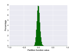
(b) 3-way co-occurrences

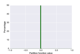
(c) 4-way co-occurrences

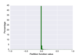
(d) 5-way co-occurrences

Figure 1: Histogram of the partitioning function for randomly chosen $10,000$ context vectors.

Our proof of Theorem 1 requires the condition used in Lemma 1, which states that the partition function given by (4) must concentrate within a small range for any $k$. Although such concentration properties for $2$-way co-occurrences have been reported before, it remains unknown whether this property holds for $k(>\!\!2)$-way co-occurrences. To test this property empirically, we uniformly randomly generate $10^{5}$ vectors $\bm{c}$ ($\ell_{2}$ normalised to unit length) and compute the histogram of the partition function values as shown in Figure 1 for $d=300$ dimensional embeddings. We standardise the histogram to zero mean and unit variance for the ease of comparisons. From Figure 1, we see that the partition function concentrates around the mean for all $k$-values. Interestingly, the concentration is stronger for higher $k(>\!\!3$) values. Because we compute the sum of the embeddings of individual words in (4), from the law of large numbers it follows that the summation converges towards the mean when we have more terms in the $k$-way co-occurrence. This result shows that the assumption on which Theorem 1 is based (i.e. concentration of the partition function for arbitrary $k$-way co-occurrences), is empirically justified.

Next, to empirically verify the correctness of Theorem 1, we learn $d=300$ dimensional $k$-way embeddings for each $k$ value in range $[2,5]$ separately , and measure the Spearman correlation between $\log p(w_{1},\ldots,w_{k})$ and $\left|\left|\sum_{i=1}^{k}\bm{w}_{i}\right|\right|_{2}^{2}$ for a randomly selected $10^{6}$ $k$-way co-occurrences. If (3) is correct, then we would expect a linear relationship (demonstrated by a high positive correlation) between the two sets of values for a fixed $k$.

Figure 2 shows the correlation plots for $k=2,3,4$, and $5$. From Figure 2 we see that there exist such a positive correlation in all four cases. However, the value of the correlation drops when we increase $k$ as a result of the sparseness of $k$-way co-occurrences for larger $k$ values. Although due to the limited availability of space we show results only for $d=300$ embeddings, the above-mentioned trends could be observed across a wide range of dimensionalities ($d\in[50,1000]$) in our experiments.

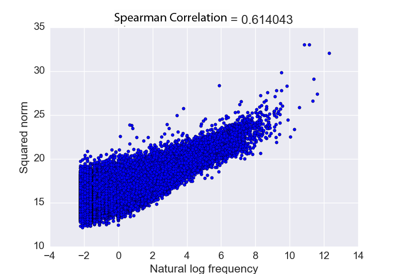
(a) 2-way co-occurrences

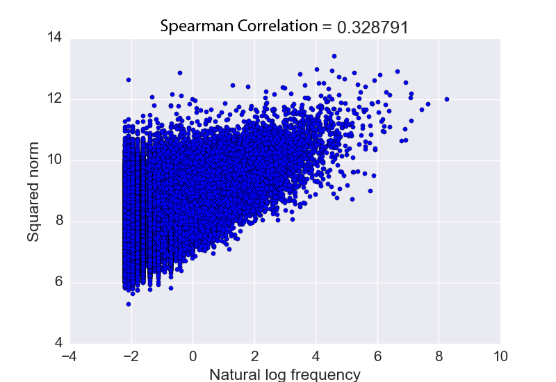
(b) 3-way co-occurrences

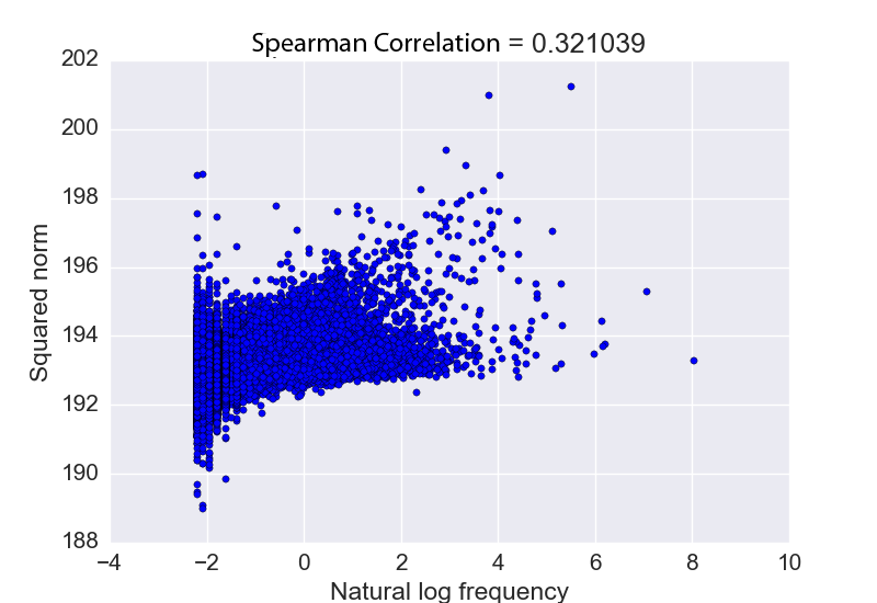
(c) 4-way co-occurrences

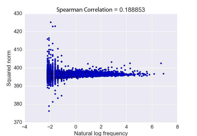
(d) 5-way co-occurrences

Figure 2: Correlation between the squared $\ell_{2}$ norms of the sum of the $k$-way embeddings and the natural log frequency of the corresponding $k$-way co-occurrences are shown for different $k$ values.

5.2 Evaluation of Word Embeddings

$k$	RG	MC	WS	RW	SCWS	MEN	SL	SE	DV	TR	MR	CR	SUBJ
$2$	78.63	79.17	59.68	41.53	57.09	70.42	34.76	37.21	75.34	72.43	68.38	79.19	82.20
$\leq 3$	77.51	79.92	59.61	41.58	56.69	$\mathbf{70.92}^{*}$	34.65	37.42	$\mathbf{75.96}^{*}$	$\mathbf{72.92}^{*}$	68.71	$\mathbf{79.52}^{*}$	82.35
$\leq 4$	75.85	72.66	59.75	41.23	56.74	70.32	34.51	37.01	74.92	72.37	67.87	78.18	82.25
$\leq 5$	75.19	74.63	$\mathbf{60.54}^{*}$	40.84	56.92	70.50	34.67	37.21	74.76	72.21	68.48	77.18	$\mathbf{82.60}^{*}$

Table 2: The results on word similarity, analogy, relation classification and short-text classification tasks reported by the word embeddings learnt using $k$-way co-occurrences for different $k$ values.

We re-emphasise here that our goal in this paper is not to propose novel word embedding learning methods but to extend the notion of $2$-way co-occurrences to $k$-way co-occurrences. Unfortunately all existing word embedding learning methods use only $2$-way co-occurrence information for learning. Moreover, direct comparisons against different word embedding learning methods that use only $2$-way co-occurrences are meaningless here because the performances of those pre-trained embeddings will depend on numerous factors such as the training corpora, co-occurrence window size, word association measures, objective function being optimised, and the optimisation methods. Nevertheless, by evaluating the $k$-way embeddings learnt for different $k$ values using the same resources, we can empirically evaluate the amount of information captured by $k$-way co-occurrences.

For this purpose, we use four tasks that have been used previously for evaluating word embeddings.

Semantic similarity measurement:

We measure the similarity between two words as the cosine similarity between the corresponding embeddings, and measure the Spearman correlation coefficient against the human similarity ratings. We use Rubenstein and Goodenough (1965) (RG, 65 word-pairs), Miller and Charles (1998) (MC, 30 word-pairs), rare words dataset (RW, 2034 word-pairs) Luong et al. (2013), Stanford’s contextual word similarities (SCWS, 2023 word-pairs) Huang et al. (2012), the MEN dataset (3000 word-pairs) Bruni et al. (2012), and the SimLex SL dataset Hill et al. (2015) (999 word-pairs).

Word analogy detection:

Using the CosAdd method, we solve word-analogy questions in the SemEval (SE) dataset Jurgens et al. (2012). Specifically, for three given words $a$, $b$ and $c$, we find a fourth word $d$ that correctly answers the question $a$ to $b$ is $c$ to what? such that the cosine similarity between the two vectors $(\bm{b}-\bm{a}+\bm{c})$ and $\bm{d}$ is maximised.

Relation classification:

We use the DiffVec DV Vylomova et al. (2016) dataset containing 12,458 triples of the form $(\textrm{relation},\textrm{word}_{1},\textrm{word}_{2})$ covering 15 relation types. We train a 1-nearest neighbour classifier, where for each target tuple we measure the cosine similarity between the vector offset for its two word embeddings, and those of the remaining tuples in the dataset. If the top ranked tuple has the same relation as the target tuple, then it is considered to be a correct match. We compute the (micro-averaged) classification accuracy over the entire dataset as the evaluation measure.

Short-text classification:

We use four binary short-text classification datasets: Stanford sentiment treebank (TR) (903 positive test instances and 903 negative test instances), movie reviews dataset (MR) Pang and Lee (2005) (5331 positive instances and 5331 negative instances), customer reviews dataset (CR) Hu and Liu (2004) (925 positive instances and 569 negative instances), and the subjectivity dataset (SUBJ) Pang and Lee (2004) (5000 positive instances and 5000 negative instances). Each review is represented as a bag-of-words and we compute the centroid of the embeddings for each bag to represent the review. Next, we train a binary logistic regression classifier using the train portion of each dataset, and evaluate the classification accuracy using the corresponding test portion.

Statistical significance at $p<0.05$ level is evaluated for correlation coefficients and classification accuracies using respectively Fisher transformation and Clopper-Pearson confidence intervals.

Learning $k$-way embeddings from $k$-way co-occurrences for a single $k$ value results in poor performance because of data sparseness. To overcome this issue we use all co-occurrences equal or below a given $k$ value when computing $k$-way embeddings for a given $k$. Training is done in an iterative manner where we randomly initialise word embeddings when training $k=2$-way embeddings, and subsequently use $(k-1)$-way embeddings as the initial values for training $k$-way embeddings. The performances reported by $300$ dimensional embeddings are shown in Table 2, where best performance in each task is shown in bold and statistical significance over $2$-way embeddings is indicated by an asterisk.

From Table 2, we see that for most of the tasks the best performance is reported by $k(\geq 2)$-way embeddings and not $k=2$-way embeddings. In some of the larger datasets, the performances reported by $k\leq 3$ (for MEN, DV, and CR) and $k\leq 5$ way embeddings (for WS and SUBJ) are significantly better than that by the $2$-way embeddings. This result supports our claim that $k(>2)$-way co-occurrences should be used in addition to $2$-way co-occurrences when learning word embeddings.

Prior work on relational similarity measurement have shown that the co-occurrence context between two words provide useful clues regarding the semantic relations that exist between those words. For example, the the phrase is a large in the context Ostrich is a large bird indicates a hypernymic relation between ostrich and bird. The two datasets SE and DV evaluate word embeddings for their ability to represent semantic relations between two words. Interestingly, we see that $k\leq 3$ embeddings perform best on those two datasets.

Text classification tasks require us to understand not only the meaning of individual words but also the overall topic in the text. For example, in a product review individual words might have both positive and negative sentiments but for different aspects of the product. Consequently, we see that $k\leq 3$ embeddings consistently outperform $k=2$ embeddings on all short-text classification tasks. By consider all co-occurrences for $k\leq 5$ we see that we obtain the best performance on the SUBJ dataset.

For the word similarity benchmarks, which evaluate the similarity between two words, we see that $2$-way co-occurrences are sufficient to obtain the best results in most cases. A notable exception is WS dataset, which has a high portion of related words than datasets such as MEN or SL. Because related words can co-occur in broader contextual window and with various words, considering a $k\leq 5$ way co-occurrences seem to be effective.

5.3 Qualitative Evaluation

Our quantitative experiments revealed that 3-way embeddings are particularly better than 2-way embeddings in multiple tasks. To qualitatively evaluate the difference between 2-way and 3-way embeddings, we conduct the following experiment.

First, we combine all word pairs in semantic similarity benchmarks to create a dataset containing 8483 word pairs with human similarity ratings. We normalise the human similarity ratings in each dataset separately to $[0,1]$ range by subtracting the minimum rating and dividing by the difference between maximum and minimum ratings. The purpose of this normalisation is to make the ratings in different benchmark datasets comparable. Next, we compute the cosine similarity between the two words in each word pair using 2-way and 3-way embeddings separately. We then select word pairs where the difference between the two predicted similarity scores are significantly greater than one standard deviation point. This process yields $911$ word pairs, which we manually inspect and classify into several categories.

LABEL:tbl:qual shows some randomly selected word pairs with their predicted similarity scores scaled to 0.5 means and 1.0 variance, and human ratings given in the original benchmark dataset in which the word pair appears. We found that 2-way embeddings assign high similarity scores for many unrelated word pairs, whereas by using 3-way embeddings we are able to reduce the similarity scores assigned to such unrelated word pairs. Words such as giraffe, car and happy are highly frequent and co-occur with many different words. Under 2-way embeddings, any word that co-occur with a target word will provide a semantic attribute to the target word. Therefore, unrelated word pairs where at least one word is frequent are likely to obtain relatively higher similarity score under 2-way embeddings.

We see that the similarity between two words in a collocation are overly estimated by 2-way embeddings. The two words forming a collocation are not necessarily semantically similar. For example, movie and star do not share many attributes in common. 3-way embeddings correctly assigns lower similarity scores for such words because many other words co-occur with a particular collocation in different contexts.

We observed that 2-way embeddings assign high similarity scores for a large number of antonym pairs. Prior work on distributional methods of word representations have shown that it is difficult to discriminate between antonyms and synonyms using their word distributions (Mohammad:CL:2013). scheible-schulteimwalde-springorum:2013:IJCNLP show that by restricting the contexts we use for building such distributional models, by carefully selecting context features such as by selecting verbs it is possible to overcome this problem to an extent. Recall that 3-way co-occurrences require a third word co-occurring in the contexts that contain the co-occurrence between two words we are interested in measuring similarity. Therefore, 3-way embeddings by definition impose contextual restrictions that seem to be a promising alternative for pre-selecting contextual features. We plan to explore the possibility of using 3-way embeddings for discriminating antonyms in our future work.

6 Conclusion

We proved a theoretical relationship between joint probability of more than two words and their embeddings. Next, we learnt word embeddings using $k$-way co-occurrences to understand the types of information captured in a $k$-way co-occurrence. Our experimental results empirically validated the derived relationship. Moreover, by considering $k$-way co-occurrences beyond $2$-way co-occurrences, we can learn better word embeddings for tasks that require contextual information such as analogy detection and short-text classification.

Appendix

In this supplementary, we prove the main theorem (Theorem 1) stated in the paper. The definitions of the symbols and notation are given in the paper.

Theorem 3.

Suppose the word vectors satisfy (2) in the paper. Then, we have

$$\log p(w_{1},\ldots,w_{k})=\frac{\left|\left|\sum_{i\in[k]}\bm{w}_{i}\right|\right|_{2}^{2}}{2d}-k\log Z\pm\epsilon.$$

for $\epsilon=O(k\epsilon_{z})+\widetilde{O}(1/d)+O(k^{2}\epsilon_{2})$.

Proof.

Let $c_{i}\textrm{~{}}{\bm{;}}\textrm{~{}}(i\in\{1,\ldots,k\})$ be the hidden discourse that determines the probability of word $w_{i}$. We use $p(c_{i+1}\mid c_{i})\textrm{~{}}{\bm{;}}\textrm{~{}}(i\in\{1,\ldots,k-1\})$ to denote the Markov kernel (transition matrix) of the Markov chain. Let $\mathcal{C}$ be the stationary distribution of discourse $c$, and $\mathcal{D}$ be the joint distribution of $c_{[k]}=(c_{1},\ldots,c_{k})$. We marginalise over the contexts $c_{1},\ldots,c_{k}$ and then use the independence of $w_{1},\ldots,w_{k}$ conditioned on $c_{1},\ldots,c_{k}$,

$$p(w_{1},\ldots,w_{k})=\mathbb{E}_{c_{[k]}\sim\mathcal{D}}\Bigl{[}\prod_{i\in[k]}\frac{\exp(\langle\bm{w}_{i},\bm{c}_{i}\rangle)}{Z_{c_{i}}}\Bigr{]}.$$ (17)

We first get rid of the partition function $Z_{c_{i}}$ using Lemma 1 stated in the paper. Let $\mathcal{F}_{i}$ be the event that $c_{i}$ satisfies

$$(1-\epsilon_{z})Z\leq Z_{c_{i}}\leq(1+\epsilon_{z})Z.$$

Let $\mathcal{F}=\bigcap_{i\in[k]}\mathcal{F}_{i}$, and $\overline{\mathcal{F}}$ be its negation. Moreover, let ${\bm{1}}_{\mathcal{F}}$ be the indicator function for the event $\mathcal{F}$. By Lemma 1 and the union bound, we have $\mathbb{E}[{\bm{1}}_{\mathcal{F}}]=\Pr[\mathcal{F}]\geq 1-k\exp(-\Omega(\log^{2}n))$.

We first decompose (17) into the two parts according to whether event $\mathcal{F}$ happens, that is,

$$p(w_{1},\ldots,w_{k})=\mathbb{E}_{c_{[k]}\sim\mathcal{D}}\Bigl{[}\prod_{i\in[k]}\frac{\exp(\langle\bm{w}_{i},\bm{c}_{i}\rangle)}{Z_{c_{i}}}{\bm{1}}_{\mathcal{F}}\Bigr{]}+\mathbb{E}_{c_{[k]}\sim\mathcal{D}}\Bigl{[}\prod_{i\in[k]}\frac{\exp(\langle\bm{w}_{i},\bm{c}_{i}\rangle)}{Z_{c_{i}}}{\bm{1}}_{\overline{\mathcal{F}}}\Bigr{]}$$ (18)

We bound the first quantity using (1) in the paper and the definition of $\mathcal{F}$. That is,

$$\mathbb{E}_{c_{[k]}\sim\mathcal{D}}\Bigl{[}\prod_{i\in[k]}\frac{\exp(\langle\bm{w}_{i},\bm{c}_{i}\rangle)}{Z_{c_{i}}}{\bm{1}}_{\mathcal{F}}\Bigr{]}\leq\frac{(1+\epsilon_{z})^{k}}{Z^{k}}\mathbb{E}_{c_{[k]}\sim\mathcal{D}}\Bigl{[}\prod_{i\in[k]}\exp(\langle\bm{w}_{i},\bm{c}_{i}\rangle){\bm{1}}_{\mathcal{F}}\Bigr{]}.$$ (19)

For the second quantity, we have by Cauchy-Schwartz,

$$\left(\mathbb{E}_{c_{[k]}\sim\mathcal{D}}\Bigl{[}\prod_{i\in[k]}\frac{\exp(\langle\bm{w}_{i},\bm{c}_{i}\rangle)}{Z_{c_{i}}}{\bm{1}}_{\overline{\mathcal{F}}}\Bigr{]}\right)^{2} \leq\prod_{i\in[k]}\left(\mathbb{E}_{c_{[k]}\sim\mathcal{D}}\Bigl{[}\frac{\exp(\langle\bm{w}_{i},\bm{c}_{i}\rangle)^{2}}{Z_{c_{i}}^{2}}{\bm{1}}_{\overline{\mathcal{F}}}\Bigr{]}\right)$$

$$\leq\prod_{i\in[k]}\left(\mathbb{E}_{c_{i}}\Bigl{[}\frac{\exp(\langle\bm{w}_{i},\bm{c}_{i}\rangle)^{2}}{Z_{c_{i}}^{2}}\mathbb{E}_{c_{-i}\mid c_{i}}{\bm{1}}_{\overline{\mathcal{F}}}\Bigr{]}\right),$$ (20)

where $c_{-i}$ denotes the tuple obtained by removing $c_{i}$ from the tuple $(c_{1},\ldots,c_{k})$.

Using the argument as in Arora et al. (2016), we can show that

$$\mathbb{E}_{c_{i}}\Bigl{[}\frac{\exp(\langle\bm{w}_{i},\bm{c}_{i}\rangle)^{2}}{Z_{c_{i}}^{2}}\mathbb{E}_{c_{-i}\mid c_{i}}{\bm{1}}_{\overline{\mathcal{F}}}\Bigr{]}\leq k\exp(-\Omega(\log^{1.8}n)).$$

Hence by (20), the second quantity is bounded by $k^{k}\exp(-\Omega(k\log^{1.8}n))$. Combining this with (18) and (19), we obtain

$$p(w_{1},\ldots,w_{k}) \leq\frac{(1+\epsilon_{z})^{k}}{Z^{k}}\mathbb{E}_{c_{[k]}\sim\mathcal{D}}\Bigl{[}\prod_{i\in[k]}\exp(\langle\bm{w}_{i},\bm{c}_{i}\rangle){\bm{1}}_{\mathcal{F}}\Bigr{]}+k^{k}\exp(-\Omega(k\log^{1.8}n))$$

$$\leq\frac{(1+\epsilon_{z})^{k}}{Z^{k}}\mathbb{E}_{c_{[k]}\sim\mathcal{D}}\Bigl{[}\prod_{i\in[k]}\exp(\langle\bm{w}_{i},\bm{c}_{i}\rangle)\Bigr{]}+\delta_{0}$$

where

$$\delta_{0}=k^{k}\exp(-\Omega(k\log^{1.8}n))Z^{k}\leq k^{k}\exp(-\Omega(k\log^{1.8}n)).$$

The last inequality is due to the fact that $Z\leq\exp(2\kappa)n=O(n)$, where $\kappa$ is the upper bound on $s$ used to generate word embedding vectors, which is regarded as a constant.

On the other hand, we can lowerbound similarly

$$p(w_{1},\ldots,w_{k})\geq\frac{(1-\epsilon_{z})^{k}}{Z^{k}}\mathbb{E}_{c_{[k]}\sim\mathcal{D}}\Bigl{[}\prod_{i\in[k]}\exp(\langle\bm{w}_{i},\bm{c}_{i}\rangle)\Bigr{]}-\delta_{0}$$

Taking logarithm, the multiplicative error translates to an additive error

$$\log p(w_{1},\ldots,w_{k})= \log\left(\mathbb{E}_{c_{[k]}\sim\mathcal{D}}\left[\prod_{i\in[k]}\exp(\langle\bm{w}_{i},\bm{c}_{i}\rangle)\right]\pm\delta_{0}\right)-k\log Z+k\log(1\pm\epsilon_{z}).$$

For the purpose of exploiting the fact that $c_{1},\ldots,c_{k}$ should be close to each other, we further rewrite $\log p(w_{1},\ldots,w_{k})$ by re-organizing the expectations above,

$$\log p(w_{1},\ldots,w_{k})=\log\Bigl{(}A_{1}\pm\delta_{0}\Bigr{)}-k\log Z+k\log(1\pm\epsilon_{z}).$$ (21)

where $A_{1},\ldots,A_{k}$ are defined as

$$A_{i} =\mathbb{E}_{c_{i}\mid c_{1},\ldots,c_{i-1}}\Bigl{[}\exp(\langle\bm{w}_{i},\bm{c}_{i}\rangle)A_{i+1}\Bigr{]}\quad i\in[k],$$

$$A_{k+1} =1.$$

Here, we regard $c_{0}$ is a discourse uniformly sampled from $\mathcal{C}$. Then, we inductively show that

$$A_{i}=(1\pm\epsilon_{2})^{k(k-i+1)}\exp\left(\langle\sum_{j=i}^{k}\bm{w}_{j},\bm{c}_{i-1}\rangle\right).$$

The base case $i=k+1$ clearly holds.

Suppose that the claim holds for $i+1$. Since $\left|\left|\bm{w}_{j}\right|\right|\leq\kappa\sqrt{d}$ for every $j\in\{i,\ldots,k\}$, we have that

$$\langle\sum_{j=i}^{k}\bm{w}_{j},\bm{c}_{i-1}-\bm{c}_{i}\rangle\leq\left|\left|\sum_{j=i}^{k}\bm{w}_{j}\right|\right|\left|\left|\bm{c}_{i-1}-\bm{c}_{i}\right|\right|\leq k\kappa\sqrt{d}\left|\left|\bm{c}_{i-1}-\bm{c}_{i}\right|\right|.$$

Then we can bound $A_{k}$ by

$$A_{i} =\mathbb{E}_{c_{i}\mid c_{[i-1]}}\Bigl{[}\exp(\langle\bm{w}_{i},\bm{c}_{i}\rangle)A_{i+1}\Bigr{]}$$

$$=(1+\epsilon_{2})^{k(k-i)}\mathbb{E}_{c_{i}\mid c_{[i-1]}}\Bigl{[}\exp\Bigl{(}\langle\bm{w}_{i}+\sum_{j=i+1}^{k}\bm{w}_{j},\bm{c}_{i}\rangle\Bigr{)}\Bigr{]}$$

$$=(1+\epsilon_{2})^{k(k-i)}\exp\Bigl{(}\langle\sum_{j=i}^{k}\bm{w}_{j},\bm{c}_{i-1}\rangle\Bigr{)}\mathbb{E}_{c_{i}\mid c_{[i-1]}}\Bigl{[}\exp\Bigl{(}\langle\sum_{j=i}^{k}\bm{w}_{j},\bm{c}_{i}-\bm{c}_{i-1}\rangle\Bigr{)}\Bigr{]}$$

$$\leq(1+\epsilon_{2})^{k(k-i)}\exp\Bigl{(}\langle\sum_{j=i}^{k}\bm{w}_{j},\bm{c}_{i-1}\rangle\Bigr{)}\mathbb{E}\Bigl{[}\exp(\kappa k\sqrt{d}\left|\left|\bm{c}_{i-1}-\bm{c}_{i}\right|\right|)\Bigr{]}$$

$$\leq(1+\epsilon_{2})^{k(k-i+1)}\exp\Bigl{(}\langle\sum_{j=i}^{k}\bm{w}_{j},\bm{c}_{i-1}\rangle\Bigr{)},$$

where the last inequality follows from our model assumptions.

To derive a lower bound on $A_{i}$, observe that

$$\mathbb{E}_{c_{i}\mid c_{[i-1]}}\Bigl{[}\exp(\kappa\sqrt{d}\left|\left|\bm{c}_{i-1}-\bm{c}_{i}\right|\right|)\Bigr{]}+\mathbb{E}_{c_{i}\mid c_{[i-1]}}\Bigl{[}\exp(-\kappa\sqrt{d}\left|\left|\bm{c}_{i-1}-\bm{c}_{i}\right|\right|)\Bigr{]}\geq 2.$$

Therefore, our model assumptions imply that

$$\mathbb{E}_{c_{i}\mid c_{[i-1]}}[\exp(-\kappa\sqrt{d}\left|\left|\bm{c}_{i-1}-\bm{c}_{i}\right|\right|)]\geq 1-\epsilon_{2}$$

Hence by induction,

$$A_{i} =(1-\epsilon_{2})^{k(k-i)}\exp\Bigl{(}\langle\sum_{j=i}^{k}\bm{w}_{j},\bm{c}_{i-1}\rangle\Bigr{)}\mathbb{E}_{c_{i}\mid c_{[i-1]}}\exp\Bigl{(}\langle\sum_{j=i}^{k}\bm{w}_{j},\bm{c}_{i}-\bm{c}_{i-1}\rangle\Bigr{)}$$

$$\geq(1-\epsilon_{2})^{k(k-i+1)}\exp\Bigl{(}\langle\sum_{j=i}^{k}\bm{w}_{j},\bm{c}_{i-1}\rangle\Bigr{)}.$$

Therefore, we obtain that

$$A_{1}=(1\pm\epsilon_{2})^{k^{2}}\exp\Bigl{(}\langle\sum_{i=1}^{k}\bm{w}_{i},\bm{c}_{0}\rangle\Bigr{)}.$$

Plugging the just obtained estimate of $A_{1}$ into (21), we get

$$\log p(w_{1},\ldots,w_{k})=\log\Bigl{(}\mathbb{E}_{c\sim\mathcal{C}}\Bigl{[}\langle\sum_{i=1}^{k}\bm{w}_{i},\bm{c}\rangle\Bigr{]}\pm\delta_{0}\Bigr{)}-k\log Z+k\log(1\pm\epsilon_{z})+k^{2}\log(1\pm\epsilon_{2}).$$ (22)

Now it suffices to compute $\mathop{\mathbf{E}}_{c}[\exp(\langle\sum_{i=1}^{k}\bm{w}_{i},\bm{c}\rangle)]$. Note that if $c$ had the distribution $\mathcal{N}(0,I/d)$, which is very similar to uniform distribution over the sphere, then we could get straightforwardly

$$\mathbb{E}_{c}\left[\exp\left(\left\langle\sum_{i=1}^{k}\bm{w}_{i},\bm{c}\right\rangle\right)\right]=\exp\left(\frac{\left|\left|\sum_{i=1}^{k}\bm{w}_{i}\right|\right|^{2}}{2d}\right).$$

For $\bm{c}$ having a uniform distribution over the sphere, by Lemma A.5 in Arora et al. (2016), the same equality holds approximately,

$$\sum_{c}\left[\exp\left(\left\langle\sum_{i=1}^{k}\bm{w}_{i},\bm{c}\right\rangle\right)\right]=(1\pm\epsilon_{3})\exp\left(\frac{\left|\left|\sum_{i=1}^{k}\bm{w}_{i}\right|\right|^{2}}{2d}\right).$$

where $\epsilon_{3}=O(1/d)$. Plugging this into (22), we have that

$$\log p(w_{1},\ldots,w_{k})= \log\left((1\pm\epsilon_{3})\exp\left(\frac{\left|\left|\sum_{i=1}^{k}\bm{w}_{i}\right|\right|_{2}}{2d}\right)\pm\delta_{0}\right)-k\log Z+k\log(1\pm\epsilon_{z})+k^{2}\log(1\pm\epsilon_{2})$$

$$= \frac{\textrm{~{}}\arrowvert\textrm{~{}}\sum_{i=1}^{k}\bm{w}_{i}\textrm{~{}}\arrowvert\textrm{~{}}_{2}}{2d}+O(\epsilon_{3})+O(\delta_{0}^{\prime})-k\log Z\pm k\epsilon_{z}\pm k^{2}\epsilon_{2}$$

where

$$\delta_{0}^{\prime}=\delta_{0}\cdot\left(\mathbb{E}_{c\sim\mathcal{C}}\left[\exp\left(\left\langle\sum_{i=1}^{k}\bm{w}_{i},\bm{c}\right\rangle\right)\right]\right)=k^{k}\exp(-\Omega(k\log^{1.8}n)).$$

Note that $\epsilon_{3}=\widetilde{O}(1/d)$, $\epsilon_{z}=\widetilde{O}(1/\sqrt{n})$ by assumption. Therefore, we obtain that

$$\log p(w_{1},\ldots,w_{k})=\frac{\left|\left|\sum_{i=1}^{k}\bm{w}_{i}\right|\right|^{2}}{2d}-k\log Z\pm O(k\epsilon_{z})+O(k^{2}\epsilon_{2})+O(1/d).$$

References

- Agrawal and Srikant (1994) Rakesh Agrawal and Ramakrishnan Srikant. Fast algorithms for mining association rules in large databases. In Proc of VLDB, pages 487–499, 1994.
- Arora et al. (2016) Sanjeev Arora, Yuanzhi Li, Yingyu Liang, Tengyu Ma, and Andrej Risteski. A latent variable model approach to pmi-based word embeddings. Transactions of Association for Computational Linguistics, 4:385–399, 2016.
- Arora et al. (2017) Sanjeev Arora, Yingyu Liang, and Tengyu Ma. A simple but tough-to-beat baseline for sentence embeddings. In Proc. of ICLR, 2017.
- Bollegala et al. (2005) D. Bollegala, N. Okazaki, and M. Ishizuka. A machine learning approach to sentence ordering for multidocument summarization and its evaluation. In Proc. of International Joint Conferences in Natural Language Processing, pages 624 – 635. Springer, 2005.
- Bollegala et al. (2008) D. Bollegala, Y. Matsuo, and M. Ishizuka. Www sits the sat: Measuring relational similarity on the web. In Proc. of ECAI’08, pages 333–337, 2008.
- Bollegala et al. (2007) Danushka Bollegala, Yutaka Matsuo, and Mitsuru Ishizuka. Websim: A web-based semantic similarity measure. In Proc. of 21st Annual Conference of the Japanese Society of Artitificial Intelligence, pages 757 – 766, 2007.
- Bollegala et al. (2012) Danushka Bollegala, Naoaki Okazaki, and Mitsuru Ishizuka. A preference learning approach to sentence ordering for multi-document summarization. Information Sciences, 217:78 – 95, 2012.
- Bruni et al. (2012) Elia Bruni, Gemma Boleda, Marco Baroni, and Nam Khanh Tran. Distributional semantics in technicolor. In Proc. of ACL, pages 136–145, 2012. URL http://www.aclweb.org/anthology/P12-1015.
- Church and Hanks (1990) Kenneth W. Church and Patrick Hanks. Word association norms, mutual information, and lexicography. Computational Linguistics, 16(1):22 – 29, March 1990.
- Collobert and Weston (2008) Ronan Collobert and Jason Weston. A unified architecture for natural language processing: Deep neural networks with multitask learning. In Proc. of ICML, pages 160 – 167, 2008.
- Duc et al. (2011) Nguyen Tuan Duc, Danushka Bollegala, and Mitsuru Ishizuka. Cross-language latent relational search: Mapping knowledge across languages. In Proc. of the Twenty-Fifth AAAI Conference on Artificial Intelligence, pages 1237 – 1242, 2011.
- Duchi et al. (2011) John Duchi, Elad Hazan, and Yoram Singer. Adaptive subgradient methods for online learning and stochastic optimization. Journal of Machine Learning Research, 12:2121 – 2159, July 2011.
- Dunning (1993) Ted Dunning. Accurate methods for the statistics of surprise and coincidence. Computational Linguistics, 19:61–74, 1993.
- Firth (1957) John R. Firth. A synopsis of linguistic theory 1930-55. Studies in Linguistic Analysis, pages 1 – 32, 1957.
- Gale and Church (1991) William A. Gale and Kenneth W. Church. A program for aligning sentences in bilingual corpora. In Proc. ACL, pages 177–184, 1991.
- Hashimoto et al. (2016) Tatsunori Hashimoto, David Alvarez-Melis, and Tommi Jaakkola. Word embeddings as metric recovery in semantic spaces. Transactions of the Association for Computational Linguistics, 4:273–286, 2016. ISSN 2307-387X. URL https://transacl.org/ojs/index.php/tacl/article/view/809.
- Hernault et al. (2010a) Hugo Hernault, Danushka Bollegala, and Mitsuru Ishizuka. A sequential model for discourse segmentation. In International Conference on Intelligence Text Processing and Computational Linguistics (CICLing), pages 315 – 326, 2010a.
- Hernault et al. (2010b) Hugo Hernault, Danushka Bollegala, and Mitsuru Ishizuka. A semi-supervised approach to improve classification of infrequent discourse relations using feature vector extension. In Empirical Methods in Natural Language Processing, pages 399 – 409, 2010b.
- Hill et al. (2015) Felix Hill, Roi Reichart, and Anna Korhonen. Simlex-999: Evaluating semantic models with (genuine) similarity estimation. Computational Linguistics, 41(4):665–695, 2015.
- Hu and Liu (2004) Minqing Hu and Bing Liu. Mining and summarizing customer reviews. In Proc. KDD, pages 168–177, 2004.
- Huang et al. (2012) Eric H. Huang, Richard Socher, Christopher D. Manning, and Andrew Y. Ng. Improving word representations via global context and multiple word prototypes. In Proc. of ACL, pages 873–882, 2012.
- Jurgens et al. (2012) David A. Jurgens, Saif Mohammad, Peter D. Turney, and Keith J. Holyoak. Measuring degrees of relational similarity. In Proc. of SemEval, 2012.
- Kenter et al. (2016) Tom Kenter, Alexey Borisov, and Maarten de Rijke. Siamese cbow: Optimizing word embeddings for sentence representations. In Proc. of ACL, pages 941–951, 2016.
- Kiros et al. (2015) Ryan Kiros, Yukun Zhu, Ruslan Salakhutdinov, Richard S. Zemel, Antonio Torralba, Raquel Urtasun, and Sanja Fidler. Skip-thought vectors. In Proc. of NIPS, pages 3276–3284, 2015.
- Ling et al. (2015) Wang Ling, Chris Dyer, Alan W Black, and Isabel Trancoso. Two/too simple adaptations of word2vec for syntax problems. In Proc. of NAACL-HLT, pages 1299–1304, 2015.
- Luong et al. (2013) Minh-Thang Luong, Richard Socher, and Christopher D. Manning. Better word representations with recursive neural networks for morphology. In Proc. of CoNLL, 2013.
- Mikolov et al. (2013a) Tomas Mikolov, Kai Chen, and Jeffrey Dean. Efficient estimation of word representation in vector space. In Proc. of International Conference on Learning Representations, 2013a.
- Mikolov et al. (2013b) Tomas Mikolov, Wen tau Yih, and Geoffrey Zweig. Linguistic regularities in continous space word representations. In Proc. of NAACL-HLT, pages 746 – 751, 2013b.
- Miller and Charles (1998) G. Miller and W. Charles. Contextual correlates of semantic similarity. Language and Cognitive Processes, 6(1):1–28, 1998.
- Mnih and Hinton (2009) Andriy Mnih and Geoffrey E. Hinton. A scalable hierarchical distributed language model. In Proc. of NIPS, pages 1081–1088. 2009.
- Noman et al. (2011) Nasimul Noman, Danushka Bollegala, and Hitoshi Iba. An adaptive differential evolution algorithm. In Proc. of IEEE Congress on Evolutionary Computation (CEC), pages 2229–2236, 2011.
- Pang and Lee (2004) Bo Pang and Lillian Lee. A sentimental education: Sentiment analysis using subjectivity summarization based on minimum cuts. In Proceedings of the ACL, 2004.
- Pang and Lee (2005) Bo Pang and Lillian Lee. Seeing stars: Exploiting class relationships for sentiment categorization with respect to rating scales. In Proc. of ACL, pages 115–124, 2005.
- Pennington et al. (2014) Jeffery Pennington, Richard Socher, and Christopher D. Manning. Glove: global vectors for word representation. In Proc. of EMNLP, pages 1532–1543, 2014.
- Rei and Cummins (2016) Marek Rei and Ronan Cummins. Sentence similarity measures for fine-grained estimation of topical relevance in learner essays. In Proc. of the 11th Workshop on Innovative Use of NLP for Building Educational Applications, pages 283–288, 2016.
- Rubenstein and Goodenough (1965) H. Rubenstein and J.B. Goodenough. Contextual correlates of synonymy. Communications of the ACM, 8:627–633, 1965.
- Socher et al. (2013) Richard Socher, Danqi Chen, Christopher D. Manning, and Andrew Y. Ng. Reasoning with neural tensor networks for knowledge base completion. In Proc. of NIPS, 2013.
- Turney (2006) P.D. Turney. Similarity of semantic relations. Computational Linguistics, 32(3):379–416, 2006.
- Turney (2012) Peter D. Turney. Domain and function: A dual-space model of semantic relations and compositions. Journal of Aritificial Intelligence Research, 44:533 – 585, 2012.
- Turney and Pantel (2010) Peter D. Turney and Patrick Pantel. From frequency to meaning: Vector space models of semantics. Journal of Aritificial Intelligence Research, 37:141 – 188, 2010.
- Van de Cruys et al. (2013) Tim Van de Cruys, Thierry Poibeau, and Anna Korhonen. A tensor-based factorization model of semantic compositionality. In Proc. of NAACL-HLT, pages 1142–1151, 2013. URL http://www.aclweb.org/anthology/N13-1134.
- Vylomova et al. (2016) Ekaterina Vylomova, Laura Rimell, Trevor Cohn, and Timothy Baldwin. Take and took, gaggle and goose, book and read: Evaluating the utility of vector differences for lexical relational learning. In Proc. of ACL, pages 1671–1682, 2016.
- Zhang et al. (2014) Jingwei Zhang, Jeremy Salwen, Michael Glass, and Alfio Gliozzo. Word semantic representations using bayesian probabilistic tensor factorization. In Proc. of EMNLP, pages 1522–1531, 2014.