Parallel Statistical Computing with R:
An Illustration on Two Architectures

Abstract

To harness the full benefit of new computing platforms, it is necessary to develop software with parallel computing capabilities. This is no less true for statisticians than for astrophysicists. The R programming language, which is perhaps the most popular software environment for statisticians today, has many packages available for parallel computing. Their diversity in approach can be difficult to navigate. Some have attempted to alleviate this problem by designing common interfaces. However, these approaches offer limited flexibility to the user; additionally, they often serve as poor abstractions to the reality of modern hardware, leading to poor performance. We give a short introduction to two basic parallel computing approaches that closely align with hardware reality, allow the user to understand its performance, and provide sufficient capability to fully utilize multicore and multinode environments.

We illustrate both approaches by working through a simple example fitting a random forest model. Beginning with a serial algorithm, we derive two parallel versions. Our objective is to illustrate the use of multiple cores on a single processor and the use of multiple processors in a cluster computer. We discuss the differences between the two versions and how the underlying hardware is used in each case.

Keywords: parallel computing; scalable statistical computing; random forest; pbdR project.

1. Introduction

For over a decade, processor speeds have been nearly constant. Instead of chasing clock speeds as in the 1990’s, hardware manufacturers have taken to adding more cores per processor in their new product lines. Like it or not, this makes parallel computing a necessary skill for developers if they wish to take full advantage of new hardware. This trend and the availability of ever larger data sets are fueling the development of many R packages dealing with some form of parallelism.

On the other hand, it has been more than 30 years since the first “production” multiprocessors by Intel and nCube were delivered. Soon after, a large community has formed around practical research in parallel numerical computing (Heath, 1987), which produced many publications by the late 1980’s (see bibliography Ortega et al. (1989)) including some in statistical computing (Ostrouchov, 1987; Eddy and Schervish, 1987; Schervish, 1988). While the activity in statistical computing did not continue at the same pace over the next two decades, work in numerical linear algebra and in the solution of partial differential equations produced an impressive collection of scalable numerical libraries (BLACS, PBLAS, ScaLAPACK, Trilinos, MAGMA, DPLASMA, PETSc, etc.). Some of these in turn lead to the production of vendor libraries, such as Intel MKL, AMD ACML, and Cray LibSci, tuned for specific hardware.

There are now over 50 packages on CRAN that address some form of parallelism. Diverse concepts are introduced, resulting in a somewhat bewildering collection that makes for difficult decisions on the approach to take. While some expose the underlying hardware to the user, others go to great lengths to mask the reality in favor of a common interface. When the user is not aware of what goes on “behind the scenes”, an application can slow down rather than speed up, even as more resources are used.

In this short tutorial, we do not attempt to classify all the approaches and refer the readers to other more comprehensive reviews (Schmidberger et al., 2009; Wang et al., 2015; Matloff, 2015). The reviews are useful but they still present too many options that a new user will find difficult to navigate. Here, we choose two basic concepts that have a long history in parallel computing and a modern interface in R. We demonstrate their use by describing how to parallelize a random forest code implementation.

The two basic concepts are (1) the use of a single processor with multiple cores via the parallel package, and (2) the use of multiple processors through a batch submission to a cluster computer using MPI via the pbdMPI package. It is possible to combine these two approaches where a multi-node run will use multiple cores within each node, if care is taken not to oversubscribe the cores. Mastering these two concepts provides a basis from which the R user can graduate to more complex parallel concepts such as the use of scalable libraries and advanced profiling capablities of the pbdR project (Ostrouchov et al., 2012), which can take the user all the way to world’s largest parallel systems (Schmidt et al., 2017) all within the comfort of R.

2. A Serial Random Forest Example

Random forest is a popular classification technique that is still among the best today (Breiman, 2001). It is a type of ensemble learning that can be used for classification and regression. Given a response variable and predictors, simple models are trained on random subsets of the predictors providing some control of overfitting. Predictions are made by averaging the simple models.

We use the famous Letter Recognition data set (Frey and Slate, 1991), which is available in the R package mlbench (Leisch and Dimitriadou, 2010). It contains 16 measurements on 20,000 corrupted capital letters of the alphabet indicated in column 1 of the resulting 20,000 $\times$ 17 matrix (see Fig. 1).

[,1]ΨlettrΨcapital letter
[,2]Ψx.boxΨhorizontal position of box
[,3]Ψy.boxΨvertical position of box
[,4]ΨwidthΨwidth of box
[,5]ΨhighΨheight of box
[,6]ΨonpixΨtotal number of on pixels
[,7]Ψx.barΨmean x of on pixels in box
[,8]Ψy.barΨmean y of on pixels in box
[,9]Ψx2barΨmean x variance
[,10]Ψy2barΨmean y variance
[,11]ΨxybarΨmean x y correlation
[,12]Ψx2ybrΨmean of x^2 y
[,13]Ψxy2brΨmean of x y^2
[,14]Ψx.egeΨmean edge count left to right
[,15]ΨxegvyΨcorrelation of x.ege with y
[,16]Ψy.egeΨmean edge count bottom to top
[,17]ΨyegvxΨcorrelation of y.ege with x
      

Figure 1: Letter Recognition data (image: (Frey and Slate, 1991), description: mlbench package).

The CRAN package randomForest (Liaw and Wiener, 2002) contains the necessary functions to easily implement a serial training and prediction algorithm that we show in Fig. 2.

⬇

1library(randomForest)

2library(mlbench)

3data(LetterRecognition)

4set.seed(seed = 123)

5

6n <- nrow(LetterRecognition)

7n_test <- floor(0.2 * n)

8i_test <- sample.int(n, n_test)

9train <- LetterRecognition[-i_test,]

10test <- LetterRecognition[i_test,]

11

12rf.all <- randomForest(lettr ~ ., train, ntree = 500, norm.votes = FALSE)

13pred <- predict(rf.all, test)

14cat("Proportion Correct:", sum(pred == test$lettr)/n_test, "\n")

Figure 2: Serial random forest algorithm using functions from randomForest.

We train the random forest on 80% of the data and test it on the remaining 20%.

We set the random number generator seed in line 4 after loading the necessary packages and the data. Lines 6-8 select a random 20% of the matrix rows for testing. Then, lines 9 and 10 subset the training and the testing data sets. Line 12 trains the forest and line 13 makes the letter predictions for the test subset. Finally line 14 prints the proportion of correct predictions. Simple.

Both parallel approaches split training by building blocks of trees in parallel and use the function combine() to build one forest from all the blocks. Then, prediction with the combined forest is done on blocks of testing data rows in parallel. That is, we split the models for training and we split the data for testing. This means that all processors must see all the training data but the testing data is split among the processors.

3. Using Multiple Cores with parallel Package

We find mclapply() to be the most useful among the methods in the parallel package on unix and mac platforms. It is not available for Windows. To use it (see Fig 3),

⬇

1library(randomForest)

2library(mlbench)

3data(LetterRecognition)

4library(parallel)

5RNGkind("L’Ecuyer-CMRG") # mc

6set.seed(seed = 123)

7

8n <- nrow(LetterRecognition)

9n_test <- floor(0.2 * n)

10i_test <- sample.int(n, n_test)

11train <- LetterRecognition[-i_test, ]

12test <- LetterRecognition[i_test, ]

13

14nc <- detectCores() # mc

15ntree <- lapply(splitIndices(500, nc), length) # mc

16rf <- function(x) randomForest(lettr~., train, ntree=x, norm.votes=FALSE)# mc

17rf.out <- mclapply(ntree, rf, mc.cores = nc) # mc

18rf.all <- do.call(combine, rf.out) # mc

19

20crows <- splitIndices(nrow(test), nc) # mc

21rfp <- function(x) as.vector(predict(rf.all, test[x, ])) # mc

22cpred <- mclapply(crows, rfp, mc.cores = nc) # mc

23pred <- do.call(c, cpred) # mc

24cat("Proportion Correct:", sum(pred == test$lettr)/n_test, "\n")

Figure 3: Parallel random forest algorithm using functions from randomForest and parallel.

we make a function out of the code that needs to run in parallel (rf and rfp) and construct a vector of parameters that informs the parallel instances (ntree and crows). The unix system fork is used by mclapply() to spawn parallel child processes. Each process can access the same data as the parent process in a copy-on-write fashion. This means the function input data is not copied unless it is modified. This is particularly convenient in statistical computing as the data is typically not modified. Consequently the data is shared in memory, not duplicated, and its processing is done in parallel. This is how a multicore shared memory processor is intended to be used.

As in the serial code, we load the packages and the data in the first four lines, then we select a parallel-capable random number generator and set its seed in lines 5 and 6. R’s default random number generator might work most of the time but there is no guarantee that the parallel streams will not overlap even if different seeds are used.

Lines 8 to 12 select the testing and training data sets as the serial code. We detect the number of cores present on the processor in 14 and split the 500 into that many nearly equal pieces. This vector (ntree) tells each core how many trees to build in line 17. The result of mclapply() is a list with a forest block from each core used. The function combine then puts them all together into one predictor forest in 18.

For prediction on the test data matrix, we split its row indices in line 20 into as many groups as there are cores. The prediction is done in parallel in line 22. Line 23 concatenates resulting list of prediction groups and the proportion correct is printed in line 24.

Note that in both forest generation and prediction we made a few large chunks instead of many small chunks to reduce function calls and results collection overhead in mclapply().

4. Using Multiple Processors with pbdMPI Package

Multiple nodes in a cluster architecture traditionally force the programmer to consider how a problem and its data are partitioned across the machine. MPI (Message Passing Interface Forum, 2015) is the standard for communicating data between processors. While managing this seems like a daunting challenge, the HPC community has found a way to deal with it by writing a single program that runs asynchronously on each processor. This is called single program, multiple data (SPMD) programming. Each SPMD instance here is a separate R process. It is a natural extension of serial programming. With some experience, SPMD is easily seen as the best way to write complex parallel programs on distributed architectures. The pbdMPI package (Chen et al. (2012)) is a simplified high-level interface to MPI.

We say processors because MPI works between nodes or between cores, making SPMD programming universal to shared and distributed memory. But fork works only in shared memory so why would anyone bother with mclapply()? The answer is memory because a forked process uses data as copy-on-write, avoiding the possible data duplication incurred when several cores on the same node need the same data. There are also differences in overhead but the application, hardware, and system software ultimately determine which is faster.

The use of MapReduce in Spark and Hadoop distributed systems is popular in cloud computing but comparisons on cluster computers with multicore processors show that SPMD approaches, exemplified by the pbdR project, provide much faster, more extensible, and more scalable solutions (Schmidt et al., 2017; Xenopoulos et al., 2016).

To produce the parallel SPMD code in Fig 4

⬇

1library(randomForest)

2library(mlbench)

3data(LetterRecognition)

4library(pbdMPI)

5comm.set.seed(seed = 123, diff = FALSE)

6

7n <- nrow(LetterRecognition)

8n_test <- floor(0.2 * n)

9i_test <- sample.int(n, n_test)

10train <- LetterRecognition[-i_test, ]

11test <- LetterRecognition[i_test, ][get.jid(n_test), ]

12

13comm.set.seed(seed = 1e6 * runif(1), diff = TRUE)

14my.rf <- randomForest(lettr ~ ., train, ntree = 500 %/% comm.size(), norm.votes = FALSE)

15rf.all <- do.call(combine, allgather(my.rf))

16pred <- as.vector(predict(rf.all, test))

17

18correct <- reduce(sum(pred == test$lettr))

19comm.cat("Proportion Correct:", correct / (n_test), "\n")

20finalize()

Figure 4: Parallel random forest algorithm using functions from randomForest and pbdMPI.

we generalize the serial code so that it can cooperate with several copies of itself running in parallel. When running $n$ copies of the code, each copy has a different rank number (0 to $n-1$), which is returned by the function comm.rank() and is used to distinguish what data is operated on or read by a particular copy. However, high level communication operations are available in pbdMPI so that the rank wrangling is done completely benind the scenes without the user involvement, as it is in our example here. To run the code in Fig. 4 on 4 processors, put it in a file named rf-mpi.r and use the following command at the shell prompt

⬇

1mpirun -np 4 Rscript rf-mpi.r

On a cluster with a PBS job scheduler, this works after an interactive qsub allocation or in a shell script for a PBS submission. You may need to consult with your cluster administrator as there are different job schedulers. On a desktop of a laptop this works at the shell prompt after installation of pbdMPI.

Every line in Fig. 4 runs on every processor, sometimes duplicating what others are doing and sometimes working on different data. In line 5, all set the same seed after loading the libraries. Loading pbdMPI makes the comm.set.seed() parallel random number generator function available. We first set diff = FALSE because we want everyone to have the same training data, which is separated in lines 7 to 11. Line 11 does an additional subsetting of the test data so that each rank gets a different set of rows. The function get.jid(n) returns the indices for one rank out of $n$ total indices, using rank information behind the scenes.

Line 13 sets a new seed with diff = TRUE so that line 14 builds a different set of trees on each rank. The function comm.size() returns the total number of ranks to divide the total of 500 trees between the ranks. Line 15 combines the trees generated by each rank to all ranks, first as a list returned by allgather() and then as a forest put together by the combine() function. Line 16 does the prediction using the combined forest on this rank’s rows of the test data.

Line 18 computes the local number of correct predictions and the reduce() function adds across the ranks, sending the result to rank 0 (the default). An allreduce() would send the result to all ranks if further parallel processing was needed. Finally, comm.cat() writes the result from rank 0 (the default) and finalize() properly exits from mpirun.

5. Benchmarks and Conclusions

We examine the performance of the implementations on the Oak Ridge National Laboratory cluster Rhea. Rhea is a 512-node commodity-type Linux cluster. Each node contains two 8-core 2.0 GHz Intel Xeon processors and 128 GB of memory. Figure 5 shows the results of the benchmark.

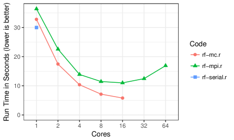
Figure 5: Random forest benchmark on the Oak Ridge National Laboratory machine Rhea.

We see that for one core, the serial implementation is a bit faster than both parallel implementations. This is not too surprising, since one can readily see by comparing Figures 2, 3, and 4 that the parallel versions have additional computational overhead. However, as we increase the number of cores, the run times begin to drop proportionally, up until about 16 cores. Perhaps the “best” run, in the sense of performance improvement per core added, is achieved at 8 cores for both parallel codes. But certainly the performance improves up to 16 cores. The problem is fairly small for the larger core counts. Essentially, the parallel versions begin to run out of work at about 8 cores, but a little more performance can be squeezed out of 16 cores.

The mclapply() parallel version performs slightly better than the MPI version throughout, likely due to somewhat higher overhead involved in MPI communications between R instances compared to forking an R process. This comparison on Rhea would likely persist with a larger problem that does not run out of work at 16 cores, however the MPI version would be able to use more nodes than mclapply() and continue to scale to eventually produce lower run times. Optimally, one would write a third parallel version that would combine the two approaches, giving optimal scaling within nodes with mclapply together with the ability to solve larger problems that need the combined memory of multiple nodes with pbdMPI package. We leave this challenge to the reader as the next step before considering more complex algorithms that rely on scalable matrix computations supported by the pbdR project (Ostrouchov et al., 2012).

References

- Breiman [2001] L. Breiman. Statistical modeling: The two cultures (with comments and a rejoinder by the author). Statist. Sci., 16(3):199–231, 08 2001. doi: 10.1214/ss/1009213726.
- Chen et al. [2012] W.-C. Chen, G. Ostrouchov, D. Schmidt, P. Patel, and H. Yu. pbdMPI: Programming with big data – interface to MPI, 2012. R Package, URL http://cran.r-project.org/package=pbdMPI.
- Eddy and Schervish [1987] W. F. Eddy and M. J. Schervish. Parallel processing on a network of vaxes with applications. In Proceedings of the Statistical Computing Section, pages 41–47. American Statistical Association, 1987.
- Frey and Slate [1991] P. Frey and D. Slate. Letter recognition using holland-style adaptive classifiers. Machine Learning, 6(2):161–182, 1991. ISSN 0885-6125. doi: 10.1007/BF00114162. URL http://dx.doi.org/10.1007/BF00114162.
- Heath [1987] M. Heath, editor. Hypercube Multiprocessors 1987: Proceedings of the Second Conference on Hypercube Multiprocessors. SIAM, 1987. URL http://books.google.com/books?id=fEbjEWonG0UC.
- Leisch and Dimitriadou [2010] F. Leisch and E. Dimitriadou. mlbench: Machine Learning Benchmark Problems, 2010. R package v 2.1-1.
- Liaw and Wiener [2002] A. Liaw and M. Wiener. Classification and regression by randomForest. R News, 2(3):18–22, 2002. URL http://CRAN.R-project.org/doc/Rnews/.
- Matloff [2015] N. Matloff. Parallel Computing for Data Science: With Examples in R, C++ and CUDA. Chapman & Hall/CRC The R Series. CRC Press, 2015. ISBN 9781466587038.
- Message Passing Interface Forum [2015] Message Passing Interface Forum. MPI: A message-passing interface standard version 3.1. 2015. URL http://www.mpi-forum.org.
- Ortega et al. [1989] J. Ortega, G. Voight, and C. Romine. Bibliography on parallel and vector numerical algorithms, 1989. URL http://liinwww.ira.uka.de/bibliography/Parallel/ovr.html.
- Ostrouchov [1987] G. Ostrouchov. Parallel computing on a hypercube: An overview of the architecture and some applications. In M. Heiberger, editor, Proc. 19th Symp. on the Interface of Computer Science and Statistics, pages 27–32, Washington, D.C., 1987. American Statistical Association.
- Ostrouchov et al. [2012] G. Ostrouchov, W.-C. Chen, D. Schmidt, and P. Patel. Programming with big data in R, 2012. URL http://pbdr.org/.
- Schervish [1988] M. J. Schervish. Applications of parallel computation to statistical inference. Journal of the American Statistical Association, pages 976–983, 1988.
- Schmidberger et al. [2009] M. Schmidberger, M. Morgan, D. Eddelbuettel, H. Yu, L. Tierney, and U. Mansmann. State of the art in parallel computing with r. Journal of Statistical Software, 31(1):1–27, 2009.
- Schmidt et al. [2017] D. Schmidt, W.-C. Chen, M. A. Matheson, and G. Ostrouchov. Programming with BIG data in R: Scaling analytics from one to thousands of nodes. Big Data Research, 8:1–11, 2017. ISSN 2214-5796. doi: https://doi.org/10.1016/j.bdr.2016.10.002.
- Wang et al. [2015] C. Wang, M.-H. Chen, E. Schifano, J. Wu, and J. Yan. Statistical methods and computing for big data. arXiv.org, 2015. URL http://arxiv.org/abs/1502.07989v2.
- Xenopoulos et al. [2016] P. Xenopoulos, J. Daniel, M. Matheson, and S. Sukumar. Big data analytics on hpc architectures: Performance and cost. In 2016 IEEE International Conference on Big Data, pages 2286–2295, Dec 2016.