Self-dual effective compact and true compacton configurations in generalized Abelian Higgs models

Abstract

We have studied the existence of self-dual effective compact and true compacton configurations in Abelian Higgs models with generalized dynamics. We have named of an effective compact solution the one whose profile behavior is very similar to the one of a compacton structure but still preserves a tail in its asymptotic decay. In particular we have investigate the electrically neutral configurations of the Maxwell-Higgs and Born-Infeld-Higgs models and the electrically charged ones of the Chern-Simons-Higgs and Maxwell-Chern-Simons-Higgs models. The generalization of the kinetic terms is performed by means of dielectric functions in gauge and Higgs sectors. The implementation of the BPS formalism without the need to use a specific Ansatz has leaded us to the explicit determination of the dielectric function associated to the Higgs sector to be proportional to $\lambda|\phi|^{2\lambda-2}$, $\lambda>1$. Consequently, the followed procedure allows us to determine explicitly new families of self-dual potentials for every model. We have also observed that for sufficiently large values of $\lambda$ every model supports effective compact vortices. The true compacton solutions arising for $\lambda=\infty$ are analytical. Therefore, this new self-dual structures enhance the space of BPS solutions of the Abelian Higgs models and they probably will imply in interesting applications in physics and mathematics.

I Introduction

Topological defects produced by field theories including generalized kinematic terms have been an issue of great interest in the latest years. Usually these models include higher derivatives dynamic terms, but sometimes the generalizations is caused by the introduction of some generalized parameter or functional in the kinetic terms. These modified theories named as k-theories arose initially as effective cosmological models for inflationary evolution Kinflation . Later the k-theories were permeating other issues of field theory and cosmology such as: dark matter DarkMatter , strong gravitational waves Gwaves , the tachyon matter problem 12 and ghost condensates 13 . It is worth emphasizing the possibility that these theories can arise naturally within the context of string theory. Several studies concerning its topological structure have shown k-theories support topological soliton both in models of matter as in gauged models BAi ; SG ; SG1 , in general, they can present some new characteristics when compared those of the usual ones B .

Compactons were defined as solitons with finite wavelength in the pioneer work AM and so far they have been the subject of several studies, since models containing topological defects have been used to represent particles and cosmological objects such as cosmic strings NO . A particular arrangement of particles can be represented with a group of compactons and in this case we will not have the problem of the superposition of particles (or defects) due that compactons do not carry a “tail” in its asymptotic decay. We also point out that compact vortices and skyrmions are intrinsically connected with recent advances in the miniaturization of magnetic materials at the nanometric scale for spintronic applications Jub ; Fert ; Romming . Compact topological defects have gained greater attention as effective low-energy models for QCD concerning skyrmions, where non-perturbative results at the classic level have been reached Sanchez-Guillen . Compact solutions were also successfully employed in the description of boson stars Boson stars and in baby Skyrme models BSKY1 ; BSKY2 .

At the classical level there is a widely employed mechanism to achieve field equations, namely the Bogomol’nyi-Prasad-Sommerfield (BPS) formalism BPS . The BPS method consists in building a set of first-order differential equations which solve as well the second-order Euler-Lagrange equations. One interesting aspect of this mechanism is that all the equations are build up for static field configurations. As a consequence, the first-order equations of motion coming out from the BPS formalism describe field configurations minimizing the total system energy. The static characteristic of the fields in the BPS limit have been applied to investigate topological defects in several frameworks. For example, in the context of planar gauge theories, vortices structures arise from the BPS equations, specially, magnetic vortices were found in Maxwell-Higgs electrodynamics NO . Also we can mention the Chern-Simons-Higgs electrodynamics cshv and mcshv the Maxwell-Chern-Simons-Higgs model both describing electrically charged magnetic vortices. Other interesting framework involving first-order BPS solutions are the nonlinear sigma models (NL$\sigma$M) polyakov in the presence of a gauge field. These theories have been widely applied in the study of field theory and condensed matter physics CMP . We can mention in this sense, the topological defects in a $O(3)$ nonlinear sigma model with the Maxwell term, as it is shown in schroers ; mukherjee2 . Concerning the Chern-Simons term, topological and nontopological defects were analyzed in ghosh ; mukherjee1 . As well the gauged $O(3)$ sigma model with both, Maxwell and the Chern-Simons terms was studied in Refs. sigmaMCSH1 ; sigmaMCSH2 .

The existence of vortex solutions with compact-like profiles in $k$-generalized Abelian Maxwell-Higgs model were studied in Ref. D1 ; D1x and in $k$-generalized Born-Infeld model D2 , however, only in Ref. D1x was found first-order vortices with compact-like profiles. Therefore, the aim of this manuscript is to study the topological vortices engendered by the self-dual configurations obtained from the generalization of the following Abelian Higgs models: Maxwell-Higgs (MH), Born-Infeld-Higgs (BIH), Chern-Simons-Higgs (CSH) and Maxwell-Chern-Simons-Higgs (MCSH). Firstly, we have performed a consistent implementation of the Bogomol’nyi method for every model and obtained the respective generalized self-dual or BPS equations. The developing of the BPS formalism has allowed to fix the form of the function $\omega(|\phi|)$ -composing the generalized term $\omega(|\phi|)|D_{\mu}\phi|^{2}$- which only can be proportional to $\lambda|\phi|^{2\lambda-2}$ for $\lambda>1$ (a similar result was obtained in Ref. L2 ). Secondly, we use the usual vortex Ansatz to obtain the self-dual equations describing axially symmetric configurations. We have observed that independently of the model an effective compact behavior of the vortices arises for a sufficiently large value of the parameter $\lambda$ and only in the limit $\lambda\rightarrow\infty$ the true compacton structures are achieved. Finally, we give our remarks and conclusions.

II The Maxwell-Higgs case

The Maxwell-Higgs model is a classical field theory where the gauge field dynamics is controlled by the Maxwell term and the matter field is represented by the complex scalar Higgs field. The model presents vortex solutions when it is endowed with a fourth-order self-interacting potential promoting a spontaneous symmetry breaking. Although the model seems very simple it presents characteristics very similar to the phenomenological Ginzburg-Landau model for superconductivity Abrikosov or superfluidity in He⁴. The applications of the Maxwell-Higgs model extend from the condensed matter to inflationary cosmology Vilenkin or as an effective field theory for cosmic strings NO .

The generalized Maxwell-Higgs model Bazeia1 is described by the following Lagrangian density

$$\mathcal{L}=-\frac{G(|\phi|)}{4}F_{\mu\nu}F^{\mu\nu}+\omega(|\phi|)|D_{\mu}\phi|^{2}-V(|\phi|)~{}.$$ (1)

The nonstandard dynamics is introduced by two non-negative functions $G(|\phi|)$ and $\omega(|\phi|)$ depending of the Higgs field. The Greek index running from $0$ to $2$. The vector $A_{\mu}$ is the electromagnetic field, the Maxwell strength tensor is $F_{\mu\nu}=\partial_{\mu}A_{\nu}-\partial_{\nu}A_{\mu}$, and $D_{\mu}\phi$ defines the covariant derivative of the Higgs field $\phi$,

$$D_{\mu}\phi=\partial_{\mu}\phi-ieA_{\mu}\phi.$$ (2)

The function $V(|\phi|)$ is a self-interacting scalar potential.

From (1), the gauge field equation reads

$$\partial_{\nu}\left(GF^{\nu\mu}\right)=e\omega J^{\mu},$$ (3)

where $\omega J^{\mu}$ is the conserved current density, i.e., $\partial_{\mu}(\omega J^{\mu})=0$, and $J^{\mu}$ is the usual current density

$$J^{\mu}=i[\phi(D^{\mu}\phi)^{\ast}-\phi^{\ast}(D^{\mu}\phi)].$$ (4)

Along the remain of the section, we are interested in time-independent soliton solutions that ensure the finiteness of the action engendered by (1). Then, from Eq. (3), we read the static Gauss law

$$\partial_{k}\left(G\partial_{k}A_{0}\right)=2e^{2}\omega A_{0}\left|\phi\right|^{2},$$ (5)

and the respective Ampère law

$$\epsilon_{kj}\partial_{j}\left(GB\right)=e\omega J_{k}.$$ (6)

It is clear from the Gauss law that $e\omega J_{0}$ stands for the electric charge density, so that the total electric charge of the configurations is

$$Q=2e^{2}\int d^{2}x\,\omega A_{0}|\phi|^{2}.$$ (7)

which is shown to be null ($Q=0$) by integration of the Gauss law under suitable boundary conditions for the fields at infinity, i.e., $A_{0}\rightarrow 0$, $\phi\rightarrow cte$ and $G(|\phi|)$ a well behaved function. Therefore, the field configurations will be electrically neutral, like it happens in the usual Maxwell-Higgs model.

The fact the configurations being electrically neutral is compatible with the gauge condition, $A_{0}=0,$ which satisfies identically the Gauss law (5). With the choice $A_{0}=0$, the static and electrically neutral configurations are described by the Ampère law (6) and the reduced equation for the Higgs field

$$D_{k}\left(\omega D_{k}\phi\right)-\frac{1}{2}B^{2}\frac{\partial G}{\partial\phi^{\ast}}-\frac{\partial\omega}{\partial\phi^{\ast}}|D_{k}\phi|^{2}-\frac{\partial V}{\partial\phi^{\ast}}=0~{}.$$ (8)

To implement the BPS formalism, we first establish the energy for the static field configuration in the gauge $A_{0}=0$, so it reads

$$E=\int\!d^{2}x\!\left[\frac{G}{2}B^{2}+\omega|D_{k}\phi|^{2}+V\right].$$ (9)

To proceed, we need the fundamental identity

$$|D_{i}\phi|^{2}=|D_{\pm}\phi|^{2}\pm eB|\phi|^{2}\pm\frac{1}{2}\epsilon_{ik}\partial_{i}J_{k}~{},$$ (10)

where $D_{\pm}\phi=D_{1}\phi\pm iD_{2}\phi$. With it, the energy (9) is written as being

$$E = \int\!d^{2}x\left[\frac{G}{2}B^{2}+V(|\phi|)+\omega|D_{\pm}\phi|^{2}\right.$$

$$~{}\ \ \ \ \ \ \ \ \left.\pm e\omega B\left|\phi\right|^{2}\pm\frac{1}{2}\omega\epsilon_{ik}\partial_{i}J_{k}\right]~{}.$$

We observe the term $\omega\epsilon_{ik}\partial_{i}J_{k}$ precludes the implementation of the BPS procedure, i.e,  to express the integrand as a sum of squared terms plus a total derivative plus a term proportional to the magnetic field. This inconvenience already was observed in AHEP-CASANA , such a problem was circumvented by analyzing only axially symmetric solutions in polar coordinates.

The key question about the functional form of $\omega(|\phi|)$ allowing a well defined implementation of the BPS formalism was solved in Ref. L2 . In the following we reproduce some details of the looking for the function $\omega(|\phi|)$. The starting point is the following expression:

$$\omega\epsilon_{ik}\partial_{i}J_{k}=\epsilon_{ik}\partial_{i}(\omega J_{k})-\epsilon_{ik}(\partial_{i}\omega)J_{k}.$$ (12)

By considering $\omega$ be a explicit function of $|\phi|^{2}$, after some algebraic manipulations, the last term $\epsilon_{ik}(\partial_{i}\omega)J_{k}$ becomes expressed as

$$\epsilon_{ik}(\partial_{i}\omega)J_{k}=\left|\phi\right|^{2}\frac{\partial\omega}{\partial\left|\phi\right|^{2}}\epsilon_{ik}\partial_{i}J_{k}+2eB\left|\phi\right|^{4}\frac{\partial\omega}{\partial\left|\phi\right|^{2}}~{},$$ (13)

which after substituted in Eq. (12) allows to obtain

$$\left(\omega+|\phi|^{2}\frac{\partial\omega}{\partial|\phi|^{2}}\right)\epsilon_{ik}\partial_{i}J_{k}=\epsilon_{ik}\partial_{i}(\omega J_{k})-2eB|\phi|^{4}\frac{\partial\omega}{\partial|\phi|^{2}}~{}.$$ (14)

At this point, we establish the function $\omega$ to satisfy the following condition:

$$\omega+\left|\phi\right|^{2}\frac{\partial\omega}{\partial\left|\phi\right|^{2}}=\lambda\omega,~{}\lambda>0,$$ (15)

whose solutions provides the explicit functional form of $\omega(|\phi|)$ to be

$$\omega(|\phi|)=\lambda\frac{|\phi|^{2\lambda-2}}{v^{2\lambda-2}},$$ (16)

it will guarantee that the vacuum expectation value of the Higgs field be $|\phi|=v$.

With the key condition (15), the Eq. (14) allows to express the term $\omega\epsilon_{ik}\partial_{i}J_{k}$ in the following way

$$\omega\epsilon_{ik}\partial_{i}J_{k}=\frac{1}{\lambda}\epsilon_{ik}\partial_{i}\left(\omega J_{k}\right)-2ev^{2}\left(\lambda-1\right)\frac{|\phi|^{2\lambda}}{v^{2\lambda}}B.$$ (17)

By putting the expression (17) in the energy (II), it becomes

$$E = \int\!d^{2}x\,\left[\frac{G}{2}B^{2}+V(|\phi|)+\omega|D_{\pm}\phi|^{2}\right.$$

$$\hskip 35.56593pt\left.\pm ev^{2}\frac{|\phi|^{2\lambda}}{v^{2\lambda}}B\pm\frac{1}{2\lambda}\epsilon_{ik}\partial_{i}\left(\omega J_{k}\right)\right].$$

We now manipulate the two first terms in such a form the energy can be written as

$$E = \int\,\,d^{2}x\left[\frac{G}{2}\left(B\mp\sqrt{\frac{2V}{G}}\right)^{2}+\omega|D_{\pm}\phi|^{2}\right.$$

$$\left.\pm B\left(\sqrt{2GV}+ev^{2}\frac{|\phi|^{2\lambda}}{v^{2\lambda}}\right)\pm\frac{1}{2\lambda}\epsilon_{ik}\partial_{i}\left(\omega J_{k}\right)\right].$$

With the objective the integrand to have a term proportional to the magnetic field, we impose that the factor multiplying it be a constant, i.e.,

$$\sqrt{2GV}+ev^{2}\frac{|\phi|^{2\lambda}}{v^{2\lambda}}=ev^{2}.$$ (20)

Consequently, the self-dual potential $V(|\phi|)$ becomes

$$V(|\phi|)=\frac{1}{G}U^{(\lambda)}(|\phi|),$$ (21)

where we have defined the potential $U^{(\lambda)}(|\phi|)$ given by

$$U^{(\lambda)}(|\phi|)=\frac{e^{2}v^{4}}{2}\left(1-\frac{|\phi|^{2\lambda}}{v^{2\lambda}}\right)^{2}.$$ (22)

We can note that for $\lambda=1$ it becomes the self-dual potential of the Maxwell-Higgs model.

Hence, the energy (92) reads

$$E = \int\!\!d^{2}x\Bigg{\{}\!\!\pm ev^{2}B+\omega|D_{\pm}\phi|^{2}$$

$$\hskip 28.45274pt+\frac{G}{2}\left(B\mp\frac{\sqrt{2U^{(\lambda)}}}{G}\right)^{2}\pm\frac{1}{2\lambda}\epsilon_{ik}\partial_{i}(\omega J_{k})\!\Bigg{\}}.$$

Now by imposing appropriate boundary conditions, the contribution to the total energy of the total derivative is null and the energy has a lower bound proportional to the magnitude of the magnetic flux,

$$E\geq\pm ev^{2}\!\!\int\!\!d^{2}xB=ev^{2}|\Phi|~{},$$ (24)

where for positive flux we choose the upper signal, and for negative flux we choose the lower signal.

The lower bound is saturated by fields satisfying the first-order Bogomol’nyi or self-dual equations BPS

$$D_{\pm}\phi=0,$$ (25)

$$B=\pm\frac{ev^{2}}{G}\left(1-\frac{|\phi|^{2\lambda}}{v^{2\lambda}}\right).$$ (26)

The function $G(|\phi|)$ must be a function providing a finite magnetic field such that $B(|\vec{x}|\rightarrow\infty)\rightarrow 0$ sufficiently rapid to provide a finite total magnetic flux.

In the BPS limit the energy (9) provides the energy density of the self-dual configurations

$$\varepsilon_{{}_{BPS}}=\frac{2U^{(\lambda)}}{G}+\lambda\frac{|\phi|^{2\lambda-2}}{v^{2\lambda-2}}\left|D_{k}\phi\right|^{2},$$ (27)

it will be finite and positive-definite for $\lambda>0$. We here also require the function $G(|\phi|)$ yielding a finite BPS energy density such that $\varepsilon_{{}_{BPS}}(|\vec{x}|\rightarrow\infty)\rightarrow 0$ sufficiently rapid to provide a finite total energy.

II.1 Maxwell-Higgs effective compact vortices for $\lambda$ finite

In the following, with loss of generality, we have chosen $G(|\phi|)=1$ (for this one and for all other models analyzed along the manuscript) with the aim to study the influence of the generalized dynamic in Higgs sector in the formation of effective compact vortices and true compactons. Such a generalization provided by the function $\omega(|\phi|)$ defined in Eq. (16) and its effects in the formation of effective compact vortices apparently remains unexplored in the literature.

Thus, we seek axially symmetric solutions according to the usual vortex Ansatz NO

$$\phi(r,\theta)=vg(r)e^{in\theta},\quad A_{\theta}(r)=-\frac{a(r)-n}{er},$$ (28)

with $n=\pm 1,\pm 2,\pm 3...$ standing for the winding number of the vortex solutions.

The profiles $g(r)$ and $a(r)$ are regular functions describing solutions possessing finite energy and obeying the boundary conditions,

$$g(0) = 0,\;\;a(0)=n,$$ (29)

$$g(\infty) = 1\text{{,}}\;\;a(\infty)=0.$$ (30)

Under the Ansatz (28), the magnetic field reads

$$B(r)=-\frac{1}{er}\frac{da}{dr}.$$ (31)

The correspondent quantized magnetic flux is given by

$$\Phi=\int\!d^{2}xB=\frac{2\pi}{e}n,$$ (32)

as expected.

The BPS equations (25) and (26) are written as

$$g^{\prime} = \pm\frac{ag}{r},$$ (33)

$$-\frac{a^{\prime}}{r} = \pm e^{2}v^{2}(1-g^{2\lambda}).$$ (34)

The upper (lower) signal corresponds to the vortex (antivortex) solution with winding number $n>0$ ($n<0$).

The self-dual energy density (27) is expressed by

$$\varepsilon_{{}_{BPS}}=e^{2}v^{4}\left(1-g^{2\lambda}\right)^{2}+2\lambda v^{2}g^{2\lambda-2}\left(\frac{ag}{r}\right)^{2}.$$ (35)

It will be finite and positive-definite for $\lambda\geq 1$.

The total energy of the self-dual solutions is given by the lower bound (24),

$$E_{{}_{BPS}}=\pm ev^{2}\Phi_{B}=\pm 2\pi v^{2}n,$$ (36)

it is proportional to the winding number of the vortex solution, as expected.

The behavior of $g(r)$ and $a(r)$ near the boundaries can be easily determined by solving the self-dual equations (33) and (34) around the boundary conditions (29) and (30). Then, for $r\rightarrow 0$, the profiles behave as

$$g(r) \approx C_{n}r^{n}+...$$ (37)

$$a(r) \approx n-\frac{e^{2}v^{2}}{2}r^{2}+...$$ (38)

where the constant $C_{n}>0$ is computed numerically.

On the other hand, when $r\rightarrow\infty$, they behave as

$$g(r) \approx 1-\frac{C_{\infty}}{\sqrt{r}}e^{-mr},$$ (39)

$$a(r) \approx mC_{\infty}\sqrt{r}e^{-mr},$$ (40)

the constant $C_{\infty}$ is determined numerically and $m$, the self-dual mass, is given by

$$m=ev\sqrt{2\lambda},$$ (41)

remembering that $ev\sqrt{2}$ is the mass scale of the usual Maxwell-Higgs model. The influence of the generalization in the mass scale explains the changes in the vortex-core size for large values of $\lambda$ observed in the Figs. 1 and 2.

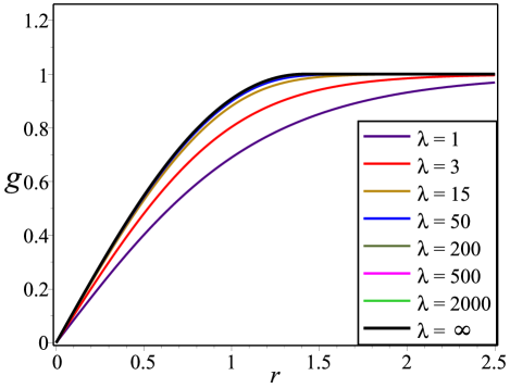
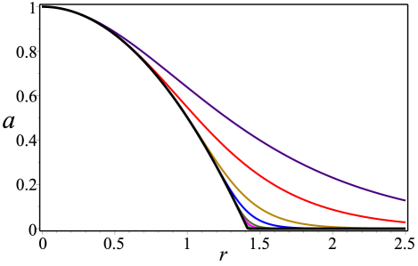
Figure 1: The profiles $g(r)$ (upper) and $a(r)$ (lower) coming from generalized Maxwell-Higgs model (1) with $G(g)=1$ and $\omega(g)=\lambda g^{2\lambda-2}$. Observe that $\lambda=1$ (indigo lines) represents the usual MH model and the true compacton solution is given by $\lambda=\infty$ (black lines).

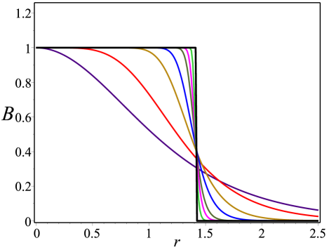
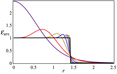
Figure 2: The magnetic field $B(r)$ (upper) and the BPS energy density $\varepsilon_{{}_{BPS}}(r)$ (lower) coming from generalized Maxwell-Higgs model (1) with $G(g)=1$ and $\omega(g)=\lambda g^{2\lambda-2}$. Observe that $\lambda=1$ (indigo lines) represents the usual MH model and the true compacton solution is given by $\lambda=\infty$ (black lines).

II.2 Maxwell-Higgs compactons for $\lambda=\infty$

By considering the profile $0\leq g(r)<1$, in the limit $\lambda\rightarrow\infty$ the potential (22) acquires the following form

$$U^{(\infty)}(g)=\frac{e^{2}v^{4}}{2}\Theta(1-g),$$ (42)

where $\Theta(1-g)$ is the Heaviside function.

The BPS equations (33) and (34), in the limit $\lambda\rightarrow\infty$ are written as

$$g^{\prime} = \pm\frac{ag}{r},$$ (43)

$$-\frac{a^{\prime}}{r} = \pm e^{2}v^{2}\Theta(1-g).$$ (44)

The boundary conditions for compacton solutions are

$$g(0) = 0,\;\;a(0)=n,$$ (45)

$$g(r) = 1,\;\;a(r)=0,\;r_{c}\leq r<\infty.$$ (46)

The radial distance $r_{c}<\infty$ is the value where the profile $g(r)$ reaches the vacuum value and the gauge field profile $a(r)$ becomes null.

The solutions (for $n>0$) of the compacton BPS equations (43) and (44) provides analytical profiles for the Higgs and gauge field,

$$g^{(\infty)}(r) = \left(\frac{r}{r_{c}}\right)^{n}\exp\left[\frac{n}{2}\left(1-\frac{r^{2}}{r_{c}^{2}}\right)\right]\Theta(r_{c}-r)$$

$$+\Theta(r-r_{c}),$$

$$a^{(\infty)}(r) = n\left(1-\frac{r^{2}}{r_{c}^{2}}\right)\Theta({r_{c}}-{r}),$$ (48)

where the radial distance $r_{c}$ is given by

$$r_{c}=\frac{\sqrt{2n}}{\left|ev\right|}.$$ (49)

The magnetic field and BPS energy density of the Maxwell-Higgs compacton are

$$B^{(\infty)}(r) = ev^{2}\Theta(r_{c}-r),$$ (50)

$$\varepsilon_{{}_{BPS}}^{(\infty)}(r) = e^{2}v^{4}\Theta(r_{c}-r).$$ (51)

The numerical solutions (for all model analyzed in the manuscript) were performed using the routines for boundary value problems of the software Maple 2015. We have chosen the upper signals in BPS equations (33) and (34). We have fixed $e=v=1$, the winding number $n=1$ and calculated the numerical solutions for some finite values of $\lambda$. The profiles for the Higgs and gauge fields are given in Fig. 1 and, the correspondent ones for the magnetic field and the self-dual energy density are depicted in Fig. 2.

The numerical analysis shows that for sufficiently large but finite values of $\lambda$, the profiles are very alike to compacton solution ones, we have named them Maxwell-Higgs effective compact vortices. The true Maxwell-Higgs compacton is formed when $\lambda=\infty$ (see black line profiles in Figs. 1 and 2).

III The Born-Infeld-Higgs case

The Born-Infeld theory is a nonlinear electrodynamic that was introduced to remove the divergence of the electron self-energy BI . It is the only completely exceptional nonlinear electrodynamics because to the absence of shock waves and birefringence in its propagation properties Boillat . Concerning topological defects in the Born-Infeld-Higgs model, vortex solutions were found in BI-VORTEX . One generalization of BIH model was firstly done in D2 but no self-dual solutions were found. On the other hand, the self-dual or BPS topological vortex solutions were found in a generalized Born-Infeld-Higgs model introduced in Ref. Casana .

The Lagrangian density of our ($2+1$)-dimensional theory is written as

$$\mathcal{L}=\beta^{2}\left(1-\mathcal{R}\right)+\omega\left(\left|\phi\right|\right)\left|D_{\mu}\phi\right|^{2}-W\left(\left|\phi\right|\right)\text{,}$$ (52)

where we go to consider the function $\omega\left(\left|\phi\right|\right)$ given by Eq. (16). We have also defined the following functions

$$\mathcal{R} = \sqrt{1+\frac{G\left(\left|\phi\right|\right)}{2\beta^{2}}F_{\mu\nu}F^{\mu\nu}},$$ (53)

$$W\left(\left|\phi\right|\right) = \beta^{2}\left[1-V\left(\left|\phi\right|\right)\right].$$ (54)

The generalized potential $W\left(\left|\phi\right|\right)$, a nonnegative function, inherits its structure from the function $V(|\phi|)$, which is restricted by the condition $0<V(|\phi|)\leq 1$, so $W(\phi)>0$. The Born-Infeld parameter $\beta$, provides modified dynamics for both scalar and gauge fields further enriching the family of possible models.

From the action (52) the gauge field equation of motion reads

$$\partial_{\nu}\left(\frac{G}{\mathcal{R}}F^{\nu\mu}\right)=e\omega J^{\mu}.$$ (55)

We are interested in stationary solutions, so the Gauss law becomes

$$\partial_{j}\left(\frac{G}{\mathcal{R}}\partial_{j}A_{0}\right)=2\omega e^{2}A_{0}\left|\phi\right|^{2}.$$ (56)

Similarly to it happens in Maxwell-Higgs model, the field configurations are electrically neutral therefore we go to work in the gauge $A_{0}=0$.

Consequently, at static regime, in the gauge $A_{0}=0$, the Ampère law is given by

$$\epsilon_{kj}\partial_{j}\left(\frac{G}{\mathcal{R}}B\right)-e\omega J_{k}=0,$$ (57)

and the Higgs field equation reads

$$0 = \omega\left(D_{j}D_{j}\phi\right)+\left(\partial_{j}w\right)D_{j}\phi$$

$$-\frac{\partial\omega}{\partial\phi^{\ast}}\left|D_{j}\phi\right|^{2}-\frac{B^{2}}{\ 2\mathcal{R}}\frac{\partial G}{\partial\phi^{\ast}}-\frac{\partial W}{\partial\phi^{\ast}}.$$

In the last two equations $\mathcal{R}$ reads

$$\mathcal{R}=\left(1+\frac{G}{\beta^{2}}B^{2}\right)^{1/2}.$$ (59)

The energy of the system, in static regime and in the gauge $A_{0}=0$, is given by

$$E=\int\!d^{2}x\left[\beta^{2}\left(\mathcal{R}-V\right)+\omega\left|D_{k}\phi\right|^{2}\right],$$ (60)

and will be nonnegative whenever the condition $\mathcal{R}\geq V$ is satisfied.

To proceed with the BPS formalism, we use the identities (10) and (17) such that the Eq. (60) becomes

$$E = 2\pi\!\int\!d^{2}x\Bigg{[}\pm ev^{2}B+\omega|D_{\pm}\phi|^{2}\pm\frac{1}{2\lambda}\epsilon_{ik}\partial_{i}\left(\omega J_{k}\right)$$

$$\hskip 42.67912pt+\frac{\mathcal{R}}{2G}\left(\frac{G}{\mathcal{R}}B\mp\sqrt{2U^{(\lambda)}}\right)^{2}$$

$$\hskip 42.67912pt+\beta^{2}\left(\mathcal{R}-V\right)-\frac{1}{2}\frac{GB^{2}}{\mathcal{R}}-\frac{\mathcal{R}}{G}U^{(\lambda)}\Bigg{]}.$$

We have introduced the potential $U^{(\lambda)}(|\phi|)$ given by Eq. (22) with the aim to obtain the term proportional to the magnetic field $ev^{2}B$.

The Bogomol’nyi procedure would be complete if we require that the third row in (III) to be null, so we obtain

$$V+\frac{\mathcal{R}U^{(\lambda)}}{\beta^{2}G}=\frac{1}{2}\mathcal{R}+\frac{1}{2\mathcal{R}}.$$ (62)

It provides a relation between the functions $V$, $G$ and $\mathcal{R}$. We here clarify that the Eq. (62) it is not arbitrary because, as we will observe later, in the BPS limit it becomes equivalent to the condition on the diagonal components of the energy-momentum tensor $T_{\mu\nu}$: $T_{11}+T_{22}=0$, proposed by Schaposnik and Vega Scha to obtain self-dual configurations.

Then, the condition (62) allows to write the energy (60) in the Bogomol’nyi form,

$$E = \int\!\!d^{2}x\left\{\omega|D_{\pm}\phi|^{2}+\frac{\mathcal{R}}{2G}\left(\frac{G}{\mathcal{R}}B\mp\sqrt{2U^{(\lambda)}}\right)^{2}\right.$$ (63)

$$\hskip 28.45274pt\pm ev^{2}B\pm\frac{1}{2\lambda}\epsilon_{ik}\partial_{i}\left(\omega J_{k}\right)\Bigg{\}}.$$

Under suitable boundary conditions, the integration of the total derivative in Eq. (63) gives null contribution to the energy. Hence, it becomes clear that the energy possess a lower bound

$$E\geq ev^{2}\left|\Phi\right|,$$ (64)

with $\Phi$ the total magnetic flux. Such a lower bound is saturated when the fields satisfy the BPS or self-dual equations

$$D_{\pm}\phi=0,$$ (65)

$$\frac{G}{\mathcal{R}}B=\pm ev^{2}\left(1-\frac{\left|\phi\right|^{2\lambda}}{v^{2\lambda}}\right).$$ (66)

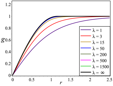
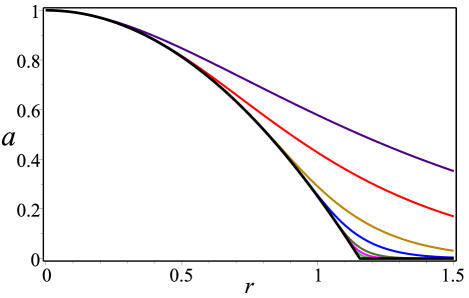
Figure 3: The profiles $g(r)$ (upper) and $a(r)$ (lower) coming from the generalized Born-Infeld-Higgs model (52) with $G(g)=1$ and $\omega(g)=\lambda g^{2\lambda-2}$. Observe that $\lambda=1$ (indigo lines) represents the usual BIH model and the true compacton solution is given by $\lambda=\infty$ (black lines).

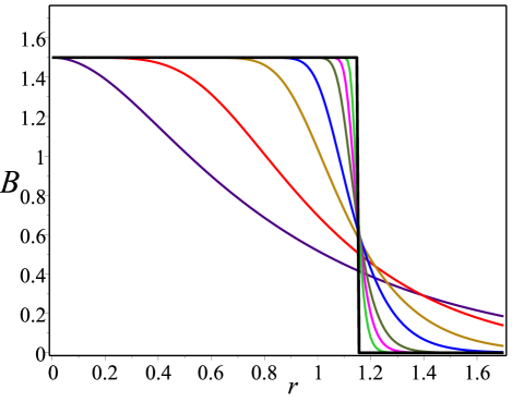
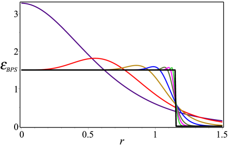
Figure 4: The magnetic field $B(r)$ (upper) and the BPS energy density $\varepsilon_{{}_{BPS}}(r)$ (lower) coming from the generalized Born-Infeld-Higgs model (52) with $G(g)=1$ and $\omega(g)=\lambda g^{2\lambda-2}$. Observe that $\lambda=1$ (indigo lines) represents the usual BIH model and the true compacton solution is given by $\lambda=\infty$ (black lines).

By using the BPS equations in Eq. (62) we compute the self-dual potential $V(|\phi|)$,

$$V=\frac{1}{\mathcal{R}}=\sqrt{1-\frac{2U^{(\lambda)}}{\beta^{2}G}}$$ (67)

This way the second BPS equation (66) becomes

$$B=\pm\frac{ev^{2}}{GV}\left(1-\frac{\left|\phi\right|^{2\lambda}}{v^{2\lambda}}\right).$$ (68)

By using the BPS equations in (60) we find the BPS energy density is given by

$$\varepsilon_{{}_{BPS}}=\frac{2U^{(\lambda)}}{GV}+\lambda\frac{|\phi|^{2\lambda-2}}{v^{2\lambda-2}}\left|D_{k}\phi\right|^{2},$$ (69)

it will be positive-definite $\lambda>0$.

III.1 Born-Infeld-Higgs effective compact vortices for $\lambda$ finite

In Ref. D2 it was explored the existence of effective compact vortex solutions but the self-dual ones were not found. In this section we show the existence of such self-dual effective compact solutions in BIH model. Without loss of generality, we perform the study by considering $G(|\phi|)=1$ in the Lagrangian density (52).

The searching for vortex solutions is made by means of the vortex Ansatz introduced in the Eq. (28). Thus, the BPS equations (65) and (66) read

$$g^{\prime} = \pm\frac{ag}{r},$$ (70)

$$-\frac{a^{\prime}}{r} = \pm\frac{e^{2}v^{2}\left(1-g^{2\lambda}\right)}{\sqrt{1-\displaystyle\frac{e^{2}v^{4}\left(1-g^{2\lambda}\right)^{2}}{\beta^{2}}}},$$ (71)

The behavior of the profiles $g(r)$ and $a(r)$ when $r\rightarrow 0$ is determined by solving the self-dual equations (70) and (71), so we have

$$g(r) \approx C_{n}r^{n}+...,$$ (72)

$$a(r) \approx n-\frac{e^{2}v^{2}\beta}{2\sqrt{\beta^{2}-e^{2}v^{4}}}r^{2}+...,\quad\quad$$ (73)

Similarly, the behavior of the profiles for $r\rightarrow\infty$ is

$$g(r) \approx 1-\frac{C_{\infty}}{\sqrt{r}}e^{-mr},$$ (74)

$$a(r) \approx {m}C_{\infty}\sqrt{r}e^{-mr},$$ (75)

where $m$, the self-dual mass, is given by

$$m=ev\sqrt{2\lambda}$$ (76)

it is exactly the same obtained for the generalized MH model analyzed in the previous section.

The BPS energy density for the self-dual vortices reads

$$\varepsilon_{{}_{BPS}}=\displaystyle\frac{e^{2}v^{4}\left(1-g^{2\lambda}\right)^{2}}{\sqrt{1-\displaystyle\frac{e^{2}v^{4}\left(1-g^{2\lambda}\right)^{2}}{\beta^{2}}}}+2\lambda v^{2}g^{2\lambda-2}\left(\frac{ag}{r}\right)^{2},$$ (77)

it will be positive-definite and finite for $\lambda\geq 1$.

III.2 Born-Infeld-Higgs compactons for $\lambda=\infty$

In the limit $\lambda\rightarrow\infty$, the BPS equations (70) and (71) read

$$g^{\prime} = \pm\frac{ag}{r},$$ (78)

$$-\frac{a^{\prime}}{r} = \pm\frac{e^{2}v^{2}\Theta(1-g)}{\displaystyle\sqrt{1-\frac{e^{2}v^{4}}{\beta^{2}}}},$$ (79)

with the profiles $g(r)$ and $a(r)$ satisfying the boundary conditions (45) and (46).

By solving the BPS compacton equations for the BIH model, we obtain also analytical solutions

$$g^{(\infty)}(r) = \left(\frac{r}{r_{c}}\right)^{n}\exp\left[\frac{n}{2}\left(1-\frac{r^{2}}{r_{c}^{2}}\right)\right]\!\Theta(r_{c}-r)\quad$$

$$+\Theta(r-r_{c}),$$

$$a^{(\infty)}(r) = n\left(1-\frac{r^{2}}{r_{c}^{2}}\right)\Theta\left(r_{c}-r\right),$$ (81)

where the radial distance $r_{c}$ now is given by

$$r_{c}=\frac{\sqrt{2n}}{\left|ev\right|}\left(1-\frac{e^{2}v^{4}}{\beta^{2}}\right)^{1/4}.$$ (82)

The magnetic field and BPS energy density profiles of the Born-Infeld-Higgs compacton are

$$B^{(\infty)}(r) = ev^{2}\left(1-\frac{e^{2}v^{4}}{\beta^{2}}\right)^{-1/2}\Theta(r_{c}-r),$$ (83)

$$\varepsilon_{{}_{BPS}}^{(\infty)}(r) = e^{2}v^{4}\left(1-\frac{e^{2}v^{4}}{\beta^{2}}\right)^{-1/2}\Theta(r_{c}-r).$$ (84)

In order to compute the numerical solutions we choose the upper signs in equations (70) and (71), $e=1$, $v=1$, $\beta=3/\sqrt{5}$ and winding number $n=1$. Similarly to the MH model, the effective compacton behavior appears for sufficiently large values of $\lambda$, see Figs. 3 and 4. The true Born-Infeld-Higgs compacton arising for $\lambda=\infty$ also are depicted (see black line profiles) in Figs. 3 and 4.

IV The Chern-Simons-Higgs case

In this section we apply the same formalism to construct self-dual solutions in the generalized Abelian Chern-Simons-Higgs model. Physics in two spatial dimensions is closely linked to CS theory, which contains theoretical novelties besides practical application in various phenomena of condensed matter, such as the physics of Anyons and it is related with the fractional quantum Hall effect Ezawa . It can be found an extensive literature about CS theory, some of the pioneer papers concerning topological and non-topological solutions as well as relativistic and non-relativistic models can be found in hor ; JW ; JP ; JLW . Also exists a close connection between CS theory and supersymmetry. This connection was firstly demonstrated in LLW , where from a $N=2$ supersymmetric extension of CS model it was found the specific potential for the Bogomol’nyi equations, which arise naturally.

The generalized Chern-Simons-Higgs model is described by the following Lagrangian density

$$\mathcal{L}=\frac{\kappa}{4}\epsilon^{\mu\nu\rho}A_{\mu}F_{\nu\rho}+\omega(|\phi|)|D_{\mu}\phi|^{2}-V(|\phi|),$$ (85)

with the function $\omega\left(\left|\phi\right|\right)$ given by Eq. (16). The gauge field equation to be

$$\frac{\kappa}{2}\epsilon^{\mu\alpha\beta}F_{\alpha\beta}-e\omega J^{\mu}=0~{},$$ (86)

and the Gauss law reads

$$\kappa B=e\omega J_{0}.$$

It is clear that the electric charge density is $e\omega J_{0}$ whose integration performed via the Gauss law gives

$$Q=\int\!d^{2}x\,e\omega J_{0}=\kappa\int\!d^{2}x~{}B=\kappa\Phi.$$ (87)

So such as it happens in usual CSH model, the electric charge is nonnull and proportional to the magnetic so the field configurations always will be electrically charged.

These are the stationary points of the energy which for the static field configuration reads

$$E=\!\!\int\!d^{2}x\!\left[-\kappa A_{0}B-e^{2}\omega A_{0}^{2}|\phi|^{2}+\omega|D_{i}\phi|^{2}+V(|\phi|)\right].$$ (88)

From the static Gauss law, we obtain the relation

$$A_{0}=-\frac{\kappa}{2e^{2}}\frac{B}{\omega|\phi|^{2}},$$ (89)

which substituted in Eq. (88) leads to the following expression for the energy:

$$E=\int\!d^{2}x\left[\frac{\kappa^{2}}{4e^{2}}\frac{B^{2}}{\omega|\phi|^{2}}+\omega|D_{i}\phi|^{2}+V(|\phi|)\right].$$ (90)

We now use the identities (10) and (17) in Eq. (88) such that the energy becomes

$$E = \!\int\!\!d^{2}x\left[\frac{\kappa^{2}}{4e^{2}}\frac{B^{2}}{\omega|\phi|^{2}}+V(|\phi|)+\omega|D_{\pm}\phi|^{2}\right.$$

$$\hskip 35.56593pt\left.\pm ev^{2}\frac{|\phi|^{2\lambda}}{v^{2\lambda}}B\pm\frac{1}{2\lambda}\epsilon_{ik}\partial_{i}\left(\omega J_{k}\right)\right].$$

After some manipulation the energy can be expressed almost in the Bogomol’nyi form

$$E = \!\int\!d^{2}x\left[\frac{\kappa^{2}}{4e^{2}}\frac{1}{|\phi|^{2}\omega}\left(B\mp\frac{2e\left|\phi\right|}{\kappa}\sqrt{\omega V}\right)^{2}\right.$$ (92)

$$\hskip 35.56593pt+\omega|D_{\pm}\phi|^{2}\pm\frac{1}{2\lambda}\epsilon_{ik}\partial_{i}\left(\omega J_{k}\right)$$

$$\hskip 35.56593pt\left.\pm B\left(\frac{\kappa}{e|\phi|}\sqrt{\frac{V}{\omega}}+ev^{2}\frac{|\phi|^{2\lambda}}{v^{2\lambda}}\right)\right]~{}.$$

We observe that the Bogomol’nyi procedure will be complete if the term multiplying the magnetic field is a constant, i.e.,

$$\frac{\kappa}{e|\phi|}\sqrt{\frac{V}{\omega}}+ev^{2}\frac{|\phi|^{2\lambda}}{v^{2\lambda}}=ev^{2},$$ (93)

such a condition allows to determine the self-dual potential $V(|\phi|)$ to be

$$V(|\phi|)=\lambda\frac{e^{4}v^{6}}{\kappa^{2}}\frac{|\phi|^{2\lambda}}{v^{2\lambda}}\left(1-\frac{\left|\phi\right|^{2\lambda}}{v^{2\lambda}}\right)^{2}.$$ (94)

We can see that for $\lambda=1$, the $|\phi|^{6}$-potential of the usual Chern-Simon-Higgs model is recovered.

Hence, the energy (92) reads

$$E = \!\!\int\!d^{2}x\left\{\pm ev^{2}B\pm\frac{1}{2\lambda}\epsilon_{ik}\partial_{i}\left(\omega J_{k}\right)+\omega|D_{\pm}\phi|^{2}\right.\quad$$

$$\hskip 19.91684pt\left.+\frac{\kappa^{2}}{4e^{2}|\phi|^{2}\omega}\left[B\mp\frac{2e^{2}v^{2}}{\kappa^{2}}\lambda\frac{|\phi|^{2\lambda}}{v^{2\lambda}}\sqrt{2U^{(\lambda)}}\right]^{2}\right\}.$$

We see that under appropriated boundary conditions the total derivative gives null contribution to the energy. Then, the energy is bounded below by a multiple of the magnetic flux magnitude

$$E\geq\pm ev^{2}\!\!\int\!\!d^{2}xB=ev^{2}|\Phi|.$$ (96)

This bound is saturated by fields satisfying the first-order Bogomol’nyi or self-dual equations BPS

$$D_{\pm}\phi=0,$$ (97)

$$B=\pm\frac{2e^{3}v^{4}}{\kappa^{2}}\lambda\frac{|\phi|^{2\lambda}}{v^{2\lambda}}\left(1-\frac{\left|\phi\right|^{2\lambda}}{v^{2\lambda}}\right).$$ (98)

In order the magnetic field be nonsingular at origin, it is required that the $\lambda>0$.

By using the BPS equation in (90) we find the energy density is given by

$$\varepsilon_{{}_{BPS}}=2\lambda\frac{e^{4}v^{6}}{\kappa^{2}}\frac{|\phi|^{2\lambda}}{v^{2\lambda}}\left(1-\frac{\left|\phi\right|^{2\lambda}}{v^{2\lambda}}\right)^{2}+\lambda\frac{|\phi|^{2\lambda-2}}{v^{2\lambda-2}}\left|D_{k}\phi\right|^{2},$$ (99)

it will be positive-definite $\lambda>0$.

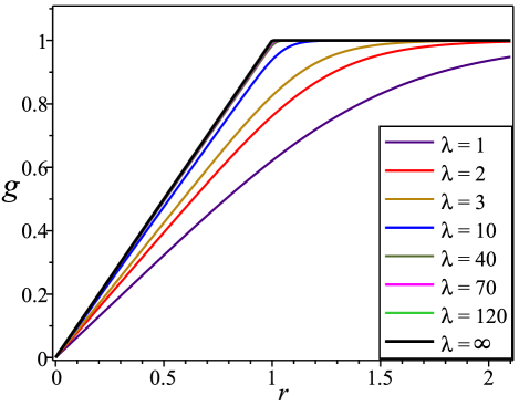
Figure 5: The profiles $g(r)$ (upper) and $a(r)$ (lower) coming from the generalized Chern-Simons-Higgs model (85) with $\omega(g)=\lambda g^{2\lambda-2}$. Observe that $\lambda=1$ (indigo lines) represents the usual CSH model and the true compacton solution is given by $\lambda=\infty$ (vertical black lines representing the $\delta$-Dirac function).

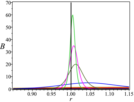
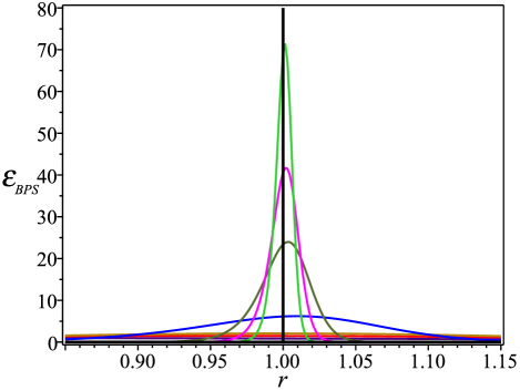
Figure 6: The magnetic field $B(r)$ (upper) and the BPS energy density $\varepsilon_{{}_{BPS}}(r)$ (lower) coming from the generalized Chern-Simons-Higgs model (85) with $\omega(g)=\lambda g^{2\lambda-2}$. Observe that $\lambda=1$ (indigo lines) represents the usual CSH model and the true compacton solution is given by $\lambda=\infty$ (vertical black lines representing the $\delta$-Dirac function).

IV.1 Chern-Simons-Higgs effective compact vortices for $\lambda$ finite

The BPS equations (97) and (98) read

$$g^{\prime} = \pm\frac{ag}{r},$$ (100)

$$-\frac{a^{\prime}}{r} = \pm\frac{2e^{4}v^{4}}{\kappa^{2}}\lambda g^{2\lambda}(1-g^{2\lambda}),$$ (101)

The behavior of $g(r)$ and $a(r)$ near the boundaries can be easily determined by solving the self-dual equations (100) and (101) around the boundary values (29) and (30). Thus, for $r\rightarrow 0$, the profile functions behave as

$$g(r) \approx C_{n}r^{n}+...,$$ (102)

$$a(r) \approx n\mp\frac{\lambda e^{4}v^{4}}{\left(n\lambda+1\right)\kappa^{2}}\left(C_{n}\right)^{2\lambda}r^{2n\lambda+2}+...,$$ (103)

where the constant $C_{n}>0$ is determined only numerically.

On the other hand, when $r\rightarrow\infty$ they behave as

$$g(r) \approx 1-\frac{C_{\infty}}{\sqrt{r}}e^{-mr},$$ (104)

$$a(r) \approx C_{\infty}{m}\sqrt{r}e^{-mr},$$ (105)

with the constant $C_{\infty}$ computed numerically and $m$ being the self-dual mass

$$m=\frac{2\lambda e^{2}v^{2}}{\kappa}.$$ (106)

Observe for $\lambda=1$ it becomes the one of the usual self-dual Chern-Simons-Higgs bosons.

The BPS energy density for the self-dual vortices is given by

$$\varepsilon_{{}_{BPS}}=2\lambda\frac{e^{4}v^{6}}{\kappa^{2}}g^{2\lambda}\left(1-g^{2\lambda}\right)^{2}+2\lambda v^{2}g^{2\lambda-2}\left(\frac{ag}{r}\right)^{2},$$ (107)

and it will be positive-definite and finite for $\lambda\geq 1$.

IV.2 Chern-Simons-Higgs compactons for $\lambda=\infty$

From Eqs. (100) and (101) we obtain the BPS equations for the Chern-Simons-Higgs compactons

$$g^{\prime} = \pm\frac{ag}{r},$$ (108)

$$-\frac{a^{\prime}}{r} = \frac{2e^{4}v^{4}}{\kappa^{2}}\delta(1-g),$$ (109)

with the boundary condition given in Eqs. (45) and (46).

By solving the BPS compacton equations for $n>0$, we obtain the analytic profiles

$$g^{(\infty)}(r) = \left(\frac{r}{r_{c}}\right)^{n}\Theta(r_{c}-r)+\Theta(r-r_{c}),$$ (110)

$$a^{(\infty)}(r) = n\Theta\left(r_{c}-r\right).$$ (111)

The radial distance $r_{c}$ is calculated to be

$$r_{c}=\frac{n\left|\kappa\right|}{e^{2}v^{2}}.$$ (112)

The magnetic field and BPS energy density of the Chern-Simons-Higgs compacton are

$$B^{(\infty)}(r) = \frac{n}{er_{c}}\delta(r_{c}-r),$$ (113)

$$\varepsilon_{{}_{BPS}}^{(\infty)}(r) = \frac{nv^{2}}{r_{c}}\delta(r_{c}-r).$$ (114)

In order to compute the numerical solutions we choose the upper signs in equations (100) and (101), $e=1$, $v=1$, $\kappa=1$ and winding number $n=1$. From the numerical analysis, we can see the appearing of the effective compacton behavior for not very large values of $\lambda$ such it is explicitly shown in Figs. 5 and 6. An interesting feature of the Chern-Simons-Higgs effective compact vortices is the enhancement of the ring shape (inclusive for $n=1$), for increasing values of $\lambda$ in the profiles for the magnetic field and the BPS energy density (see Fig. 6). The analytic CSH compacton structures appearing in $\lambda=\infty$ are represented by the black line profiles in Fig. 5 and 6.

V The Maxwell-Chern-Simons-Higgs case

Electrically charged vortices were first found in the Abelian-Higgs model by S. K. Paul and A. Khare Khare , where the Chern-Simons term was included in the usual Maxwell-Higgs action. This was an ingenious manner to avoid the temporal gauge, $A_{0}\neq 0$, coupling the electric charge density to the magnetic field. This model has also been generalized by multiplying a dielectric (scalar) function in the Maxwell kinetic term Ghosh ; Bazeia2 yielding topological and not topological solutions satisfying a Bogomol’nyi bound.

The generalized Maxwell-Chern-Simons-Higgs model is described by the following Lagrangian density

$$\mathcal{L} = -\frac{G(|\phi|)}{4}F_{\mu\nu}F^{\mu\nu}+\frac{\kappa}{4}\epsilon^{\mu\nu\rho}A_{\mu}F_{\nu\rho}$$

$$+\omega(|\phi|)|D_{\mu}\phi|^{2}+\frac{G(|\phi|)}{2}\partial_{\mu}N\partial^{\mu}N$$

$$-e^{2}\omega(|\phi|)N^{2}|\phi|^{2}-V(|\phi|)~{}.$$

where the function $\omega\left(\left|\phi\right|\right)$ given by Eq. (16). The gauge field equation reads

$$\partial_{\nu}\left(GF^{\nu\mu}\right)+\frac{\kappa}{2}\epsilon^{\mu\alpha\beta}F_{\alpha\beta}-e\omega J^{\mu}=0,$$ (116)

the static Gauss law is

$$\partial_{k}\left(G\partial_{k}A_{0}\right)-\kappa B=2e^{2}\omega A_{0}\left|\phi\right|^{2}.$$ (117)

Similarly, the equation of motion of the Higgs field is

$$0 = D_{\mu}\left(\omega D^{\mu}\phi\right)+\left(\frac{1}{4}F_{\mu\nu}F^{\mu\nu}-\frac{1}{2}\partial_{\mu}N\partial^{\mu}N\right)\frac{\partial G}{\partial\phi^{\ast}}$$ (118)

$$-\frac{\partial\omega}{\partial\phi^{\ast}}|D_{\mu}\phi|^{2}+2e^{2}\omega N|\phi|^{2}+\frac{\partial V}{\partial\phi^{\ast}}~{}.$$

Likewise than previous models, we are interested in time-independent soliton solutions that ensure the finiteness of the action (85). These are the stationary points of the energy which for the static field configuration reads

$$E = \!\!\int\!d^{2}x\!\left[\frac{G}{2}B^{2}+\frac{G}{2}\left(\partial_{j}A_{0}\right)^{2}+e^{2}\omega\left(A_{0}\right)^{2}|\phi|^{2}\right.$$

$$\left.+\omega|D_{j}\phi|^{2}+\frac{G}{2}\left(\partial_{j}N\right)^{2}+e^{2}\omega N^{2}|\phi|^{2}+V(|\phi|)\right].$$

To proceed, we use the identities (10) and (17) such that the energy becomes

$$E = \!\!\int\!d^{2}x\!\left[\frac{G}{2}B^{2}+V(|\phi|)+\frac{G}{2}\left(\partial_{j}A_{0}\right)^{2}+\frac{G}{2}\left(\partial_{j}N\right)^{2}\right.$$

$$+e^{2}\omega\left(A_{0}\right)^{2}|\phi|^{2}+e^{2}\omega N^{2}|\phi|^{2}$$

$$\left.+\omega|D_{\pm}\phi|^{2}\pm ev^{2}\frac{|\phi|^{2\lambda}}{v^{2\lambda}}B\pm\frac{1}{2\lambda}\epsilon_{ik}\partial_{i}\left(\omega J_{k}\right)\ \right].$$

After some algebraic manipulations, it can be expressed by

$$E = \!\!\int\!d^{2}x\!\left[\omega|D_{\pm}\phi|^{2}+\frac{G}{2}\left(B\mp\sqrt{\frac{2V}{G}}\right)^{2}\right.$$ (121)

$$+\frac{G}{2}\left(\partial_{j}A_{0}\pm\partial_{j}N\right)^{2}+e^{2}\omega|\phi|^{2}\left(A_{0}\pm N\right)^{2}$$

$$\pm B\left(\sqrt{2GV}+ev^{2}\frac{|\phi|^{2\lambda}}{v^{2\lambda}}+\kappa N\right)$$

$$\left.\mp\partial_{j}\left(NG\partial_{j}A_{0}\right)\pm\frac{1}{2\lambda}\epsilon_{ik}\partial_{i}\left(\omega J_{k}\right)\right]\ .$$

At this point, with the purpose the total energy to have a lower bound proportional to the magnetic field, we chose the potential $V(|\phi|)$ to be

$$V(|\phi|)=\frac{1}{2G}\left(ev^{2}-ev^{2}\frac{\left|\phi\right|^{2\lambda}}{v^{2\lambda}}-\kappa N\right)^{2},$$ (122)

where $C=\lambda v^{2-2\lambda}$ in order to the vacuum expectation value of the Higgs field be $|\phi|=v$. Hence, the energy (121) reads

$$E = \int\!d^{2}x\left\{\pm ev^{2}B+\omega|D_{\pm}\phi|^{2}\frac{}{}\right.$$ (123)

$$+\frac{G}{2}\left[B\mp\frac{1}{G}\left(ev^{2}-ev^{2}\frac{\left|\phi\right|^{2\lambda}}{v^{2\lambda}}-\kappa N\right)\right]^{2}$$

$$+\frac{G}{2}\left(\partial_{j}A_{0}\pm\partial_{j}N\right)^{2}+e^{2}\omega|\phi|^{2}\left(A_{0}\pm N\right)^{2}$$

$$\left.\mp\partial_{j}\left(NG\partial_{j}A_{0}\right)\pm\frac{1}{2\lambda}\epsilon_{ik}\partial_{i}\left(\omega J_{k}\right)\right\}.$$

Under appropriated boundary conditions on the fields, the integration of the total derivatives becomes null, then the total energy is bounded below by a multiple of the magnetic flux magnitude

$$E\geq\pm ev^{2}\!\!\int\!\!d^{2}xB=ev^{2}|\Phi|.$$ (124)

The lower-bound (124) is saturated by fields satisfying the first-order Bogomol’nyi or self-dual equations BPS

$$D_{\pm}\phi=0,$$ (125)

$$B=\pm\frac{ev^{2}}{G}\left(1-\frac{\left|\phi\right|^{2\lambda}}{v^{2\lambda}}\right)\mp\kappa\frac{N}{G}.$$ (126)

$$\partial_{j}A_{0}\pm\partial_{j}N=0$$ (127)

$$A_{0}\pm N=0$$ (128)

The condition $N=\mp A_{0}$ saturates the two last equations (127) and (128) so the self-dual solutions are obtained by solving the following self-dual equations

$$D_{\pm}\phi=0,$$ (129)

$$B=\pm\frac{ev^{2}}{G}\left(1-\frac{\left|\phi\right|^{2\lambda}}{v^{2\lambda}}\right)+\kappa\frac{A_{0}}{G},$$ (130)

and the Gauss law

$$\partial_{k}\left(G\partial_{k}A_{0}\right)-\kappa B=2e^{2}v^{2}\lambda\frac{|\phi|^{2\lambda}}{v^{2\lambda}}A_{0}.$$ (131)

The BPS energy density is

$$\varepsilon_{{}_{BPS}} = GB^{2}+G\left(\partial_{j}A_{0}\right)^{2}+\lambda\frac{|\phi|^{2\lambda-2}}{v^{2\lambda-2}}|D_{j}\phi|^{2}$$ (132)

$$+2e^{2}v^{2}\lambda\frac{|\phi|^{2\lambda}}{v^{2\lambda}}\left(A_{0}\right)^{2}.$$

V.1 Maxwell-Chern-Simons-Higgs effective compact vortices for $\lambda$ finite

By considering $G(|\phi|)=1$ and using the Ansatz (28), the BPS equations (129) and (130) read

$$g^{\prime} = \pm\frac{ag}{r},$$ (133)

$$-\frac{a^{\prime}}{r} = \pm e^{2}v^{2}(1-g^{2\lambda})+e\kappa A_{0},$$ (134)

and the Gauss law (131) becomes

$$\frac{1}{r}\left(rA_{0}^{\prime}\right)^{\prime}-\kappa B=2\lambda e^{2}v^{2}g^{2\lambda}A_{0}.$$ (135)

We analyze the behavior of the profiles $g(r)$ and $a(r)$ and $A_{0}(r)$ at boundaries. This way, for $r\rightarrow 0$, the profiles behave as

$$g(r) \approx C_{n}r^{n}+...,$$ (136)

$$a(r) \approx n-\frac{e[ev^{2}+\kappa A_{0}(0)]}{2}r^{2}\!+...,\quad\quad$$ (137)

$$A_{0}(r) \approx A_{0}(0)+\frac{\kappa[ev^{2}+\kappa A_{0}(0)]}{4}r^{2}+...,$$ (138)

with the constants $C_{n}>0$ and $A_{0}(0)$ are determined numerically for every $n$.

The behavior at origin for $A_{0}(r)$ provides the boundary condition

$$A_{0}^{\prime}(0)=0.$$ (139)

On the other hand, for large values of $r$ ($r\rightarrow\infty)$ they have the Abrikosov-Nielsen-Olesen behavior,

$$g(r) \approx 1-\frac{C_{\infty}}{\sqrt{r}}e^{-mr},$$ (140)

$$a(r) \approx C_{\infty}{m}\sqrt{r}e^{-mr},$$ (141)

$$A_{0}(r) \approx -\frac{|\kappa|}{\kappa}\frac{m}{e}\frac{C_{\infty}}{\sqrt{r}}e^{-mr},$$ (142)

the constant $C_{\infty}$ is computed numerically and $m$ being the self-dual mass,

$$m=\frac{1}{2}\sqrt{\kappa^{2}+8\lambda e^{2}v^{2}}-\frac{|\kappa|}{2},$$ (143)

for $\lambda=1$, we recover self-dual mass of the usual Maxwell-Chern-Simons-Higgs bosons.

In this way we obtain from (142) the boundary condition for $A_{0}(r)$ when $r\rightarrow\infty$:

$$A_{0}(\infty)=0.$$ (144)

The BPS energy density of the self-dual vortices reads

$$\varepsilon_{{}_{BPS}} = B^{2}+\left(A^{\prime}_{0}\right)^{2}+2v^{2}\lambda g^{2\lambda-2}\left(\frac{ag}{r}\right)^{2}$$ (145)

$$+2e^{2}v^{2}\lambda g^{2\lambda}\left(A_{0}\right)^{2},$$

being positive-definite and finite for $\lambda\geq 1$.

V.2 Maxwell-Chern-Simons-Higgs compactons for $\lambda=\infty$

From Eqs. (133), (134), the limit $\lambda\rightarrow\infty$ provides the BPS equation for the compacton configurations

$$g^{\prime} = \pm\frac{ag}{r},$$ (146)

$$-\frac{a^{\prime}}{r} = \pm e^{2}v^{2}\Theta(1-g)+e\kappa A_{0}.$$ (147)

The compacton Gauss law obtained from Eq. (135) becomes

$$A_{0}^{\prime}+\frac{\kappa}{e}\frac{\left(a-n\right)}{r}=0.$$ (148)

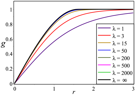
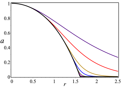
Figure 7: The profiles $g(r)$ (upper) and $a(r)$ (lower) coming from generalized Maxwell-Chern-Simons-Higgs model (V) with $G(g)=1$ and $\omega(g)=\lambda g^{2\lambda-2}$. Observe that $\lambda=1$ (indigo lines) represents the usual MCSH model and the true compacton solution is given by $\lambda=\infty$ (black lines).

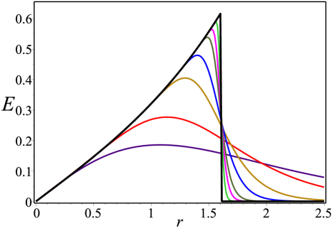
Figure 8: The scalar potential $A_{0}(r)$ (upper) and the electric field $E(r)$ (lower) coming from generalized Maxwell-Chern-Simons-Higgs model (V) with $G(g)=1$ and $\omega(g)=\lambda g^{2\lambda-2}$. Observe that $\lambda=1$ (indigo lines) represents the usual MCSH model and the true compacton solution is given by $\lambda=\infty$ (black lines).

The compacton boundary conditions satisfied by the profiles $g(r)$, $a(r)$ and $A_{0}(r)$ are

$$g(0) = 0,\;\;a(0)=n,\;\;A_{0}^{\prime}(0)=0,$$ (149)

$$g(r) = 1,\;\;a(r)=0,\;\;A_{0}(r)=0,\;\;r_{c}\leq r<\infty.\quad$$ (150)

The radial distance $r_{c}<\infty$ is the value where the profile $g(r)$ reaches the vacuum value, the gauge field profile $a(r)$ and scalar potential $A_{0}(r)$ becomes null.

The system is solved analytically to be

$$g^{(\infty)}(r) = \left(\frac{r}{r_{c}}\right)^{n}\exp\left[\frac{e^{2}v^{2}}{\kappa^{2}}\left(1-\frac{I(0,\kappa r)}{I(0,\kappa r_{c})}\right)\right]\Theta\left(r_{c}-r\right)$$ (151)

$$+\Theta\left(r-r_{c}\right),$$

$$a^{(\infty)}(r) = n\left(1-\frac{rI(1,\kappa r)}{r_{c}I(1,\kappa r_{c})}\right)\Theta\left(r_{c}-r\right),$$ (152)

$$A^{(\infty)}_{0}(r) = \frac{ev^{2}}{\kappa}\left(-1+\frac{I(0,\kappa r)}{I(0,\kappa r_{c})}\right)\Theta\left(r_{c}-r\right).$$ (153)

The radial distance $r_{c}$ is computed from the equation

$$I(0,\kappa r_{c})=r_{c}\frac{e^{2}v^{2}}{n\kappa}I(1,\kappa r_{c}),$$ (154)

where the function $I(\nu,x)$ is the modified Bessel function of the first kind and order $\nu$.

The magnetic field and BPS energy density of the Maxwell-Chern-Simons-Higgs compacton are

$$B^{(\infty)}(r) = ev^{2}\frac{I(0,\kappa r)}{I(0,\kappa r_{c})}\Theta(r_{c}-r),$$ (155)

$$\varepsilon_{{}_{BPS}}^{(\infty)}(r) = e^{2}v^{4}\left(\frac{I(0,\kappa r)}{I(0,\kappa r_{c})}\right)^{2}\Theta(r_{c}-r)$$

$$+e^{2}v^{4}\left(\frac{I(1,\kappa r)}{I(0,\kappa r_{c})}\right)^{2}\Theta(r_{c}-r).$$

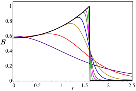
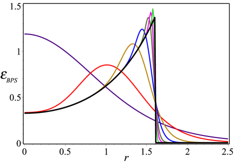
Figure 9: The magnetic field $B(r)$ (upper) and the BPS energy density $\varepsilon_{{}_{BPS}}(r)$ (lower) coming from generalized Maxwell-Chern-Simons-Higgs model (V) with $G(g)=1$ and $\omega(g)=\lambda g^{2\lambda-2}$. Observe that $\lambda=1$ (indigo lines) represents the usual MCSH model and the true compacton solution is given by $\lambda=\infty$ (black lines).

In order to compute the numerical solutions we choose the upper signs in equations (133) and (134), $e=1$, $v=1$, $\kappa=-1$ and winding number $n=1$. The profiles for the Higgs and gauge fields are given in Fig. 7, the correspondent ones for the scalar potential and for the electric field are depicted in Fig. 8. We can note again that an effective compact topological defect it is formed for large values of $\lambda$. This feature can be seen from the magnetic field and BPS energy density profiles in Fig. 9. Alike in the previous studied models the analytic MCSH compactons are formed for $\lambda=\infty$, they are represented by the solid black lines in Figs. 7, 8 and 9.

VI Remarks and conclusions

We have found self-dual or BPS configurations in Abelian-Higgs generalized models which given origin to new effective compact and true compacton configurations. Our goal was obtained by means of a consistent implementation of the BPS formalism which besides to provide the self-dual or BPS equations have also allowed to found the explicit form of the generalizing function $\omega(|\phi|)$ (see Eq. (16)) which is parameterized by the positive parameter $\lambda$. Such a parameter determine explicitly new families of self-dual potentials for every model and consequently characterize their self-dual configurations. We draw attention to the importance to obtain self-dual effective compact and analytic true compacton configurations in Abelian Higgs. This models enhance the space of self-dual solutions which probably will imply in interesting applications in physics and mathematics, for example, the construction of the respective supersymmetric extensions SUSY .

For every model we have studied the vortex solutions arising from the respective self-dual equations. The numerical analysis have shown that for sufficiently large values of $\lambda$ the profiles (of the Higgs field, gauge field, magnetic field, BPS energy density) are very alike with the ones of an effective compacton solution but still preserve a tail in their asymptotic decay. For every model, we have also analyzed the limit $\lambda\rightarrow\infty$ for arbitrary winding number $n$. Our analysis have shown that for $\lambda=\infty$ arises analytical compacton structures in all models (see black line profiles in all figures along the manuscript).

Finally, we are considering the interesting challenge of looking for effective compact structures in gauge field models which engender monopoles or skyrmions, for example. Advances in this direction will be reported elsewhere.

Competing Interests

The authors declare that there is no conflict of interests regarding the publication of this paper.

- (1) C. Armendariz-Picon, T. Damour and V. Mukhanov, Phys. Lett. B 458, 209 (1999).
- (2) C. Armendariz-Picon and E. A. Lim, J. Cosmol. Astropart. Phys. 08, 007 (2005).
- (3) V. Mukhanov and A. Vikman, J. Cosmol. Astropart. Phys. 02, 004 (2005).
- (4) A. Sen, JHEP 0207, 065 (2002).
- (5) N. Arkani-Hamed, H.-C. Cheng, M. A. Luty, S. Mukohyama, JHEP 0405, 074 (2004).
- (6) D. Bazeia, E. da Hora, C. dos Santos and R. Menezes, Phys. Rev. D 81, 125014 (2010); D. Bazeia, E. da Hora, R. Menezes, H. P. de Oliveira and C. dos Santos, Phys. Rev. D 81, 125016 (2010; C. dos Santos and E. da Hora, Eur. Phys. J. C 70, 1145 (2010); Eur. Phys. J. C 71, 1519 (2011); C. dos Santos, Phys. Rev. D 82, 125009 (2010); D. Bazeia, E. da Hora, C. dos Santos, R. Menezes, Eur. Phys. J. C 71, 1833 (2011); R. Casana, M.M. Ferreira, Jr., E. da Hora, Phys.Rev. D 86 085034 (2012).
- (7) E. Babichev, Phys. Rev. D 74, 085004 (2006); E. Babichev, Phys.Rev.D 77, 065021 (2008); C. Adam, J. Sanchez-Guillen and A. Wereszczynski, J. Phys. A 40, 13625 (2007); Erratum-ibid. A 42, 089801 (2009); C. Adam, N. Grandi, J. Sanchez-Guillen and A. Wereszczynski, J. Phys. A 41, 212004 (2008); Erratum- ibid. A 42, 159801 (2009); C. Adam, N. Grandi, P. Klimas, J. Sanchez-Guillen and A. Wereszczynski, J. Phys. A 41, 375401 (2008); C. Adam, P. Klimas, J. Sanchez-Guillen and A. Wereszczynski, J. Phys. A 42, 135401 (2009).
- (8) Rodolfo Casana,Lucas Sourrouille, Mod. Phys. Lett. A 29, 1450124 (2014); Lucas Sourrouille, Physical Review D 86, 085014 (2012).
- (9) E. Babichev, Phys. Rev. D 74, 085004 (2006); D. Bazeia, L. Losano, R. Menezes and J. C. R. E. Oliveira, Eur. Phys. J. C 51, 953 (2007).
- (10) C. Armendariz-Picon, T. Damour, V. Mukhanov, Phys. Lett. B 458, 209 (1999).
- (11) H. Nielsen and P. Olesen, Nucl. Phys. B 61, 1064 (1973).
- (12) P.-O. Jubert, R. Allenspach, and A. Bischof, Phys. Rev.B 69, 220410(R) (2004).
- (13) A. Fert, V. Cros, and J. Sampaio, Nature Nanotech. 8, 152 (2013).
- (14) N. Romming et al., Science 341, 636 (2013).
- (15) C. Adam, J. Sanchez-Guillen, A. Wereszczynski, Phys. Lett. B 691, 105 (2010).
- (16) Betti Hartmann, Burkhard Kleihaus, Jutta Kunzb, Isabell Schaffer, Phys. Lett. B 714, 120 (2012).
- (17) J. M. Speight, J. Phys. A: Math. Theor. 43, 405201 (2010).
- (18) C. Adam, T. Romanczukiewicz, J. Sanchez-Guillen and A. Wereszczynski, Phys. Rev. D 81, 085007 (2010).
- (19) E. B. Bogomol’nyi, Sov. J. Nuc. Phys. 24, 449 (1976); M. Prasad and C. Sommerfield, Phys. Rev. Lett. 35, 760 (1975).
- (20) R. Jackiw and E. J. Weinberg, Phys. Rev. Lett. 64, 2234 (1990). R. Jackiw, K. Lee and E. J. Weinberg, Phys. Rev. D 42, 3488 (1990).
- (21) C. Lee, K. Lee and H. Min, Phys. Lett. B 252, 79 (1990).
- (22) A. A. Belavin and A. M. Polyakov, JETP Lett. 22, 245 (1975).
- (23) R. Rajaraman, Solitons and Instantons (North-Holland, Amsterdam, 1982). W. J. Zakrzewski, Low Dimensional Sigma Models (Hilger, Bristol, 1989).
- (24) B. J. Schroers, Phys. Lett. B 356, 291 (1995); G. Nardelli, Phys. Rev. Lett. 73 2524 (1994); M. Arai, M. Naganuma, M. Nitta and N. Sakai, Nucl. Phys. B 652 35 (2003); J.M. Baptista, Commun. Math. Phys. 261 161 (2006); A. Alonso-Izquierdo, W. Garcia Fuertes and J. Mateos Guilarte, JHEP 02 139 (2015).
- (25) P. Mukherjee, Phys. Rev. D 58, 105025 (1998).
- (26) P. K. Ghosh and S. K. Ghosh, Phys. Lett. B 366, 199 (1996).
- (27) P. Mukherjee, Phys. Lett. B 403, 70 (1997).
- (28) K. Kimm, K. Lee and T. Lee, Phys. Rev. D 53, 4436 (1996).
- (29) J. Han, H.-S. Nam, Lett. Math. Phys. 73, 17 (2005).
- (30) D. Bazeia, E. da Hora, R. Menezes, H. P. de Oliveira, and C. dos Santos, Phys. Rev. D 81, 125016 (2010).
- (31) D. Bazeia, L. Losano, M. A. Marques, R. Menezes, I. Zafalan , Eur. Phys. J. C 77, 63 (2017).
- (32) D. Bazeia, E. da Hora, and D. Rubiera-Garcia, Phys. Rev. D 84, 125005 (2011).
- (33) Rodolfo Casana, Lucas Sourrouille, Adv. High Energy Phys. 2016, 5315649 (2016).
- (34) A. A. Abrikosov, Sov. Phys. JETP 5, 1174 (1957).
- (35) A. Vilenkin and E. P. S. Shellard, Cosmic Strings and Other Topological Defects (Cambridge University Press, Cambridge, England, 1994).
- (36) D. Bazeia, E. da Hora, C. dos Santos, and R. Menezes, Eur. Phys. J. C 71, 1833 (2011).
- (37) R. Casana, M. M. Ferreira, E. da Hora, and C. dos Santos, Adv. High Energy Phys. 2014, 210929 (2014).
- (38) B. Born and L. Infeld, Proc. Roy. Soc. A 144, 425 (1935); P. A. M. Dirac, Proc. Roy. Soc. A 268, 57 (1962).
- (39) G. Boillat, J. Math. Phys. 11, 941 (1970); G. W. Gibbons, Nucl. Phys. B 514, 603 (1998).
- (40) K. Shiraishi and S. Hirenzaki, Int. J. Mod. Phys. A 6, 2635 (1991).
- (41) R. Casana, E. da Hora, D. Rubiera-Garcia, and C. dos Santos, Eur. Phys. J. C 75, 380 (2015).
- (42) H. Vega and F. Schaposnik, Phys. Rev. D 14, 1100 (1976).
- (43) Zyun F. Ezawa, Quantum Hall Effects, second edition, World Scientific (2008).
- (44) R. Jackiw and S. Y. Pi, Prog. Theor. Phys. Suppl. 107, 1 (1992); Gerald V. Dunne, Lect.Notes Phys. M 36 (1995); Gerald V. Dunne, [arXiv:hep-th/9902115]; F. A. Schaposnik, [arXiv:hep-th/0611028]; Peter A. Horvathy and Pengming Zhang, Phys. Rept. 481, 83 (2009).
- (45) R. Jackiw and E. J. Weinberg, Physical Review Letters 64, 2234 (1990); Pac, Phys. Rev. Lett. 64 2230 (1990).
- (46) R. Jackiw and S. Y. Pi, Phys. Rev. Lett. 64, 2969 (1990); R. Jackiw and S. Y. Pi, Phys. Rev. D 42, 3500 (1990); Erratum-ibid. D 48, 3929 (1993).
- (47) R. Jackiw, Ki-Myeong Lee and E.J. Weinberg, Phys.Rev. D 42, 3488 (1990).
- (48) C. Lee, K. Lee and E.J. Weinberg, Phys. Lett. B 243, 105 (1990).
- (49) Paul and A. Khare, Phys. Lett. B 171, 244 (1986).
- (50) P.K. Ghosh, Phys. Rev. D 49, 5458 (1994)
- (51) D. Bazeia, R. Casana, E. da Hora, R. Menezes, Phys. Rev. D 85, 125028 (2012)
- (52) E. Witten and D. Olive, Phys. Lett. B 78, 97 (1978); Jose D. Edelstein, Carlos Nunez, Fidel Schaposnik, Phys. Lett. B 329, 39 (1994); W. Garcia Fuertes and J. Mateos Guilarte, J. Math. Phys. 38 6214 (1997); Y. Isozumi, M. Nitta, K. Ohashi and N. Sakai, Phys. Rev. D 71 065018 (2005).