Random Subspace with Trees for Feature Selection Under Memory Constraints

Abstract

Dealing with datasets of very high dimension is a major challenge in machine learning. In this paper, we consider the problem of feature selection in applications where the memory is not large enough to contain all features. In this setting, we propose a novel tree-based feature selection approach that builds a sequence of randomized trees on small subsamples of variables mixing both variables already identified as relevant by previous models and variables randomly selected among the other variables. As our main contribution, we provide an in-depth theoretical analysis of this method in infinite sample setting. In particular, we study its soundness with respect to common definitions of feature relevance and its convergence speed under various variable dependance scenarios. We also provide some preliminary empirical results highlighting the potential of the approach.

1 Motivation

We consider supervised learning and more specifically feature selection in applications where the memory is not large enough to contain all data. Such memory constraints can be due either to the large volume of available training data or to physical limits of the system on which training is performed (eg., mobile devices). A straightforward, but often efficient, way to handle such memory constraint is to build and average an ensemble of models, each trained on only a random subset of samples and/or features that can fit into memory. Such simple ensemble approaches have the advantage to be applicable to any batch learning algorithm, considered as a black-box, and they have been shown empirically to be very effective in terms of predictive performance, in particular when combined with trees, and even when samples and/or features are selected uniformly at random [see, eg., 1, 2]. In particular, and independently of any considerations about memory constraints, feature subsampling has been shown in several works to be a very effective way to introduce randomization when building ensembles of models [3, 4]. The idea of feature subsampling has also been investigated in the context of feature selection, where several authors have proposed to repeatedly apply a multivariate feature selection technique on random subsets of features and then to aggregate the results obtained on these subsets [see, eg., 5, 6, 7, 8, 9].

In this work, focusing on feature subsampling, we adopt a simplistic setting where we assume that only q input features (among $p$ in total, with typically $q\ll p$) can fit into memory. In this setting, we study ensembles of randomized decision trees trained each on a random subset of $q$ features. In particular, we are interested in the properties of variable importance scores derived from these models and their exploitation to perform feature selection. In contrast to a purely uniform sampling of the features, we propose in Section 3 a modified sequential random subspace (SRS) approach that biases the random selection of the features at each iteration towards features already found relevant by previous models. As our main contribution, we perform in Section 4 an in-depth theoretical analysis of this method in infinite sample size condition. In particular, we show that (1) this algorithm provides some interesting asymptotic guarantees to find all (strongly) relevant variables, (2) that accumulating previously found variables can reduce the number of trees needed to find relevant variables by several orders of magnitudes with respect to the standard random subspace method in some scenarios, and (3) that these scenarios are relevant for a large class of (PC) distributions. As an important additional contribution, our analysis also sheds some new light on both the popular random subspace and random forests methods that are special cases of the SRS algorithm. Finally, Section 5 presents some preliminary empirical results with the approach on several artificial and real datasets.

2 Feature selection and tree-based methods

This section gives the necessary background about feature selection and random forests.

2.1 Feature relevance and feature selection

Let us denote by $V$ the set of inputs variables, with $|V|=p$, and by $Y$ the output. Feature selection is concerned about the identification in $V$ of the (most) relevant variables. A common definition of relevance is as follows [10]:

Definition 1.

A variable $X\in V$ is relevant iff there exists a subset $B\subset V$ such that $X\mathbin{\mathchoice{\hbox to0.0pt{\hbox{\set@color$\displaystyle\perp$}\hss}\kern 3.46875pt{\not}\kern 3.46875pt\hbox{\set@color$\displaystyle\perp$}}{\hbox to0.0pt{\hbox{\set@color$\textstyle\perp$}\hss}\kern 3.46875pt{\not}\kern 3.46875pt\hbox{\set@color$\textstyle\perp$}}{\hbox to0.0pt{\hbox{\set@color$\scriptstyle\perp$}\hss}\kern 2.36812pt{\not}\kern 2.36812pt\hbox{\set@color$\scriptstyle\perp$}}{\hbox to0.0pt{\hbox{\set@color$\scriptscriptstyle\perp$}\hss}\kern 1.63437pt{\not}\kern 1.63437pt\hbox{\set@color$\scriptscriptstyle\perp$}}}Y|B$. A variable is irrelevant if it is not relevant.

Relevant variables can be further divided into two categories [10]:

Definition 2.

A variable $X$ is strongly relevant iff $Y\mathbin{\mathchoice{\hbox to0.0pt{\hbox{\set@color$\displaystyle\perp$}\hss}\kern 3.46875pt{\not}\kern 3.46875pt\hbox{\set@color$\displaystyle\perp$}}{\hbox to0.0pt{\hbox{\set@color$\textstyle\perp$}\hss}\kern 3.46875pt{\not}\kern 3.46875pt\hbox{\set@color$\textstyle\perp$}}{\hbox to0.0pt{\hbox{\set@color$\scriptstyle\perp$}\hss}\kern 2.36812pt{\not}\kern 2.36812pt\hbox{\set@color$\scriptstyle\perp$}}{\hbox to0.0pt{\hbox{\set@color$\scriptscriptstyle\perp$}\hss}\kern 1.63437pt{\not}\kern 1.63437pt\hbox{\set@color$\scriptscriptstyle\perp$}}}X|V\setminus\{X\}$. A variable $X$ is weakly relevant if it is relevant but not strongly relevant.

Strongly relevant variables are thus those variables that convey information about the output that no other variable (or combination of variables) in $V$ conveys.

The problem of feature selection usually can take two flavors [11]:

• All-relevant problem: finding all relevant features.

• Minimal optimal problem: finding a subset $M\subseteq V$ such that $Y\mathbin{\mathchoice{\hbox to0.0pt{\hbox{\set@color$\displaystyle\perp$}\hss}\kern 3.46875pt{}\kern 3.46875pt\hbox{\set@color$\displaystyle\perp$}}{\hbox to0.0pt{\hbox{\set@color$\textstyle\perp$}\hss}\kern 3.46875pt{}\kern 3.46875pt\hbox{\set@color$\textstyle\perp$}}{\hbox to0.0pt{\hbox{\set@color$\scriptstyle\perp$}\hss}\kern 2.36812pt{}\kern 2.36812pt\hbox{\set@color$\scriptstyle\perp$}}{\hbox to0.0pt{\hbox{\set@color$\scriptscriptstyle\perp$}\hss}\kern 1.63437pt{}\kern 1.63437pt\hbox{\set@color$\scriptscriptstyle\perp$}}}V\setminus M|M$ and such that no proper subset of $M$ satisfies this property. A subset $M$ solution to the minimal optimal problem is called a Markov boundary (of $Y$ with respect to $V$).

A Markov boundary always contains all strongly relevant variables and potentially some weakly relevant ones. In general, the minimal optimal problem does not have a unique solution. For strictly positive distributions however, the Markov boundary $M$ of $Y$ is unique and a feature $X$ belongs to $M$ iff $X$ is strongly relevant [11]. In this case, the solution to the minimal optimal problem is thus the set of all strongly relevant variables.

In what follows, we will need to qualify relevant variables according to their degree:

Definition 3.

The degree of a relevant variable $X$, denoted $deg(X)$, is defined as the minimal size of a subset $B\subseteq V$ such that $Y\mathbin{\mathchoice{\hbox to0.0pt{\hbox{\set@color$\displaystyle\perp$}\hss}\kern 3.46875pt{\not}\kern 3.46875pt\hbox{\set@color$\displaystyle\perp$}}{\hbox to0.0pt{\hbox{\set@color$\textstyle\perp$}\hss}\kern 3.46875pt{\not}\kern 3.46875pt\hbox{\set@color$\textstyle\perp$}}{\hbox to0.0pt{\hbox{\set@color$\scriptstyle\perp$}\hss}\kern 2.36812pt{\not}\kern 2.36812pt\hbox{\set@color$\scriptstyle\perp$}}{\hbox to0.0pt{\hbox{\set@color$\scriptscriptstyle\perp$}\hss}\kern 1.63437pt{\not}\kern 1.63437pt\hbox{\set@color$\scriptscriptstyle\perp$}}}X|B$.

Relevant variables $X$ of degree 0, i.e. such that $Y\mathbin{\mathchoice{\hbox to0.0pt{\hbox{\set@color$\displaystyle\perp$}\hss}\kern 3.46875pt{\not}\kern 3.46875pt\hbox{\set@color$\displaystyle\perp$}}{\hbox to0.0pt{\hbox{\set@color$\textstyle\perp$}\hss}\kern 3.46875pt{\not}\kern 3.46875pt\hbox{\set@color$\textstyle\perp$}}{\hbox to0.0pt{\hbox{\set@color$\scriptstyle\perp$}\hss}\kern 2.36812pt{\not}\kern 2.36812pt\hbox{\set@color$\scriptstyle\perp$}}{\hbox to0.0pt{\hbox{\set@color$\scriptscriptstyle\perp$}\hss}\kern 1.63437pt{\not}\kern 1.63437pt\hbox{\set@color$\scriptscriptstyle\perp$}}}X$ unconditionally, will be called marginally relevant.

We will say that a subset $B$ such that $Y\mathbin{\mathchoice{\hbox to0.0pt{\hbox{\set@color$\displaystyle\perp$}\hss}\kern 3.46875pt{\not}\kern 3.46875pt\hbox{\set@color$\displaystyle\perp$}}{\hbox to0.0pt{\hbox{\set@color$\textstyle\perp$}\hss}\kern 3.46875pt{\not}\kern 3.46875pt\hbox{\set@color$\textstyle\perp$}}{\hbox to0.0pt{\hbox{\set@color$\scriptstyle\perp$}\hss}\kern 2.36812pt{\not}\kern 2.36812pt\hbox{\set@color$\scriptstyle\perp$}}{\hbox to0.0pt{\hbox{\set@color$\scriptscriptstyle\perp$}\hss}\kern 1.63437pt{\not}\kern 1.63437pt\hbox{\set@color$\scriptscriptstyle\perp$}}}X|B$ is minimal if there is no proper subset $B^{\prime}\subseteq B$ such that $Y\mathbin{\mathchoice{\hbox to0.0pt{\hbox{\set@color$\displaystyle\perp$}\hss}\kern 3.46875pt{\not}\kern 3.46875pt\hbox{\set@color$\displaystyle\perp$}}{\hbox to0.0pt{\hbox{\set@color$\textstyle\perp$}\hss}\kern 3.46875pt{\not}\kern 3.46875pt\hbox{\set@color$\textstyle\perp$}}{\hbox to0.0pt{\hbox{\set@color$\scriptstyle\perp$}\hss}\kern 2.36812pt{\not}\kern 2.36812pt\hbox{\set@color$\scriptstyle\perp$}}{\hbox to0.0pt{\hbox{\set@color$\scriptscriptstyle\perp$}\hss}\kern 1.63437pt{\not}\kern 1.63437pt\hbox{\set@color$\scriptscriptstyle\perp$}}}X|B^{\prime}$. The following two propositions give a characterization of these minimal subsets.

Proposition 1.

A minimal subset $B$ such that $Y\mathbin{\mathchoice{\hbox to0.0pt{\hbox{\set@color$\displaystyle\perp$}\hss}\kern 3.46875pt{\not}\kern 3.46875pt\hbox{\set@color$\displaystyle\perp$}}{\hbox to0.0pt{\hbox{\set@color$\textstyle\perp$}\hss}\kern 3.46875pt{\not}\kern 3.46875pt\hbox{\set@color$\textstyle\perp$}}{\hbox to0.0pt{\hbox{\set@color$\scriptstyle\perp$}\hss}\kern 2.36812pt{\not}\kern 2.36812pt\hbox{\set@color$\scriptstyle\perp$}}{\hbox to0.0pt{\hbox{\set@color$\scriptscriptstyle\perp$}\hss}\kern 1.63437pt{\not}\kern 1.63437pt\hbox{\set@color$\scriptscriptstyle\perp$}}}X|B$ for a relevant variable $X$ contains only relevant variables.  (Proof in Appendix LABEL:app:only-relevant)

Proposition 2.

Let $B$ denote a minimal subset such that $Y\mathbin{\mathchoice{\hbox to0.0pt{\hbox{\set@color$\displaystyle\perp$}\hss}\kern 3.46875pt{\not}\kern 3.46875pt\hbox{\set@color$\displaystyle\perp$}}{\hbox to0.0pt{\hbox{\set@color$\textstyle\perp$}\hss}\kern 3.46875pt{\not}\kern 3.46875pt\hbox{\set@color$\textstyle\perp$}}{\hbox to0.0pt{\hbox{\set@color$\scriptstyle\perp$}\hss}\kern 2.36812pt{\not}\kern 2.36812pt\hbox{\set@color$\scriptstyle\perp$}}{\hbox to0.0pt{\hbox{\set@color$\scriptscriptstyle\perp$}\hss}\kern 1.63437pt{\not}\kern 1.63437pt\hbox{\set@color$\scriptscriptstyle\perp$}}}X|B$ for a relevant variable $X$. For all $X^{\prime}\in B$, $deg(X^{\prime})\leq|B|$.  (Proof in Appendix LABEL:app:only-degree)

These two propositions show that a minimal conditioning $B$ that makes a variable dependent on the output is composed of only relevant variables whose degrees are all smaller or equal to the size of $B$. We will provide in Section 4.2 a more stringent characterization of variables in minimum conditionings in the case of a specific class of distributions.

2.2 Tree-based methods and variable importances

A decision tree [12] represents an input-ouput model with a tree structure, where each interior node is labeled with a test based on some input variable and each leaf node is labeled with a value of the output. The tree is typically grown using a recursive procedure which identifies at each node $t$ the split $s$ that maximizes the mean decrease of some node impurity measure (e.g., Shannon entropy in classification and variance in regression).

Typically, decision trees suffer from a high variance that can be very efficiently reduced by building instead an ensemble of randomized trees and aggregating their predictions. Several techniques have been proposed in the literature to grow randomized trees. For example, bagging [13] builds each tree with the classical algorithm from a bootstrap sample from the original learning sample. Ho [3]’s random subspace method grows each tree from a subset of the features of size $K\leq p$ randomly drawn from $V$. Breiman [14]’s Random Forests algorithm combines bagging with a local random selection of $K(\leq p)$ variables at each node from which to identify the best split.

Given an ensemble of trees, several methods have been proposed to evaluate the importance of the variables for predicting the output [12, 14]. We will focus here on one particular measure called the mean decrease impurity (MDI) importance for which some theoretical characterization has been proposed in [15]. This measure adds up the weighted impurity decreases over all nodes $t$ in a tree $T$ where the variable $X$ to score is used to split and then averaging this quantity over all trees in the ensemble, i.e.:

$$Imp(X)=\frac{1}{N_{T}}\sum_{T}\sum_{t\in T:v(s_{t})=X}p(t)\Delta i(s_{t},t),\mbox{ with }\Delta i(s_{t},t)=i(t)-p(t_{L})i(t_{L})-p(t_{R})i(t_{R})$$ (1)

where $i$ is the impurity measure, $p(t)$ is the proportion of samples reaching node $t$, $v(s_{t})$ is the variable used in the split $s_{t}$ at node $t$, and $t_{L}$ and $t_{R}$ are the left and right successors of $t$ after the split.

Louppe et al. [15] derived several interesting properties of this measure under the assumption that all variables are discrete and that splits on these variables are multi-way (i.e., each potential value of the splitting variable is associated with one successor of the node to split). In particular, they obtained the following result in asymptotic sample and ensemble size conditions:

Theorem 1.

$X\in V$ is irrelevant to $Y$ with respect to $V$ if and only if its infinite sample importance as computed with an infinite ensemble of fully developed totally randomized trees built on $V$ for $Y$ is 0 (Theorem 3 in Louppe et al. [15]).

Totally randomized trees are trees obtained by setting Random Forests randomization parameter $K$ to 1. This result shows that MDI importance derived from trees grown with $K=1$ is asymptotically consistent with the definition of variable relevance given in the previous section. In Section 4.1, we will actually extend this result to values of $K$ greater than 1.

3 Sequential random subspace

Algorithm 1 Sequential Random Subspace algorithm

Inputs:
Data: $Y$ the output and $V$, the set of all input variables (of size $p$).
Algorithm: $q$, the subspace size, and $T$ the number of iterations, $\alpha\in[0,1]$, the percentage of memory devoted to previously found features.
Tree: $K$, the tree randomization parameter
Output: An ensemble of $T$ trees and a subset $F$ of features
Algorithm:

1. $F=\emptyset$

2. Repeat $T$ times:

   1. Let $Q=R\cup C$, with $R$ a subset of $\min\{\lfloor\alpha q\rfloor,|F|\}$ features randomly picked in $F$ without replacement and $C$ a subset of $q-|R|$ features randomly selected in $V\setminus R$.

   2. Build a decision tree $\cal T$ from $Q$ using randomization parameter $K$.

   3. Add to $F$ all features from $Q$ that get an importance greater than zero in $\cal T$.

In this paper, we consider a simplistic memory-constrained setting where it is assumed that only $q$ input features can fit into memory at once, with typically $q$ small with respect to $p$. Under this hypothesis, Algorithm 1 describes the proposed sequential random subspace (SRS) algorithm to build an ensemble of randomized trees, which generalizes the Random Subspace (RS) method [3]. The idea of this method is to bias the random selection of the features at each iteration towards features that have already been found relevant by the previous trees. A parameter $\alpha$ is introduced that controls the degree of accumulation of previously identified features. When $\alpha=0$, SRS reduces to the standard RS method. When $\alpha=1$, all previously found features are kept while when $\alpha<1$, some room in memory is left for randomly picked features, which ensures some permanent exploration of the feature space. Further randomization is introduced in the tree building step through the parameter $K\in[1,q]$, ie. the number of variables sampled at each tree node for splitting. Variable importance is assumed to be the MDI importance. This algorithm returns both an ensemble of trees and a subset $F$ of variables, those that get an importance (significantly) greater than 0 in at least one tree of the ensemble. Importance scores for the variables can furthermore be derived from the final ensemble using (1). In what follows, we will denote by $F^{K,\alpha}_{q,T}$ and $Imp^{K,\alpha}_{q,T}(X)$ resp. the set of features and the importance of feature $X$ obtained from an ensemble grown with SRS with parameters $K$, $\alpha$, $q$ and $T$.

The modification of the RS algorithm is actually motivated by Propositions 1 and 2, stating that the relevance of high degree features can be determined only when they are analysed jointly with other relevant features of equal or lower degree. From this result, one can thus expect that accumulating previously found features will fasten the discovery of higher degree features on which they depend through some snowball effect. In the next section, we provide a theoretical asymptotic analysis of the SRS method that confirms and quantifies this effect.

Note that the SRS method can also be motivated from the perspective of accuracy. When $q\ll p$ and the number of relevant features $r$ is also much smaller than the total number of features $p$ ($r\ll p$), many trees with standard RS are grown from subsets of features that contain only very few, if any, relevant features and are thus expected not to be better than random guessing [4]. In such setting, RS ensembles are thus expected not to be very accurate.

Example 1.

With $p=10000$, $r=10$ and $q=50$, the proportion of trees in a RS ensemble grown from only irrelevant variables is $C^{q}_{p-r}/C^{q}_{p}=0.95$.

With SRS (and $\alpha>0$), we ensure that more and more relevant variables are given to the tree growing algorithm as iterations proceed and therefore we reduce the chance to include totally useless trees in the ensemble. Note however that in finite settings, there is a potential risk of overfitting when accumulating the variables. The parameter $\alpha$ thus controls a new bias-variance tradeoff and should be tuned appropriately. We will study the impact of SRS on accuracy empirically in Section 5.

4 Theoretical analysis

In this section, we carry out a theoretical analysis of the proposed method when seen as a feature selection technique. This analysis is performed in asymptotic sample size condition and assuming that all features are discrete. We proceed in two steps. First, we study the soundness of the algorithm, ie., its capacity to retrieve the relevant variables when the number of trees is infinite. Second, we study its convergence properties, ie. the number of trees needed to retrieve all relevant variables in different scenarios.

4.1 Soundness

Our goal in this section is to characterize the sets of features $F^{K,\alpha}_{q,\infty}$ that are identified by the SRS algorithm, depending on the value of its parameters $q$, $\alpha$, and $K$, in an asymptotic setting, ie. assuming an infinite sample size and an infinite forest ($T=\infty$). Note that in asymptotic setting, a variable is relevant as soon as its importance in one of the tree is strictly greater than zero and we thus have the following equivalence for all variables $X\in V$:

$$X\in F^{K,\alpha}_{q,\infty}\Leftrightarrow Imp^{K,\alpha}_{q,\infty}(X)>0$$

Furthermore, in infinite sample size setting, irrelevant variables always get a zero importance and thus, whatever the parameters, we have the following property for all $X\in V$:

$$X\mbox{ irrelevant}\Rightarrow X\notin F^{K,\alpha}_{q,\infty}\mbox{ (and }Imp^{K,\alpha}_{q,\infty}(X)=0\mbox{)}.$$

The method parameters thus only affect the number and nature of the relevant variables that can be found. Denoting by $r$ ($\leq p$) the number of relevant variables, we will analyse separately the case $r\leq q$ (all relevant variables can fit into memory) and the case $r>q$ (all relevant variables can not fit into memory).

All relevant variables can fit into memory ($r\leq q$).

Let us first consider the case of the RS method ($\alpha=0$). In this case, Louppe et al. [15] have shown the following asymptotic formula for the importances computed with totally randomized trees ($K=1$):

$$Imp_{q,\infty}^{1,0}(X)=\sum_{k=0}^{q-1}\dfrac{1}{C_{p}^{k}}\sum_{B\in{\cal P}_{k}(V^{-m})}I(X;Y|B),$$ (2)

where ${\cal P}_{k}(V^{-m})$ is the set of subsets of $V^{-m}=V\setminus\{x_{m}\}$ of cardinality $k$. Given that all terms are positive, this sum will be strictly greater than zero if and only if there exists a subset $B\subseteq V$ of size at most $q-1$ such that $Y\mathbin{\mathchoice{\hbox to0.0pt{\hbox{\set@color$\displaystyle\perp$}\hss}\kern 3.46875pt{\not}\kern 3.46875pt\hbox{\set@color$\displaystyle\perp$}}{\hbox to0.0pt{\hbox{\set@color$\textstyle\perp$}\hss}\kern 3.46875pt{\not}\kern 3.46875pt\hbox{\set@color$\textstyle\perp$}}{\hbox to0.0pt{\hbox{\set@color$\scriptstyle\perp$}\hss}\kern 2.36812pt{\not}\kern 2.36812pt\hbox{\set@color$\scriptstyle\perp$}}{\hbox to0.0pt{\hbox{\set@color$\scriptscriptstyle\perp$}\hss}\kern 1.63437pt{\not}\kern 1.63437pt\hbox{\set@color$\scriptscriptstyle\perp$}}}X|B$, or equivalently if $deg(X)<q$. When $\alpha=0$, RS with $K=1$ will thus find all and only the relevant variables of degree at most $q-1$. Given Proposition 1, the degree of a variable $X$ can not be larger than $r-1$ and thus as soon as $r\leq q$, we have the guarantee that RS with $K=1$ will find all and only the relevant variables. Actually, this result remains valid when $\alpha>0$. Indeed, asymptotically, only relevant variables will be selected in the $F$ subset by SRS and given that all relevant variables can fit into memory, cumulating them will not impact the ability of SRS to explore all conditioning subsets $B$ composed of relevant variables. We thus have the following result:

Proposition 3.

$\forall\alpha$, if $r\leq q$:  $X\in F_{q,\infty}^{1,\alpha}\mbox{ iff }X\mbox{ is relevant}.$

In the case of non-totally randomized trees ($K>1$), we lose the guarantee to find all relevant variables even when $r\leq q$. Indeed, there is potentially a masking effect due to $K>1$ that might prevent the conditioning needed for a given variable to be relevant to appear in a tree branch. However, we have the following general result:

Theorem 2.

$\forall\alpha,K$, if $r\leq q$: $X\mbox{ strongly relevant}\Rightarrow X\in F_{q,\infty}^{K,\alpha}$  (Proof in Appendix LABEL:app:stronglyrelpruned)

There is thus no masking effect possible for the strongly relevant features when $K>1$ as soon as the number of relevant features is lower than $q$. For a given $K$, the features found by SRS will thus include all strongly relevant variables and some (when $K>1$) or all (when $K=1$) weakly relevant ones. It is easy to show that increasing $K$ can only decrease the number of weakly relevant variables found. Using $K=1$ will thus provide a solution for the all-relevant problem, while increasing $K$ will provide a better and better approximation of the minimal-optimal problem in the case of strictly positive distributions (see Section 2.1).

Interestingly, Theorem 2 remains true when $q=p$, ie., when forests are grown without any feature sampling. It thus extends Theorem 1 from [15] for arbitrary $K$ in the case of standard random forests.

All relevant variables can not fit into memory ($r>q$).

When all relevant variables can not fit into memory, we do not have the guarantee anymore to explore all minimal conditionings required to find all (strongly or not) relevant variables, whatever the values of $K$ and $\alpha$. When $\alpha=0$, we have the guarantee however to identify the relevant variables of degree strictly lower than $q$. When $\alpha>1$, some space in memory will be devoted to previously found variables that will introduce some further masking effect. We nevertheless have the following general results (without proof):

Proposition 4.

$\forall X:$  $X\mbox{ relevant and }deg(X)<(1-\alpha)q\Rightarrow X\in F^{1,\alpha}_{q,\infty}.$

Proposition 5.

$\forall K,X:$  $X\mbox{ strongly relevant and }deg(X)<(1-\alpha)q\Rightarrow X\in F^{K,\alpha}_{q,\infty}.$

In these propositions, $(1-\alpha)q$ is simply the amount of memory that always remains available for the exploration of variables not yet found relevant.

Discussion.

Results in this section show that SRS is a sound approach for feature selection as soon as either the memory is large enough to contain all relevant variables or the degree of the relevant variables is not too high. In this latter case, the approach will be able to detect all strongly relevant variables whatever its parameters ($K$ and $\alpha$) and the total number of features $p$. Of course, these parameters will have a potentially strong influence on the number of trees needed to reach convergence (see the next section) and the performance in finite setting.

4.2 Convergence

Results in the previous section show that accumulating relevant variables has no impact on the capacity at finding relevant variables asymptotically (when $r\leq q$). It has however a potentially strong impact on the convergence speed of the algorithm, as measured for example by the expected number of trees needed to find all relevant variables. Indeed, when $\alpha=0$ and $q\ll p$, the number of iterations/trees needed to find relevant variables of high degree can be huge as finding them requires to sample them together with all features in their conditioning. Given Proposition 2, we know that a minimum subset $B$ such that $X\mathbin{\mathchoice{\hbox to0.0pt{\hbox{\set@color$\displaystyle\perp$}\hss}\kern 3.46875pt{\not}\kern 3.46875pt\hbox{\set@color$\displaystyle\perp$}}{\hbox to0.0pt{\hbox{\set@color$\textstyle\perp$}\hss}\kern 3.46875pt{\not}\kern 3.46875pt\hbox{\set@color$\textstyle\perp$}}{\hbox to0.0pt{\hbox{\set@color$\scriptstyle\perp$}\hss}\kern 2.36812pt{\not}\kern 2.36812pt\hbox{\set@color$\scriptstyle\perp$}}{\hbox to0.0pt{\hbox{\set@color$\scriptscriptstyle\perp$}\hss}\kern 1.63437pt{\not}\kern 1.63437pt\hbox{\set@color$\scriptscriptstyle\perp$}}}Y|B$ for a relevant variable $X$ contains only relevant variables. This suggests that accumulating previously found relevant features can improve significantly the convergence, as each time one relevant variable is found it increases the chance to find a relevant variable of higher degree that depends on it. In what follows, we will quantify the effect of accumulation on convergence speed in different best-case and worst-case scenarios and under some simplifications of the tree building procedure. We will conclude by a theorem highlighting the interest of the SRS method in the general class of PC distributions.

Scenarios and assumptions.

The convergence speed is in general very much dependent on the data distribution. We will study here the following three specific scenarios (where features $\{X_{1},\ldots,X_{r}\}$ are the only relevant features):

• Chaining: The only and minimal conditioning that makes variable $X_{i}$ relevant is $\{X_{1},\ldots,X_{i-1}\}$ (for $i=1,\ldots,r$). We thus have $deg(X_{i})=i-1$. This scenario should correspond to the most favorable situation for the SRS algorithm.

• Clique: The only and minimal conditioning that makes variable $X_{i}$ relevant is $\{X_{1},\ldots,X_{i-1},X_{i+1},\ldots,X_{r}\}$ (for $i=1,\ldots,r$). We thus have $deg(X_{i})=r-1$ for all $i$. This is a rather defavorable case for both RS and SRS since finding a relevant variable implies to draw all of them at the same iteration.

• Marginal-only: All variables are marginally relevant. We will furthermore make the assumption that these variables are all strongly relevant. They can not be masked mutually. This scenario is the most defavorable case for SRS (versus RS) since accumulating relevant variables is totally useless to find the other relevant variables and it should actually slow down the convergence as it will reduce the amount of memory left for exploration.

In Appendix LABEL:sec:avgtime, we provide explicit formulation of the expected number of iterations needed to find all $r$ relevant features in the chaining and clique scenarios both when $\alpha=0$ (RS) and $\alpha=1$ (SRS). In Appendix LABEL:sec:mc, we provide order 1 Markov chains that model the evolution through the iterations of the number of variables found in the three scenarios when $\alpha=0$ and $\alpha=1$. These chains can be used to compute numerically the expected number of relevant variables found through the iterations (and in the case of the marginal-only setting, the expected number of iterations to find all variables). These derivations are obtained assuming $r\leq q$, $K=q$, and under additional simplifying assumptions detailed in Appendix LABEL:app:assumption-convergence.

Results and discussion.

Tables 1a, 1b, and 1c show the expected number of iterations needed to find all relevant variables for various configurations of the parameters $p$, $q$, and $r$, in the three scenarios. Figure 1 plots the expected number of variables found at each iteration both for RS and SRS in the three scenarios for some particular values of the parameters.

Table 1: Expected number of iterations needed to find all relevant variables for various configurations of parameters $p$, $q$ and $r$ with RS ($\alpha=0$) and SRS ($\alpha=1$) in the three scenarios.

Config (p,q,r)	RS	SRS
$10^{4},100,1$	100	100
$10^{4},100,2$	10100	200
$10^{4},100,3$	$>10^{6}$	301
$10^{4},100,5$	$>10^{10}$	506
$10^{5},100,3$	$>10^{9}$	3028

(a) Chaining.

Config (p,q,r)	RS	SRS
$10^{4},100,1$	100	100
$10^{4},100,2$	30300	10302
$10^{4},100,3$	$5\cdot 10^{6}$	$10^{6}$
$10^{4},100,4$	$9\cdot 10^{8}$	$10^{8}$
$10^{4},10^{3},4$	$83785$	$11635$

(b) Clique.

Config (p,q,r)	RS	SRS
$10^{4},100,10$	291	312
$10^{4},100,50$	448	757
$10^{4},100,90$	506	2797
$10^{4},100,100$	1123	16187
$25000,100,50$	1123	1900

(c) Marginal-only.

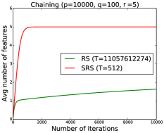
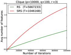
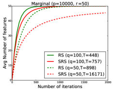
Figure 1: Evolution of the number of selected features in the different scenarios.

From these results, we can draw several conclusions. In all cases, expected times (ie., number of iterations/trees to find all relevant variables) depend mostly on the ratio $\frac{q}{p}$, not on absolute values of $q$ and $p$. The larger this ratio, the faster the convergence. Parameter $r$ has a strong impact on convergence speed in all three scenarios.

The most impressive improvements with SRS are obtained in the chaining hypothesis, where convergence is improved by several orders of magnitude (Table 1a and Figure 1a) . At fixed $p$ and $q$, the time needed by RS indeed grows exponentially with $r$ ($\simeq(\frac{p}{q})^{r}$ if $r\ll q$), while time grows linearly with $r$ for the SRS method ($\simeq r\frac{p}{q}$ if $r\ll q$) (see Eq. (LABEL:ref:naive) and (LABEL:ref:smart) in Appendix LABEL:sec:avgtime).

In the case of cliques, both RS and SRS need many iterations to find all features from the clique (see Table 1b and Figure 1b). SRS goes faster than RS but the improvement is not as important as in the chaining scenario. This can be explained by the fact that SRS can only improve the speed when the first feature of the clique has been found. Since the number of iterations needed to find the $r$ features from the clique for RS is close to $r$ times the number of iterations needed to find one feature from the clique, SRS can only decrease at best the number of iterations by approximately a factor $r$ (see Eq. (LABEL:eqn:naiveclique) and (LABEL:eqn:smartclique) in Appendix LABEL:sec:avgtime).

In the marginal-only setting, SRS is actually slower than RS because the only effect of cumulating the variables is to leave less space in memory for exploration. The decrease of computing times is however contained when $r$ is not too close to $q$ (see Table 1c and Figure 1c).

Since we can obtain very significant improvement in the case of the chaining and clique scenarios and we only increase moderately the number of iterations in the marginal-only scenario (when $r$ is not too close from $q$), we can reasonably expect improvement in general settings that mix these scenarios.

PC distributions and chaining.

Chaining is the most interesting scenario in terms of convergence improvement through variable accumulation. In this scenario, SRS makes it possible to find high degree relevant variables with a reasonable amount of trees, when finding these variables would be mostly untractable for RS. We provide below two theorems that show the practical relevance of this scenario in the specific case of PC distributions.

A PC distribution is defined as a strictly positive (P) distribution that satisfies the composition (C) property stated as follows [11]:

Property 1.

For any disjoint sets of variables $R,S,T,U\subseteq V\cup\{Y\}$:

$$S\mathbin{\mathchoice{\hbox to0.0pt{\hbox{\set@color$\displaystyle\perp$}\hss}\kern 3.46875pt{}\kern 3.46875pt\hbox{\set@color$\displaystyle\perp$}}{\hbox to0.0pt{\hbox{\set@color$\textstyle\perp$}\hss}\kern 3.46875pt{}\kern 3.46875pt\hbox{\set@color$\textstyle\perp$}}{\hbox to0.0pt{\hbox{\set@color$\scriptstyle\perp$}\hss}\kern 2.36812pt{}\kern 2.36812pt\hbox{\set@color$\scriptstyle\perp$}}{\hbox to0.0pt{\hbox{\set@color$\scriptscriptstyle\perp$}\hss}\kern 1.63437pt{}\kern 1.63437pt\hbox{\set@color$\scriptscriptstyle\perp$}}}T|R\mbox{ and }S\mathbin{\mathchoice{\hbox to0.0pt{\hbox{\set@color$\displaystyle\perp$}\hss}\kern 3.46875pt{}\kern 3.46875pt\hbox{\set@color$\displaystyle\perp$}}{\hbox to0.0pt{\hbox{\set@color$\textstyle\perp$}\hss}\kern 3.46875pt{}\kern 3.46875pt\hbox{\set@color$\textstyle\perp$}}{\hbox to0.0pt{\hbox{\set@color$\scriptstyle\perp$}\hss}\kern 2.36812pt{}\kern 2.36812pt\hbox{\set@color$\scriptstyle\perp$}}{\hbox to0.0pt{\hbox{\set@color$\scriptscriptstyle\perp$}\hss}\kern 1.63437pt{}\kern 1.63437pt\hbox{\set@color$\scriptscriptstyle\perp$}}}U|R\Rightarrow S\mathbin{\mathchoice{\hbox to0.0pt{\hbox{\set@color$\displaystyle\perp$}\hss}\kern 3.46875pt{}\kern 3.46875pt\hbox{\set@color$\displaystyle\perp$}}{\hbox to0.0pt{\hbox{\set@color$\textstyle\perp$}\hss}\kern 3.46875pt{}\kern 3.46875pt\hbox{\set@color$\textstyle\perp$}}{\hbox to0.0pt{\hbox{\set@color$\scriptstyle\perp$}\hss}\kern 2.36812pt{}\kern 2.36812pt\hbox{\set@color$\scriptstyle\perp$}}{\hbox to0.0pt{\hbox{\set@color$\scriptscriptstyle\perp$}\hss}\kern 1.63437pt{}\kern 1.63437pt\hbox{\set@color$\scriptscriptstyle\perp$}}}T\cup U|R$$

The composition property prevents the occurence of cliques and is preserved under marginalization. PC actually represents a rather large class of distributions that encompasses for example jointly Gaussian distributions and DAG-faithful distributions [11].

The composition property allows to make Proposition 2 more stringent in the case of PC:

Proposition 6.

Let $B$ denote a minimal subset $B$ such that $Y\mathbin{\mathchoice{\hbox to0.0pt{\hbox{\set@color$\displaystyle\perp$}\hss}\kern 3.46875pt{\not}\kern 3.46875pt\hbox{\set@color$\displaystyle\perp$}}{\hbox to0.0pt{\hbox{\set@color$\textstyle\perp$}\hss}\kern 3.46875pt{\not}\kern 3.46875pt\hbox{\set@color$\textstyle\perp$}}{\hbox to0.0pt{\hbox{\set@color$\scriptstyle\perp$}\hss}\kern 2.36812pt{\not}\kern 2.36812pt\hbox{\set@color$\scriptstyle\perp$}}{\hbox to0.0pt{\hbox{\set@color$\scriptscriptstyle\perp$}\hss}\kern 1.63437pt{\not}\kern 1.63437pt\hbox{\set@color$\scriptscriptstyle\perp$}}}X|B$ for a relevant variable $X$. If the distribution $P$ over $V\cup\{Y\}$ is PC, then for all $X^{\prime}\in B$, $deg(X^{\prime})<|B|$.  (Proof in Appendix LABEL:app:only-degree-pc)

In addition, one has the following result:

Theorem 3.

For any PC distribution, let us assume that there exists a non empty minimal subset $B=\{X_{1},\ldots,X_{k}\}\subset V\setminus\{X\}$ of size $k$ such that $X\mathbin{\mathchoice{\hbox to0.0pt{\hbox{\set@color$\displaystyle\perp$}\hss}\kern 3.46875pt{\not}\kern 3.46875pt\hbox{\set@color$\displaystyle\perp$}}{\hbox to0.0pt{\hbox{\set@color$\textstyle\perp$}\hss}\kern 3.46875pt{\not}\kern 3.46875pt\hbox{\set@color$\textstyle\perp$}}{\hbox to0.0pt{\hbox{\set@color$\scriptstyle\perp$}\hss}\kern 2.36812pt{\not}\kern 2.36812pt\hbox{\set@color$\scriptstyle\perp$}}{\hbox to0.0pt{\hbox{\set@color$\scriptscriptstyle\perp$}\hss}\kern 1.63437pt{\not}\kern 1.63437pt\hbox{\set@color$\scriptscriptstyle\perp$}}}Y|B$ for a relevant variable $X$. Then, variables $X_{1}$ to $X_{k}$ can be ordered into a sequence $\{X^{\prime}_{1},\ldots,X^{\prime}_{k}\}$ such that $deg(X^{\prime}_{i})<i$ for all $i=1,\ldots,k$.  (Proof in Appendix LABEL:app:pcchain)

This theorem shows that, when the data distribution is PC, for all relevant variables of degree $k$, the $k$ variables in its minimal conditioning form a chain of variables of increasing degrees (at worst). For such distribution, we thus have the guarantee that SRS find all relevant variables with a number of iterations that grows almost only linearly with the maximum degree of relevant variables (see Eq.LABEL:ref:smart in Appendix LABEL:sec:avgtime), while RS would be unable to find relevant variables of even small degree.

5 Experiments

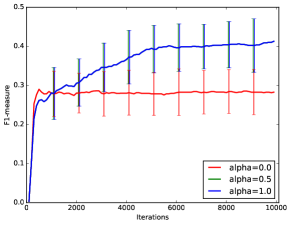
(a) SRS with $q=0.05\times p$ on a dataset with $p=50000$ features and $r=20$ relevant features.

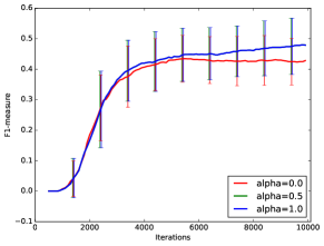
(b) SRS with $q=0.005\times p$ on a dataset with $p=50000$ features and $r=20$ relevant features.

Figure 2: Evolution of the evaluation of the feature subset found by RS and SRS using the F1-measure computed with respect to relevant features. A higher value means that more relevant features have been found. This experiment was computed on an artificial dataset (similar to madelon) of 50000 features with 20 relevant features and for two sizes of memory.

Although our main contribution is the theoretical analysis in asymptotic setting of the previous section, we present here a few preliminary experiments in finite setting as a first illustration of the potential of the method.One of the main difficulties to implement the SRS algorithm as presented in Algorithm 1 is step 2(c) that decides which variable should be incorporated in $F$ at each iteration. In infinite sample size setting, a variable with a non-zero importance in a single tree is guaranteed to be truly relevant. Mutual informations estimated from finite samples however will always be greater than 0 even for irrelevant variables. One should thus replace step 2(c) by some statistical significance tests to avoid the accumulation of irrelevant variables that would jeopardize the convergence of the algorithm. In our experiments here, we use a random probe (ie., an artificially created irrelevant variable) to derive a statistical measure assessing the relevance of a variable [16]. Details about this test are given in Appendix LABEL:app:results.

Figure 2 evaluates the feature selection ability of SRS for three values of $\alpha$ (including $\alpha=0$) and two memory sizes (250 and 2500) on an artificial dataset with 50000 features, among which only 20 are relevant (see Appendix LABEL:app:results for more details). The two plots show the evolution of the F1-score comparing the selected features (in $F$) with the truly relevant ones as a function of the number of iterations. As expected, SRS ($\alpha>0$) is able to find better feature subsets than RS ($\alpha=0$) for both memory sizes and both values of $\alpha>0$.

Additional results are provided in Appendix LABEL:app:results that compare the accuracy of ensembles grown with SRS for different values of $\alpha$ and on 13 classification problems. These comparisons clearly show that accumulating the relevant variables is beneficial most of the time (eg., SRS with $\alpha=0.5$ is significantly better than RS on 7 datasets, comparable on 5, and significantly worse on only 1). Interestingly, SRS ensembles with $\alpha=0.5$ are also most of the time significantly better than ensembles of trees grown without memory constraint (see Appendix LABEL:app:results for more details).

6 Conclusions and future work

Our main contribution is a theoretical analysis of the SRS (and RS) methods in infinite sample setting. This analysis showed that both methods provide some guarantees to identify all relevant (or all strongly) relevant variables as soon as the number of relevant variables or their degree is not too high with respect to the memory size. Compared to RS, SRS can reduce very strongly the number of iterations needed to find high degree variables in particular in the case of PC distributions. We believe that our results shed some new light on random subspace methods for feature selection in general as well as on tree-based methods, which should help designing better feature selection procedures.

Although some preliminary experiments were provided that support the theoretical analysis, more work is clearly needed to evaluate the approach empirically on controlled and real high-dimensional problems. We believe that the statistical test used to decide which feature to include in the relevant set should be improved with respect to our first implementation based on the introduction of a random probe. One drawback of the SRS method with respect to RS is that it can not be parallelized anymore because of its sequential nature. It would be interesting to design and study variants of the method that are allowed to grow parallel ensembles at each iteration instead of single trees. Finally, relaxing the main hypotheses of our theoretical analysis would be also of course of great interest.

See pages - of sutera17-supp.pdf

References

- Chawla et al. [2004] Nitesh V. Chawla, Lawrence O. Hall, Kevin W. Bowyer, and W. Philip Kegelmeyer. Learning ensembles from bites: A scalable and accurate approach. J. Mach. Learn. Res., 5:421–451, December 2004. ISSN 1532-4435.
- Louppe and Geurts [2012] Gilles Louppe and Pierre Geurts. Ensembles on random patches. In Machine Learning and Knowledge Discovery in Databases, pages 346–361. Springer, 2012.
- Ho [1998] Tin Kam Ho. The random subspace method for constructing decision forests. Pattern Analysis and Machine Intelligence, IEEE Transactions on, 20(8):832–844, 1998.
- Kuncheva et al. [2010] Ludmila I Kuncheva, Juan J Rodríguez, Catrin O Plumpton, David EJ Linden, and Stephen J Johnston. Random subspace ensembles for fmri classification. Medical Imaging, IEEE Transactions on, 29(2):531–542, 2010.
- Dramiński et al. [2008] Michał Dramiński, Alvaro Rada-Iglesias, Stefan Enroth, Claes Wadelius, Jacek Koronacki, and Jan Komorowski. Monte carlo feature selection for supervised classification. Bioinformatics, 24(1):110–117, 2008.
- Lai et al. [2006] Carmen Lai, Marcel JT Reinders, and Lodewyk Wessels. Random subspace method for multivariate feature selection. Pattern recognition letters, 27(10):1067–1076, 2006.
- Konukoglu and Ganz [2014] Ender Konukoglu and Melanie Ganz. Approximate false positive rate control in selection frequency for random forest. arXiv preprint arXiv:1410.2838, 2014.
- Nguyen et al. [2015] Thanh-Tung Nguyen, He Zhao, Joshua Zhexue Huang, Thuy Thi Nguyen, and Mark Junjie Li. A new feature sampling method in random forests for predicting high-dimensional data. In Advances in Knowledge Discovery and Data Mining, pages 459–470. Springer, 2015.
- Dramiński et al. [2016] Michał Dramiński, Michał J Dabrowski, Klev Diamanti, Jacek Koronacki, and Jan Komorowski. Discovering networks of interdependent features in high-dimensional problems. In Big Data Analysis: New Algorithms for a New Society, pages 285–304. Springer, 2016.
- Kohavi and John [1997] Ron Kohavi and George H John. Wrappers for feature subset selection. Artificial intelligence, 97(1):273–324, 1997.
- Nilsson et al. [2007] Roland Nilsson, José M Peña, Johan Björkegren, and Jesper Tegnér. Consistent feature selection for pattern recognition in polynomial time. The Journal of Machine Learning Research, 8:589–612, 2007.
- Breiman et al. [1984] L. Breiman, J. H. Friedman, R. A. Olshen, and C. J. Stone. Classification and regression trees. 1984.
- Breiman [1996] Leo Breiman. Bagging predictors. Machine learning, 24(2):123–140, 1996.
- Breiman [2001] Leo Breiman. Random forests. Machine learning, 45(1):5–32, 2001.
- Louppe et al. [2013] G. Louppe, L. Wehenkel, A. Sutera, and P. Geurts. Understanding variable importances in forests of randomized trees. In Advances in neural information processing, 2013.
- Stoppiglia et al. [2003] H. Stoppiglia, G. Dreyfus, R. Dubois, and Y. Oussar. Ranking a random feature for variable and feature selection. Journal of Machine Learning Research, 3:1399–1414, 2003.