Factor Models with Real Data:
a Robust Estimation of the Number of Factors

Abstract

Factor models are a very efficient way to describe high dimensional vectors of data in terms of a small number of common relevant factors. This problem, which is of fundamental importance in many disciplines, is usually reformulated in mathematical terms as follows. We are given the covariance matrix $\Sigma$ of the available data. $\Sigma$ must be additively decomposed as the sum of two positive semidefinite matrices $D$ and $L$: $D$ — that accounts for the idiosyncratic noise affecting the knowledge of each component of the available vector of data — must be diagonal and $L$ must have the smallest possible rank in order to describe the available data in terms of the smallest possible number of independent factors.

In practice, however, the matrix $\Sigma$ is never known and therefore it must be estimated from the data so that only an approximation of $\Sigma$ is actually available. This paper discusses the issues that arise from this uncertainty and provides a strategy to deal with the problem of robustly estimating the number of factors.

I Introduction

Describing a large amount of data by means of a small number of factors carrying most of the information is an important problem in modern data analysis with applications ranging in all fields of science. One of the classical methods for this purpose is to resort to factor models that were first developed at the beginning of the last century by Spearman [spearman_1904] in the framework of the so-called mental tests as an attempt at “the procedure of eliciting verifiable facts” in determining psychical tendencies from the tests results. From this first seed a rich stream of literature was developed at the interface between psychology and mathematics with the main focus on the case of a single common factor underlying the available data: necessary and sufficient conditions for the data to be compatible with a single common factor were derived in [BURT_1909, Spearman-Holzinger-24], see also [Bekker-deLeeuw_1987] and references therein for a detailed historical reconstruction of the derivation of these conditions. The interest for this kind of model has grown rapidly also outside the psychology community and analysis of factor models, or factor analysis has become an important tool in statistics, econometrics, systems theory and many engineering fields [KALMAN_SELECTION_ECONOMETRICS_1983, SCHUPPEN_1986, Bekker-deLeeuw_1987, PICCI_1987, GEWEKE_DYNAMIC, PICCI_PINZONI_1986, Pena_BOX__1987, ON_THE_PENA_BOX_MODEL_2001, deistler2007, DEISTLER_1997, ANDERSON_DEISTLER_1993, SARGENT_SIM_1977, forni_lippi_2001, ENGLE_ONE_FACTOR_1981, WATSON_ALGORITHMS_1983], [mclachlan1997wiley]; see also the more recent papers [Bottegal-Picci, MFA, DEISTLER_2015, fan2013large], [bertsimas2017certifiably, delgado2014rank] where many other references are listed. A detailed geometric description of this problem is presented in [scherrer1998structure]. In the seminal paper [anderson1956statistical] a maximum likelihood approach in a statistical testing framework is proposed.

In the original formulation the construction of a factor model is equivalent to the mathematical problem of additively decomposing a given positive definite matrix $\Sigma$ — modeling the covariance of the data — as

$$\Sigma=L+D$$ (1)

where both $L$ and $D$ are positive semidefinite, and $D$ — modeling the covariance of the idiosyncratic noise — is diagonal. The rank of $L$ is the number of (latent or hidden) common factors that explain the available data. One of the key aspects of factor analysis is to determine the minimum number of latent factors or, equivalently, a decomposition (1) where the rank of $L$ is minimal. This is therefore a particular case of a matrix additive decomposition problem that arises naturally in numerous frameworks and have therefore received a great deal of attention, see [Chandrasekaran-Sanghavi-Parrilo-Willsky, agarwal2012noisy, LATENTG, BSL] and references therein. We hasten to remark that the problem of minimizing the rank of $L$ in the decomposition (1) is extremely hard so that, the convex relaxation is usually considered where, in place of the rank, the nuclear norm (i.e. the trace) of $L$ is minimized. This is a very good approximation that most often returns, with reasonable computational burden, a solution $L$ with minimum rank.

In [THURSTONE_1935],[Kelley_1928],[Ledermann_1937] an upper bound $r(n)$ — known as Ledermann bound — was proposed for the minimal rank $r_{m}(\Sigma)$ of $L$ in terms if the dimension $n$ of the matrix $\Sigma$:

$$r_{m}(\Sigma)\leq r(n):=\Big{\lfloor}\frac{2n+1-\sqrt{8n+1}}{2}\Big{\rfloor}.$$

This bound, however, is based on heuristics that have never been proven rigorously; a pétale de rose is the prize for a positive demonstration of this fact [Hakim1976]. Interestingly, almost half a century later in [RANK_REDUCIBILITY_1982] a related result was established: the set of matrices $\Sigma$ for which $r_{m}(\Sigma)<r(n)$ has zero Lebesgue measure. As a consequence of this result we have the following observation that may be regarded as the basic premise of our effort. When $n$ is large the Ledermann bound $r(n)$ is not much smaller than $n$. Therefore, even if our data do come from a factor model with a small number $r$ of latent factors, only a set of zero measure of $\hat{\Sigma}$ in a neighbourhood of $\Sigma$ can be decomposed in such a way that the corresponding $L$ matrix in its decomposition (1) has rank $r$. Thus, unless we know $\Sigma$ with absolute precision, we cannot rely only on the decomposition (1) to recover such $r$. An example of this phenomenon is illustrated in Figure 1.

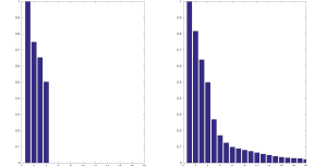
Figure 1: First $20$ singular values of the matrices $L$ (on the left) and $\hat{L}$ (on the right) obtained by applying the minimum trace factor analysis decomposition algorithm to a “true” covariance matrix $\Sigma\in\mathbb{R}^{40\times 40}$ of a model with $r=4$ latent factors and to an estimate $\hat{\Sigma}$ of $\Sigma$ obtained by generating $N=1000$ independent samples from a normal distribution $\mathcal{N}(0,\Sigma)$ and computing the corresponding sample covariance, respectively. Notice that the recovered matrix $L$ using as input the true $\Sigma$ is, up to negligible numerical errors, equal to the true low rank matrix.

The problem of estimating $r$ from an estimate $\hat{\Sigma}$ of $\Sigma$ is therefore of crucial importance and has been addressed in [bai2002determining] and [lam2012factor] by means of statistical methods. A similar issue has been addressed also in [ning2015linear] in the framework of the robustness of Frisch scheme. Here, we propose an alternative optimization-based approach which is based only on the estimate $\hat{\Sigma}$ and takes into account the uncertainty of this estimate. Hence, even if we can start from $N$ $n$-dimensional vectors (observations) the data of our problem are just the sample covariance $\hat{\Sigma}$ of these vectors and their number $N$. These two quantities summarize all the relevant information for our method in which we compute the matrix $\Sigma$ in such a way that the trace of $L$ in its additive decomposition (1) is minimized under a constraint limiting the Kullback-Leibler divergence between $\Sigma$ and $\hat{\Sigma}$ to a prescribed tolerance that depends on the precision of our estimate $\hat{\Sigma}$ and hence may be reliably chosen on the basis of the data numerosity $N$.

The proposed problem is analyzed by resorting to duality theory. The dual analysis is delicate to carry over, but yields a problem whose solution can be efficiently computed by employing an alternating direction method of multipliers (ADMM) algorithm. Moreover, the dual problem provides a necessary and sufficient condition for the uniqueness of the solution of the original problem.

The paper is organized as follows. In the Section II we recall the classical approach to factor analysis and, from it, we derive the formulation of our factor analysis problem. In Section III we describe how to establish, for a desired tolerance, an upper bound on the aforementioned Kullback-Leibler divergence. In Section IV we derive a dual formulation of our problem. In Section V we prove existence and uniqueness of the solution for the dual problem. Then, in Section LABEL:sec_recovery we show how to recover the solution of the primal problem. In Section LABEL:algorithm we present the numerical algorithm for solving the dual problem, while in Section LABEL:simulations the results of numerical simulations and an application to a real world example are presented. Finally, some conclusions are provided. The less instructive proofs that are essentially based on calculations are deferred to the Appendix.

Some of the results of this paper have been presented in preliminary form and mostly without proof in our conference paper [NF_CDC].

Notation: Given a vector space $\cal V$ and a subspace ${\cal W}\subset{\cal V}$, we denote by ${\cal W}^{\bot}$ the orthogonal complement of ${\cal W}$ in ${\cal V}$. Given a matrix $M$, we denote its transpose by $M^{\top}$; if $M$ is a square matrix $\operatorname{tr}(M)$ denotes its trace, i.e. the sum of the elements in the main diagonal of $M$; moreover, $|M|$ denotes the determinant of $M$ and $\sigma(M)$ denotes the spectrum of $M$, i.e. the set of its eigenvalues. We denote the spectral norm of $M$ as $\|M\|_{2}$. We endow the space of square real matrices with the following inner product: for $A,B\in{\mathbb{R}}^{n\times n}$, $\langle A,B\rangle:=\operatorname{tr}(A^{T}B)$. The kernel of a matrix (or of a linear operator) is denoted by $\ker(\cdot)$. The symbol $\mathbf{Q}_{n}$ denotes the vector space of real symmetric matrices of size $n$. If $X\in\mathbf{Q}_{n}$ is positive definite or positive semi-definite we write $X\succ 0$ or $X\succeq 0$, respectively. Moreover, we denote by $\mathbf{D}_{n}$ the vector space of diagonal matrices of size $n$; $\mathbf{D}_{n}$ is clearly a subspace of $\mathbf{Q}_{n}$ and we denote by $\mathbf{M}_{n}:=\mathbf{D}_{n}^{\bot}$ the orthogonal complement of $\mathbf{D}_{n}$ in $\mathbf{Q}_{n}$ (with respect to the inner product just defined). It is easy to see that $\mathbf{M}_{n}$ is the vector space of symmetric matrices of size $n$ having all the elements on the main diagonal equal to zero. We denote by $\operatorname{diag}(\cdot)$ both the operator mapping $n$ real elements $d_{i},i=1,...,n$ into the diagonal matrix having the $d_{i}$’s as elements in its main diagonal and the operator mapping a matrix $M\in\mathbb{R}^{n\times n}$ into an $n$-dimensional vector containing the diagonal elements of $M$. Then $\operatorname{diag}\operatorname{diag}(\cdot)$, that we denote by $\operatorname{diag^{2}}(\cdot)$, is the (orthogonal projection) operator mapping a square matrix $M$ into a diagonal matrix of the same size having the same main diagonal of $M$. We denote by $\operatorname{ofd}(\cdot)$ the self-adjoint operator orthogonally projecting $\mathbf{Q}_{n}$ onto $\mathbf{M}_{n}$, i.e. if $M\in\mathbf{Q}_{n}$, $\operatorname{ofd}(M)$ is the matrix of $\mathbf{M}_{n}$ in which each off-diagonal element is equal to the corresponding element of $M$ (and each diagonal element is clearly zero). Finally, we denote by $\otimes$ the Kronecker product between two matrices and by vec(X) the vectorization of a matrix X formed by stacking the columns of X into a single column vector.

II Problem Formulation

We consider a standard factor model in its static linear formulation

$$y =Ax+z$$ (2)

where $A\in\mathbb{R}^{n\times r}$, with $r<<n$, is the factor loading matrix, $x$ represents the (independent) latent factors and $z$ is the idiosyncratic component. $x$ and $z$ are independent Gaussian random vectors with zero mean and covariance matrix equal to the identity matrix of dimension $r$ and $D\in\mathbf{D}_{n}$, respectively. Note that, $Ax$ represents the latent variable. Consequently, $y$ is a Gaussian random vector with zero mean; we denote by $\Sigma$ its covariance matrix. Since $x$ and $z$ are independent we get that $\Sigma$ may be additively decomposed as in (1), where $L:=AA^{\top}$ and $D$ are the covariance matrices of $Ax$ and $z$, respectively. Thus, $L$ has rank equal to $r$, and $D$ is diagonal.

The objective of factor analysis consists in finding the most parsimonious “low-rank plus diagonal” decomposition of $\Sigma$, that is a decomposition (1) for which the rank of $L$ is minimal. This amounts to solve the minimum rank problem

$$\min_{L,D\in\mathbf{Q}_{n}} \text{ rank}(L)$$ (3)

subject to $$L,D\succeq 0$$

$$D\in\mathbf{D}_{n}$$

$${\Sigma}=L+D$$

which is, however, a hard problem. A well-known and widely used heuristic is the convex relaxation of (3), i.e. the trace minimization problem

$$\min_{L,D\in\mathbf{Q}_{n}} \text{ tr}(L)$$ (4)

subject to $$L,D\succeq 0$$

$$D\in\mathbf{D}_{n}$$

$${\Sigma}=L+D.$$

The substitution of the rank with the trace is justified by the fact that $\operatorname{tr}(L)$, i.e. the nuclear norm of $L$, is the convex hull of $\text{ rank}(L)$ over the set ${\cal S}:=\{L\in\mathbf{Q}_{n}\;\mathrm{s.t.}\;\|L\|_{2}\leq 1\}$, [FAZEL_MIN_RANK_APPLICATIONS_2002]. The relation between Problem (3) and Problem (4) has been first studied in [MIN_RANK_SHAPIRO_1982] and while these two problems are, in general, not equivalent, very often they have the same solution.

In practice, however, matrix $\Sigma$ is not known and needs to be estimated from a $N$-length realization (i.e. a data record) $\mathrm{y}_{1}\ldots\mathrm{y}_{N}$ of $y$. The typical choice is to take the sample covariance estimate

$$\hat{\Sigma}:=\frac{1}{N}\sum_{k=1}^{N}\mathrm{y}_{k}\mathrm{y}_{k}^{\top}$$ (5)

which is statistically consistent, i.e. the corresponding estimator almost surely converges to $\Sigma$ as $N$ tends to infinity. As discussed in the Introduction, by replacing $\Sigma$ with $\hat{\Sigma}$ the solution, in terms of minimum rank, will rapidly degrade. Indeed a delicate problem in factor analysis is the one of estimating the number of factors. Such a problem has been addressed by several important contributions, see the seminal works of Bai and Ng [bai2002determining] and of Lam and Yao [lam2012factor] and the references therein. Our objective is to address the same problem from a different perspective. In fact, we propose an optimization problem whose solution provides an estimate of the minimum number of factors by introducing an appropriate model for the error in the estimation of $\Sigma$. This model is based on an auxiliary Gaussian random vector $\hat{y}$ with zero mean and covariance matrix $\hat{\Sigma}$ that is regarded as a “model approximation” for $y$. To account for the estimation uncertainty, we assume that the distribution of $y$ (that is completely specified by its covariance matrix and hence is referred to by $\Sigma$) belongs to a “ball” centred in $\hat{y}$

$${\cal B}:=\{\Sigma\in\mathbf{Q}_{n}\;\mathrm{s.t.}\;\Sigma\succ 0,\;{\cal D}_{KL}(\Sigma\|\hat{\Sigma})\leq\delta/2\}$$ (6)

which is formed by placing a bound (i.e. tolerance) on the Kullback-Leibler divergence between $y$ and $\hat{y}$:

$${\cal D}_{KL}(\Sigma\|\hat{\Sigma}):=\frac{1}{2}\left(-\log|\Sigma|+\log|\hat{\Sigma}|+\operatorname{tr}(\Sigma\hat{\Sigma}^{-1})-n\right).$$

This way to deal with model uncertainty has been successfully applied in econometrics for model mispecification [ROBUSTNESS_HANSENSARGENT_2008] and in robust filtering [ROBUST_FILTERING, ROBUST_KALMAN_2017, LEVY_NIKOUKHAH_2004, ROBUST_CONV_2015, OPTIMALITY_ZORZI, convtau]. Accordingly, in order to estimate the minimum number of factors, we propose the following “robustification” of the minimum trace problem:

$$\min_{\Sigma,L,D\in\mathbf{Q}_{n}} \text{ tr}(L)$$ (7)

subject to $$L,D\succeq 0$$

$$D\in\mathbf{D}_{n}$$

$$\Sigma=L+D$$

$$\Sigma\in\cal B.$$

Note that, in (7) we can eliminate variable $D$, obtaining the equivalent problem

$$\min_{L,\Sigma\in\mathbf{Q}_{n}} \text{ tr}(L)$$ (8)

subject to $$L,\Sigma-L\succeq 0$$

$$\operatorname{ofd}(\Sigma-L)=0$$

$$\Sigma\succ 0$$

$$2\mathcal{D}_{KL}(\Sigma||\hat{\Sigma})\leq\delta.$$

It is worth noting that an alternative to Problem (8) is to consider $\mathcal{D}_{KL}(\Sigma||\hat{\Sigma})$ as a penalty term in the objective function rather than as a constraint. Such approach, however, would require a cross validation procedure to set the regularization parameter $\lambda$, i.e. we would have to solve an optimization problem for many values of $\lambda$. In contrast, the proposed problem is solved only once provided that $\delta$ is chosen in a suitable way, see the next section.

III The choice of $\delta$

The tolerance $\delta$ may be chosen by taking into account the accuracy of the estimate $\hat{\Sigma}$ of $\Sigma$ which, in turn, depends on the numerosity of the available data. This can be done by choosing a probability $\alpha\in(0,1)$ and a neighborhood of “radius” $\delta_{\alpha}$ (in the Kullback-Leibler topology) centered in $\hat{\Sigma}$ containing the “true” $\Sigma$ with probability $\alpha$. The Kullback-Leibler divergence in (8) is a function of the estimated sample covariance and as such its accuracy depends crucially on the numerosity of the available data. To asses this accuracy we propose an approach that hinges on the following scale-invariance property of the Kullback-Leibler divergence.

Lemma III.1

Let $y_{i}\sim\mathcal{N}(0,\Sigma),\,i=1,...,N$ be i.i.d. random variables taking values in $\mathbb{R}^{n}$ and define the sample covariance estimator

$$\hat{{\mathbf{\Sigma}}}=\dfrac{1}{N}\sum_{i=1}^{N}y_{i}y_{i}^{T}.$$

The Kullback-Leibler divergence between $\Sigma$ and $\hat{{\mathbf{\Sigma}}}$ is a random variable whose distribution depends only of the number $N$ of random variables and on the dimension $n$ of each random variable.

Proof:

We have

$$\hat{{\mathbf{\Sigma}}}=\dfrac{1}{N}\sum_{i=1}^{N}y_{i}y_{i}^{T}=\dfrac{1}{N}\Sigma^{1/2}\sum_{i=1}^{N}\tilde{y}_{i}\tilde{y}_{i}^{T}\Sigma^{1/2}=\Sigma^{1/2}Q_{N}\Sigma^{1/2}$$

with $\tilde{y}_{i}=\Sigma^{-1/2}y_{i}\sim\mathcal{N}(0,I_{n})$ and $Q_{N}:=\dfrac{1}{N}\sum_{i=1}^{N}\tilde{y}_{i}\tilde{y}_{i}^{T},$ is a random matrix taking values in $\mathbf{Q}_{n}$. Notice that at this point $\tilde{y}$ are normalized Gaussian random vectors and hence do not depend on the data nor on $\Sigma$. Thus, $Q_{N}$ is a random matrix whose distribution only depends on $N$ and $n$ (see Section III-A for more details). Hence, the Kullback-Leibler divergence between $\Sigma$ and the sample covariance estimator is

$$d: =\mathcal{D}_{KL}(\Sigma\|\hat{{\mathbf{\Sigma}}})=\dfrac{1}{2}\big{(}\log(|\hat{{\mathbf{\Sigma}}}\Sigma^{-1}|)+\text{tr}(\Sigma\hat{{\mathbf{\Sigma}}}^{-1})-n\big{)}$$ (9)

$$=\dfrac{1}{2}\big{(}\log\left(|Q_{N}|\right)+\text{tr}(Q_{N}^{-1})-n\big{)}.$$

∎In view of this result we can easily approximate the distribution of the random variable $2d=2\mathcal{D}_{KL}(\Sigma\|\hat{{\mathbf{\Sigma}}})$ by a standard Monte Carlo method. In particular, we can reliably estimate with arbitrary precision the value of $\delta$ for which $Pr\big{(}2\mathcal{D}_{KL}(\Sigma||\hat{\Sigma})\leq\delta\big{)}=\alpha$. As an alternative to this empiric approach for determining $\delta_{\alpha}$, we can also resort to an analytic one as discussed below.

III-A Gaussian Orthogonal Ensemble

Let us focus on the random matrix $Q_{N}$ that we have defined as $Q_{N}:=\dfrac{1}{N}\sum_{i=1}^{N}\tilde{y}_{i}\tilde{y}_{i}^{T}$ where $\tilde{y}_{i}\in\mathbb{R}^{n},\,i=1,...,N$, are i.i.d. random variables distributed as $\mathcal{N}(0,I_{n})$. We now introduce a new matrix $\tilde{Q}_{N}:=\sqrt{N}(Q_{N}-I_{n})=\sqrt{N}\dfrac{1}{N}\sum_{i=1}^{N}C_{i}$, where $C_{i}:=\tilde{y}_{i}\tilde{y}_{i}^{T}-I$ are i.i.d. symmetric random matrices with zero mean. It is immediate to check that for each $i$: any two distinct elements $[C_{i}]_{h,j}$ and $[C_{i}]_{k,l}$ of $C_{i}$ are uncorrelated as long as they do not occupy symmetric positions, i.e. whenever $(h,j)\neq(l,k)$, and ${\rm Var}\left[[C_{i}]_{h,j}\right]=\begin{cases}1,&\text{if }h\neq j\\ 2,&\text{if }h=j\end{cases}$. By the multivariate Central Limit Theorem, we have that $\tilde{Q}_{N}$ converges in distribution to the random matrix

$$X=\left(\begin{array}[]{cccc}\sqrt{2}\xi_{1,1}&\cdots&\cdots&\xi_{1,n}\\ \vdots&\ddots&&\vdots\\ \vdots&&\ddots&\vdots\\ \xi_{1,n}&\cdots&\cdots&\sqrt{2}\xi_{n,n}\end{array}\right)\in\mathbf{Q}_{n},$$

where $\{\xi_{i,j}\}$ are i.i.d. Gaussian random variables with mean 0 and variance 1. The set of these matrices is known as the Gaussian Orthogonal Ensemble, see [anderson2010introduction]. It is well known that the joint distribution of the eigenvalues $\lambda_{1}(X)\leq...\leq\lambda_{n}(X)$ of such matrices takes the following form:

$$p(\lambda_{1},...,\lambda_{n})=\bar{C}_{n}|\Delta(\lambda)|\prod_{i=1}^{n}\mathrm{e}^{-\lambda_{i}^{2}/4}$$

where $\lambda:=(\lambda_{1},...,\lambda_{n})$, $|\Delta(\lambda)|$ is the Vandermonde determinant associated with $\lambda$, which is given by:

$$|\Delta(\lambda)|=\prod_{i<j}(\lambda_{j}-\lambda_{i})$$

and $\bar{C}_{n}$ is defined as:

$$\bar{C}_{n}=\left(\int_{-\infty}^{+\infty}...\int_{-\infty}^{+\infty}|\Delta(\lambda)|\prod_{i=1}^{n}\mathrm{e}^{-\lambda_{i}^{2}/4}d\lambda_{i}\right)^{-1}.$$

It is not difficult to see that (9) can be rewritten as:

$$d=d(\lambda_{1},...,\lambda_{n})=\sum_{i=1}^{n}\dfrac{1}{2}\left(\log\left(\dfrac{\lambda_{i}}{\sqrt{N}}+1\right)-\dfrac{\lambda_{i}}{\lambda_{i}+\sqrt{N}}\right)$$ (10)

where $\lambda_{i}\in\sigma(\tilde{Q}_{N})$. Then, for a desired $\alpha$, we are interested in finding $\delta_{\alpha}$ such that

$$Pr(2d\leq\delta_{\alpha})=\alpha.$$

Such a value for $\delta_{\alpha}$ is given by the cumulative distribution function $F(\cdot)$:

$$F(\delta_{\alpha}) =Pr(2d\leq\delta_{\alpha})$$ (11)

$$=\int_{I(\delta_{\alpha})}2d(\lambda_{1},...,\lambda_{n})p(\lambda_{1},...,\lambda_{n})d\lambda$$

where $p(\lambda_{1},...,\lambda_{n})$ denotes the joint probability density function of the eigenvalues $\lambda_{1},...,\lambda_{n}$ and $I(\delta_{\alpha}):=\{(\lambda_{1},...,\lambda_{n}):d(\lambda_{1},...,\lambda_{n})\leq\delta_{\alpha}/2\}$. Given $\alpha$ the integral in (11) can be solved numerically for $\delta_{\alpha}$.

III-B An upper bound for $\delta_{\alpha}$

If the chosen level $\alpha$ is too large with respect to the sample size $N$, the computed $\delta_{\alpha}$ become excessively large so that there are diagonal matrices $\Sigma_{D}$ such that $2\mathcal{D}_{KL}(\Sigma_{D}||\hat{\Sigma})\leq\delta_{\alpha}$. In this case Problem (8) admits the trivial solution $L=0$ and $D=\Sigma_{D}$. In order to rule out this trivial situation we need to require that the maximum value for $\delta$ in (8) is strictly less than a certain $\delta_{max}$ that can be determined as follows: since the trivial solution $L=0$ would imply a diagonal $\Sigma$, that is $\Sigma=\Sigma_{D}:=\text{diag}(d_{1},...,d_{n})>0$, $\delta_{max}$ can be determined by solving the following minimization problem

$$\delta_{max}:=\min_{\Sigma_{D}\in\mathbf{D}_{n}}2\mathcal{D}_{KL}(\Sigma_{D}\|\hat{\Sigma}).$$ (12)

The following Proposition, whose proof is in Appendix, shows how to solve this problem.

Proposition III.1

Let $\gamma_{i}$ denote the $i$-th element in the main diagonal of the inverse of the sample covariance $\hat{\Sigma}^{-1}$. Then, the optimal $\Sigma_{D}$ which solves the minimization problem in (12) is given by

$$\Sigma_{D}=\text{diag}(\gamma_{1}^{-1},...,\gamma_{n}^{-1}).$$

Moreover, $\delta_{max}$ can be determined as

$$\delta_{max}=2\mathcal{D}_{KL}(\Sigma_{D}\|\hat{\Sigma})=\log|\operatorname{diag^{2}}(\hat{\Sigma}^{-1})\hat{\Sigma}|.$$ (13)

In what follows, we always assume that $\delta$ in (8) strictly less than $\delta_{max}$, so that the trivial solution $L=0$ is ruled out.

IV Dual Problem

By duality theory, we reformulate the constrained minimization problem in (8) as an unconstrained minimization problem. The associated Lagrangian is

$$\mathcal{L}(L, \Sigma,\lambda,\Lambda,\Gamma,\Theta)$$ (14)

$$= \text{tr}(L)+\lambda(-\log|\Sigma|+\log|\hat{\Sigma}|-n+\text{tr}(\hat{\Sigma}^{-1}\Sigma)-\delta)$$

$$-\text{tr}(\Lambda L)-\text{tr}(\Gamma(\Sigma-L))+\text{tr}{(\Theta\operatorname{ofd}(\Sigma-L)})$$

$$= \text{tr}(L)+\lambda(-\log|\Sigma|+\log|\hat{\Sigma}|-n+\text{tr}(\hat{\Sigma}^{-1}\Sigma)-\delta)$$

$$-\text{tr}(\Lambda L)-\text{tr}(\Gamma(\Sigma-L))+\text{tr}{(\operatorname{ofd}^{*}(\Theta)(\Sigma-L)})$$

$$= \text{tr}(L)+\lambda(-\log|\Sigma|+\log|\hat{\Sigma}|-n+\text{tr}(\hat{\Sigma}^{-1}\Sigma)-\delta)$$

$$-\text{tr}(\Lambda L)-\text{tr}(\Gamma(\Sigma-L))+\text{tr}{(\operatorname{ofd}(\Theta)(\Sigma-L)})$$

with $\lambda\in\mathbb{R},\lambda\geq 0$, and $\Lambda,\Gamma,\Theta\in\mathbf{Q}_{n}$ with $\Lambda,\Gamma\succeq 0$. In the last equality, we exploited the fact that the operator $\operatorname{ofd}(\cdot)$ is self-adjoint. Note that the Lagrangian (14) does not include the constraint $\Sigma\succ 0$: as we will see this condition is automatically met by the solution of the dual problem.
Notice also that in (14) we can recognize the fit term $2\lambda\mathcal{D}(\Sigma\|\hat{\Sigma})=\lambda(-\log|\Sigma|+\log|\hat{\Sigma}|-n+\text{tr}(\hat{\Sigma}^{-1}\Sigma))$ and the term $\text{tr}((I-\Lambda)L+(\operatorname{ofd}(\Theta)-\Gamma)(\Sigma-L))$ accounting for the complexity in the class of models (1) which induces low-rank on matrix $L$. Thus (14) can be interpreted as an alternative to the likelihood function with a complexity term.

The dual function is defined as the infimum of $\mathcal{L}(L,\Sigma,\lambda,\Lambda,\Gamma,\Theta)$ over $L$ and $\Sigma$.
Thanks to the convexity of the Lagrangian, we rely on standard variational methods to characterize the minimum.
The first variation of the Lagrangian (14) at $\Sigma$ in direction $\delta\Sigma\in\mathbf{Q}_{n}$ is

$$\delta\mathcal{L}(\Sigma;\delta\Sigma)=\text{tr}(-\lambda\Sigma^{-1}\delta\Sigma+\lambda\hat{\Sigma}^{-1}\delta\Sigma-\Gamma\delta\Sigma+\operatorname{ofd}(\Theta)\delta\Sigma).$$

We impose the optimality condition

$$\delta\mathcal{L}(\Sigma;\delta\Sigma)=0,\qquad\forall\delta\Sigma\in\mathbf{Q}_{n},$$

which is equivalent to require $\text{tr}(-\lambda\Sigma^{-1}\delta\Sigma+\lambda\hat{\Sigma}^{-1}\delta\Sigma-\Gamma\delta\Sigma+\operatorname{ofd}(\Theta)\delta\Sigma)=0$ for all $\delta\Sigma\in\mathbf{Q}_{n}$, obtaining

$$\Sigma=\lambda(\lambda\hat{\Sigma}^{-1}-\Gamma+\operatorname{ofd}(\Theta))$$ ^-1 (15)

provided that $\lambda\hat{\Sigma}^{-1}-\Gamma+\operatorname{ofd}(\Theta)\succ 0$ and $\lambda>0$, which is clearly equivalent to require that the optimal $\Sigma$ that minimizes the Lagrangian satisfies the constraint $\Sigma\succ 0$.

The first variation of the Lagrangian (14) at $L$ in direction $\delta L\in\mathbf{Q}_{n}$ is

$$\delta\mathcal{L}(L;\delta L)=\text{tr}(\delta L-\Lambda\delta L+\Gamma\delta L-\operatorname{ofd}(\Theta)\delta L).$$

Again, we impose the optimality condition

$$\delta\mathcal{L}(L;\delta L)=0,\qquad\forall\delta L\in\mathbf{Q}_{n},$$

which is equivalent to require $\text{tr}(\delta L-\Lambda\delta L+\Gamma\delta L-\operatorname{ofd}(\Theta)\delta L)=0$ for all $\delta L\in\mathbf{Q}_{n}$ and we get that

$$I-\Lambda+\Gamma-\operatorname{ofd}(\Theta) =0.$$ (16)

The following result, whose proof is in Appendix, provides a precise formulation of the dual problem.

Proposition IV.1

The dual problem of (8) is

$$\max_{(\lambda,\Gamma,\Theta)\in\mathcal{C}_{0}}J(\lambda,\Gamma,\Theta)$$ (17)

where

$$J(\lambda,\Gamma,\Theta):= \lambda(\log|(\hat{\Sigma}^{-1}+\lambda^{-1}(\operatorname{ofd}(\Theta)-\Gamma))|$$

$$+\log|\hat{\Sigma}|-\delta)$$

and $\mathcal{C}_{0}$ is defined as

$$\mathcal{C}_{0}:=\{(\lambda,\Gamma,\Theta):\ \lambda>0,\ I+\Gamma-\operatorname{ofd}(\Theta)\succeq 0,\ \Gamma\succeq 0,$$

$$\hat{\Sigma}^{-1}+\lambda^{-1}(\operatorname{ofd}(\Theta)-\Gamma)\succ 0\}.$$ (18)

V Existence and uniqueness of the solution for the dual problem

We reformulate the maximization problem in (17) as a minimization problem:

$$\min_{(\lambda,\Gamma,\Theta)\in\mathcal{C}_{0}}\tilde{J}(\lambda,\Gamma,\Theta)$$ (19)

where

$$\tilde{J}(\lambda,\Gamma,\Theta)= \lambda(-\log|\hat{\Sigma}^{-1}+\lambda^{-1}(\operatorname{ofd}(\Theta)-\Gamma)|$$

$$-\log|\hat{\Sigma}|+\delta).$$

V-A Existence

As it is often the case, existence of the optimal solution is a very delicate issue. Our strategy in order to deal with that is to prove that the dual problem in (19) admits solution. In doing that we show that we can restrict our set $\mathcal{C}_{0}$ to a compact set $\mathcal{C}$ over which the minimization problem is equivalent to the one in (19). Since the objective function is continuous over $\mathcal{C}_{0}$, and hence over $\mathcal{C}$, by Weierstrass’s theorem $\tilde{J}$ admits a minimum.

First, we recall that the operator $\operatorname{ofd}(\cdot)$ is self-adjoint. Moreover, we notice that $\operatorname{ofd}(\cdot)$ is not injective on $\Theta$, thus we can restrict the domain of $\operatorname{ofd}(\cdot)$ to those $\Theta$ such that $\operatorname{ofd}(\cdot)$ is injective. Since $\operatorname{ofd}$ is self-adjoint we have that:

$$\ker(\operatorname{ofd})=[\text{range }(\operatorname{ofd})]^{\perp}.$$

Thus, by restricting $\Theta$ to range($\operatorname{ofd}$)$=[\ker(\operatorname{ofd})]^{\perp}=\mathbf{M}_{n}$, the map becomes injective. Therefore, without loss of generality, from now on we can safely assume that $\Theta\in\mathbf{M}_{n}$ so that $\operatorname{ofd}(\Theta)=\Theta$ and we restrict our set $\mathcal{C}_{0}$ to $\mathcal{C}_{1}$:

$$\mathcal{C}_{1}:= \{(\lambda,\Gamma,\Theta)\in\mathcal{C}_{0}:\Theta\in\mathbf{M}_{n}\}$$

$$= \{(\lambda,\Gamma,\Theta):\lambda>0,I+\Gamma-\Theta\succeq 0,\Gamma\succeq 0,$$

$$\Theta\in\mathbf{M}_{n},(\hat{\Sigma}^{-1}+\lambda^{-1}(\Theta-\Gamma))\succ 0\}.$$

Moreover, since $\Theta$ and $\Gamma$ enter into the problem always through their difference they cannot be univocally determined individually. However, their difference does. This allows us to restrict $\Gamma$ to the space of the diagonal positive semi-definite matrices. Indeed, for any sequence $(\lambda_{k},\Gamma_{k},\Theta_{k})_{k\in\mathbb{N}}\in\mathcal{C}_{1}$ such that $\inf\tilde{J}(\lambda,\Gamma,\Theta)=\lim_{k\rightarrow\infty}\tilde{J}(\lambda_{k},\Gamma_{k},\Theta_{k})$ we can always consider a different sequence $({\lambda}_{k},\tilde{\Gamma}_{k},\tilde{\Theta}_{k})_{k\in\mathbb{N}}$ with $\tilde{\Gamma}_{k}:=\operatorname{diag^{2}}(\Gamma_{k})$ and $\tilde{\Theta}_{k}:=\Theta_{k}-\operatorname{ofd}(\Gamma_{k})$. It is now immediate to check that the new sequence still belongs to $\mathcal{C}_{1}$ and that we still have $\inf\tilde{J}(\lambda,\Gamma,\Theta)=\lim_{k\rightarrow\infty}\tilde{J}(\tilde{\lambda}_{k},\tilde{\Gamma}_{k},\tilde{\Theta}_{k})$. For this reason, we can further restrict our set $\mathcal{C}_{1}$ to $\mathcal{C}_{2}$:

$$\mathcal{C}_{2}:= \{(\lambda,\Gamma,\Theta):\lambda>0,I+\Gamma-\Theta\succeq 0,\Gamma\succeq 0,\Gamma\in\mathbf{D}_{n},$$

$$\Theta\in\mathbf{M}_{n},\hat{\Sigma}^{-1}+\lambda^{-1}(\Theta-\Gamma)\succ 0\}.$$

Lemma V.1

Let $(\lambda_{k},\Gamma_{k},\Theta_{k})_{k\in\mathbb{N}}$ be a sequence of elements in $\mathcal{C}_{2}$ such that

$$\lim_{k\rightarrow\infty}\lambda_{k}=0.$$

Then $(\lambda_{k},\Gamma_{k},\Theta_{k})_{k\in\mathbb{N}}$ is not an infimizing sequence for $\tilde{J}$ .