First results on the cluster galaxy population from the Subaru Hyper Suprime-Cam survey. II. Faint end color-magnitude diagrams and radial profiles of red and blue galaxies at $0.1<z<1.1$

Abstract

We present a statistical study of the redshift evolution of the cluster galaxy population over a wide redshift range from 0.1 to 1.1, using $\sim 1900$ optically-selected CAMIRA clusters from $\sim 232$ deg² of the Hyper Suprime-Cam (HSC) Wide S16A data. Our stacking technique with a statistical background subtraction reveals color-magnitude diagrams of red-sequence and blue cluster galaxies down to faint magnitudes of $m_{z}\sim 24$. We find that the linear relation of red-sequence galaxies in the color-magnitude diagram extends down to the faintest magnitudes we explore with a small intrinsic scatter $\sigma_{\rm int}(g-r)<0.1$. The scatter does not evolve significantly with redshift. The stacked color-magnitude diagrams are used to define red and blue galaxies in clusters for studying their radial number density profiles without resorting to photometric redshifts of individual galaxies. We find that red galaxies are significantly more concentrated toward cluster centers and blue galaxies dominate the outskirt of clusters. We explore the fraction of red galaxies in clusters as a function of redshift, and find that the red fraction decreases with increasing distances from cluster centers. The red fraction exhibits a moderate decrease with increasing redshift. The radial number density profiles of cluster member galaxies are also used to infer the location of the steepest slope in the three dimensional galaxy density profiles. For a fixed threshold in richness, we find little redshift evolution in this location.

1 Introduction

Clusters of galaxies are the largest gravitationally bound objects in the Universe. Because their dynamics are determined mostly by gravity and the spatial distribution of clusters also follows the large-scale structure, clusters of galaxies are considered a good probe of cosmological structure. Therefore, understanding the formation history of clusters is key for both studying the structure formation as well as cosmological applications of clusters (e.g. Rosati et al., 2002; Planelles et al., 2015; Castorina et al., 2014).

One of the most prominent features of clusters of galaxies is the presence of large number of red galaxies, which exhibit a tight relation in the color-magnitude diagram (CMD) (e.g. Stanford et al., 1998). This tight relation in the CMD, often referred as the red-sequence, has been observed out to relatively high redshift, $z\simeq 2$ (Tanaka et al., 2010; Andreon et al., 2014; Cerulo et al., 2016; Romeo et al., 2016). The tilt of the color in the red-sequence can be explained mainly by the decrease of metallicity for low mass galaxies (Faber, 1973; Kodama & Arimoto, 1997; De Lucia et al., 2007), and the age of the galaxies (Ferreras et al., 1999; Gallazzi et al., 2006).

Another notable property of clusters is that they also contain blue galaxies. Thus the color distribution of cluster member galaxies has a bimodal distribution (Gilbank et al., 2007; Loh et al., 2008; Li et al., 2012). Historically, it is well known that there are more blue galaxies observed at high redshifts than at low redshifts compared to the red galaxies (Butcher & Oemler, 1978). Also it has been found that the abundance of morphologically different types of galaxies in clusters correlates with local density (Dressler, 1980; Whitmore & Gilmore, 1991) and distance from the cluster center (Whitmore et al., 1993; George et al., 2013). These relations seen in the local universe can also be seen in $z\sim 1$ clusters (Postman et al., 2005). De Propris et al. (2004) showed that the fraction of blue galaxies in blank field is a strong function of the local density with a sharp decline near the density of the cluster environment toward $\sim 10\%$. This also suggests that member galaxies of clusters are dominated by the red population, although there are still a non negligible amount of blue galaxies in clusters. In Hennig et al. (2017), Sunyaev-Zel’dovich (SZ) detected clusters are stacked to derive the number density profile for red and blue galaxies to find a clear difference in the concentration between the two populations.

Because clusters of galaxies are rare objects, it has been difficult to construct a large sample of clusters at high redshifts, which requires both wide area and sufficient survey depth. Therefore previous galaxy population studies of massive high-redshift ($z\sim 1$) clusters have been made using only a handful of clusters, either from deep optical/infrared imaging surveys over small areas or from follow-up imaging observations of X-ray and SZ-selected high-redshift clusters. For instance, IRAC Shallow Cluster Survey (ISCS) includes 13 clusters at $1.01<z<1.49$ (Snyder et al., 2012), Gemini Cluster Astrophysics Spectroscopic Survey (GCLASS) has 10 spectroscopically confirmed rich clusters at $0.85<z<1.34$ (Muzzin et al., 2012), and HAWK-I Cluster Survey (HCS) contains only 9 clusters at $0.84<z<1.46$ (Lidman et al., 2013). Conversely, there are large cluster samples at lower redshifts for different data and different cluster finding methods. Gladders & Yee (2000, 2005) uses two optical and near IR filters to define the red sequence on Red-Sequence Cluster Survey (RCS), Koester et al. (2007) applies red-sequence based finding method called maxBCG to SDSS galaxies, and Rykoff et al. (2014) develops red-sequence based method with more sophisticated algorithm and apply it on SDSS galaxies.

In this paper, we explore the average picture of the cluster galaxy population using a large, homogeneous sample of clusters with a uniform selection over a wide redshift range of $0.1<z<1.1$, which is selected from the Subaru Hyper Suprime-Cam (HSC) survey. The sample contains more than 1900 clusters optically identified by the CAMIRA (Cluster finding Algorithm based on Multi-band Identification of Red-sequence gAlaxies; Oguri et al., 2017) algorithm applied to the S16A internal data release of the HSC survey. The unique combination of the area and depth of the HSC survey is crucial for accurate galaxy population studies for clusters at $z\sim 1$, as well as galaxy population studies down to very faint magnitudes for low-redshift clusters. An advantage of using a large homogeneous sample of clusters is that it enables a statistical subtraction of projected foreground and background galaxies, which is important for mitigating projection effects in cluster galaxy studies. With this unprecedented data set, we first examine the width of the red-sequence of galaxies down to $m_{z}=24$ magnitude. Then we trace the redshift evolution of the radial profiles of red and blue galaxies in clusters. It enables us to understand the formation history and dynamical evolution of the clusters from $z=1.1$ to present. We refer the interested reader to a series of complementary papers describing different aspects of the properties of these cluster galaxies (Jian et al., 2017; Lin et al., 2017).

This paper is organized as follows. In Section 2, we describe the HSC photometric data and briefly overview the CAMIRA cluster catalog. Our selection criteria for the photometric sample is also presented. In Section 3, we describe our method to identify cluster member galaxies without using photometric redshifts. Section 4 presents the intrinsic scatter of red galaxies down to the magnitude limit. The radial profile and fraction of red member galaxies in clusters and their evolution over redshifts are discussed in Section 5. The comparison with semi-analytical model results is also presented there. We summarize our results in Section 6. Unless otherwise stated, we assume cosmological parameters as $\Omega_{m}=0.31,\Omega_{\Lambda}=0.69$ and $h=0.7$ that are consistent with Planck Collaboration et al. (2014) results throughout the paper.

2 HSC data

2.1 HSC photometric sample

The HSC survey started observing in March 2014 and is continuously collecting photometric data over a wide area under good photometric conditions (Aihara et al., 2017b). The HSC survey consists of three different layers: Wide, Deep and UltraDeep. In this paper, we use the photometric data from the Wide layers of the internal S16A data release, which covers more than 200 deg² of the sky with five broadband filters ($grizy$).

In the S16A data, the Wide layer reaches the limiting magnitude of 26.4 in $i$-band. During the survey, $i$- and $r$-band filters were replaced by newer ones, which have better uniformity over the entire field of view (Miyazaki et al., 2017; Kawanomoto et al., 2017) They are denoted $i2$ and $r2$ filters, respectively. In this paper we do not discriminate the old vs new filters and simply denote them as $i$ and $r$. For each pointing, we divide the exposure into 4 for $g$- and $r$-bands, and 6 for $i$-, $z$-, and $y$-bands with a large dithering step of $\sim 0.6$ deg, to recover images at gaps between CCDs and to obtain a uniform depth over the entire field. The total exposure times for each pointing are $150\times 4=600$ sec for $g$- and $r$-bands, and $200\times 6=1200$ sec for $i$-, $z$-, and $y$-bands. The expected 5$\sigma$ limiting magnitudes for the $2^{\prime\prime}$ diameter aperture are 26.5, 26.1, 25.9, 25.1, and 24.4 for $g$-, $r$-, $i$-, $z$-, and $y$-bands, respectively. In Point Spread Function (PSF) magnitudes, which is an aperture magnitude convolved with the measured and modeled PSF function, we reach down to $i=26.4$ with 5$\sigma$ level. The median seeing of $i$-band images is $0\farcs 61$ (Aihara et al., 2017a).

The images are reduced by the processing pipeline called hscpipe (Bosch et al., 2017), which is developed as a part of the LSST (Large Synoptic Survey Telescope) pipeline (Ivezic et al., 2008; Axelrod et al., 2010; Jurić et al., 2015). The photometry and astrometry are calibrated in comparison with the Pan-STARRS1 3$\pi$ catalog (Schlafly et al., 2012; Tonry et al., 2012; Magnier et al., 2013), which fully covers the HSC survey footprint and has a set of similar filter response functions. The photometry of the current version of hscpipe in crowded regions such as cluster centers is not accurate due to the complexity of object separation on the image, (deblending, Bosch et al., 2017). For this reason, we combine two different methods of measuring the photometry as described in detail in Section 2.3.

2.2 CAMIRA clusters

In this Section, we briefly overview the CAMIRA cluster finding algorithm and properties of the catalog (Oguri et al., 2017). CAMIRA is a cluster finding algorithm based on the red-sequence galaxies (Oguri, 2014). By applying the algorithm to the HSC S16A data, Oguri et al. (2017) constructed a catalog of $\sim 1900$ clusters from $\sim 230$ deg² of the sky over the wide range of redshift $0.1<z<1.1$ with almost uniform completeness and purity. Oguri et al. (2017) first applied specific color cuts to a spectroscopic redshift-matched catalog to remove the obvious blue galaxies. Those galaxies are used only for calibrating the color of the red-sequence and this color cut is not applied in cluster finding itself. CAMIRA computes the likelihood of a galaxy being on the red-sequence as a function of redshift, using a stellar population synthesis (SPS) model of Bruzual & Charlot (2003) with accurate calibration of colors using the spectroscopic galaxies mentioned above. In contrast with the complex color degeneracy among different parameters of SPS, CAMIRA simplify the parametrization to quantify the red sequence galaxies. They apply a single instantaneous burst at the formation redshift $z_{f}=3$ and assume no dust attenuation, since these prescription is good enough to represent the red-sequence color. The metallicity of galaxies are modeled as logarithmic linear function of total mass at $z=z_{f}$; i.e. $\log Z_{\rm SPS}=\log Z_{11}+a_{Z}\log(M_{*}(z_{f})/10^{11}{\rm M}_{\odot})$, with $\log Z_{11}=-2,a_{Z}=0.15$. They additionally introduce the scatter of metallicity to model the intrinsic scatter of the red-sequence with $\sigma_{\log Z}=0.14$ (Oguri, 2014). For individual galaxy, the likelihood is calculated by finding the best fit parameters but color calibration is simultaneously applied by using the spectroscopic sample, which recover the imperfect prediction of SPS model (see equation (2) of Oguri, 2014). These likelihoods are used to compute the richness parameter with which cluster candidates are identified by searching for peaks of the richness. For each cluster candidate, the BCG is identified by searching a bright galaxy near the richness peak. The photometric redshift and richness are iteratively updated until the result converges. As a result, the accuracy of the photometric redshift reaches 1% out to $z\sim 1$, which is better than other cluster finding algorithms for different data set (e.g. Rykoff et al., 2016; Mints et al., 2017).

In this paper, we use 1902 CAMIRA clusters selected from $\sim 230$ deg² HSC Wide fields with richness $\hat{N}_{\rm mem}>15$. We note that the number of CAMIRA clusters is slightly smaller than in Oguri et al. (2017), because we further impose the condition that all galaxies have well measured $y$-band photometry. The difference is less than 1% and this does not change our results. Although there is a large scatter in the relation between richness and mass, Oguri et al. (2017) argued that the richness limit of $\hat{N}_{\rm mem}=15$ roughly corresponds to a constant mass limit of $M_{200m}=10^{14}h^{-1}{\rm M}_{\odot}$. Due to the large scatter of the mass-richness relation and lack of the mass calibration from weak lensing, in this paper we do not divide the sample in richness bins. In contrast, in order to study the redshift evolution of the cluster galaxy property, we divide these clusters into different redshift bins with a bin size of $\Delta z=0.05$ at $z<0.4$ and $\Delta z=0.1$ at $z\geq 0.4$. Table 1 summarize the mean redshift of clusters and the number of clusters with richness $\hat{N}_{\rm mem}>15$ in each redshift bin. The effect of cluster evolution on sample selection will be addressed in a future paper once the halo mass estimates from weak lensing will be available. The different sample selection can be found in our series of paper (Lin et al., 2017).

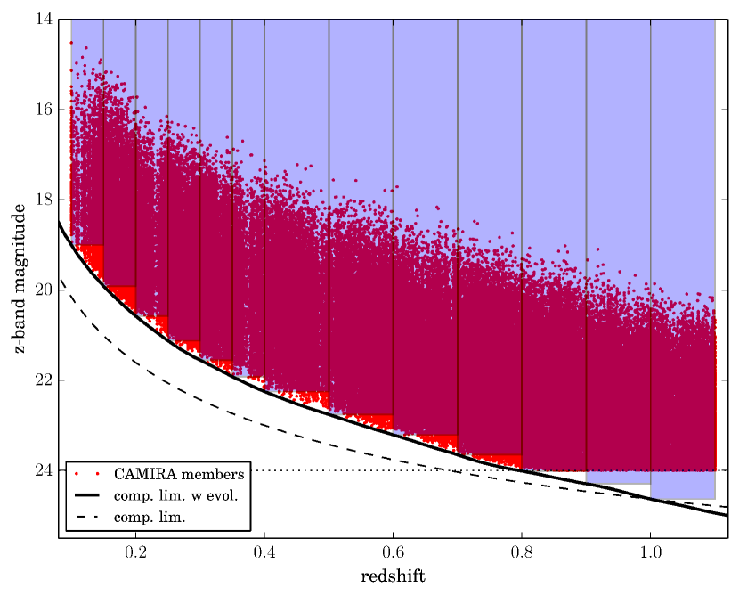
Figure 1: Redshift and magnitude distribution of all CAMIRA member galaxies. The dashed line represents the observer-frame $z$-band magnitude of a SPS with constant absolute magnitude $M_{z}$=-18.5 as seen at different redshifts. The thick solid line is the same constant absolute magnitude but after applying $K$-correction and taking into account passive evolution. Shaded rectangles are regions where the galaxy sample is complete and suitable for exploring the redshift evolution of clusters in various aspects over different redshifts. The horizontal dotted line represents the $m_{z}=24.0$ mag cut that we apply to remove the galaxies affected by large photometric errors especially in the highest redshift bins of the cluster sample (see Section 2.3 for details).

redshift bin	mean redshift	color	number of clusters
0.10–0.15	0.13	$g-r$	43
0.15–0.20	0.18	$g-r$	91
0.20–0.25	0.22	$g-r$	74
0.25–0.30	0.28	$g-r$	145
0.30–0.35	0.32	$g-r$	130
0.35–0.40	0.38	$g-r$	70
0.40–0.50	0.45	$r-i$	192
0.50–0.60	0.55	$r-i$	220
0.60–0.70	0.65	$r-i$	179
0.70–0.80	0.75	$i-y$	231
0.80–0.90	0.85	$i-y$	217
0.90–1.00	0.95	$i-y$	137
1.00–1.10	1.05	$i-y$	173

Table 1: The definition of redshift bins used in this paper. For each redshift bin, the mean redshift of clusters, the color combination used to define red and blue galaxies, and number of clusters with $\hat{N}_{\rm mem}>15$ are shown.

2.3 HSC sample selection

In this Section, we describe our selection of the HSC photometric galaxy sample, which is used for our analysis of the cluster galaxy population. In this paper, we use magnitudes for each object that are derived by combining CModel magnitudes (Abazajian et al., 2004; Bosch et al., 2017) with PSF matched aperture magnitudes, the so-called afterburner photometry (Bosch et al., 2017). The CModel magnitude is obtained by fitting the object light profile with the sum of a de Vaucouleurs bulge and an exponential disk convolved with the PSF. PSFs are measured at the positions of stars and then modeled to interpolate over the entire field of view (Bosch et al., 2017). The PSF-matched aperture magnitude in the afterburner photometry is obtained by stacking the image after blurring each exposure toward the target PSF size and measuring the photometry at a given aperture size. All the magnitudes are corrected for the Galactic extinction (Schlegel et al., 1998). First we define the total magnitude of each galaxy with the $z$-band CModel magnitude. Then we derive the magnitudes in other bands as

$$m_{x}=m_{z}^{\rm CM}+\left({m}_{x}^{\rm ab}-{m}_{z}^{\rm ab}\right),$$ (1)

where ${m}_{z}^{\rm CM}$ is the CModel magnitude in the $z$-band measured with forced photometry on the PSF-unmatched coadd image (cmodel_mag), and ${m}_{x}^{\rm ab}$ (${m}_{z}^{\rm ab}$) is the PSF-matched aperture magnitude in $x$-band ($z$-band) measured in $0\farcs 55$ aperture in radius on the stacked image, where the PSF is convolved to homogenize the target PSF size of $1\farcs 1$ (parent_mag_convolved_2_0). As the error of the afterburner photometry is significantly underestimated because the neighboring pixels are highly correlated due to the blurring, we use the photometric error associated with the PSF-unmatched aperture photometry with a corresponding aperture instead of the afterburner photometry error.

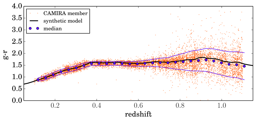
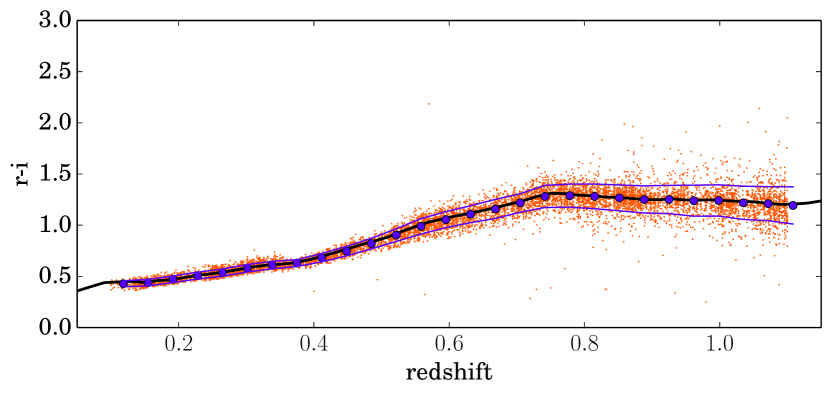
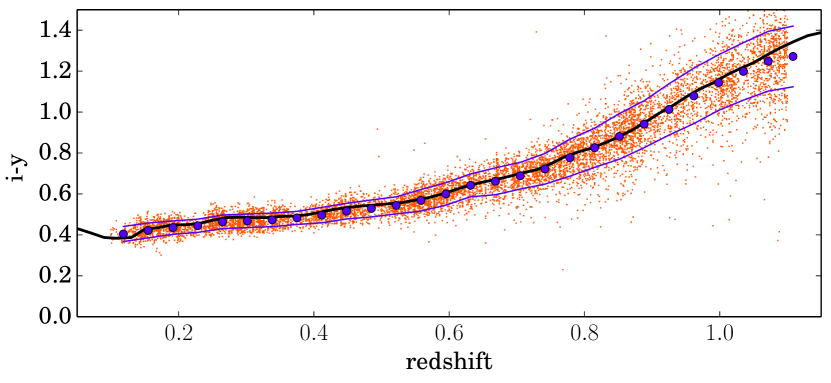
Figure 2: Redshift-color relation of red-sequence galaxies. Red points are cluster member galaxies identified by CAMIRA, and their median and 1$\sigma$ region are denoted by filled circles and thin solid lines. Thick solid line show model colors from the SPS model (Bruzual & Charlot, 2003) calibrated with spectroscopic redshifts.

In the following we describe flags applied to select galaxies with high-quality photometry (Aihara et al., 2017b).
Flags in forced photometry table

• [grizy]flags_pixel_edge is not True

• [grizy]flags_pixel_interpolated_center is not True

• [grizy]flags_pixel_cr_center is not True
  We apply the above three constraints to avoid objects geometrically overlapping with the masked region [EDGE or NO DATA], or object centers close to interpolated pixels or suspected cosmic rays.

• [grizy]cmodel_flux_flags is not True
  These flags ensure that the CModel flux is successfully measured.

• [grizy]centroid_sdss_flags is not True
  Exclude objects for which measurements of centroids failed using the same method as in the Sloan Digital Sky Survey (Bosch et al., 2017).

• [gr]countinputs $>1$

• [izy]countinputs $>3$ In the HSC-Wide, we divide every pointing into 4 for $g$- and $r$-band, and 6 for $i$-, $z$- and $y$-bands. Here we use objects taken twice or more for $g$ and $r$, and four times or more for $i,z$ and $y$ bands.

• detect_is_primary is True
  We also remove blended objects to avoid ambiguous photometric measurements.

• zcmodel_mag - a_z $<24.0$
  We limit our sample in these magnitudes ranges so that all the objects have high signal to noise ratio.

• rcmodel_mag - a_r $<28.0$

• icmodel_mag - a_i $<28.0$ These two flags are not for the primary object selection but for removing too faint objects.

• zcmodel_mag_err $<0.1$
  We also directly impose the $S/N$ cut corresponding to $S/N\gtrsim 10$.

• iclassification_extendedness $=1$
  Stars are excluded.

Flags in afterburner table

• [grizy]parent_flux_convolved_2_0_flags is not True

In addition to the above selection, we use only galaxies brighter than the limits shown in Figure 1 depending on the redshift of clusters.

As a sanity check, we compare colors of CAMIRA cluster member galaxies with model colors from the SPS model used in CAMIRA cluster finding (Oguri et al., 2017), which is based on the SPS model of Bruzual & Charlot (2003) with the calibration of colors from spectroscopic redshifts as described above. Figure 2 shows the redshift evolution of colors of CAMIRA cluster member galaxies, where we derive colors of cluster member galaxies by matching the photometric galaxy sample constructed above with a catalog of CAMIRA member galaxies from Oguri et al. (2017). We find that model colors and median colors of the member galaxies agree well, as expected. As shown in Figure 2, in the redshift ranges of $0.1<z<0.4$, $0.4<z<0.7$, $0.7<z<1.1$, $g-r$, $r-i$, and $i-y$ respectively show rapid color changes, because these colors cover the $4000\AA$ break at these redshifts. Moreover, we find that the above combination of filters shows the tightest scatter around the theoretical prediction in each redshift range. Therefore, we use these colors to construct the color magnitude diagram to see the red-sequence galaxies at fainter magnitude with a stacking analysis (see Table 1).

3 Statistical identification of cluster member galaxies

3.1 Stacking analysis

In this paper, we study distributions of cluster member galaxies statistically, without resorting to spectroscopic or photometric redshifts. Since we do not use both photometric redshift and spectroscopic redshift for each galaxy, physical quantities of individual galaxies such as stellar masses or star formation rates are not available; however, an advantage of our approach is that we can exclude any uncertainties associated with photometric redshift measurements, which may also induce uncertainties in identification of cluster member galaxies. This statistical method has been used previously in the literature (e.g. Lin et al., 2004; Hansen et al., 2005; Loh & Strauss, 2006). Here we describe our specific procedure.

First we divide the CAMIRA cluster catalog into subsamples at different redshift bins, as shown in Table 1. In each redshift bin, we have roughly $\sim 50-200$ clusters. The galaxy distribution associated with the $i$-th cluster and $j$-th annulus can be written as

$$N_{ij}^{\rm in}(z_{\rm cl})=\sum_{k}\Theta(|\Delta{\boldsymbol\theta}_{ik}|\chi_{{\rm cl},i}-r_{P,j})\Theta(r_{P,j+1}-|\Delta{\boldsymbol\theta}_{ik}|\chi_{{\rm cl},i}),$$ (2)

where the summation $k$ runs over galaxies, $\chi_{\rm cl}$ is comoving distance to the cluster redshift $z_{\rm cl}$, $\Delta{\boldsymbol\theta}_{ik}$ is the sky separation of the $k$-th galaxy with respect to the $i$-th cluster center, and $\Theta$ is a Heaviside step function. We consider the comoving radial distance from the cluster center $r_{P}$ in the range from 0.1 to 5 $h^{-1}{\rm Mpc}$ (comoving), which is divided into 15 logarithmically uniform bins. After stacking over all clusters within each redshift bin, we have

$$N_{j}^{\rm in}(r_{P})=\sum_{i}N_{ij}^{\rm in}.$$ (3)

This number $N_{j}^{\rm in}$ includes not only cluster member galaxies but also foreground and background galaxies along the line of sight. In order to remove these foreground and background galaxies, we assume that the galaxy number distribution outside the cluster region defined by $r=|\Delta{\boldsymbol\theta}_{ik}|\chi_{{\rm cl},i}>5h^{-1}{\rm Mpc}$ well represents the distribution of the foreground and background galaxy population. Although the distribution may differ field by field due to both inhomogeneous observing conditions and large-scale structure of the Universe, such local variation of the galaxy number distribution is expected to be averaged out after stacking many clusters at different positions on the sky, as long as the sky coverage of the survey is sufficiently large (e.g., Goto et al., 2003). The galaxy number outside the cluster region $N^{\rm out}$ for each redshift bin is estimated by using all galaxies that are located at $r>5h^{-1}{\rm Mpc}$ for all the clusters in the redshift bin. The number of galaxies is rescaled by the area before subtraction. We then subtract the contamination by foreground and background galaxies using $N^{\rm out}$ estimated above. We measure the areas occupied by the galaxies outside the cluster regions by counting the number of randoms in the random catalog (Coupon et al., 2017). The random catalog is created based on the pixel-based information and inherits most of the photometric flags on the object images. One can find the corresponding version of random catalog to the object catalog in the same data release site. The random catalog takes account of both the selection criteria described in Section 2.3 and masks. Now the foreground and background subtracted number of galaxies can be written as,

$$N_{j}=N^{\rm in}_{j}-N^{\rm out}\frac{R^{\rm in}_{j}}{R^{\rm out}},$$ (4)

where $R$ is the number of randoms which is defined in the exactly same manner as in equations 2 and 3.

3.2 Color correction

As shown in Figure 2, the tight relation of red-sequence evolve with redshift. This means that galaxy colors evolve with redshift, even within the same redshift bin. In order to obtain accurate stacking results, including accurate separation of red and blue galaxies based on their colors, we apply a correction for the color evolution as a function of redshift before stacking many clusters to study the population of red and blue galaxies within each redshift bin. For clusters at $z=z_{1}$, we derive the corrected color as $C_{\rm corr}=C_{\rm obs}-C^{\rm th}(z_{1})+C^{\rm th}_{\star}$, where $C^{\rm th}$ denotes the theoretically derived galaxy color based on the stellar population synthesis model of Bruzual & Charlot (2003) with the calibration of colors using spectroscopic galaxies in the HSC survey (Oguri et al., 2017). $C_{\star}^{\rm th}$ is $C^{\rm th}$ at the median redshift $z_{\star}$ within the redshift bin. Furthermore, we correct the color gradient as a function of magnitude using $z$-band magnitudes. We fit the colour-magnitude relation along the red sequence by the linear function as $g(m_{z})=g_{\star}+\alpha(m_{z}-m_{z,\star})$, and correct the colors of all galaxies to the red-sequence zero-point (intercept of the linear relationship) estimated at the median magnitude of the cluster member galaxies, $g_{\star}\equiv g(m_{z,\star})$.

To summarize, the corrected color of a galaxy with magnitude $m_{z}$ for a cluster at $z_{\rm cl}$ stands for the color difference from that of the red sequence and is derived from the observed raw color $C_{\rm obs}$ as

$$C(m_{z}|z_{\rm cl},m_{z,\star})=C_{\rm obs}-C^{\rm th}(z_{\rm cl})+C^{\rm th}_{\star}-g(m_{z})+g_{\star}.$$ (5)

We show the color gradient in terms of redshift in Figure 2 for CAMIRA member galaxies and the color gradient in terms of z-band magnitude in Figure 3.

3.3 Definition of Red and Blue galaxies

While there are a variety of definitions of red and blue galaxies in the literature, we introduce an empirical definition based on the observed data. Since CAMIRA cluster member galaxies represent the population of quiescent galaxies, the location of the CAMIRA cluster member galaxies in the CMD is well localized. This means, at a given redshift, galaxies having different star formation activities have different colors. We define blue galaxies as those that are located in the CMD 2$\sigma$ away (on the bluer side) from the linear relation of the red-sequence obtained in Section 3.2. Figure 3 shows CMD after the foreground and background subtracted in different redshifts (low-z to high-z from top to bottom) and different cluster centric radius (inner to outer from left to right). The color tilts are not corrected (but see Fig. 4 for color corrected diagram for $z=0.55$ and $r_{P}<0.5h^{-1}{\rm Mpc}$). Horizontal dashed lines are the location dividing the sample into red and blue galaxies. It is clearly seen that there are few blue galaxies at inner region of clusters and it increases with the cluster centric radius. We will see this more in detail in Section 5. We note that if we carefully focus on the faint end of the CMD, the linear function obtained by CAMIRA member galaxies are slightly off from the peak of the red galaxies distribution. Unlike the CAMIRA member galaxies which are well matured to be red sequence, faint galaxies near the red-sequence track still in the stage of star forming and in the transition phase from star forming galaxies to quiscent galaxies. For the thorough investigation, we need to divide the cluster sample in finner mass bins, which will be devoted to our future paper.

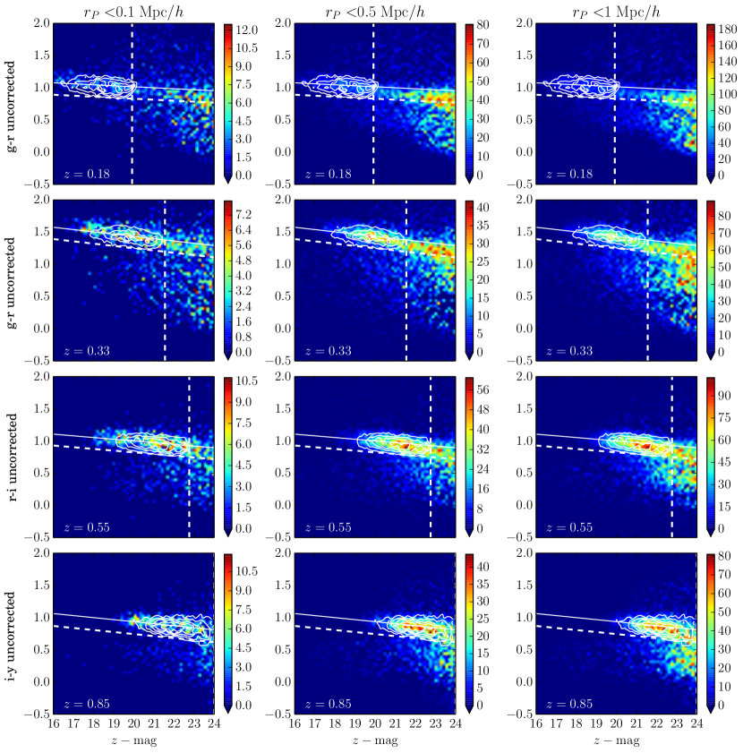
Figure 3: Color-magnitude diagrams (CMDs) that are derived by stacking photometric galaxies over all CAMIRA clusters. Color level stands for the number of galaxies in each cell after foreground and background galaxies are statistically subtracted (see the text for details). From left to right, we show CMDs for the cluster centric radius $r_{P}<0.1,0.5$ and $1.0h^{-1}{\rm Mpc}$. From top to bottom, the mean redshift of the clusters are $z_{\rm cl}=0.18$, $0.33$, $0.55$, and $0.85$. Overlaid contours in each panel are the distribution of cluster member galaxies identified by CAMIRA. Solid lines show the slopes that minimize the scatter of CAMIRA member galaxies around the line, i.e. $g(m_{z})$ correction. We define red and blue galaxies for each redshift bin by those above and below the dashed line (which is defined by a line 2$\sigma$ below the solid line), respectively. Vertical dotted lines are the apparent magnitude cut corresponding to the rest frame $M_{z}<-18.5$.

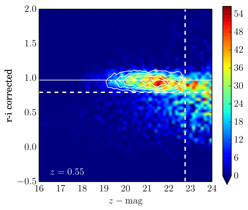
Figure 4: Same as Fig. 3 for $z=0.55$ and $r_{P}<0.5h^{-1}{\rm Mpc}$, but color is corrected according to equation 5.

4 Red-sequence at the Faint End

In this Section, we study the red-sequence galaxies within cluster centric radius $r_{P}<0.5h^{-1}{\rm Mpc}$ at the very faint end down to $m_{z}\sim 24$, which is enabled by our careful statistical subtraction of foreground and background galaxies. Specifically, we study how the scatter of the red-sequence changes as a function of magnitude. We model the color-corrected, foreground and background-subtracted CMD distribution with the following double Gaussian (e.g. Hao et al., 2009)

$$n(C|m_{z})=\frac{A_{R}(m_{z})}{\sqrt{2\pi\sigma_{R}^{2}(m_{z})}}\exp\left[-\frac{(C-C_{R})^{2}}{2\sigma_{R}^{2}(m_{z})}\right]+$$

$$\hskip 80.00012pt\frac{A_{B}(m_{z})}{\sqrt{2\pi\sigma_{B}^{2}(m_{z})}}\exp\left[-\frac{(C-C_{B})^{2}}{2\sigma_{B}^{2}(m_{z})}\right]$$ (6)

where the parameters $A_{x},\sigma_{x}$ and $C_{x}$ with $x$ being either $R$ (red) or $B$ (blue), are treated as free parameters. As we already corrected for the color tilt against the magnitude in Section 3.2, the mean of the red component, $C_{R}$, can well be described by a constant. For simplicity, we also assume that the blue component has constant mean ($C_{B}$), which is equivalent to assuming that the tilt of the color-magnitude relation for blue galaxies is the same as that for red galaxies. This assumption is reasonable because the blue galaxies do not have tight relation with the $m_{z}$ but are rather broadly distributed and thus insensitive to the choice of color correction; as far as the tilt correction is linear, the color correction simply changes the $C_{B}$ and $\sigma_{B}$ at each $m_{z}$ bin but it does not affect the estimate of $\sigma_{R}$ we are interested in. We divide the CMD in several magnitude bins, and estimate the values of $\sigma_{R}$ for each magnitude bin with Markov-Chain Monte-Carlo method by keeping other parameters free but fixing the $C_{R}$ to its corrected value obtained in Section 3.2.

Figure 5 shows the best fit scatter parameter $\sigma_{R}$ as a function of magnitude, for different cluster redshifts. As discussed above, we use different colors for clusters at different redshift, such that these colors refer to approximately the same color in the cluster rest frame. At the very faint end, we need to take account of the scatter associated with the photometric error, which has a significant contribution to the observed scatter at $m_{z}\sim 24$. As the intrinsic scatter is not correlated with the photometric error, we can separate their contributions as

$$\sigma_{\rm obs}^{2}=\sigma_{\rm photo}^{2}+\sigma_{\rm int}^{2},$$ (7)

where $\sigma_{\rm obs},\sigma_{\rm photo}$ and $\sigma_{\rm int}$ are the observed scatter, the scatter due to the photometric error, and the intrinsic scatter of the red-sequence, respectively. We find that the intrinsic scatter of the red-sequence galaxies after subtracting the photometric error is almost constant over wide range of magnitudes. We also find that there is no significant redshift evolution of the scatter, which is consistent with the previos work using smaller sample of clusters (e.g., Cerulo et al., 2016; Hennig et al., 2017). The Figure suggests a slight decrease of the scatter at the faint end, but being the photometric error large at faint magnitudes, the intrinsic scatter is likely to be underestimated. Over most of the magnitude range, however, the photometric error is much smaller than the intrinsic scatter, which indicates that our result is robust against the photometric error.

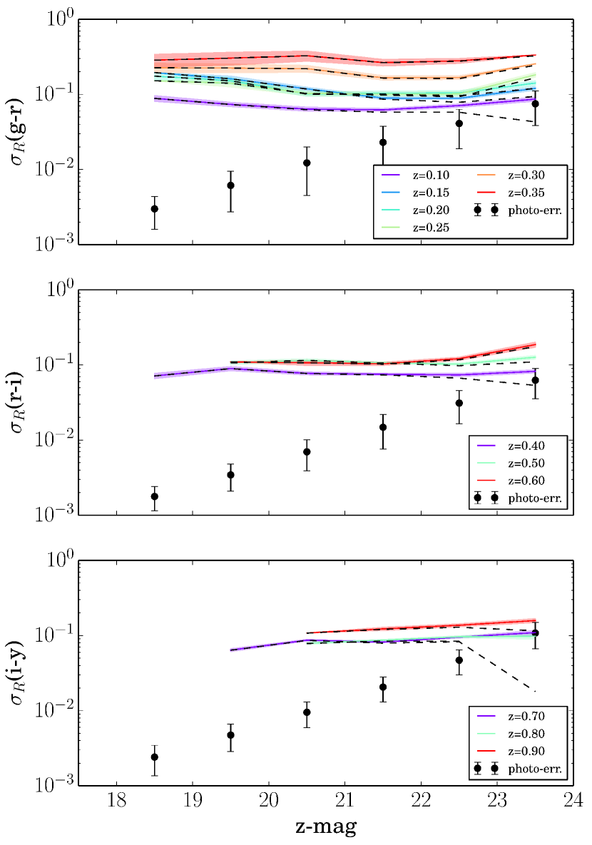
Figure 5: The scatter of colors of red-sequence galaxies as a function of $z$-band magnitude. Results are shown for different redshift bins. Shaded regions show observed scatter, whereas dashed lines show the estimated intrinsic scatter after subtracting the scatter due to the photometric error which is shown by filled circles with errorbars. The circles and errorbars are median and one sigma scatter of the photometric error in each magnitude bin.

5 Cluster Profile and Fraction of Red galaxies

5.1 Cluster Profile

Given the timescale for the evolution of galaxies, tracking the redshift evolution of the number density profiles for red and blue components can help us understand the dynamical history of the formation of galaxy clusters. The radial mass density profile of dark matter halos has long been thought to have a long tail that goes like $\rho\propto r^{-3}$ Navarro et al. (1996). With such a profile, the total enclosed mass of a cluster diverges logarithmically, and the total mass associated with the halo depends upon the arbitrary boundary imposed on the halo. The splashback radius, marked by the apocenter of the recently infalling material, provides a clear physical boundary for the halo and can be used to identify the edges of dark matter halos (Diemer & Kravtsov, 2014; More et al., 2015). The splashback radius manifests itself as a sharp drop in the matter density at its location (Diemer & Kravtsov, 2014; Adhikari et al., 2014). The dark matter profile with such a density jump can be modeled with an inner universal profile multiplied by a transition function and an outer profile which represents the so-called two-halo contribution (Diemer & Kravtsov, 2014). This can be explicitly written as

$$\rho(r)=\rho^{\rm in}(r)\left[1+\left(\frac{r}{r_{t}}\right)^{\beta}\right]^{-\gamma/\beta}+\rho^{\rm out}(r),$$ (8)

$$\rho^{\rm out}(r)=\rho_{m}\left[b_{e}\left(\frac{r}{5R_{200}}\right)^{-s_{e}}+1\right],$$ (9)

where $r_{t},\gamma$ and $\beta$ denote the location of the dip in the profile, the steepness of the dip and how rapidly the slope changes, respectively. They all characterize the transition between inner and outer profiles. For the outer profile, $\rho_{m},b_{e}$ and $s_{e}$ represent the overall normalization, relative normalization of power law profile and index of the power law, respectively. Diemer & Kravtsov (2014) express $r_{t}/R_{\rm 200m}$ as a function of the accretion rate $\Gamma$ as $r_{t}/R_{\rm 200m}=(0.62+1.18\exp[-2\Gamma/3])$, but in this paper we keep $r_{t}$ as a free parameter since we do not have reliable estimate of the either the $R_{\rm 200m}$ or the accretion rate of our optically-selected clusters. We use the NFW (Navarro et al., 1996) profile to describe the inner profile,

$$\rho^{\rm NFW}(r)=\frac{\rho_{s}}{(r/r_{s})(1+r/r_{s})^{2}},$$ (10)

where $r_{s}$ and $\rho_{s}$ denote the transition scale of slope from $-1$ to $-3$ and overall normalization, respectively. While we use $r_{t}$ for fitting observed radial profiles, following More et al. (2015) we define a splashback radius, $R_{\rm sp}$, as the radius where the radial profile attains its steepest slope. As in More et al. (2016), we allow $\beta$ and $\gamma$ to take the values with $\log\beta=\log 6\pm 0.2$ and $\log\gamma=\log 4\pm 0.2$. The profiles of equations 8, 9 and 10 are numerically integrated along the line of sight to project to the two-dimensional sky.

Figure 6 show the radial number density profiles for red and blue components at redshifts $z=0.18$, $0.33$, $0.55$, and $0.85$. The covariance matrices are estimated from the jackknife resampling as

$$\widehat{{\rm Cov}_{ij}} = \frac{N_{a}-1}{N_{a}}\sum_{a}[w_{a}^{\rm cg}(r_{{\rm p},i})-\overline{w^{\rm cg}}(r_{{\rm p},i})]\times$$ (11)

$$\hskip 60.00009pt[w_{a}^{\rm cg}(r_{{\rm p},j})-\overline{w^{\rm cg}}(r_{{\rm p},j})],$$

where $\overline{w^{\rm cg}}$ is the arithmetic mean of $w^{\rm cg}_{a}$. We divide the entire area into 35 rectangular regions with a side of $5.0$ deg. That scale corresponds to the comoving angular separation of $25h^{-1}{\rm Mpc}$ at $z=0.1$ which is sufficiently larger than the scale of our interest and includes more than one cluster in all sub-divided regions. We first fit to an NFW profile by restricting to scales below $1h^{-1}{\rm Mpc}$. Best-fit scale radii are summarized in the Table 2. We find notable differences of concentrations between two populations. Red galaxies are more concentrated toward the cluster center (i.e., smaller $r_{s}$) and blue galaxies are less concentrated (i.e., larger $r_{s}$). The difference in the concentration can be accounted for by the merger of clusters as discussed in (e.g Okamoto & Nagashima, 2003, 2001). Another possible explanation is that red galaxies at the same luminosity live in more massive halos than their blue counterparts (Mandelbaum et al., 2006; More et al., 2011) and have experienced more dynamical friction so that they are concentrated toward the cluster center as we see in the discussion below. If we focus on the redshift evolution, it is seen that the overall profile tends to be more concentrated for lower redshifts. While the evolution of the concentration of red galaxies is subtle, blue galaxies evolve rapidly from $z=0.5$ to $0.3$.

Next we fit all the data to the full profile of equation (8), keeping $r_{s}$ and $\rho_{s}$ fixed to their best fit values from the simple NFW profile fitting to simplify the degeneracies inherent in the fitting procedure. The best fit curves are presented with solid lines in Figure 6. We also show the logarithmic slope of the profile, which can be used to define the splashback radius $R_{\rm sp}$ as a local minimum of the slope. We compare the splashback radii $R_{\rm sp}$, $r_{t}$, and $r_{s}$ in Table 2.

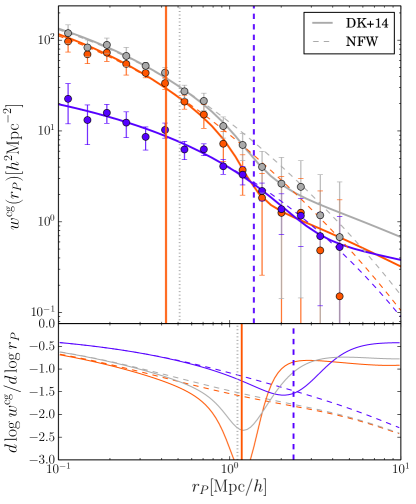
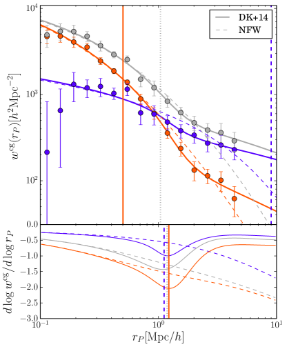
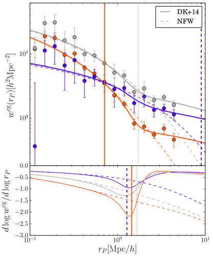
Figure 6: Radial number density profiles of galaxies around clusters. From left to right, the mean redshifts of clusters are 0.18, 0.33, 0.55, and 0.85. Red and blue symbols show profiles for red and blue member galaxies. Gray symbols show profiles for all galaxies. Dashed lines are best-fit models of the projected NFW profile. Solid lines show the best-fit Diemer & Kravtsov (2014) model. Vertical solid and dashed lines indicate the best-fit scale radii $r_{s}$ for red and blue galaxies, respectively. Bottom panels show the slope of the best-fit profiles with vertical lines being the best-fit value of $r_{t}$, which can be compared with the splashback radius, $R_{\rm sp}$.

$z$	sample	$r_{s}$	$r_{t}$	$R_{\rm sp}$	$\Delta$AIC	$\Delta$BIC
	red	0.50$\pm$0.01	1.20$\pm$0.13	1.21$\pm$0.70	-15.1	-10.9
0.18	blue	1.14$\pm$0.03	3.63$\pm$1.07	2.66$\pm$1.29	-16.3	-12.2
	all	0.57$\pm$0.01	1.11$\pm$0.13	1.21$\pm$0.66	-15.3	-11.1
	red	0.51$\pm$0.01	1.34$\pm$0.16	1.26$\pm$0.66	-16.2	-12.1
0.33	blue	8.61$<$	1.43$\pm$0.18	1.52$\pm$0.58	-17.1	-12.9
	all	0.91$\pm$0.02	1.53$\pm$0.22	1.15$\pm$0.64	-16.6	-12.4
	red	0.54$\pm$0.01	1.20$\pm$0.10	1.26$\pm$0.73	-15.7	-11.6
0.55	blue	8.42 $<$	1.20$\pm$0.18	1.26$\pm$0.54	-16.1	-11.9
	all	1.11$\pm$0.03	1.12$\pm$0.12	1.10$\pm$0.52	-15.5	-11.3
	red	0.77$\pm$0.03	1.40$\pm$0.13	1.32$\pm$0.79	-17.2	-13.1
0.85	blue	7.73 $<$	1.75$\pm$0.47	1.67$\pm$0.54	-17.3	-13.1
	all	1.72$\pm$0.12	1.29$\pm$0.27	1.21$\pm$0.39	-17.3	-13.2

Table 2: Best-fit values of cluster profile parameters. For each redshift range, the top, middle and bottom rows are for red galaxy, blue galaxy and all galaxy samples, respectively. All the values are in comoving $h^{-1}{\rm Mpc}$. Also shown are difference of information criteria. Minus value means that the NFW profile is favored over density jump model.

As shown in More et al. (2015), there is a tight relation between the mass accretion rate of clusters and the normalized splashback radius $R_{\rm sp}/R_{200m}$ obtained by stacking clusters at each redshift. Given the fact that the richness limit of our cluster sample approximately corresponds to a constant mass limit of $M_{200m}>10^{14}h^{-1}{\rm M}_{\odot}$ over the whole redshift range (Oguri et al., 2017), we find that the splashback radii from our fits roughly correspond to $R_{\rm sp}\sim R_{\rm 200m}$. This is broadly consistent with More et al. (2016) in which splashback radii were derived for Sloan Digital Sky Survey (SDSS) clusters to argue that the observed splashback radii are smaller than the standard cold dark matter model prediction, implying the faster mass accretion than the standard model. However more careful estimates of the mass of these clusters using the weak gravitational lensing signal ought to be performed before doing a more quantitative comparison to More et al. (2016) as well as to quantify the redshift evolution. We will explore this in the near future.

We compare the goodness of fit between NFW and full profile of Diemer & Kravtsov (2014) by computing two different criteria; Akaike Information Criteria (AIC) corrected for the finite data size and Bayesian Information Criteria (BIC). They are defined as

$$\displaystyle{\rm AIC} = -2\ln({\mathcal{L}})+2p+\frac{2p(p+1)}{N-p-1}$$ (12)

$${\rm BIC} = -2\ln({\mathcal{L}})+\ln(N)p,$$ (13)

where ${\mathcal{L}}$ is the likelihood and $p$ and $N$ are number of parameters and data, respectively; $(N,p)$ for NFW is $(9,2)$ and $(15,6)$ for density jump model. We compare the information criteria for two profile fittings, and find that the density jump model is disfavored as summarized in Table 2.

As a cautionary note, we also mention that selection effects in optical cluster finding can significantly complicate the inference of the splashback radius from observations. Optical clusters are more likely to have their major axis oriented along the line-of-sight which break the spherical symmetry assumption involved in the inference of the splashback radius (see e.g., Busch & White, 2017). In addition degeneracies related to cluster miscentering can also reduce the significance of the detection of the splashback radius (Baxter et al., 2017). The values of the splashback radii inferred from optical clusters should therefore be carefully compared to expectations, a topic we will focus on in the near future.

For clusters at $z>0.5$, we find a slight decline of radial profiles in the central region, $r<0.2h^{-1}{\rm Mpc}$. This might reflect the mis-centering of the optically-selected clusters, which have been inferred in comparison with the X-ray profile (Oguri et al., 2017). It may be more difficult to correctly identify the center of cluster at higher redshift simply because in crowded regions, like cluster centers, angular separations of neighboring galaxies are smaller at higher redshifts given the same physical scale. This is mainly due to the fact that the pipeline fails to deblend galaxies in crowded regions. We leave the effect of mis-centering for future work, after the weak lensing measurement of the CAMIRA cluster sample becomes available.

5.2 Red fraction as a function of redshift

We derive the red galaxy fraction by summing up the number of red and blue galaxies in each radial bin out to the maximum comoving distances, for which we adopt $0.2$, $0.5$, and $1.0h^{-1}{\rm Mpc}$. Figure 7 shows the evolution of fractions of red galaxies as a function of redshift, for three different maximum distances. We can clearly see the evolution of the red fraction over the cosmological time scale, from $z=1.1$ to $0.1$, such that the red fraction increases at lower redshift. This qualitative trend is consistent with Hennig et al. (2017); Jian et al. (2017), while Loh et al. (2008) reported steeper evolution. The red fraction significantly increases with decreasing maximum distance from the cluster center, which is due to the different radial number density profiles between red and blue galaxies. We note that there are gaps in the fraction of red galaxies at $z=0.4$ and $z=0.75$ because we have used the different combination of filters to define red and blue galaxies. This implies that the global evolution of red fraction over the redshifts $0.1<z<1.1$ is subject to the choice of colors; however, within the redshift range in which we use the same filter combination, we observe apparent decreases of the red fraction. However, we note that the red fraction at higher redshift bins, $0.7<z$, are almost flat or slight increasing. As we will discuss it at the end of the Section 5.3, this trend is partly due to our bad photometry at crowded region like cluster center.

Figure 8 shows the fraction of red galaxies as a function of projected cluster-centric radius $r_{\rm P}$. Symbols are observed points and solid lines are predictions from the semi analytical model described in Section 5.3. The fractions of red galaxies are high, $\sim 0.6-1.0$ in the inner regions ($r_{\rm P}<0.3h^{-1}{\rm Mpc}$), decreasing to $\sim 0.2-0.4$ in the outer regions ($r_{\rm P}>1h^{-1}{\rm Mpc}$). On the intermediate scale in between the inner and outer regions, the fraction of red galaxies is gradually decreasing. Although the absolute value of the observed fraction is slightly higher than predicted by the semi analytical model, the declining slopes are in good agreement with the model.

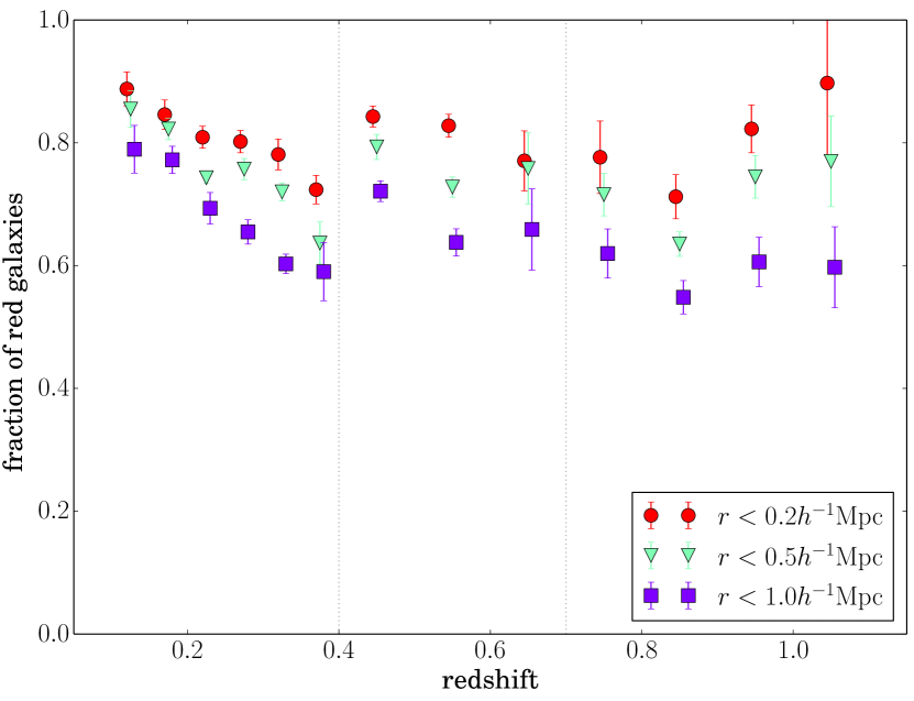
Figure 7: Fraction of the red galaxies as a function of redshift and the maximum distance from the cluster center for counting up the galaxies. The x-axis for different $r_{P}$ is slightly shifted for visual purpose.

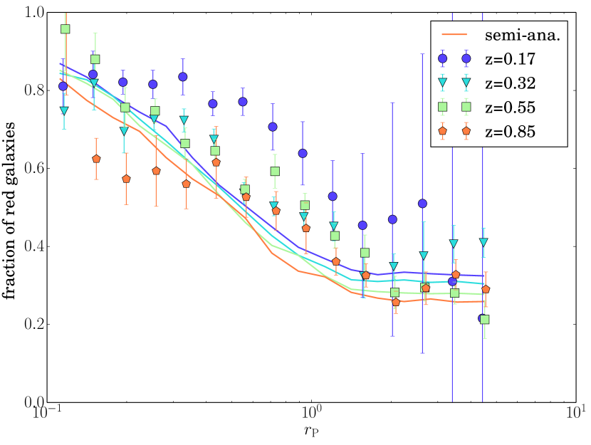
Figure 8: Radial profile of the fraction of red galaxies as a function of projected cluster-centric radius at four different redshifts. Symbols are observed data points and solid lines are the prediction from the semi-analytical model described in Section 5.3.

5.3 Comparison with Semi Analytical Model

It is important to check the consistency of our results with theoretical models of galaxy formation. We compare our results with a semi-analytical model of galaxy formation, $\nu^{2}$GC (Makiya et al., 2016). Semi-analytical models have an advantage over mock galaxy catalogs based on the halo occupation distribution technique in that semi-analytical models are constructed from physically motivated prescriptions of several astrophysical processes which, in comparison with observations, will lead to better understanding of the build-up of cluster galaxies. They also contain physical properties of galaxies such as galaxy stellar and gas masses and star formation rates. The information may also help reveal physical processes affecting evolution of cluster galaxies.

We examine the spatial distribution of galaxies in $\nu^{2}$GC. In $\nu^{2}$GC, we construct merger trees of dark matter halos using cosmological $N$-body simulations (Ishiyama et al., 2015) with the Planck cosmology (Planck Collaboration et al., 2014). The simulation box is 280 $h^{-1}{\rm Mpc}$ on a side containing $2048^{3}$ particles, corresponding to a particle mass of $2.2\times 10^{8}h^{-1}M_{\odot}$. The semi-analytical model includes the main physical processes involved in galaxy formation: formation and evolution of dark matter halos; radiative gas cooling and disc formation in dark matter halos; star formation, supernova feedback and chemical enrichment; galaxy mergers; and feedback from active galactic nuclei. The model is tuned to fit the luminosity functions of local galaxies (Driver et al., 2012) and the mass function of neutral hydrogen (Martin et al., 2010). The model well reproduces observational local scaling relations such as the Tully-Fisher relation and the size-magnitude relation of spiral galaxies (Courteau et al., 2007).

We use $\nu^{2}$GC results to create mock galaxy catalogs. Rest-frame and apparent magnitudes of galaxies are estimated in the same filter as used in the HSC survey (Kawanomoto et al., 2017). We apply the same magnitude cut of the HSC ($M_{z}<-18.5$ in rest frame) to the simulated galaxies. In the analysis in this paper, we extract galaxy samples at different redshifts, residing in dark matter halos with mass more than $10^{14}M_{\odot}$. We regard those galaxies as cluster galaxies. We have $\sim 175$ simulated clusters at $z=1.1$ and $\sim 1000$ clusters at $z=0.13$ which are defined in a same realization.

Since the mock catalogs do not perfectly reproduce the colors of galaxies, we cannot apply the selection condition that is applied to the HSC data to the mock catalogs. We therefore re-define the selection criterion for red and blue galaxies in the mock galaxy catalogs. To define red and blue galaxy populations, we determine the red-sequence using a subsample of the mock galaxies as follows. We perform linear regression to fit the slope $\alpha$ and zero-point $\beta$ of the following equation to describe the red sequence

$$C=\alpha\ m_{z}+\beta,$$ (14)

where $C$ is the color corresponding to the cluster redshift, e.g. $g-r$ at redshift [0.1–0.2]. To reduce contaminations by blue galaxies, we only fit to galaxies with specific star formation rate (sSFR) $\log_{10}(\mathrm{sSFR}/\mathrm{Gyr}^{-1})\leq-1$ and with distances from the cluster center $d\leq 0.1~{}\mathrm{Mpc/h}$. These conditions are reasonable to extract red-sequence galaxies which correspond to the CAMIRA-identified red sequence. Finally, in exactly the same manner as in the observation, we define galaxies redder than $C-2\sigma$ line on the CMD as red galaxies, where $\sigma$ is the standard deviation of the distribution of the galaxies used to the fitting.

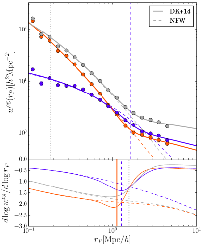
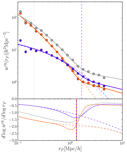
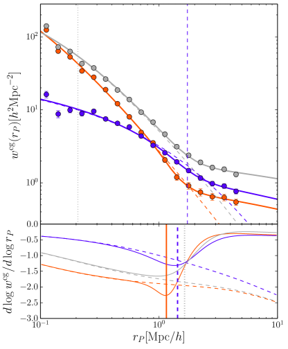
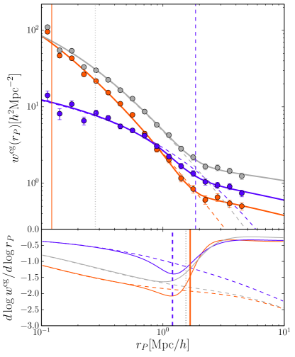
Figure 9: Same as Figure 6 but obtained from simulations with a semi-analytical model.

Figure 9 shows radial profiles of cluster member galaxies for different redshift bins and different populations identified in the simulation. We clearly see that blue galaxies are more diffuse and red galaxies are more concentrated, which is consistent with our observational results.

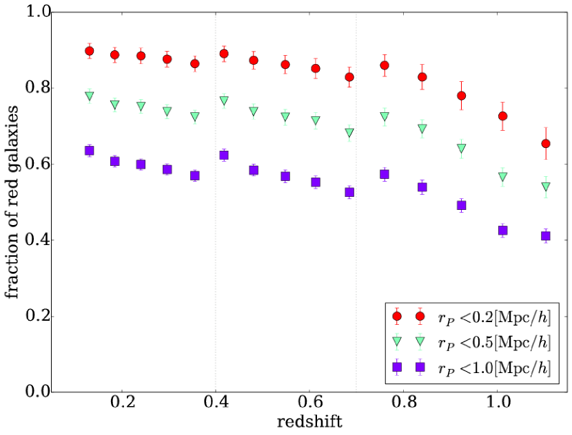
Figure 10: Same as Figure 7 but obtained from simulations with a semi-analytical model.

Figure 10 shows the redshift evolution of the red fraction in the simulation with same binning of distance from the cluster center. We see a clear decrease of the red fraction with redshift and the result shows a reasonable agreement with the observation except for the two highest redshift bins. The simulated results show a monotonic decrease of the red fraction at the highest redshift ranges, but our observational results show a slight increase. The monotonic decrease of the red fraction to $0.5$ at $z=1$ is consistent with the results of Hennig et al. (2017), and therefore the slight increase seen in our data may not be accounted for by the difference in the depth of the sample, (our sample is $\sim 1$ mag deeper in z-band) or the different filter combination used to define the red and blue populations. We do not make strong conclusions about the source of this discrepancy in this paper but it may be partly due to the bad photometry in crowded regions, which significantly affects the color of galaxies in clusters. We will revisit the issue and address it in the future work once the photometry of HSC in the crowded regions is improved.

6 Summary

In this paper, we have used the HSC S16A internal data release galaxy sample over $\sim 230$ deg² to explore the properties of cluster galaxies over the wide redshift and magnitude ranges. Clusters are identified by the red-sequence cluster finding method CAMIRA (Oguri, 2014; Oguri et al., 2017). Thanks to the powerful capability of the Subaru telescope to collect light and the good sensitivity of the HSC detector, we can study faint cluster galaxies down to 24th mag in $z$-band. This sample is $\sim 1$ mag deeper than the cluster sample of Hennig et al. (2017) which reaches $m_{\star}+1.2\sim 23.2$ in DES $z$-band at $z=1$. Together with a reliable CAMIRA cluster catalog out to $z=1.1$, the excellent HSC data allows us to continuously track the evolution history of cluster galaxies from $z=1.1$ to the present.

We have used the stacked color-magnitude diagram to divide red and blue galaxies in clusters. We have statistically subtracted background and foreground galaxies after area corrections using the well defined random catalog, which are also available from the HSC database. After subtracting the foreground and background galaxies, color-magnitude relations for red galaxies (red-sequence) and blue clouds are clearly detected over wide ranges in redshift and magnitude. We have used these color-magnitude diagrams for defining red and blue galaxies, studying the tightness of the red-sequence down to very faint magnitudes, and the radial number density profiles of red and blue galaxies. Our results are summarized as follows.

• Red galaxies in clusters follow a clear linear relation in the color-magnitude diagram down to the HSC completeness limit for all redshifts.

• However, we observe a slight offset of the red populations in the cluster from the linear relation determined by the CAMIRA member galaxies. This may be partly due to our sample selection, i.e. a constant mass cut over all redshift ranges and we will revisit it once the cluster mass is well measured with the weak lensing.

• We have measured the intrinsic scatter of the red-sequence as a function of the observed $z$-band magnitude and cluster redshift. We have found that the intrinsic scatter is almost constant over wide range of magnitudes. The intrinsic scatter shows little evolution with redshift.

• Red galaxies are more concentrated toward the cluster center compared with blue galaxies. We have fit the cluster member radial profile at $r<1.0h^{-1}{\rm Mpc}$ to an NFW profile, and find the transition scale $r_{s}$ is significantly smaller for red galaxies than for blue galaxies. Given that the cluster sample has approximately constant mean mass over different redshifts (Oguri et al., 2017), the mildly decreasing $r_{s}$ with redshift implies that the galaxy profiles in clusters become less concentrated at higher redshift. We note, however, that it is important to independently derive the virial mass of the clusters; this will be soon provided by the HSC weak lensing analysis (Mandelbaum et al., 2017). The special care is required that the mass profile measured by weak lensing is for dark matter and this should be different from the profile of member galaxies.

• We have fit the radial number density profiles with the density jump model of Diemer & Kravtsov (2014), and found that the splashback radius $R_{\rm sp}$ defined by the minimum of logarithmic slope is almost constant over the redshift range. However, given the large statistical uncertainties, we do not detect the splashback radius for our current data set.

• The fraction of red galaxies is not only a strong function of the distance from the cluster center but also exhibits a moderate decrease with increasing redshift. We note that the estimated red fraction shows a slight discontinuity at the redshift where the red and blue galaxies are defined in different combination of colors, i.e. $z\sim 0.4$ and $z\sim 0.7$. This discontinuity might reflect that our definition of red and blue galaxies are not optimal near the transition redshifts because the redshift of the 4000$\AA$ break mismatches to the filter response functions of given combination of the color. We note that the same discontinuity is seen also in the simulations.

• We have also compared our results with semi-analytical model predictions. We have found that the observed cluster profiles and the redshift evolution of the red fraction are broadly consistent with the semi-analytical model prediction. Further studies for more quantitative comparisons are important.

The total mass and mass profile of the CAMIRA clusters can be measured by stacked weak lensing. With the help of the mass-richness relation by the forward modeling (Murata et al., 2017), this will allows us to explore more in detail of cluster physical quantities such as virial radius, mass accretion rate and mass dependence of those quantities. We will revisit this in our future work.

We thank the anonymous referee to provide useful comments. AN is supported in part by MEXT KAKENHI Grant Number 16H01096. This work was supported in part by World Premier International Research Center Initiative (WPI Initiative), MEXT, Japan, MEXT as “Priority Issue on Post-K computer” (Elucidation of the Fundamental Laws and Evolution of the Universe) and JICFuS, and JSPS KAKENHI Grant Number 26800093 and 15H05892. SM is supported by the Japan Society for Promotion of Science grants JP15K17600 and JP16H01089. This work was supported in part by MEXT KAKENHI Grant Number 17K14273 (TN). HM is supported by the Jet Propulsion Laboratory, California Institute of Technology, under a contract with the National Aeronautics and Space Administration.

The Hyper Suprime-Cam (HSC) collaboration includes the astronomical communities of Japan and Taiwan, and Princeton University. The HSC instrumentation and software were developed by the National Astronomical Observatory of Japan (NAOJ), the Kavli Institute for the Physics and Mathematics of the Universe (Kavli IPMU), the University of Tokyo, the High Energy Accelerator Research Organization (KEK), the Academia Sinica Institute for Astronomy and Astrophysics in Taiwan (ASIAA), and Princeton University. Funding was contributed by the FIRST program from Japanese Cabinet Office, the Ministry of Education, Culture, Sports, Science and Technology (MEXT), the Japan Society for the Promotion of Science (JSPS), Japan Science and Technology Agency (JST), the Toray Science Foundation, NAOJ, Kavli IPMU, KEK, ASIAA, and Princeton University.

The Pan-STARRS1 Surveys (PS1) have been made possible through contributions of the Institute for Astronomy, the University of Hawaii, the Pan-STARRS Project Office, the Max-Planck Society and its participating institutes, the Max Planck Institute for Astronomy, Heidelberg and the Max Planck Institute for Extraterrestrial Physics, Garching, The Johns Hopkins University, Durham University, the University of Edinburgh, Queen’s University Belfast, the Harvard-Smithsonian Center for Astrophysics, the Las Cumbres Observatory Global Telescope Network Incorporated, the National Central University of Taiwan, the Space Telescope Science Institute, the National Aeronautics and Space Administration under Grant No. NNX08AR22G issued through the Planetary Science Division of the NASA Science Mission Directorate, the National Science Foundation under Grant No. AST-1238877, the University of Maryland, and Eotvos Lorand University (ELTE).

This paper makes use of software developed for the Large Synoptic Survey Telescope. We thank the LSST Project for making their code available as free software at http://dm.lsst.org.

References

- Abazajian et al. (2004) Abazajian K. et al., 2004, AJ, 128, 502
- Adhikari et al. (2014) Adhikari S., Dalal N., Chamberlain R. T., 2014, JCAP, 11, 019
- Aihara et al. (2017a) Aihara H. et al., 2017a, ArXiv e-prints:1704.05858
- Aihara et al. (2017b) Aihara H. et al., 2017b, arXiv e-prints:1702.08449
- Andreon et al. (2014) Andreon S., Newman A. B., Trinchieri G., Raichoor A., Ellis R. S., Treu T., 2014, A&A, 565, A120
- Axelrod et al. (2010) Axelrod T., Kantor J., Lupton R. H., Pierfederici F., 2010, in Proc. SPIE, Vol. 7740, Software and Cyberinfrastructure for Astronomy, p. 774015
- Baxter et al. (2017) Baxter E. et al., 2017, ArXiv e-prints:1702.01722
- Bosch et al. (2017) Bosch J. et al., 2017, ArXiv e-prints:1705.06766
- Bruzual & Charlot (2003) Bruzual G., Charlot S., 2003, MNRAS, 344, 1000
- Busch & White (2017) Busch P., White S. D. M., 2017, ArXiv e-prints:1702.01682
- Butcher & Oemler (1978) Butcher H., Oemler, Jr. A., 1978, ApJ, 219, 18
- Castorina et al. (2014) Castorina E., Sefusatti E., Sheth R. K., Villaescusa-Navarro F., Viel M., 2014, JCAP, 2, 049
- Cerulo et al. (2016) Cerulo P. et al., 2016, MNRAS, 457, 2209
- Coupon et al. (2017) Coupon J., Czakon N., Bosch J., Komiyama Y., Medezinski E., Miyazaki S., Oguri M., 2017, ArXiv e-prints:1705.00622
- Courteau et al. (2007) Courteau S., Dutton A. A., van den Bosch F. C., MacArthur L. A., Dekel A., McIntosh D. H., Dale D. A., 2007, ApJ, 671, 203
- De Lucia et al. (2007) De Lucia G. et al., 2007, MNRAS, 374, 809
- De Propris et al. (2004) De Propris R. et al., 2004, MNRAS, 351, 125
- Diemer & Kravtsov (2014) Diemer B., Kravtsov A. V., 2014, ApJ, 789, 1
- Dressler (1980) Dressler A., 1980, ApJ, 236, 351
- Driver et al. (2012) Driver S. P. et al., 2012, MNRAS, 427, 3244
- Faber (1973) Faber S. M., 1973, ApJ, 179, 731
- Ferreras et al. (1999) Ferreras I., Charlot S., Silk J., 1999, ApJ, 521, 81
- Gallazzi et al. (2006) Gallazzi A., Charlot S., Brinchmann J., White S. D. M., 2006, MNRAS, 370, 1106
- George et al. (2013) George M. R., Ma C.-P., Bundy K., Leauthaud A., Tinker J., Wechsler R. H., Finoguenov A., Vulcani B., 2013, ApJ, 770, 113
- Gilbank et al. (2007) Gilbank D. G., Yee H. K. C., Ellingson E., Gladders M. D., Barrientos L. F., Blindert K., 2007, AJ, 134, 282
- Gladders & Yee (2000) Gladders M. D., Yee H. K. C., 2000, AJ, 120, 2148
- Gladders & Yee (2005) Gladders M. D., Yee H. K. C., 2005, ApJS, 157, 1
- Goto et al. (2003) Goto T. et al., 2003, PASJ, 55, 739
- Hansen et al. (2005) Hansen S. M., McKay T. A., Wechsler R. H., Annis J., Sheldon E. S., Kimball A., 2005, ApJ, 633, 122
- Hao et al. (2009) Hao J. et al., 2009, ApJ, 702, 745
- Hennig et al. (2017) Hennig C. et al., 2017, MNRAS
- Ishiyama et al. (2015) Ishiyama T., Enoki M., Kobayashi M. A. R., Makiya R., Nagashima M., Oogi T., 2015, PASJ, 67, 61
- Ivezic et al. (2008) Ivezic Z. et al., 2008, arXiv e-prints:0805.2366
- Jian et al. (2017) Jian H.-Y. et al., 2017, ArXiv e-prints
- Jurić et al. (2015) Jurić M. et al., 2015, arXiv e-prints:1512.07914
- Kawanomoto et al. (2017) Kawanomoto et al. S., 2017, PASJ in prep.
- Kodama & Arimoto (1997) Kodama T., Arimoto N., 1997, A&A, 320, 41
- Koester et al. (2007) Koester B. P. et al., 2007, ApJ, 660, 221
- Li et al. (2012) Li I. H., Yee H. K. C., Hsieh B. C., Gladders M., 2012, ApJ, 749, 150
- Lidman et al. (2013) Lidman C. et al., 2013, MNRAS, 433, 825
- Lin et al. (2004) Lin Y.-T., Mohr J. J., Stanford S. A., 2004, ApJ, 610, 745
- Lin et al. (2017) Lin et al. Y., 2017, PASJ in prep.
- Loh et al. (2008) Loh Y.-S., Ellingson E., Yee H. K. C., Gilbank D. G., Gladders M. D., Barrientos L. F., 2008, ApJ, 680, 214
- Loh & Strauss (2006) Loh Y.-S., Strauss M. A., 2006, MNRAS, 366, 373
- Magnier et al. (2013) Magnier E. A. et al., 2013, ApJS, 205, 20
- Makiya et al. (2016) Makiya R. et al., 2016, PASJ, 68, 25
- Mandelbaum et al. (2017) Mandelbaum R. et al., 2017, ArXiv e-prints
- Mandelbaum et al. (2006) Mandelbaum R., Seljak U., Kauffmann G., Hirata C. M., Brinkmann J., 2006, MNRAS, 368, 715
- Martin et al. (2010) Martin A. M., Papastergis E., Giovanelli R., Haynes M. P., Springob C. M., Stierwalt S., 2010, ApJ, 723, 1359
- Mints et al. (2017) Mints A., Schwope A., Rosen S., Pineau F.-X., Carrera F., 2017, A&A, 597, A2
- Miyazaki et al. (2017) Miyazaki et al. S., 2017, PASJ in this volume
- More et al. (2015) More S., Diemer B., Kravtsov A. V., 2015, ApJ, 810, 36
- More et al. (2016) More S. et al., 2016, ApJ, 825, 39
- More et al. (2011) More S., van den Bosch F. C., Cacciato M., Skibba R., Mo H. J., Yang X., 2011, MNRAS, 410, 210
- Murata et al. (2017) Murata et al. R., 2017, PASJ in prep.
- Muzzin et al. (2012) Muzzin A. et al., 2012, ApJ, 746, 188
- Navarro et al. (1996) Navarro J. F., Frenk C. S., White S. D. M., 1996, ApJ, 462, 563
- Oguri (2014) Oguri M., 2014, MNRAS, 444, 147
- Oguri et al. (2017) Oguri M. et al., 2017, arXiv e-prints:1701.00818
- Okamoto & Nagashima (2001) Okamoto T., Nagashima M., 2001, ApJ, 547, 109
- Okamoto & Nagashima (2003) Okamoto T., Nagashima M., 2003, ApJ, 587, 500
- Planck Collaboration et al. (2014) Planck Collaboration et al., 2014, A&A, 571, A16
- Planelles et al. (2015) Planelles S., Schleicher D. R. G., Bykov A. M., 2015, Space Sci. Rev., 188, 93
- Postman et al. (2005) Postman M. et al., 2005, ApJ, 623, 721
- Romeo et al. (2016) Romeo A. D., Cerulo P., Xi K., Contini E., Sommer-Larsen J., Gavignaud I., 2016, ArXiv e-prints:1611.04671
- Rosati et al. (2002) Rosati P., Borgani S., Norman C., 2002, ARA&A, 40, 539
- Rykoff et al. (2014) Rykoff E. S. et al., 2014, ApJ, 785, 104
- Rykoff et al. (2016) Rykoff E. S. et al., 2016, ApJS, 224, 1
- Schlafly et al. (2012) Schlafly E. F. et al., 2012, ApJ, 756, 158
- Schlegel et al. (1998) Schlegel D. J., Finkbeiner D. P., Davis M., 1998, ApJ, 500, 525
- Snyder et al. (2012) Snyder G. F. et al., 2012, ApJ, 756, 114
- Stanford et al. (1998) Stanford S. A., Eisenhardt P. R., Dickinson M., 1998, ApJ, 492, 461
- Tanaka et al. (2010) Tanaka M., De Breuck C., Venemans B., Kurk J., 2010, A&A, 518, A18
- Tonry et al. (2012) Tonry J. L. et al., 2012, ApJ, 750, 99
- Whitmore & Gilmore (1991) Whitmore B. C., Gilmore D. M., 1991, ApJ, 367, 64
- Whitmore et al. (1993) Whitmore B. C., Gilmore D. M., Jones C., 1993, ApJ, 407, 489