On C-class equations

Abstract.

The concept of a C-class of differential equations goes back to E. Cartan with the upshot that generic equations in a C-class can be solved without integration. While Cartan’s definition was in terms of differential invariants being first integrals, all results exhibiting C-classes that we are aware of are based on the fact that a canonical Cartan geometry associated to the equations in the class descends to the space of solutions. For sufficiently low orders, these geometries belong to the class of parabolic geometries and the results follow from the general characterization of geometries descending to a twistor space.

In this article we answer the question of whether a canonical Cartan geometry descends to the space of solutions in the remaining cases of scalar ODE of order at least four and of systems of ODE of order at least three. As in the lower order cases, this is characterized by the vanishing of the generalized Wilczynski invariants, which are defined via the linearization at a solution. The canonical Cartan geometries (which are not parabolic geometries) are a slight variation of those available in the literature based on a recent general construction. All the verifications needed to apply this construction for the classes of ODE we study are carried out in the article, which thus also provides a complete alternative proof for the existence of canonical Cartan connections associated to higher order (systems of) ODE.

1. Introduction

Consider a (system of) $(n+1)$-st order ODE ${\mathcal{E}}$ given by

(1.1) $${\mathbf{u}}^{(n+1)}={\bf f}(t,{\mathbf{u}},{\mathbf{u}}^{\prime},...,{\mathbf{u}}^{(n)}),$$

where ${\mathbf{u}}^{(k)}$ is the $k$-th derivative of ${\mathbf{u}}=(u^{1},...,u^{m})$ with respect to $t$. In a short paper [8] in 1938, Élie Cartan defined the following notion: “A given class of ODE (1.1) will be said to be a C-class if there exists an infinite group (in the sense of Lie) ${\mathfrak{G}}$ transforming equations of the class into equations of the class and such that the differential invariants with respect to ${\mathfrak{G}}$ of an equation of the class be first integrals of the equation.” Here, ${\mathfrak{G}}$ is a prescribed (local) Lie transformation pseudogroup, e.g. contact transformations ${\mathfrak{C}}$ or point transformations ${\mathfrak{P}}$. (Recall that by Bäcklund’s theorem, ${\mathfrak{C}}$ is identified with ${\mathfrak{P}}$ when $m>1$, but these are distinct in the case of scalar equations.)

Cartan gave two examples of C-classes in the context of: (i) scalar 3rd order ODE up to ${\mathfrak{C}}$; (ii) scalar 2nd order ODE up to ${\mathfrak{P}}$. These examples were based on an equivalent description as “espaces généralisés”. In modern language, one represents the equation as a submanifold ${\mathcal{E}}$ in an appropriate jet space and endows it with a canonical Cartan geometry $({\mathcal{G}}\to{\mathcal{E}},\omega)$ (see §2.3). A canonical Cartan connection $\omega$ can be obtained using only linear algebra or differentiation via, for example, Cartan’s method of equivalence. In particular, integration is not needed. Since a Cartan connection provides a distinguished coframing on a principal bundle ${\mathcal{G}}$ over the ODE ${\mathcal{E}}$, differential invariants of the original ODE structure arise from the components of its curvature (and its covariant derivatives). If one knows a priori that all differential invariants are first integrals, and there are sufficiently many functionally independent ones, then these can be used to solve the ODE. Consequently, the utility of searching for C-classes becomes readily apparent: generic C-class ODE can be solved without integration.

More recently, R. Bryant identified in [1] a C-class within 4th order scalar ODE (up to ${\mathfrak{C}}$), and the concept of torsion-free path geometries (in the sense of Fels–torsion, see [15]) from D. Grossman’s article [17] describes a C-class for 2nd order systems (up to ${\mathfrak{C}}\cong{\mathfrak{P}}$).

The foundations of the geometric study of systems of ODEs of higher order via Cartan connections were developed by N. Tanaka and were published recently as technical reports [27, 28]. In [27, Part I, Chapter VII], Tanaka gives an interpretation of higher order systems of ODEs as $G_{0}$ structures on filtered manifolds (cf. Section 2 of this paper) and constructs a scalar product to define the normalization conditions for the associated Cartan connection (cf. Section 3). The detailed exposition of this approach can be found in [11]. In [28], Tanaka also establishes the foundations for the integration of what he calls “foliated” Cartan connections.

As shown in [11], both scalar ODE (of order at least 3) up to ${\mathfrak{C}}$ and systems of ODE (of order at least 2) up to ${\mathfrak{C}}\cong{\mathfrak{P}}$ admit an equivalent description via a canonical Cartan geometry $({\mathcal{G}}\to{\mathcal{E}},\omega)$ of type $(G,P)$ for an appropriate Lie group $G$ and closed subgroup $P\subset G$. (We caution that the existence of canonical Cartan connections with respect to an arbitrary pseudo–group ${\mathfrak{G}}$ is not known.) In the geometric description of the ODE ${\mathcal{E}}$, the solution space ${\mathcal{S}}$ corresponds to the space of integral curves in ${\mathcal{E}}$ of a certain distinguished line field $E\subset T{\mathcal{E}}$, i.e. ${\mathcal{S}}\cong{\mathcal{E}}/E$. On the homogeneous model $G/P$ of the geometry, the space ${\mathcal{S}}$ is given as $G/Q$ for a subgroup $Q\subset G$ containing $P$. Hence, a natural question arises: for the given ODE, does the canonical Cartan geometry $({\mathcal{G}}\to{\mathcal{E}},\omega)$ of type $(G,P)$ descend to a Cartan geometry $({\mathcal{G}}\to{\mathcal{S}},\omega)$ of type $(G,Q)$? If so, then all differential invariants of $\omega$ will be well-defined functions on ${\mathcal{S}}$, i.e. they will be constant on solutions, hence they are necessarily first integrals. Thus, such ODE ${\mathcal{E}}$ will define a C-class. On the other hand, this is a natural way to obtain geometric structures on the solution space, which are an important topic in the geometric theory of differential equations [14, 24, 16, 21, 13].

For the cases treated by Cartan and Grossman, the equivalent Cartan geometry actually falls into the class of parabolic geometries. In this setting, the solution space is a special instance of a twistor space of a parabolic geometry and the fundamental question of whether a parabolic geometry descends to a twistor space was studied in [3]. It turns out that this depends only on the Cartan curvature, and, as observed in [5], this remains true for arbitrary Cartan geometries. For parabolic geometries, there is a simpler geometric object than the Cartan curvature, which still is a fundamental invariant, namely the so–called harmonic curvature. Using the machinery of Bernstein–Gelfand–Gelfand sequences (BGG sequences) from [6] and [2], it was shown in [3] that descending of the geometry can be characterized in terms of this harmonic curvature. In particular, this provides an alternative proof for the results by Cartan and Grossman.

Our goal in this article is to extend the characterization of the possibility of descending the Cartan geometry to the solution space to higher order cases (which also recovers Bryant’s result on C-class from [1]). There are natural candidates for relative invariants whose vanishing should characterize this descent, namely the generalized Wilczynski invariants. These were introduced in [10], where it was shown that their vanishing (i.e. Wilczynski–flatness) implies existence of a certain geometric structure on the solution space.

For concreteness, let us recall how the generalized Wilczynski invariants are defined. Consider a linear ODE system:

$${\mathbf{u}}^{(n+1)}=P_{n}(t){\mathbf{u}}^{(n)}+\dots+P_{0}(t){\mathbf{u}}$$

up to transformations $(t,{\mathbf{u}})\mapsto(\lambda(t),\mu(t){\mathbf{u}})$, where $\mu(t)\in\text{GL}(m)$. Any such system can be brought to the canonical Laguerre–Forsyth form defined by: $P_{n}=0$ and $\mathrm{tr}(P_{n-1})=0$.

As proven by Wilczynski [29] for scalar ODE and generalized by Se-ashi [26] to systems of ODE, the following expressions become fundamental invariants for the class of linear equations (in Laguerre–Forsyth form) and the above class of transformations:

$$\Theta_{r}=\sum_{j=1}^{r-1}(-1)^{j}\frac{(2r-j-1)!(n-r+j)!}{(r-j)!(j-1)!}P_{n-r+j}^{(j-1)},$$

for $r=2,\dots,n+1$. (Observe that $\Theta_{2}$ is trace–free and thus vanishes for scalar ODE.)

Definition 1.1.

For (1.1), the generalized Wilczynski invariants ${\mathcal{W}}_{r}$ for $r=2,\dots,n+1$ are defined as the invariants $\Theta_{r}$ evaluated at the linearization of the system. Formally, they are obtained by substituting each $P_{r}(t)$ with the matrix $\left(\frac{\partial{\bf f}}{\partial{\mathbf{u}}^{(r)}}\right)$ and replacing the usual derivative by the total derivative

$$\tfrac{d}{dt}=\tfrac{\partial}{\partial t}+{\mathbf{u}}^{(1)}\tfrac{\partial}{\partial{\mathbf{u}}}+...+{\mathbf{u}}^{(n)}\tfrac{\partial}{\partial{\mathbf{u}}^{(n-1)}}+{\bf f}\tfrac{\partial}{\partial{\mathbf{u}}^{(n)}}.$$

Our main problem thus is to relate the Wilczynski invariants to the curvature of the canonical Cartan geometry (which is not a parabolic geometry for higher-order cases) and to prove that vanishing of these invariants implies the necessary algebraic restrictions on this curvature. Now it has been known that there is an analogue of harmonic curvature for the Cartan geometries constructed in [11], and the Wilczynski invariants were identified as certain components of this harmonic curvature. However, without having the machinery of BGG sequences at hand, it is very hard to systematically deduce restrictions on the curvature from restrictions on the harmonic curvature. In the special case of scalar 7th order ODE, this was sorted out in [13] using direct computations that were not reproduced in the article.

To be able to apply BGG–like arguments, we use a small variation of the canonical Cartan connection from [11]. This is based on the recent general construction of canonical Cartan connections associated to filtered geometric structures in [4]. This has the advantage of a simpler characterization of the canonical Cartan connection and of stronger uniqueness results. All verifications needed to apply this general theory to the case of (systems of) ODE are carried out in our article, so we obtain a complete alternative proof of existence of canonical Cartan connections associated to (systems of) higher order ODE.

The proof of the main result of this paper (Theorem 4.2) is based on arguments similar to the ones used in the recent versions of the BGG machinery, see §4.9 and §4.10 of [7]. Together with the results of Cartan and Grossman from [8] and [17] (or the ones from [3]), we obtain:

Theorem 1.2.

The following families of equations and pseudogroups form C-classes:

• scalar ODE of order $\geq 3$ (viewed up to contact transformations) with vanishing generalized Wilczynski invariants;

• systems of ODE of order $\geq 2$ (viewed up to point transformations) with vanishing generalized Wilczynski invariants.

Let us briefly describe the structure of the paper. In §2, we show that ODE can be described as filtered geometric structures and analyze the trivial equation to obtain the Lie groups and Lie algebras needed for a description as a Cartan geometry. We also discuss the space of solutions and the concept of C-class in this setting (Definition 2.4). The verifications needed to apply the constructions of canonical Cartan connections from [4] are carried out in §3. These are purely algebraic, partly using finite–dimensional representation theory. In the end of the section, we give examples of homogeneous C-class ODE. In §4, we relate the Wilczynski invariants to the curvature of the canonical Cartan connection and prove our main result. It is worth mentioning here that not all the filtered geometric structures of the type we use are obtained from ODE (see Remark 2.3 and the example related to $G_{2}$ in §3.5). Our results continue to hold for these more general structures, provided one uses the description of Wilczynski invariants in Theorem 4.1 as a definition in this more general setting.

2. Invariants and C-class via Cartan connections

Our results are based on an equivalent description of (systems of) ODE as Cartan geometries, which is a variant of the one in [11]. This in turn is derived from an equivalent description as a filtered analogue of a G–structure, which we discuss first.

2.1. ODE as filtered $G_{0}$–structures

Consider the jet spaces $J^{\ell}=J^{\ell}({\mathbb{R}},{\mathbb{R}}^{m})$, with projections $\pi^{\ell}_{k}:J^{\ell}\to J^{k}$ $(k<\ell)$, and standard adapted coordinates $(t,{\mathbf{u}}_{0},{\mathbf{u}}_{1},...,{\mathbf{u}}_{\ell})$, where ${\mathbf{u}}_{j}=(u^{1}_{j},...,u^{m}_{j})$ refers to the $j$–th derivative of ${\mathbf{u}}(t)=(u^{1}(t),...,u^{m}(t))$. For $\ell\geq 1$, the (rank $m+1$) contact subbundle is $C\subset TJ^{\ell}$, which is locally the annihilator of (the components of)

$$\theta_{0}=d{\mathbf{u}}_{0}-{\mathbf{u}}_{1}dt,\quad\theta_{1}=d{\mathbf{u}}_{1}-{\mathbf{u}}_{2}dt,\quad...,\quad\theta_{\ell-1}=d{\mathbf{u}}_{\ell-1}-{\mathbf{u}}_{\ell}dt.$$

Its weak derived flag yields a filtration by subbundles $C=:\,C^{-1}\subset C^{-2}\subset...\subset C^{-\ell-1}:=TJ^{\ell}$, with $C^{i}$ having corank $m$ in $C^{i-1}$, and

$$C^{i}=\mathrm{span}\{\partial_{t}+{\mathbf{u}}_{1}\partial_{{\mathbf{u}}_{0}}+...+{\mathbf{u}}_{\ell+1+i}\partial_{{\mathbf{u}}_{\ell+i}},\,\,\partial_{{\mathbf{u}}_{\ell}},\,\,...,\,\,\partial_{{\mathbf{u}}_{\ell+1+i}}\}$$

for $i=-1,...,-\ell$. The Lie bracket satisfies $[\Gamma(C^{i}),\Gamma(C^{j})]\subset\Gamma(C^{i+j})$, and so $(J^{\ell},\{C^{i}\})$ becomes a filtered manifold. In fact, $[\Gamma(C^{i}),\Gamma(C^{j})]\subset\Gamma(C^{\min(i,j)-1})$, which is a stronger condition if $i,j\leq-2$.

We will exclusively study ODE under contact transformations. These are diffeomorphisms $\Phi:J^{\ell}\to J^{\ell}$ such that $\Phi_{*}(C)=C$. By Bäcklund’s theorem, $\Phi$ is the prolongation of a contact transformation on $J^{1}$. Moreover, if $m>1$, the latter is the prolongation of a diffeomorphism on $J^{0}$, i.e. a point transformation.

Suppose $n\geq 2$. The $(n+1)$-st order ODE (1.1) corresponds to a submanifold ${\mathcal{E}}\subset J^{n+1}$ transverse to $\pi^{n+1}_{n}$, so ${\mathcal{E}}$ is locally diffeomorphic to $J^{n}$. For $\ell=1,...,n$, the contact subbundle on $J^{\ell}$ is preserved by contact transformations, and its preimage under $\pi^{n+1}_{\ell}|_{\mathcal{E}}$ yields a subbundle $T^{\ell-n-1}{\mathcal{E}}\subset T{\mathcal{E}}$. The weak derived flag of $D:=T^{-1}{\mathcal{E}}$ also gives rise to these same filtration components:

(2.1) $$T^{-1}{\mathcal{E}}\subset T^{-2}{\mathcal{E}}\subset...\subset T^{-n}{\mathcal{E}}\subset T^{-n-1}{\mathcal{E}}:=T{\mathcal{E}}.$$

As for jet-spaces, $({\mathcal{E}},\{T^{i}{\mathcal{E}}\})$ is a filtered manifold with

(2.2) $$[\Gamma(T^{i}{\mathcal{E}}),\Gamma(T^{j}{\mathcal{E}})]\subset\Gamma(T^{\min(i,j)-1}{\mathcal{E}})\subset\Gamma(T^{i+j}{\mathcal{E}}).$$

Further, there are distinguished subbundles $E\subset D$ and $F^{i}\subset T^{i}{\mathcal{E}}$:

• $E=\mathrm{span}\{\frac{d}{dt}:=\partial_{t}+{\mathbf{u}}_{1}\partial_{{\mathbf{u}}_{0}}+...+{\mathbf{u}}_{n}\partial_{{\mathbf{u}}_{n-1}}+{\bf f}\partial_{{\mathbf{u}}_{n}}\}$ is the annihilator of the pullbacks of $\theta_{0},...,\theta_{n}$ on $J^{n+1}$ to ${\mathcal{E}}$.

• $F^{i}=\mathrm{span}\{\partial_{{\mathbf{u}}_{n}},...,\partial_{{\mathbf{u}}_{n+1+i}}\}$ is the (involutive) vertical bundle for $\pi^{n+1}_{n+i}|_{\mathcal{E}}$. By Bäcklund’s theorem, $F:=F^{-1}\subset...\subset F^{-(n-1)}$ are distinguished; $F^{-n}$ is distinguished for $m>1$. These give corresponding splittings $T^{i}{\mathcal{E}}=E\oplus F^{i}$.

For $x\in{\mathcal{E}}$, define ${\mathfrak{m}}_{i}(x):=T^{i}_{x}{\mathcal{E}}/T^{i+1}_{x}{\mathcal{E}}$, and induce a tensorial (“Levi”) bracket on ${\mathfrak{m}}(x)=\bigoplus_{i<0}{\mathfrak{m}}_{i}(x)$ from the Lie bracket of vector fields. This nilpotent graded Lie algebra (NGLA) is the symbol algebra at $x$ of $({\mathcal{E}},D)$, and its NGLA isomorphism type is independent of $x$, so let ${\mathfrak{m}}$ denote a fixed NGLA with ${\mathfrak{m}}\cong{\mathfrak{m}}(x)$ for any $x$. Moreover, it is the same for all ODE (1.1), and we describe it in §2.2 below.

All NGLA isomorphisms from ${\mathfrak{m}}$ to some ${\mathfrak{m}}(x)$ comprise the total space of a natural frame bundle $F_{\mathrm{gr}}({\mathcal{E}})\to{\mathcal{E}}$. This has structure group $\text{Aut}_{\mathrm{gr}}({\mathfrak{m}})$, which naturally injects into $\text{GL}({\mathfrak{m}}_{-1})\cong\text{GL}_{m+1}$ since ${\mathfrak{m}}_{-1}$ generates all of ${\mathfrak{m}}$, reflecting the fact that $D$ is “bracket-generating”. The splitting $D=E\oplus F$ is encoded via reduction to a subbundle ${\mathcal{G}}_{0}\to{\mathcal{E}}$ with structure group $G_{0}={\mathbb{R}}^{\times}\times\text{GL}_{m}$ embedded as diagonal blocks in $\text{GL}_{m+1}$.

Fixing ${\mathfrak{m}}$ and $G_{0}\subset\text{Aut}_{\mathrm{gr}}({\mathfrak{m}})$ as above, a filtered $G_{0}$-structure consists of:

• a filtered manifold $(M,\{T^{i}M\}_{i<0})$ whose symbol algebras form a locally trivial bundle with model algebra ${\mathfrak{m}}$;

• a reduction of structure group of $F_{\mathrm{gr}}(M)\to M$ to a principal $G_{0}$-bundle ${\mathcal{G}}_{0}\to M$.

Note that (i) implies that $T^{-1}M$ is of constant rank and bracket-generating in $TM$. As described above, any ODE ${\mathcal{E}}$ yields a filtered $G_{0}$-structure. These are not the most general instances of such structures, however, since the splittings $T^{i}{\mathcal{E}}=E\oplus F^{i}$ for $i=-2,...,-(n-1)$ (and for $i=-n$ if $m>1$) are an additional input. The following discussion in fact applies to all filtered $G_{0}$–structures, and not only to those defined by (systems of) ODE.

2.2. The trivial ODE

We exclude the cases of scalar 3rd order ODE and of (systems of) 2nd order ODE as these lead to parabolic geometries, which are structurally different. So suppose that $n\geq 2$ and $m\geq 1$, with $(n,m)\neq\,\,(2,1)$. Then the contact symmetry algebra ${\mathfrak{g}}$ of the trivial ODE ${\mathbf{u}}^{(n+1)}=0$ consists entirely of the (prolonged) point symmetries:

(2.3) $$\partial_{u^{a}},\,\,t\partial_{u^{a}},\,\,...,\,\,t^{n}\partial_{u^{a}},\,\,\partial_{t},\,\,t\partial_{t},\,\,u^{b}\partial_{u^{a}},\,\,t^{2}\partial_{t}+ntu^{a}\partial_{u^{a}},$$

where $1\leq a,b\leq m$. Abstractly, ${\mathfrak{g}}={\mathfrak{q}}\ltimes{\mathfrak{a}}$, where ${\mathfrak{q}}=\mathfrak{sl}_{2}\times\mathfrak{gl}_{m}$ acts on the abelian ideal ${\mathfrak{a}}=V_{n}\otimes W$, with $V_{n}=S^{n}({\mathbb{R}}^{2})$ as an $\mathfrak{sl}_{2}$-module and $W={\mathbb{R}}^{m}$. Take a basis $\{\mathsf{x},\mathsf{y}\}$ on ${\mathbb{R}}^{2}$ and the standard $\mathfrak{sl}_{2}$-basis

$$\mathsf{X}=\mathsf{x}\partial_{\mathsf{y}},\quad\mathsf{H}=\mathsf{x}\partial_{\mathsf{x}}-\mathsf{y}\partial_{\mathsf{y}},\quad\mathsf{Y}=\mathsf{y}\partial_{\mathsf{x}}.$$

On $V_{n}$, use the basis $\mathsf{v}^{i}=\frac{1}{i!}\mathsf{x}^{n-i}\mathsf{y}^{i}$, where $0\leq i\leq n$. Let $\{\mathsf{e}_{a}\}$ and $\{\mathsf{e}^{a}_{b}\}$ be the standard bases on ${\mathbb{R}}^{m}$ and $\mathfrak{gl}_{m}$, which satisfy $\mathsf{e}^{a}_{b}\mathsf{e}_{c}=\delta^{a}_{c}\mathsf{e}_{b}$.

The prolongation to $J^{n+1}$ of (2.3) shows that ${\mathfrak{g}}$ is infinitesimally transitive on ${\mathcal{E}}\subset J^{n+1}$, with isotropy subalgebra ${\mathfrak{p}}\subset{\mathfrak{g}}$ at $o=\{t=0,{\mathbf{u}}_{0}=...={\mathbf{u}}_{n}=0\}\in{\mathcal{E}}$ spanned by $2t\partial_{t},\,\,u^{b}\partial_{u^{a}},\,\,t^{2}\partial_{t}+ntu^{a}\partial_{u^{a}}$. Abstractly, ${\mathfrak{p}}$ is spanned by $\mathsf{H},\mathfrak{gl}_{m},\mathsf{Y}$. The filtration (2.1) induces (${\mathfrak{p}}$-invariant) filtrations on ${\mathfrak{g}}/{\mathfrak{p}}\cong T_{o}{\mathcal{E}}$ and ${\mathfrak{g}}$:

$${\mathfrak{g}}^{-n-1}={\mathfrak{g}}\supset{\mathfrak{g}}^{-n}\dots\supset{\mathfrak{g}}^{-1}\supset{\mathfrak{g}}^{0}={\mathfrak{p}}\supset{\mathfrak{g}}^{1}\supset\{0\},$$

and we put ${\mathfrak{g}}^{i}=\{0\}$ for $i\geq 2$, and ${\mathfrak{g}}^{i}={\mathfrak{g}}$ for $i\leq-n-1$. In particular, ${\mathfrak{g}}^{-1}/{\mathfrak{p}}\cong D_{o}=E_{o}\oplus F_{o}$, with $E_{o}\cong{\mathbb{R}}\mathsf{X}$ and $F_{o}\cong{\mathbb{R}}\mathsf{y}^{n}\otimes W$ (modulo ${\mathfrak{p}}$), while ${\mathfrak{g}}^{1}={\mathbb{R}}\mathsf{Y}$ is distinguished as those elements of ${\mathfrak{p}}$ whose bracket with ${\mathfrak{g}}^{-1}$ lies in ${\mathfrak{p}}$. Viewed concretely, $E_{o},F_{o},{\mathfrak{g}}^{1}$ are respectively spanned by (the prolongations of) $\partial_{t}$, $t^{n}\partial_{u^{a}}$, and $t^{2}\partial_{t}+ntu^{a}\partial_{u^{a}}$.

The associated graded $\mathrm{gr}({\mathfrak{g}})=\bigoplus_{i\in{\mathbb{Z}}}\mathrm{gr}_{i}({\mathfrak{g}})$, defined by $\mathrm{gr}_{i}({\mathfrak{g}}):={\mathfrak{g}}^{i}/{\mathfrak{g}}^{i+1}$, is a graded Lie algebra with ${\mathfrak{m}}:=\mathrm{gr}_{-}({\mathfrak{g}})$ a NGLA. The symbol algebra (§2.1) of $({\mathcal{E}},D)$ associated to any ODE (1.1) is isomorphic to ${\mathfrak{m}}$. On $\mathrm{gr}({\mathfrak{g}})$, the induced ${\mathfrak{p}}$-action has ${\mathfrak{g}}^{1}\subset{\mathfrak{p}}$ acting trivially, so $\mathrm{gr}_{0}({\mathfrak{g}})={\mathfrak{g}}^{0}/{\mathfrak{g}}^{1}$ acts on $\mathrm{gr}({\mathfrak{g}})$ by grading-preserving derivations.

It is convenient to introduce a grading directly on ${\mathfrak{g}}$, but since this is not ${\mathfrak{p}}$-invariant, it should only be regarded as an auxilliary structure. Consider $\mathsf{Z}=-\frac{\mathsf{H}}{2}-(1+\frac{n}{2})\mathrm{id}_{m}$. The eigenvalues of ${\rm ad}_{\mathsf{Z}}$ introduce a Lie algebra grading ${\mathfrak{g}}={\mathfrak{g}}_{-n-1}\oplus...\oplus{\mathfrak{g}}_{0}\oplus{\mathfrak{g}}_{1}$, so each ${\mathfrak{g}}_{i}$ is a ${\mathfrak{g}}_{0}$-module. This satisfies ${\mathfrak{g}}^{i}=\bigoplus_{j\geq i}{\mathfrak{g}}_{j}$ so that $\mathrm{gr}_{i}({\mathfrak{g}})\cong{\mathfrak{g}}_{i}$. As vector spaces,

(2.4) $$\begin{split}{\mathfrak{g}}_{1}&\cong{\mathbb{R}}\mathsf{Y}\\ {\mathfrak{g}}_{0}&\cong{\mathbb{R}}\mathsf{H}\oplus\mathfrak{gl}_{m}\\ {\mathfrak{g}}_{-1}&\cong{\mathbb{R}}\mathsf{X}\oplus({\mathbb{R}}\mathsf{v}^{n}\otimes W)\\ {\mathfrak{g}}_{i}&\cong{\mathbb{R}}\mathsf{v}^{n+1+i}\otimes W,\quad\quad i=-2,...,-n-1.\end{split}$$

(We caution that $\mathsf{X}\in{\mathfrak{g}}_{-1}$ has usual $\mathfrak{sl}_{2}$-weight $+2$.)

To pass to the group level, consider the natural action of $\text{GL}_{2}\times\text{GL}_{m}$ on $V_{n}\otimes W$ with kernel $T=\{\lambda\,\mathrm{id}_{2}\times\lambda^{-n}\,\mathrm{id}_{m}:\lambda\in{\mathbb{R}}^{\times}\}$, and $\operatorname{LT}_{2}\subset\text{GL}_{2}$ (resp. $\operatorname{LT}^{+}_{2}$) the lower triangular (resp. strictly lower triangular) matrices. Define

(2.5) $$\begin{split}G&=(\text{GL}_{2}\times\text{GL}_{m})/T\ltimes(V_{n}\otimes W),\\ P&=(\operatorname{LT}_{2}\times\text{GL}_{m})/T,\\ P_{+}&=\operatorname{LT}^{+}_{2}/T.\end{split}$$

Then $P_{+}\subset P\subset G$ are closed subgroups in $G$ corresponding to ${\mathfrak{g}}^{1}\subset{\mathfrak{g}}^{0}\subset{\mathfrak{g}}$, with $P_{+}$ normal in $P$. The adjoint action of $G$ restricts to a filtration-preserving $P$-action on ${\mathfrak{g}}$, and $P_{+}$ consists exactly of those elements for which the induced action on the associated graded $\mathrm{gr}({\mathfrak{g}})$ is trivial. Thus we obtain a natural induced action of $G_{0}:=P/P_{+}$ on $\mathrm{gr}({\mathfrak{g}})$. It is a familiar fact about parabolic subgroups that the quotient projection $P\to G_{0}$ splits. Indeed, $G_{0}$ can be identified with the subgroup of those elements of $P$ whose adjoint action preserves the grading on ${\mathfrak{g}}$, and $(g,X)\mapsto g\exp(X)$ defines a diffeomorphism $G_{0}\times{\mathfrak{g}}_{1}\to P$. In this picture, $G_{0}\subset P$ is the direct product of diagonal $2\times 2$ matrices and $\text{GL}_{m}$ (modulo $T$). This Lie group $G_{0}$ is isomorphic to that used in §2.1, with ${\mathbb{R}}^{\times}$-factor there corresponding to elements $\operatorname{diag}(\lambda,1)\times\mathrm{id}_{m}$ (modulo $T$). The Lie algebra of $G_{0}$ is ${\mathfrak{g}}_{0}$. Collecting the results of this section, we in particular easily get:

Proposition 2.1.

For the Lie algebra ${\mathfrak{g}}$ and the group $P$ defined above, $({\mathfrak{g}},P)$ is an admissible pair in the sense of Definition 2.5 of [4]. Moreover, the group $P$ is of split exponential type in the sense of Definition 4.11 of that reference.

2.3. Canonical Cartan connections

The equivalent description of (systems of) ODE as filtered $G_{0}$–structures that we have derived so far in particular includes a principal $G_{0}$–bundle ${\mathcal{G}}_{0}\to{\mathcal{E}}$. A particularly nice way to obtain invariants in such a situation is to construct a canonical Cartan geometry out of the filtered $G_{0}$–structure. In the language of [4], we are looking for a Cartan geometry of type $({\mathfrak{g}},P)$ (where ${\mathfrak{g}}$ and $P$ are as in §2.2 above), which makes sense on smooth manifolds $M$ of dimension ${\rm dim}({\mathfrak{g}}/{\mathfrak{p}})$. Such a Cartan geometry then consists of a (right) principal $P$–bundle ${\mathcal{G}}\to M$ and a Cartan connection $\omega\in\Omega^{1}({\mathcal{G}},{\mathfrak{g}})$. This means that $\omega$ satisfies

1. For any $u\in{\mathcal{G}}$, $\omega_{u}:T_{u}{\mathcal{G}}\to{\mathfrak{g}}$ is a linear isomorphism;

2. $\omega$ is $P$-equivariant, i.e. $R_{g}^{*}\omega={\rm Ad}_{g^{-1}}\circ\omega$ for any $g\in P$;

3. $\omega$ reproduces the generators of the fundamental vector fields $\zeta_{A}$, i.e. we have $\omega(\zeta_{A})=A$ for any $A\in{\mathfrak{p}}$.

The fundamental invariant available in this setting then is the curvature $K\in\Omega^{2}({\mathcal{G}},{\mathfrak{g}})$ of $\omega$, which is defined by $K(\xi,\eta)=d\omega(\xi,\eta)+[\omega(\xi),\omega(\eta)]$. The two–form $K$ is $P$-equivariant and horizontal, and can be equivalently encoded as the curvature function $\kappa:{\mathcal{G}}\to\bigwedge^{2}{\mathfrak{g}}^{*}\otimes{\mathfrak{g}}$, defined by $\kappa(A,B)=K(\omega^{-1}(A),\omega^{-1}(B))$ for $A,B\in{\mathfrak{g}}$. The Cartan connection $\omega$ is regular if $\kappa({\mathfrak{g}}^{i},{\mathfrak{g}}^{j})\subset{\mathfrak{g}}^{i+j+1}$ for all $i,j$.

As detailed in Theorem 2.9 of [4], any regular Cartan geometry of type $({\mathfrak{g}},P)$ on a smooth manifold $M$ gives rise to an underlying filtered $G_{0}$–structure. The filtration $\{T^{i}M\}$ on $TM$ is obtained by projecting down the subbundles $T^{i}{\mathcal{G}}:=\omega^{-1}({\mathfrak{g}}^{i})\subset T{\mathcal{G}}$. Regularity of $\omega$ implies that the symbol algebra $\mathrm{gr}(TM)$ is everywhere NGLA-isomorphic to $\mathrm{gr}_{-}({\mathfrak{g}})$. The reduction of structure group is then defined by the $G_{0}$-bundle ${\mathcal{G}}_{0}:={\mathcal{G}}/P_{+}$.

Constructing a canonical Cartan connection means reversing this process. Given a filtered $G_{0}$–structure on $M$, one tries to extend the principal $G_{0}$–bundle ${\mathcal{G}}_{0}\to M$ to a principal $P$–bundle ${\mathcal{G}}\to M$, and endow that bundle with a natural Cartan connection. Such a construction was first obtained in [11] for (systems of) ODE based on the general theory developed in [23]. Here we follow the recent general construction in [4], which provides a more explicit characterization of the canonical Cartan connection via its curvature and stronger uniqueness results.

In view of Proposition 2.1, two more ingredients are needed to apply the general results of [4]. On the one hand, we have to verify that the associated graded $\mathrm{gr}({\mathfrak{g}})$ from §2.2 is the full prolongation of its non–positive part (see Definition 2.10 of [4]). On the other hand, we have to construct an appropriate normalization condition to be imposed on the curvature of the canonical Cartan connection. Both these steps are purely algebraic and we will carry them out in §3 below. Using the results of Propositions 3.3 and 3.5 from there, we can apply Theorem 4.12 of [4] to obtain the following result.

Theorem 2.2.

Fix ${\mathfrak{g}}$ and $P$ as in §2.2. Then there is an equivalence of categories between filtered $G_{0}$–structures and regular, normal Cartan geometries of type $({\mathfrak{g}},P)$.

Remark 2.3.

As described in §2.1, ODE (considered up to contact transformations) define filtered $G_{0}$–structures, but not every filtered $G_{0}$–structure is of that form. This can be easily seen from the curvature of the canonical Cartan connection. We claim that for structures induced by ODE, we get a stronger version of regularity. Indeed, in this case $\kappa({\mathfrak{g}}^{i},{\mathfrak{g}}^{j})\subset{\mathfrak{g}}^{\min(i,j)-1}$ for all $i,j<0$ and this is a proper subspace of ${\mathfrak{g}}^{i+j+1}$ if $i,j<-1$.

By definition of the curvature, we get

(2.6) $$\kappa(\omega(\xi),\omega(\eta))=\xi\cdot\omega(\eta)-\eta\cdot\omega(\xi)-\omega([\xi,\eta])+[\omega(\xi),\omega(\eta)],$$

and if $\omega(\xi)$ has values in ${\mathfrak{g}}^{i}$ and $\omega(\eta)$ has values in ${\mathfrak{g}}^{j}$, then the first two summands on the right hand side have values in ${\mathfrak{g}}^{\min(i,j)-1}$. Next, because of the large abelian ideal ${\mathfrak{a}}$, the Lie bracket on ${\mathfrak{g}}$ has the property that $[{\mathfrak{g}}^{i},{\mathfrak{g}}^{j}]\subset{\mathfrak{g}}^{\min(i,j)-1}$ for all $i,j<0$, which handles the last term on the right hand side. Hence, it remains to show that for structures coming from ODE, we also have $\omega([\xi,\eta])$ taking values in ${\mathfrak{g}}^{\min(i,j)-1}$.

For such structures, we have the decomposition $T^{i}{\mathcal{E}}=E\oplus F^{i}$ for all $i<0$ with $E\subset T^{-1}{\mathcal{E}}$ and $F^{i}$ involutive. Given a vector field $\xi$ on ${\mathcal{G}}$ such that $\omega(\xi)$ has values in ${\mathfrak{g}}^{i}$ for $i<0$, we can correspondingly decompose $\xi_{1}+\xi_{2}$, where $\xi_{1}$ is a lift of a section of $E\to{\mathcal{E}}$ and $\xi_{2}$ lifts a section of $F^{i}\to{\mathcal{E}}$. Similarly decompose $\eta=\eta_{1}+\eta_{2}$ for $\eta\in{\mathfrak{X}}({\mathcal{G}})$ such that $\omega(\eta)$ has values in ${\mathfrak{g}}^{j}$. Using that a Lie bracket of lifts is a lift of the Lie bracket of the underlying fields, one easily verifies that all the brackets $[\xi_{i},\eta_{j}]$ are lifts of sections of $T^{\min(i,j)-1}{\mathcal{E}}$ (or of smaller filtration components). Thus $\omega([\xi,\eta])$ has values in ${\mathfrak{g}}^{\min(i,j)-1}$, which completes the argument.

All the further developments in this article make sense for arbitrary filtered $G_{0}$–structures and not only for the ones coming from ODE provided that one uses the description of Wilczynski invariants in Theorem 4.1 as a definition in the more general setting.

2.4. The space of solutions and C-class

In the description of §2.1, it is clear how to obtain the space of all solutions of (1.1). The solutions are the integral curves of the line bundle $E\subset T{\mathcal{E}}$ spanned by $\frac{d}{dt}$. Hence locally the space of solutions is the space of leaves of the foliation defined by $E$. In the case of the trivial equation ${\mathbf{u}}^{(n+1)}=0$, we obtain the solutions ${\mathbf{u}}=\sum_{i=0}^{n}{\mathbf{a}}_{i}t^{i}$, where ${\mathbf{a}}_{i}\in W={\mathbb{R}}^{m}$ are constant. Hence we obtain a global space ${\mathcal{S}}$ of solutions in this case and viewing ${\mathcal{E}}$ as $G/P$, we see that ${\mathcal{S}}=G/Q$, where $Q=(\text{GL}_{2}\times\text{GL}_{m})/T\subset G$. This means that ${\mathcal{S}}$ is the homogeneous model for Cartan geometries of type $(G,Q)$. In particular, the tangent bundle of ${\mathcal{S}}$ is the homogeneous vector bundle $G\times_{Q}({\mathfrak{g}}/{\mathfrak{q}})$, and as a $Q$–module, we get ${\mathfrak{g}}/{\mathfrak{q}}\cong{\mathfrak{a}}=V_{n}\otimes W$.

This tensor decomposition of ${\mathfrak{g}}/{\mathfrak{q}}$ gives rise to a geometric structure on ${\mathcal{S}}$ that can be described by the corresponding decomposition of the tangent bundle $T{\mathcal{S}}$ into a tensor product. A simpler description is provided by the distinguished variety in ${\mathbb{P}}({\mathfrak{a}})$ given as

(2.7) $${\mathbb{P}}^{1}\times{\mathbb{P}}^{m-1}\to{\mathbb{P}}({\mathfrak{a}}),\quad([b_{0}:b_{1}],[w])\mapsto[(b_{0}\mathsf{x}+b_{1}\mathsf{y})^{n}\otimes w].$$

Translating by $G$, one obtains a canonical isomorphic copy of this variety in each tangent space of ${\mathcal{S}}$. The resulting geometric structure is called a Segré structure (modelled on (2.7)). When $m=1$, these structures are commonly called $\text{GL}_{2}$-structures, but we will use the term Segré structure for all cases. Notice that this is a standard first order structure corresponding to $Q\subset\text{GL}({\mathfrak{a}})$, without any additional filtration on the tangent bundle.

Now one may ask the question whether similar things happen for more general ODE, both on the level of Cartan geometries and on the level of Segré structures. On the latter level, this is studied intensively in the literature in many special cases, see e.g. [14, 24, 16, 21, 13]. For our purposes, the results of [10] are particularly relevant. In that article, it is shown in general that vanishing of the generalized Wilczynski invariants from Definition 1.1 implies existence of a natural Segré structure on the space of solutions. The pullback of $T{\mathcal{S}}$ to ${\mathcal{E}}$ is naturally isomorphic to $T{\mathcal{E}}/E$. This is modelled on ${\mathfrak{a}}$, so on that level a decomposition as a tensor product is available. The Wilczynski invariants can be interpreted as obstructions to this decomposition descending to a decomposition of $T{\mathcal{S}}$, which is crucial for the developments in [10], compare also to the proof of Theorem 4.1.

On the level of Cartan geometries the question of descending is closely related to the concept of C-class. The technical aspects of this descending process are worked out in the case of parabolic geometries in [3]. As shown in §1.5.13 and 1.5.14 of [5], the proofs in that article apply to general groups. Consider an equation ${\mathcal{E}}$ and a (local) space of solutions ${\mathcal{S}}$, i.e. a local leaf space for $E\subset T{\mathcal{E}}$. Descending of the Cartan geometry $({\mathcal{G}}\to{\mathcal{E}},\omega)$ first requires that the principal right action of $P$ on ${\mathcal{G}}$ extends to a smooth action of $Q\supset P$ which has the fields $\omega^{-1}(A)\in{\mathfrak{X}}({\mathcal{G}})$ for $A\in{\mathfrak{q}}$ as fundamental vector fields. If such an extension exists, then, possibly shrinking ${\mathcal{S}}$, one obtains a projection ${\mathcal{G}}\to{\mathcal{S}}$, which is a $Q$–principal bundle. Next, one has to ask whether (the restriction of) $\omega$ can be interpreted as a Cartan connection on that principal $Q$–bundle, which boils down to the question of $Q$–equivariance. Surprisingly, it turns out that the whole question of descending of the Cartan geometry is equivalent to the fact that all values of the curvature function $\kappa$ of $\omega$ vanish upon insertion of any element of ${\mathfrak{q}}/{\mathfrak{p}}\subset{\mathfrak{g}}/{\mathfrak{p}}$, see Theorem 1.5.14 of [5].

But now the fact that the canonical Cartan geometry on ${\mathcal{E}}$ descends to the space ${\mathcal{S}}$ implies that the Cartan curvature and hence all invariants derived from it in an equivariant fashion descend to ${\mathcal{S}}$ and thus are first integrals. This is the technical definition of C-class that we use in this article:

Definition 2.4.

An ODE (1.1) is of C-class if its corresponding regular, normal Cartan geometry $({\mathcal{G}}\to{\mathcal{E}},\omega)$ descends to sufficiently small spaces of solutions or, equivalently, if its curvature function satisfies $i_{\mathsf{X}}\kappa=0$, where $\mathsf{X}\in{\mathfrak{g}}_{-1}$ was defined in §2.2.

3. Codifferentials and normalization conditions

3.1. Filtrations and gradings

We will use the general results from [4] to obtain canonical Cartan connections. In addition to the properties of the pair $({\mathfrak{g}},P)$ that we have already verified, the main ingredient needed to apply this method is a choice of normalization condition. We do this via a codifferential in the sense of Definition 3.9 of [4].

Such a codifferential consists of $P$–equivariant maps acting between spaces of the form $L(\bigwedge^{k}({\mathfrak{g}}/{\mathfrak{p}}),{\mathfrak{g}})$ of alternating multilinear maps. An important role in [4] is played by the natural $P$–invariant filtration on these spaces and the associated graded spaces. For our purposes, it will be useful to view these as subspaces of the chain spaces $C^{k}({\mathfrak{g}},{\mathfrak{g}})=L(\bigwedge^{k}{\mathfrak{g}},{\mathfrak{g}})$. Hence we will first collect the necessary information on filtrations and associated graded spaces in this setting. Observe that each of the spaces $C^{k}({\mathfrak{g}},{\mathfrak{g}})$ naturally is a representation of ${\mathfrak{g}}$ and of $P$, and we can identify $L(\bigwedge^{k}({\mathfrak{g}}/{\mathfrak{p}}),{\mathfrak{g}})$ with the subspace

$$C^{k}_{\text{hor}}({\mathfrak{g}},{\mathfrak{g}})=\{\phi\in C^{k}({\mathfrak{g}},{\mathfrak{g}}):i_{z}\phi=0,\forall z\in{\mathfrak{p}}\}$$

of horizontal $k$–chains, which is immediately seen to be $P$–invariant.

As we have seen in §2.2, the Lie algebra ${\mathfrak{g}}$ carries a $P$–invariant filtration $\{{\mathfrak{g}}^{i}\}_{i=-n-1}^{1}$ such that ${\mathfrak{p}}={\mathfrak{g}}^{0}$. Moreover, we noticed that this filtration is actually induced by a grading ${\mathfrak{g}}={\mathfrak{g}}_{-n-1}\oplus\dots\oplus{\mathfrak{g}}_{1}$ of ${\mathfrak{g}}$ in the sense that ${\mathfrak{g}}^{i}=\oplus_{j\geq i}{\mathfrak{g}}_{j}$. The grading is not $P$–invariant, however, so it has to be viewed as an auxilliary object. In particular, this implies that one can identify the filtered Lie algebra ${\mathfrak{g}}$ with its associated graded Lie algebra $\mathrm{gr}({\mathfrak{g}})$. The filtration and the grading on ${\mathfrak{g}}$ induce a filtration and a grading on each of the chain spaces $C^{k}({\mathfrak{g}},{\mathfrak{g}})$, which can be conveniently described in terms of homogeneity. Moreover, it follows readily that each of the spaces $C^{k}({\mathfrak{g}},{\mathfrak{g}})$ can be naturally identified with its associated graded.

The notion of homogeneity is more familiar in the setting of gradings: We say that $\varphi\in C^{k}({\mathfrak{g}},{\mathfrak{g}})$ is homogeneous of degree $\ell$ if, for all $i_{1},\dots,i_{k}\in\{-n-1,\dots,1\}$, it maps ${\mathfrak{g}}_{i_{1}}\times\dots\times{\mathfrak{g}}_{i_{k}}$ to ${\mathfrak{g}}_{i_{1}+\dots+i_{k}+\ell}$. In our simple situation, homogeneity of degree $\geq\ell$ (in the filtration sense) then simply means that ${\mathfrak{g}}_{i_{1}}\times\dots\times{\mathfrak{g}}_{i_{k}}$ is always mapped to ${\mathfrak{g}}^{i_{1}+\dots+i_{k}+\ell}$. For the passage to the associated graded, it suffices to consider spaces of the form $L(\bigwedge^{k}({\mathfrak{g}}/{\mathfrak{p}}),{\mathfrak{g}})$. As proved in Lemma 3.1 of [4], identifying ${\mathfrak{g}}$ with $\mathrm{gr}({\mathfrak{g}})$, the associated graded to this filtered space can be identified with $C^{k}({\mathfrak{g}}_{-},{\mathfrak{g}})$ (with its natural grading). For a map $\varphi\in L(\bigwedge^{k}({\mathfrak{g}}/{\mathfrak{p}}),{\mathfrak{g}})$ which is homogeneous of degree $\geq\ell$, the projection $\mathrm{gr}_{\ell}(\varphi)\in C^{k}({\mathfrak{g}}_{-},{\mathfrak{g}})_{\ell}$ is obtained by applying $\varphi$ to (the classes of) elements of ${\mathfrak{g}}_{-}$ and taking the homogeneous component of degree $\ell$. Here we denote by $C^{k}({\mathfrak{g}}_{-},{\mathfrak{g}})_{\ell}$ the homogeneity $\ell$ component of $C^{k}({\mathfrak{g}}_{-},{\mathfrak{g}})$.

The spaces $C^{k}({\mathfrak{g}}_{-},{\mathfrak{g}})$ are the chain spaces in the standard complex computing the Lie algebra cohomology $H^{*}({\mathfrak{g}}_{-},{\mathfrak{g}})$ of the Lie algebra ${\mathfrak{g}}_{-}$ with coefficients in the module ${\mathfrak{g}}$. Correspondingly, there is a standard differential in this complex, which we denote by $\partial_{{\mathfrak{g}}_{-}}$. This differential plays an important role in the definitions of normalization conditions and of codifferentials.

3.2. Scalar product and codifferential

As in §3.1, we identify $L(\bigwedge^{k}({\mathfrak{g}}/{\mathfrak{p}}),{\mathfrak{g}})$ with $C^{k}_{\text{hor}}({\mathfrak{g}},{\mathfrak{g}})$. Define an inner product $\langle\ ,\ \rangle$ on ${\mathfrak{g}}$ by declaring $\mathsf{X}$, $\mathsf{H}$, $\mathsf{Y}$, $\mathsf{v}^{i}_{b}:=\mathsf{v}^{i}\otimes\mathsf{e}_{b}$, $\mathsf{e}^{a}_{b}$ to be an orthogonal basis with

$$\langle\mathsf{X},\mathsf{X}\rangle=\langle\mathsf{Y},\mathsf{Y}\rangle=1,\quad\langle\mathsf{H},\mathsf{H}\rangle=2,\quad\langle\mathsf{e}^{a}_{b},\mathsf{e}^{a}_{b}\rangle=1,\quad\langle\mathsf{v}^{i}_{b},\mathsf{v}^{i}_{b}\rangle=\frac{(n-i)!}{i!}.$$

Then $\forall A,B\in{\mathfrak{q}}$ and $\forall u,v\in{\mathfrak{a}}$, this satisfies:

(3.1) $$\langle A,B\rangle=\mathrm{tr}(A^{\top}B),\qquad\langle Au,v\rangle=\langle u,A^{\top}v\rangle.$$

Extend $\langle\ ,\ \rangle$ to an inner product on $C^{*}({\mathfrak{g}},{\mathfrak{g}})$. The spaces $C^{k}({\mathfrak{g}},{\mathfrak{g}})$ are the chain spaces in the standard complex computing the Lie algebra cohomology $H^{*}({\mathfrak{g}},{\mathfrak{g}})$, and we denote by $\partial_{{\mathfrak{g}}}$ the standard differentials in that complex. From the explicit formula for these differentials (which only uses the Lie bracket in ${\mathfrak{g}}$), it follows readily that these maps are ${\mathfrak{g}}$–equivariant and $Q$–equivariant.

Definition 3.1.

For each $k$, we define the codifferential $\partial^{*}:C^{k}({\mathfrak{g}},{\mathfrak{g}})\to C^{k-1}({\mathfrak{g}},{\mathfrak{g}})$ as the adjoint (with respect to the inner products we have just defined) of the Lie algebra cohomology differential $\partial_{{\mathfrak{g}}}$. Explicitly, we have the relation $\langle\partial_{{\mathfrak{g}}}\phi,\psi\rangle=\langle\phi,\partial^{*}\psi\rangle$ for all $\phi\in C^{k-1}({\mathfrak{g}},{\mathfrak{g}})$ and $\psi\in C^{k}({\mathfrak{g}},{\mathfrak{g}})$.

Lemma 3.2.

The codifferential restricts to a $P$–equivariant map $\partial^{*}:L(\bigwedge^{k}({\mathfrak{g}}/{\mathfrak{p}}),{\mathfrak{g}})\to L(\bigwedge^{k-1}({\mathfrak{g}}/{\mathfrak{p}}),{\mathfrak{g}})$. This map preserves homogeneity and thus is compatible with the filtrations on both spaces. Moreover, it is image–homogeneous in the sense of Definition 3.7 of [4].

Proof.

We have already noted that $\partial_{{\mathfrak{g}}}$ is ${\mathfrak{g}}$-equivariant. Now for any $A\in{\mathfrak{q}}$, we have

$$\langle\phi,A\partial^{*}\psi\rangle =\langle A^{\top}\phi,\partial^{*}\psi\rangle=\langle\partial_{{\mathfrak{g}}}(A^{\top}\phi),\psi\rangle=\langle A^{\top}\partial_{{\mathfrak{g}}}\phi,\psi\rangle$$

$$=\langle\partial_{{\mathfrak{g}}}\phi,A\psi\rangle=\langle\phi,\partial^{*}(A\psi)\rangle,$$

so $\partial^{*}$ is ${\mathfrak{q}}$-equivariant on the full cochain spaces. Since the grading element $\mathsf{Z}$ lies in ${\mathfrak{z}}({\mathfrak{g}}_{0})\subset{\mathfrak{q}}$, we see that $\partial^{*}$ commutes with the action of $\mathsf{Z}$. This means that it preserves homogeneity in the graded–sense and thus also in the sense of filtrations.

Let $\oplus^{\perp}$ denote orthogonal direct sum. Then ${\mathfrak{g}}={\mathfrak{g}}_{-}\oplus^{\perp}{\mathfrak{p}}$ induces ${\mathfrak{g}}^{*}=\mathfrak{ann}({\mathfrak{g}}_{-})\oplus^{\perp}\mathfrak{ann}({\mathfrak{p}})$. Letting $\bigwedge^{i,j}:=\bigwedge^{i}\mathfrak{ann}({\mathfrak{g}}_{-})\otimes\bigwedge^{j}\mathfrak{ann}({\mathfrak{p}})$, we have $\bigwedge^{k}{\mathfrak{g}}^{*}\cong\bigoplus_{i+j=k}^{\perp}\bigwedge^{i,j}$. Now by definition, the subspace $L(\bigwedge^{k}({\mathfrak{g}}/{\mathfrak{p}}),{\mathfrak{g}})$ of $C^{k}({\mathfrak{g}},{\mathfrak{g}})$ coincides with $\bigwedge^{0,k}\otimes{\mathfrak{g}}$. Thus, its orthocomplement is given by $\bigoplus_{i>0}^{\perp}\bigwedge^{i,k-i}\otimes{\mathfrak{g}}$, and this space can be written as

$$\{\varphi\in C^{k}({\mathfrak{g}},{\mathfrak{g}}):\varphi(v_{1},...,v_{k})=0,\,\forall v_{i}\in{\mathfrak{g}}_{-}\}.$$

Since ${\mathfrak{g}}_{-}$ is a subalgebra of ${\mathfrak{g}}$, the definition of the differential implies that $\partial_{{\mathfrak{g}}}$ maps $L(\bigwedge^{k-1}({\mathfrak{g}}/{\mathfrak{p}}),{\mathfrak{g}})^{\perp}$ to $L(\bigwedge^{k}({\mathfrak{g}}/{\mathfrak{p}}),{\mathfrak{g}})^{\perp}$. Now for $\psi\in L(\bigwedge^{k}({\mathfrak{g}}/{\mathfrak{p}}),{\mathfrak{g}})$, we can verify that $\partial^{*}\psi\in L(\bigwedge^{k-1}({\mathfrak{g}}/{\mathfrak{p}}),{\mathfrak{g}})$ by showing that for all $\phi\in L(\bigwedge^{k-1}({\mathfrak{g}}/{\mathfrak{p}}),{\mathfrak{g}})^{\perp}$, we get $0=\langle\phi,\partial^{*}\psi\rangle$. But this follows directly from the definition as an adjoint. Since $L(\bigwedge^{k}({\mathfrak{g}}/{\mathfrak{p}}),{\mathfrak{g}})$ is a $P$–invariant subspace of $C^{k}({\mathfrak{g}},{\mathfrak{g}})$ for each $k$, $Q$–equivariance of $\partial^{*}$ on $C^{k}({\mathfrak{g}},{\mathfrak{g}})$ readily implies $P$–equivariance of the restriction.

Image-homogeneity as defined in [4] requires the following. If we have an element in the image of $\partial^{*}$, which is homogeneous of degree $\geq\ell$ in the filtration sense, then it should be possible to write it as the image under $\partial^{*}$ of an element which itself is homogeneous of degree $\geq\ell$. But in our case, the filtration is derived from a grading that is preserved by $\partial^{*}$ . Thus, if all non–zero homogeneous components of $\partial^{*}\psi$ lie in degrees $\geq\ell$, it follows that all homogeneous components of degree $<\ell$ of $\psi$ must be contained in the kernel of $\partial^{*}$. (Otherwise, their images would be of the same homogeneity.) Hence the homogeneous components of degree $<\ell$ can be left out without changing the image, and image-homogeneity follows. ∎

To prove that $\partial^{*}$ can be used to obtain a normalization condition, we have to consider the induced maps between the associated graded spaces. As in §3.1, we view the associated graded of $L(\bigwedge^{k}({\mathfrak{g}}/{\mathfrak{p}}),{\mathfrak{g}})$ as $C^{k}({\mathfrak{g}}_{-},{\mathfrak{g}})$. Observe further that $C^{k}({\mathfrak{g}}_{-},{\mathfrak{g}})$ is exactly the subspace $\bigwedge^{0,k}\otimes{\mathfrak{g}}\subset C^{k}({\mathfrak{g}},{\mathfrak{g}})$ as introduced in the proof of Lemma 3.2. Having made these observations we can now verify the remaining properties of the codifferential needed in order to apply the general theory for existence of canonical Cartan connections.

Proposition 3.3.

The maps $\partial^{*}$ from Definition 3.1 define a codifferential in the sense of Definition 3.9 of [4]. Hence, in the terminology of that reference, $\ker(\partial^{*})\subset L(\bigwedge^{2}({\mathfrak{g}}/{\mathfrak{p}}),{\mathfrak{g}})$ is a normalization condition and $\mathrm{im}(\partial^{*})\subset\ker(\partial^{*})$ is a maximally negligible submodule.

Proof.

In view of Lemma 3.2, it remains to verify the second condition in Definition 3.9 of [4]. This says that the maps $\underline{\partial^{*}}:C^{k}({\mathfrak{g}}_{-},{\mathfrak{g}})\to C^{k-1}({\mathfrak{g}}_{-},{\mathfrak{g}})$ induced by $\partial^{*}$ are disjoint to $\partial_{{\mathfrak{g}}_{-}}$. As above, we can identify $C^{k}({\mathfrak{g}}_{-},{\mathfrak{g}})$ with the subspace $\bigwedge^{0,k}\otimes{\mathfrak{g}}\subset C^{k}({\mathfrak{g}},{\mathfrak{g}})$, which endows it with an inner product. Since ${\mathfrak{g}}_{-}$ is a subalgebra in ${\mathfrak{g}}$, it easily follows from the definition of the Lie algebra cohomology differential that for $\psi\in C^{k}({\mathfrak{g}}_{-},{\mathfrak{g}})\subset C^{k}({\mathfrak{g}},{\mathfrak{g}})$ we get $\partial_{{\mathfrak{g}}}\psi\in\bigwedge^{1,k}\otimes{\mathfrak{g}}\oplus\bigwedge^{0,k+1}\otimes{\mathfrak{g}}$. Moreover, the component of $\partial_{{\mathfrak{g}}}\psi$ in $\bigwedge^{0,k+1}\otimes{\mathfrak{g}}$ coincides with $\partial_{{\mathfrak{g}}_{-}}\psi$.

Now taking $\varphi\in C^{k}({\mathfrak{g}}_{-},{\mathfrak{g}})$ that is homogeneous of some fixed degree $\ell$, we get $\underline{\partial^{*}}\varphi$ by interpreting $\partial^{*}\varphi$ as an element of $C^{k-1}({\mathfrak{g}}_{-},{\mathfrak{g}})$. For $\psi\in C^{k-1}({\mathfrak{g}},{\mathfrak{g}})$, we thus can have $\langle\partial^{*}\varphi,\psi\rangle\neq 0$ only if $\psi$ is homogeneous of the same degree $\ell$ and contained in $\bigwedge^{0,k-1}\otimes{\mathfrak{g}}$. By definition, we get $\langle\partial^{*}\varphi,\psi\rangle=\langle\varphi,\partial_{{\mathfrak{g}}}\psi\rangle$. Since $\varphi\in\bigwedge^{0,k}\otimes{\mathfrak{g}}$, we may replace $\partial_{{\mathfrak{g}}}\psi$ by its component in that subspace and hence by $\partial_{{\mathfrak{g}}_{-}}\psi$. This shows that $\underline{\partial^{*}}$ is adjoint to $\partial_{{\mathfrak{g}}_{-}}$, which implies the required disjointness. All remaining claims now follow directly from Proposition 3.10 of [4]. ∎

As noted in §2.3, the curvature of a Cartan geometry is encoded in the curvature function $\kappa$, which has values in $L(\bigwedge^{2}({\mathfrak{g}}/{\mathfrak{p}}),{\mathfrak{g}})$. Normality of the Cartan geometry then exactly means that the values of $\kappa$ actually lie in the subspace $\ker(\partial^{*})$.

3.3. Lie algebra cohomology and Tanaka prolongation

To obtain a more explicit description of the codifferential $\partial^{*}$, we next study the Lie algebra cohomology differential $\partial_{{\mathfrak{g}}_{-}}$. This will also allow us to verify that $\mathrm{gr}({\mathfrak{g}})\cong{\mathfrak{g}}$ is the full prolongation of its non–positive part, which is the last ingredient needed to prove Theorem 2.2. This can be expressed in terms of the Lie algebra cohomology $H^{*}({\mathfrak{g}}_{-},{\mathfrak{g}})$.

Recall that ${\mathfrak{g}}={\mathfrak{q}}\ltimes{\mathfrak{a}}$, with the abelian ideal ${\mathfrak{a}}=V_{n}\otimes{\mathbb{R}}^{m}$ and the reductive subalgebra ${\mathfrak{q}}=\mathfrak{sl}_{2}\times\mathfrak{gl}_{m}$. Moreover, ${\mathfrak{p}}\subset{\mathfrak{q}}$ and ${\mathfrak{g}}_{-}={\mathbb{R}}\cdot\mathsf{X}\oplus{\mathfrak{a}}$. Now proceeding similarly as above, we view $L(\bigwedge^{k}({\mathfrak{g}}/{\mathfrak{q}}),{\mathfrak{g}})$ as the subspace of $C^{k}({\mathfrak{g}},{\mathfrak{g}})$ consisting of those maps which vanish upon insertion of one element of ${\mathfrak{q}}$. This can then be identified with the chain space $C^{k}({\mathfrak{a}},{\mathfrak{g}})$, where we view ${\mathfrak{g}}$ as an ${\mathfrak{a}}$–module via the adjoint action. This identification is even ${\mathfrak{q}}$–equivariant, since ${\mathfrak{g}}={\mathfrak{q}}\oplus{\mathfrak{a}}$ as a ${\mathfrak{q}}$–module.

On the chain spaces $C^{*}({\mathfrak{a}},{\mathfrak{g}})$, we again have a Lie algebra cohomology differential, which we denote by $\partial_{{\mathfrak{a}}}$. Explicitly, this differential is given by

$$\partial_{{\mathfrak{a}}}\varphi(X_{0},\dots,X_{k})=\textstyle\sum_{i}(-1)^{i}[X_{i},\varphi(X_{0},\dots,\widehat{X_{i}},\dots,X_{k})].$$

Now define $\omega^{\mathsf{X}}\in{{\mathfrak{g}}_{-}}^{*}$ to be the functional sending $\mathsf{X}$ to $1$ and vanishing on ${\mathfrak{a}}\subset{\mathfrak{g}}_{-}$. Given $\phi\in C^{k}({\mathfrak{g}}_{-},{\mathfrak{g}})$, we have $\phi=\omega^{\mathsf{X}}\wedge\phi_{1}+\phi_{2}$, for elements $\phi_{1}\in C^{k-1}({\mathfrak{a}},{\mathfrak{g}})$ and $\phi_{2}\in C^{k}({\mathfrak{a}},{\mathfrak{g}})$. Explicitly, we have $\phi_{1}=i_{\mathsf{X}}\phi$ and $\phi_{2}=\phi-\omega^{\mathsf{X}}\wedge\phi_{1}$. We express this by writing $\phi=\left(\begin{smallmatrix}\phi_{1}\\ \phi_{2}\end{smallmatrix}\right)$.

Lemma 3.4.

In terms of the notation just introduced, the Lie algebra cohomology differential $\partial_{{\mathfrak{g}}_{-}}$ is given by

(3.2) $$\partial_{{\mathfrak{g}}_{-}}\begin{pmatrix}\phi_{1}\\ \phi_{2}\end{pmatrix}=\begin{pmatrix}-\partial_{\mathfrak{a}}\phi_{1}+\mathsf{X}\cdot\phi_{2}\\ \partial_{\mathfrak{a}}\phi_{2}\end{pmatrix}.$$

Proof.

Take $\phi_{1},\phi_{2}\in C^{*}({\mathfrak{a}},{\mathfrak{g}})$ of degrees $k-1$ and $k$, respectively. Evaluating on $\bigwedge^{k+1}{\mathfrak{a}}$, we clearly have $\partial_{{\mathfrak{g}}_{-}}(\omega^{\mathsf{X}}\wedge\phi_{1})=0$ and $\partial_{{\mathfrak{g}}_{-}}\phi_{2}=\partial_{\mathfrak{a}}\phi_{2}$. Next, simple direct computations show that for elements $v_{i}\in{\mathfrak{a}}$, we obtain

$$\partial_{{\mathfrak{g}}_{-}}(\omega^{\mathsf{X}}\wedge\phi_{1})(\mathsf{X},v_{1},...,v_{k})=-\partial_{\mathfrak{a}}\phi_{1}(v_{1},\dots,v_{k}),$$

while $(\partial_{{\mathfrak{g}}_{-}}\phi_{2})(\mathsf{X},v_{1},...,v_{k})$ equals

$$\mathsf{X}\cdot(\phi_{2} (v_{1},...,v_{k}))+\textstyle\sum_{j=1}^{k}(-1)^{j}\phi_{2}([\mathsf{X},v_{j}],v_{1},...,\widehat{v}_{j},...,v_{k})$$

$$= (\mathsf{X}\cdot\phi_{2})(v_{1},...,v_{k}).$$

∎

The ${\mathfrak{q}}$–equivariant decomposition ${\mathfrak{g}}={\mathfrak{q}}\oplus{\mathfrak{a}}$ also induces a decomposition of $C^{k}({\mathfrak{a}},{\mathfrak{g}})$ according to the values of multilinear maps. While the first factor is not a space of cochains, we still denote this decomposition by $C^{k}({\mathfrak{a}},{\mathfrak{g}})=C^{k}({\mathfrak{a}},{\mathfrak{q}})\oplus C^{k}({\mathfrak{a}},{\mathfrak{a}})$. Observe that from the definition of $\partial_{{\mathfrak{a}}}$ it follows readily that $C^{k}({\mathfrak{a}},{\mathfrak{a}})\subset\ker(\partial_{{\mathfrak{a}}})$ and that $\mathrm{im}(\partial_{{\mathfrak{a}}})\subset C^{k+1}({\mathfrak{a}},{\mathfrak{a}})$. Using this, we can now formulate the result on the full prolongation.

Proposition 3.5 (Tanaka prolongation).

Let $n\geq 2$, $m\geq 1$, with $(n,m)\neq(2,1)$. Then the graded Lie algebra $\mathrm{gr}({\mathfrak{g}})\cong{\mathfrak{g}}$ is the full prolongation of its non–positive part.

Proof.

It is well known that the statement is equivalent to the fact that $H^{1}({\mathfrak{g}}_{-},{\mathfrak{g}})$ is concentrated in non–positive homogeneities, compare with Proposition 2.12 of [4]. In the vector notation introduced above, an element of $C^{1}({\mathfrak{g}}_{-},{\mathfrak{g}})$ can be written as $\binom{A}{\phi}$ for $A\in{\mathfrak{g}}=C^{0}({\mathfrak{a}},{\mathfrak{g}})$ and $\phi\in C^{1}({\mathfrak{a}},{\mathfrak{g}})$. Now as indicated above, we can decompose $\phi=\phi_{{\mathfrak{a}}}+\phi_{{\mathfrak{q}}}$ according to the values. By Lemma 3.4, $0=\partial_{{\mathfrak{g}}_{-}}\binom{A}{\phi}=\left(\begin{smallmatrix}-\partial_{\mathfrak{a}}(A)+\mathsf{X}\cdot\phi\\ \partial_{\mathfrak{a}}\phi\end{smallmatrix}\right)$ implies $0=\partial_{{\mathfrak{a}}}\phi=\partial_{{\mathfrak{a}}}\phi_{{\mathfrak{q}}}$. But now by definition, the restriction $C^{1}({\mathfrak{a}},{\mathfrak{q}})\to C^{2}({\mathfrak{a}},{\mathfrak{a}})$ of $\partial_{{\mathfrak{a}}}$ is exactly the Spencer differential associated to ${\mathfrak{q}}\subset{\mathfrak{a}}^{*}\otimes{\mathfrak{a}}$.

We note that ${\mathfrak{q}}$ acts irreducibly on ${\mathfrak{a}}$, and is not in the list of infinite-type algebras in [19]. Given the assumptions on $m$ and $n$, ${\mathfrak{a}}^{*}\oplus{\mathfrak{q}}\oplus{\mathfrak{a}}$ is not a $|1|$-graded semisimple Lie algebra. (The list of these algebras is well-known – see §3.2.3 in [5].) Thus, by the main result of [18] by Kobayashi and Nagano, ${\mathfrak{q}}\subset{\mathfrak{a}}^{*}\otimes{\mathfrak{a}}$ has trivial first prolongation, so this Spencer differential is injective. Hence, we conclude that $\phi_{\mathfrak{q}}=0$.

We have already seen that $\mathsf{X}\cdot\phi=\partial_{\mathfrak{a}}(A)$. Now we can decompose the representation ${\mathfrak{a}}^{*}\otimes{\mathfrak{a}}$ of ${\mathfrak{q}}$ into irreducible components. Writing this as ${\mathfrak{q}}\oplus\oplus_{j}U_{j}$, we can accordingly decompose $\phi=B+\sum_{j}\phi_{j}$ and this decomposition is preserved by the action of $\mathsf{X}\in{\mathfrak{q}}$. But on the other hand, $\partial_{\mathfrak{a}}:{\mathfrak{g}}\to{\mathfrak{a}}^{*}\otimes{\mathfrak{a}}$ vanishes on ${\mathfrak{a}}\subset{\mathfrak{g}}$ and coincides with the inclusion on ${\mathfrak{q}}\subset{\mathfrak{g}}$. Thus we conclude that $\mathsf{X}\cdot\phi_{j}=0$ for all $j$, which means that these $\phi_{j}$ actually have to be contained in highest weight spaces for the action of $\mathfrak{sl}_{2}$. These are all represented by positive powers of $\mathsf{X}$ and thus contained in negative homogeneity.

The upshot of this discussion is that if $\binom{A}{\phi}$ lies in the kernel of $\partial_{{\mathfrak{g}}_{-}}$ and has positive homogeneity, then $\phi=\phi_{\mathfrak{a}}\in C^{1}({\mathfrak{a}},{\mathfrak{a}})$ must satisfy $\phi=\lambda\,{\rm ad}_{\mathsf{Y}}|_{\mathfrak{a}}$, and hence $\mathsf{X}\cdot\phi=\lambda\,{\rm ad}_{\mathsf{H}}|_{\mathfrak{a}}$. By the homogeneity assumption $A$ has to be homogeneous of non-negative degree, hence lies in ${\mathfrak{q}}$, so $\partial_{\mathfrak{a}}(A)=\mathsf{X}\cdot\phi$ implies $A=-\lambda\mathsf{H}$. But then one immediately verifies that $\binom{A}{\phi}=\partial_{{\mathfrak{g}}_{-}}(-\lambda\mathsf{Y})$, which completes the proof. ∎

As we have observed in §2.3 already, this completes the proof of Theorem 2.2, so we have an equivalence of categories between filtered $G_{0}$–structures and regular normal Cartan geometries.

3.4. A codifferential formula

To proceed towards a more explicit description of the codifferential $\partial^{*}$, we continue identifying $C^{k}({\mathfrak{a}},{\mathfrak{g}})$ with the subspace of $C^{k}({\mathfrak{g}},{\mathfrak{g}})$ of those cochains which vanish under insertion of an element of ${\mathfrak{q}}$. Doing this, we can restrict the inner product from §3.2 to the subspace $C^{k}({\mathfrak{a}},{\mathfrak{g}})$ and define a map $\partial^{*}_{{\mathfrak{a}}}$ as the adjoint of the Lie algebra cohomology differential $\partial_{{\mathfrak{a}}}$. We further observe that the decomposition $C^{k}({\mathfrak{a}},{\mathfrak{g}})=C^{k}({\mathfrak{a}},{\mathfrak{q}})\oplus C^{k}({\mathfrak{a}},{\mathfrak{a}})$ is orthogonal with respect to our inner product. The basic properties of $\partial^{*}_{{\mathfrak{a}}}$ are as follows.

Lemma 3.6.

1. The map $\partial^{*}_{{\mathfrak{a}}}$ is ${\mathfrak{q}}$–equivariant.

2. For each $k$, we have $\mathrm{im}(\partial^{*}_{{\mathfrak{a}}})\subset C^{k}({\mathfrak{a}},{\mathfrak{q}})\subset\ker(\partial^{*}_{{\mathfrak{a}}})$.

3. For $k=1$, we get $\mathrm{im}(\partial^{*}_{{\mathfrak{a}}})=C^{1}({\mathfrak{a}},{\mathfrak{q}})$ and $\ker(\partial^{*}_{{\mathfrak{a}}})$ is the direct sum of $C^{1}({\mathfrak{a}},{\mathfrak{q}})$ and the orthocomplement of ${\mathfrak{q}}\subset{\mathfrak{a}}^{*}\otimes{\mathfrak{a}}=C^{1}({\mathfrak{a}},{\mathfrak{a}})$ included via the natural action of ${\mathfrak{q}}$ on ${\mathfrak{a}}$.

Proof.

(1) is proved in exactly the same way as equivariance of the codifferential in Lemma 3.2.

(2) In §3.3 we have observed that $C^{k}({\mathfrak{a}},{\mathfrak{a}})\subset\ker(\partial_{{\mathfrak{a}}})$ and $\mathrm{im}(\partial_{{\mathfrak{a}}})\subset C^{k}({\mathfrak{a}},{\mathfrak{a}})$ for each $k$. By the definition as an adjoint, we see that $\ker(\partial^{*}_{{\mathfrak{a}}})=\mathrm{im}(\partial_{{\mathfrak{a}}})^{\perp}$ and $\mathrm{im}(\partial^{*}_{{\mathfrak{a}}})=\ker(\partial_{{\mathfrak{a}}})^{\perp}$. Thus (2) follows from the fact that $C^{k}({\mathfrak{a}},{\mathfrak{q}})=C^{k}({\mathfrak{a}},{\mathfrak{a}})^{\perp}$ for each $k$.

(3) We have already observed in the proof of Proposition 3.5 that $\partial_{{\mathfrak{a}}}:{\mathfrak{g}}\to C^{1}({\mathfrak{a}},{\mathfrak{g}})$ vanishes on ${\mathfrak{a}}$ and restricts to the representation ${\mathfrak{q}}\to{\mathfrak{a}}^{*}\otimes{\mathfrak{a}}$ on ${\mathfrak{q}}$. Thus $\mathrm{im}(\partial_{{\mathfrak{a}}})={\mathfrak{q}}\subset C^{1}({\mathfrak{a}},{\mathfrak{a}})\subset C^{1}({\mathfrak{a}},{\mathfrak{g}})$, which together with the arguments from (2) implies the claimed description of $\ker(\partial^{*}_{{\mathfrak{a}}})$.

On the other hand, $\partial_{{\mathfrak{a}}}:C^{1}({\mathfrak{a}},{\mathfrak{g}})\to C^{2}({\mathfrak{a}},{\mathfrak{g}})$, vanishes on $C^{1}({\mathfrak{a}},{\mathfrak{a}})$ while in the proof of Proposition 3.5 we have seen that it restricts to an injection on $C^{1}({\mathfrak{a}},{\mathfrak{q}})$. Thus $\ker(\partial_{{\mathfrak{a}}})=C^{1}({\mathfrak{a}},{\mathfrak{a}})$, and the description of $\mathrm{im}(\partial^{*}_{{\mathfrak{a}}})$ in degree one follows. ∎

As above, we view $C^{k}({\mathfrak{a}},{\mathfrak{g}})$ as the subspace of $L(\bigwedge^{k}({\mathfrak{g}}/{\mathfrak{p}}),{\mathfrak{g}})$ consisting of those elements which vanish under insertion of the element $\mathsf{X}$. Given the basis $\{\mathsf{Y},\mathsf{H},\mathsf{e}^{a}_{b},\mathsf{X},\mathsf{v}^{i}_{b}\}$ of ${\mathfrak{g}}$, let $\{\eta^{\mathsf{Y}},\eta^{\mathsf{H}},\eta^{b}_{a},\omega^{\mathsf{X}},\omega_{i}^{b}\}$ be the dual basis.

Proposition 3.7.

In terms of the notation from §3.3, the codifferential $\partial^{*}$ (on horizontal $k$-forms) is given by

(3.3) $$\partial^{*}\begin{pmatrix}\phi_{1}\\ \phi_{2}\end{pmatrix}=\begin{pmatrix}-\partial^{*}_{\mathfrak{a}}\phi_{1}\\ \partial^{*}_{\mathfrak{a}}\phi_{2}+\mathsf{Y}\cdot\phi_{1}\end{pmatrix},$$

where $\phi_{1}\in C^{k-1}({\mathfrak{a}},{\mathfrak{g}})$ and $\phi_{2}\in C^{k}({\mathfrak{a}},{\mathfrak{g}})$.

Proof.

Take $\psi_{1}\in C^{k-2}({\mathfrak{a}},{\mathfrak{g}})$ and $\psi_{2}\in C^{k-1}({\mathfrak{a}},{\mathfrak{g}})$ and put $\psi=\omega^{\mathsf{X}}\wedge\psi_{1}+\psi_{2}\in C^{k-1}({\mathfrak{g}}_{-},{\mathfrak{g}})$. In the proof of Proposition 3.3, we have seen that $\partial_{{\mathfrak{g}}}\psi$ and $\partial_{{\mathfrak{g}}_{-}}\psi$ differ only by elements of $\bigwedge^{1,k-1}\otimes{\mathfrak{g}}$. Using Lemma 3.4 we thus conclude that, up to terms involving elements of $\{\eta^{\mathsf{Y}},\eta^{\mathsf{H}},\eta^{b}_{a}\}$, we get

$$\partial_{{\mathfrak{g}}}(\omega^{\mathsf{X}}\wedge\psi_{1}+\psi_{2})\equiv\omega^{\mathsf{X}}\wedge(-\partial_{\mathfrak{a}}\psi_{1}+\mathsf{X}\cdot\psi_{2})+\partial_{\mathfrak{a}}\psi_{2}.$$

Since $\{\eta^{\mathsf{Y}},\eta^{\mathsf{H}},\eta^{b}_{a}\}$ is orthogonal to the horizontal forms $\{\omega^{\mathsf{X}},\omega_{i}^{b}\}$, the formula for $\partial^{*}$ (on horizontal forms) follows from:

$$\langle\partial^{*}(\omega^{\mathsf{X}}\wedge\phi_{1}),\omega^{\mathsf{X}}\wedge\psi_{1}\rangle =\langle\omega^{\mathsf{X}}\wedge\phi_{1},\partial_{{\mathfrak{g}}}(\omega^{\mathsf{X}}\wedge\psi_{1})\rangle=\langle\omega^{\mathsf{X}}\wedge\phi_{1},-\omega^{\mathsf{X}}\wedge\partial_{\mathfrak{a}}\psi_{1}\rangle$$

$$=-\langle\omega^{\mathsf{X}},\omega^{\mathsf{X}}\rangle\langle\phi_{1},\partial_{\mathfrak{a}}\psi_{1}\rangle=-\langle\omega^{\mathsf{X}},\omega^{\mathsf{X}}\rangle\langle\partial^{*}_{\mathfrak{a}}\phi_{1},\psi_{1}\rangle$$

$$=\langle-\omega^{\mathsf{X}}\wedge\partial^{*}_{\mathfrak{a}}\phi_{1},\omega^{\mathsf{X}}\wedge\psi_{1}\rangle$$

$$\langle\partial^{*}(\omega^{\mathsf{X}}\wedge\phi_{1}),\psi_{2}\rangle =\langle\omega^{\mathsf{X}}\wedge\phi_{1},\partial_{\mathfrak{g}}\psi_{2}\rangle=\langle\omega^{\mathsf{X}}\wedge\phi_{1},\omega^{\mathsf{X}}\wedge\mathsf{X}\cdot\psi_{2}\rangle$$

$$=\langle\phi_{1},\mathsf{X}\cdot\psi_{2}\rangle=\langle\mathsf{Y}\cdot\phi_{1},\psi_{2}\rangle$$

$$\langle\partial^{*}\phi_{2},\omega^{\mathsf{X}}\wedge\psi_{1}\rangle =\langle\phi_{2},\partial_{\mathfrak{g}}(\omega^{\mathsf{X}}\wedge\psi_{1})\rangle=0$$

$$\langle\partial^{*}\phi_{2},\psi_{2}\rangle =\langle\phi_{2},\partial_{\mathfrak{g}}\psi_{2}\rangle=\langle\phi_{2},\partial_{\mathfrak{a}}\psi_{2}\rangle=\langle\partial^{*}_{\mathfrak{a}}\phi_{2},\psi_{2}\rangle$$

∎

Corollary 3.8.

Consider $\mathrm{im}(\partial^{*})\subset\ker(\partial^{*})\subset L(\bigwedge^{k}({\mathfrak{g}}/{\mathfrak{p}}),{\mathfrak{g}})$. Then the natural representation of $P$ on $\ker(\partial^{*})/\mathrm{im}(\partial^{*})$ is completely reducible, i.e. ${\mathfrak{g}}^{1}$ acts trivially.

Proof.

Let $\phi\in\ker(\partial^{*})$. From (3.3), $\partial^{*}_{\mathfrak{a}}\phi_{1}=0$ and $\partial^{*}_{\mathfrak{a}}\phi_{2}+\mathsf{Y}\cdot\phi_{1}=0$. Since $\mathsf{Y}\cdot\omega^{\mathsf{X}}=-\omega^{\mathsf{X}}\circ{\rm ad}_{\mathsf{Y}}=0$, then $\mathsf{Y}\cdot\phi=\omega^{\mathsf{X}}\wedge(\mathsf{Y}\cdot\phi_{1})+\mathsf{Y}\cdot\phi_{2}$, so

$$\mathsf{Y}\cdot\phi=\begin{pmatrix}\mathsf{Y}\cdot\phi_{1}\\ \mathsf{Y}\cdot\phi_{2}\end{pmatrix}=\begin{pmatrix}-\partial_{\mathfrak{a}}^{*}\phi_{2}\\ \mathsf{Y}\cdot\phi_{2}\end{pmatrix}=\partial^{*}\begin{pmatrix}\phi_{2}\\ 0\end{pmatrix}\in\mathrm{im}(\partial^{*}).$$

Hence, ${\mathfrak{g}}^{1}$ acts trivially on $\ker(\partial^{*})/\mathrm{im}(\partial^{*})$. ∎

3.5. Homogeneous examples of C-class ODE

It is well-known that the submaximal (contact) symmetry dimension for scalar ODE of order $\geq 4$ is two less than that of the (maximally symmetric) trivial equation, except for orders 5 and 7 where it is only one less [25]. For these cases, explicit submaximally symmetric models are well-known:

(3.4) $$9(u^{\prime\prime})^{2}u^{(5)}-45u^{\prime\prime}u^{\prime\prime\prime}u^{\prime\prime\prime\prime}+40(u^{\prime\prime\prime})^{3}=0;$$

(3.5) $$10(u^{\prime\prime\prime})^{3}u^{(7)}-70(u^{\prime\prime\prime})^{2}u^{(4)}u^{(6)}-49(u^{\prime\prime\prime})^{2}(u^{(5)})^{2}$$

$$+280u^{\prime\prime\prime}(u^{(4)})^{2}u^{(5)}-175(u^{(4)})^{4}=0.$$

These have $A_{2}\cong\mathfrak{sl}_{3}$ and $C_{2}\cong\mathfrak{sp}_{4}$ symmetry respectively.

Doubrov [10] showed that (3.4) and (3.5) are Wilczynski-flat. We will describe their Cartan curvatures, observe the vanishing under $\mathsf{X}$-insertions, and hence confirm that they are of C-class.

The symmetry algebra ${\mathfrak{s}}\cong\mathfrak{sl}_{3}$ of ${\mathcal{E}}$ given by (3.4) is spanned by:

$$\partial_{t},\quad\partial_{u},\quad t\partial_{t},\quad u\partial_{t},\quad t\partial_{u},\quad u\partial_{u},\quad t^{2}\partial_{t}+tu\partial_{u},\quad tu\partial_{t}+u^{2}\partial_{u}.$$

This is a homogeneous structure and (the restriction of the prolongation of) ${\mathfrak{s}}$ is infinitesimally transitive on ${\mathcal{E}}$. Fixing the point $o=\{t=u=u_{1}=u_{3}=u_{4}=0,\,u_{2}=0\}\in{\mathcal{E}}$, let us define an alternative basis:

$$X =\partial_{t}+t\partial_{u},\quad H=-2(t\partial_{t}+2u\partial_{u}),\quad Y=2(u-t^{2})\partial_{t}-2tu\partial_{u},$$

$$T_{4} =\frac{1}{2}\partial_{u},\quad T_{2}=-\partial_{t}+t\partial_{u},\quad T_{0}=-3t\partial_{t},$$

$$T_{-2} =-2(t^{2}+u)\partial_{t}-2tu\partial_{u},\quad T_{-4}=-2tu\partial_{t}-2u^{2}\partial_{u},$$

This basis is adapted to $o$:

• the isotropy is ${\mathfrak{s}}^{0}=\mathrm{span}\{H,Y\}$.

• the line field $E=\mathrm{span}\{\partial_{t}+u_{1}\partial_{u}+...+u_{4}\partial_{u_{3}}+u_{5}\partial_{u_{4}}\}$ on ${\mathcal{E}}$ has $E|_{o}=\mathrm{span}\{X|_{o}\}$. Moreover, $\{X,H,Y\}$ is a standard $\mathfrak{sl}_{2}$-triple.

• the line field $F=\mathrm{span}\{\partial_{u_{4}}\}$ on ${\mathcal{E}}$ has $F|_{o}=\mathrm{span}\{T_{-4}|_{o}\}$.

• The elements $X$ and $T_{-4}$ have filtration degree $-1$ and this induces a filtration on $T_{o}{\mathcal{E}}$.

(Again, we are referring to the restrictions of prolongations of the vector fields above.) The element $H$ was used to decompose ${\mathfrak{s}}$ into weight spaces. Here, $T_{2i}$ has $H$-weight $2i$, and these span an $\mathfrak{sl}_{2}$-irrep isomorphic to $V_{4}$. Alternatively, we can view this in terms of $3\times 3$ trace-free matrices. The map sending $a_{2}X+a_{0}H+a_{-2}Y+\sum_{i=-2}^{2}b_{2i}T_{2i}$ to

(3.6) $$\left(\begin{smallmatrix}2a_{0}&\sqrt{2}a_{2}&0\\ \sqrt{2}a_{-2}&0&\sqrt{2}a_{2}\\ 0&\sqrt{2}a_{-2}&-2a_{0}\end{smallmatrix}\right)+\left(\begin{smallmatrix}b_{0}&-\sqrt{2}\,b_{2}&b_{4}\\ \sqrt{2}\,b_{-2}&-2b_{0}&\sqrt{2}\,b_{2}\\ b_{-4}&-\sqrt{2}\,b_{-2}&b_{0}\end{smallmatrix}\right).$$

is a Lie algebra isomorphism $\mathfrak{s}\to\mathfrak{sl}_{3}$. In summary, we have ${\mathfrak{s}}\cong\mathfrak{sl}_{2}\oplus V_{4}$ as $\mathfrak{sl}_{2}$-modules, and this is equipped with the filtration induced from above, e.g. $\left(\begin{smallmatrix}0&1&0\\ 0&0&1\\ 0&0&0\end{smallmatrix}\right)$ and $\left(\begin{smallmatrix}0&0&0\\ 0&0&0\\ 1&0&0\end{smallmatrix}\right)\,{\rm mod}\ {\mathfrak{s}}^{0}$ have filtration degree $-1$.

The decomposition $\mathfrak{sl}_{3}\cong\mathfrak{sl}_{2}\oplus V_{4}$ is in fact induced by a principal $\mathfrak{sl}_{2}$ subalgebra (all of which are conjugate in ${\mathfrak{s}}$). Similar decompositions exist for $C_{2}\cong\mathfrak{sp}_{4}$ (arising from the symmetries of (3.5)) and $G_{2}$, so it will be useful to formulate this in a uniform way. Let ${\mathfrak{s}}$ be a rank two complex simple Lie algebra. Fix a Cartan subalgebra ${\mathfrak{h}}$, root system $\Delta$, and a simple root system $\alpha_{1},\alpha_{2}\in{\mathfrak{h}}^{*}$. Let $\{h_{i},e_{i},f_{i}\}_{i=1}^{2}$ be standard Chevalley generators, where $e_{i}$ and $f_{i}$ are root vectors for $\alpha_{i}$ and $-\alpha_{i}$ respectively. Let $Z_{1},Z_{2}\in{\mathfrak{h}}$ be the dual basis to $\alpha_{1},\alpha_{2}$. We use the Bourbaki ordering, so that the Cartan matrices $c_{ij}=\langle\alpha_{i},\alpha_{j}^{\vee}\rangle$ for $A_{2},C_{2},G_{2}$ are:

$$\left(\begin{smallmatrix}2&-1\\ -1&2\end{smallmatrix}\right),\quad\left(\begin{smallmatrix}2&-1\\ -2&2\end{smallmatrix}\right),\quad\left(\begin{smallmatrix}2&-1\\ -3&2\end{smallmatrix}\right).$$

Define a principal $\mathfrak{sl}_{2}$-subalgebra via the standard $\mathfrak{sl}_{2}$-triple:

$$H=2(Z_{1}+Z_{2}),\quad X=e_{1}+e_{2},\quad Y=\begin{cases}\frac{2}{3}f_{1}+\frac{1}{3}f_{2},&{\mathfrak{s}}=A_{2};\\ f_{1}+f_{2},&{\mathfrak{s}}=C_{2};\\ 2f_{1}+3f_{2},&{\mathfrak{s}}=G_{2}.\end{cases}$$

The element $H$ decomposes ${\mathfrak{s}}$ into weight spaces, e.g. the root space with root $k\alpha_{1}+\ell\alpha_{2}$ has weight $2(k+\ell)$. We apply the raising operator $X$ to the lowest root space to get the irreducible summand $V_{n}$. Indeed, the $H$-weight of the lowest (or highest) roots and dimension counting yields the $\mathfrak{sl}_{2}$-decomposition ${\mathfrak{s}}=\mathfrak{sl}_{2}\oplus V_{n}$, where $n=4$ for $A_{2}$, $n=6$ for $C_{2}$, and $n=10$ for $G_{2}$. Note that the sum of root spaces ${\mathfrak{s}}_{-\alpha_{1}}\oplus{\mathfrak{s}}_{-\alpha_{2}}$ has $H$-weight $+2$, and is decomposed into a line lying in the $\mathfrak{sl}_{2}$ and a line lying in $V_{n}$. Filtration degrees are indicated in Figure 1 for the $G_{2}$ case. (The $A_{2}$ and $C_{2}$ cases are similar.)

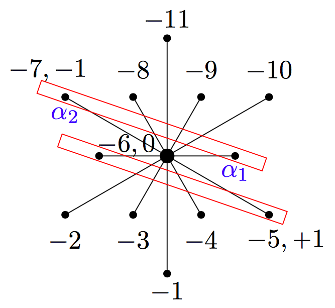
Figure 1. Filtration degrees associated with the $G_{2}$-model

We now use all of this to describe the curvature of the associated canonical Cartan geometry. Recall from §1.5.15 and 1.5.16 of [5] that a homogeneous Cartan geometry $({\mathcal{G}}\to{\mathcal{E}},\omega)$ of type $(G,P)$ over a homogeneous base manifold ${\mathcal{E}}\cong S/S^{0}$ is completely determined by a linear map $\alpha:{\mathfrak{s}}\to{\mathfrak{g}}$ that: (i) restricts to the derivative of the natural inclusion $\iota:S^{0}\to P$ on ${\mathfrak{s}}^{0}$, (ii) is $S^{0}$-equivariant, i.e. ${\rm Ad}_{\iota(s)}\circ\alpha=\alpha\circ{\rm Ad}_{s}$ for $s\in S^{0}$, and (iii) induces a vector space isomorphism ${\mathfrak{s}}/{\mathfrak{s}}^{0}\cong{\mathfrak{g}}/{\mathfrak{p}}$. Letting $\tilde{\kappa}(x,y)=\alpha[x,y]-[\alpha(x),\alpha(y)]$, the curvature corresponds to $\kappa\in\bigwedge^{2}({\mathfrak{g}}/{\mathfrak{p}})^{*}\otimes{\mathfrak{g}}$ given by

(3.7) $$\kappa(u,v)=\tilde{\kappa}(\alpha^{-1}(u),\alpha^{-1}(v)).$$

Given the $\mathfrak{sl}_{2}$-decomposition ${\mathfrak{s}}=\mathfrak{sl}_{2}\oplus V_{n}$, define $\alpha:{\mathfrak{s}}\hookrightarrow{\mathfrak{g}}=\mathfrak{gl}_{2}\oplus V_{n}={\mathfrak{q}}\oplus{\mathfrak{a}}$ via the natural inclusion. This satisfies the required conditions above, but is moreover $\mathfrak{sl}_{2}$-equivariant. This immediately implies that $\kappa$ given in (3.7) vanishes upon insertion of $\mathsf{X}\,\,{\rm mod}\ {\mathfrak{p}}$, i.e. it is of the form $\left(\begin{smallmatrix}0\\ \kappa_{2}\end{smallmatrix}\right)$.

We first check that $\kappa$ is normal. Since $\alpha$ is $\mathfrak{sl}_{2}$-equivariant, then $\kappa$ can be viewed as an $\mathfrak{sl}_{2}$-invariant element of the $\mathfrak{sl}_{2}$-module $\bigwedge^{2}({\mathfrak{g}}/{\mathfrak{q}})^{*}\otimes{\mathfrak{g}}\cong C^{2}({\mathfrak{a}},{\mathfrak{g}})$. From (3.3), it suffices to examine $\partial^{*}_{\mathfrak{a}}$ on this space. From Lemma 3.6, $C^{2}({\mathfrak{a}},{\mathfrak{q}})\subset\ker(\partial^{*}_{\mathfrak{a}})$ and $\mathrm{im}(\partial^{*}_{\mathfrak{a}})\subset C^{1}({\mathfrak{a}},{\mathfrak{q}})$. As $\mathfrak{sl}_{2}$-modules, $C^{1}({\mathfrak{a}},{\mathfrak{q}})\cong V_{n}\otimes(V_{2}\oplus V_{0})\cong V_{n+2}\oplus 2V_{n}\oplus V_{n-2}$, which contains no trivial summands for $n\geq 3$. By $\mathfrak{sl}_{2}$-equivariance of $\partial^{*}_{\mathfrak{a}}$, we conclude that $\partial^{*}\kappa=0$, i.e. $\kappa$ is normal.

A simple check using root diagrams shows that for all three cases $\kappa$ is regular and satisfies the stronger regularity condition from Remark 2.3 in the $A_{2}$ and $C_{2}$ cases. Thus, in these cases we have constructed the curvature of the canonical Cartan connection of an ODE, so these ODE are indeed of C-class. Note that in the $A_{2}$ case, there is a unique trivial summand appearing in $\bigwedge^{2}V_{4}\otimes V_{4}$, so $\kappa$ necessarily lies here. In the $C_{2}$ case, there are two trivial summands: one occurs in $\bigwedge^{2}V_{6}\otimes V_{6}$ and the other occurs inside $\bigwedge^{2}V_{6}\otimes\mathfrak{sl}_{2}$. A direct computation shows that $\kappa$ lies in their sum, but not entirely in one summand or the other.

In the $G_{2}$ case, $\kappa$ is not strongly regular. The root spaces ${\mathfrak{s}}_{\alpha_{1}+\alpha_{2}}$ and ${\mathfrak{s}}_{2\alpha_{1}+\alpha_{2}}$ have filtration degrees $-8$ and $-9$ respectively, but these insert into $\tilde{\kappa}$ to produce a nontrivial element of ${\mathfrak{s}}_{3\alpha_{1}+2\alpha_{2}}$, which has degree $-11$. Consequently, no corresponding $G_{2}$-invariant 11th order ODE exists. We have constructed a non-ODE $G_{2}$-invariant filtered $G_{0}$-structure (with symbol algebra ${\mathfrak{m}}$). Passing to the leaf space of the foliation by $E$, we obtain a $G_{2}$-invariant $\text{GL}_{2}$-structure on an 11-manifold.

4. Wilczynski–flatness and the main result

As we have observed in the end of §3.3, we can associate a canonical normal Cartan geometry to any scalar ODE of order at least $4$ and each system of ODE of order at least $3$. Using the facts on the normalization condition derived in §3, we can now express the Wilczynski invariants in terms of the curvature $\kappa$ of this Cartan geometry. We can then prove our main result that in the case of vanishing Wilczynski invariants, the normal Cartan geometry descends to the space of solutions, thus exhibiting Wilczynski–flat equations as forming a C-class.

4.1. Wilczynski invariants

Normality implies that $\kappa$ takes values in the subspace $\ker(\partial^{*})\subset L(\bigwedge^{2}({\mathfrak{g}}/{\mathfrak{p}}),{\mathfrak{g}})$. The element $\mathsf{X}\in{\mathfrak{g}}_{-}$ spans a one–dimensional $P$–invariant subspace in ${\mathfrak{g}}/{\mathfrak{p}}$. From Definition 2.4, the C-class property is confirmed if $\kappa$ takes values in the $P$-submodule

(4.1) $${\mathbb{E}}:=\{\phi\in\ker(\partial^{*})\subset C^{2}_{\operatorname{hor}}({\mathfrak{g}},{\mathfrak{g}}):i_{\mathsf{X}}\phi=0\}.$$

In terms of the vector notation introduced in §3.3, this corresponds to vectors with vanishing top component.

Composing the natural surjection $\ker(\partial^{*})\to\ker(\partial^{*})/\mathrm{im}(\partial^{*})$ with $\kappa$, we obtain the essential curvature $\kappa_{e}$ of the geometry, which is shown to be a fundamental invariant in Proposition 4.6 of [4]. From Corollary 3.8, we know that this quotient representation is completely reducible, which shows that $\kappa_{e}$ is a much simpler geometric object than $\kappa$.

To describe the relation to the generalized Wilczynski invariants, we need some preparation. Inserting the vector $\mathsf{X}$ into the curvature function $\kappa$, we obtain a function with values in $L({\mathfrak{g}}/{\mathfrak{p}},{\mathfrak{g}})$. By skew symmetry of $\kappa$, the values vanish upon insertion of $\mathsf{X}$ and thus descend to $L({\mathfrak{g}}/{\mathfrak{q}},{\mathfrak{g}})$ and one can further project to $L({\mathfrak{g}}/{\mathfrak{q}},{\mathfrak{g}}/{\mathfrak{q}})$. Now ${\mathfrak{g}}={\mathfrak{q}}\oplus{\mathfrak{a}}$ and decomposing $L({\mathfrak{g}},{\mathfrak{g}})$ accordingly, the result of that projection can be identified with the component of $\kappa(\mathsf{X},\_)$ in $L({\mathfrak{a}},{\mathfrak{a}})$.

Now ${\mathfrak{a}}$ is a representation of ${\mathfrak{q}}$, so we get ${\mathfrak{q}}\subset L({\mathfrak{a}},{\mathfrak{a}})$. In particular $\mathsf{Y}$ and, more generally, $(\mathsf{Y},A)$ for any $A\in\mathfrak{gl}_{m}$, can be viewed as an element of $L({\mathfrak{a}},{\mathfrak{a}})$. Forming powers of the map induced by $\mathsf{Y}$, we also get $(\mathsf{Y}^{k},A)\in L({\mathfrak{a}},{\mathfrak{a}})$ for $k=2,\dots,n$ and $A\in\mathfrak{gl}_{m}$. The maps $\mathsf{Y}^{k}$ for $k=1,\dots,n$ are linearly independent, and we will show that the component of $\kappa(\mathsf{X},\_)$ in $L({\mathfrak{a}},{\mathfrak{a}})$ actually has values in the subspace spanned by ${\mathfrak{q}}$ and the maps $(\mathsf{Y}^{k},A)$. Hence for each $k=1,\dots,n$, we get a well defined component of the curvature function determined by $\omega^{\mathsf{X}}\otimes\mathsf{Y}^{k}$ with values in $\mathfrak{gl}_{m}$. We will also show that the relevant components survive the projection to $\ker(\partial^{*})/\mathrm{im}(\partial^{*})$ so they are also components of the essential curvature function.

Theorem 4.1.

For a scalar ODE of order at least $4$ and systems of ODEs of order at least $3$, the generalized Wilczynski invariants from Definition 1.1 are equivalently encoded as components of the essential curvature function of the associated canonical Cartan geometry:

• $\omega^{\mathsf{X}}\otimes\mathsf{Y}^{k}$ for $k=2,\dots,n$ in case of a scalar ODE or systems of ODEs of order $n+1$;

• additionally, the trace-free part of the component corresponding to $\omega^{\mathsf{X}}\otimes\mathsf{Y}$ in case of a system of ODEs.

Vanishing of all generalized Wilczynski invariants is equivalent to the fact that the curvature function $\kappa$ has values in the sum ${\mathbb{E}}+\mathrm{im}(\partial^{*})^{1}$, where the superscript means (filtration) homogeneity $\geq 1$.

Proof.

The key ingredient for this result is the description of Wilczynski invariants in terms of a partial connection form from [10]. Given the manifold ${\mathcal{E}}$ describing the equation and the subbundle $E\subset T{\mathcal{E}}$ from §2.1, we can form the quotient bundle $N:=T{\mathcal{E}}/E$. Given sections $\xi$ of $E$ and $s$ of $N$, we can choose $\eta\in{\mathfrak{X}}({\mathcal{E}})$ which projects onto $s$, and project the Lie bracket $[\xi,\eta]$ to $N$. One immediately verifies that this gives rise to a well defined bilinear operation $D:\Gamma(E)\times\Gamma(N)\to\Gamma(N)$ which defines a partial connection, i.e. it is linear over smooth functions in the first variable and satisfies a Leibniz rule in the second variable. Hence, we write it as $(\xi,s)\mapsto D_{\xi}s$.

Now the canonical Cartan geometry gives rise to a specific description of this operation. Denoting by $p:{\mathcal{G}}\to{\mathcal{E}}$ the Cartan bundle and by $\omega$ the Cartan connection, we get $T{\mathcal{E}}={\mathcal{G}}\times_{P}({\mathfrak{g}}/{\mathfrak{p}})$, with $E\subset T{\mathcal{E}}$ corresponding to the submodule in ${\mathfrak{g}}/{\mathfrak{p}}$ spanned by $\mathsf{X}+{\mathfrak{p}}$. This module is ${\mathfrak{q}}/{\mathfrak{p}}$, so $N={\mathcal{G}}\times_{P}({\mathfrak{g}}/{\mathfrak{q}})$. Otherwise put, the bundle ${\mathcal{G}}\to{\mathcal{E}}$ defines a reduction to the structure group $P$ of the (frame bundle of the) vector bundle $N\to{\mathcal{E}}$, and we can describe the partial connection in terms of this reduction.

First, given a section $s\in\Gamma(N)$ and a lift $\eta\in{\mathfrak{X}}({\mathcal{E}})$ as above, we can further lift $\eta$ to a $P$–invariant vector field $\tilde{\eta}\in{\mathfrak{X}}({\mathcal{G}})$. Then by construction, the $P$–equivariant function ${\mathcal{G}}\to{\mathfrak{g}}/{\mathfrak{q}}$ corresponding to $s$ is given by $\omega(\tilde{\eta})+{\mathfrak{q}}$. To describe the partial connection, take $\xi\in\Gamma(E)$ and choose a $P$–invariant lift $\tilde{\xi}\in{\mathfrak{X}}({\mathcal{G}})$. Then the Lie bracket $[\tilde{\xi},\tilde{\eta}]$ is a $P$–invariant lift of $[\xi,\eta]$, so $\omega([\tilde{\xi},\tilde{\eta}])+{\mathfrak{q}}$ is the $P$–equivariant function corresponding to the projection of $[\xi,\eta]$ and thus to $D_{\xi}s$.

Since $\omega(\tilde{\xi})$ is ${\mathfrak{q}}$-valued, then by (2.6), we have

(4.2) $$\omega([\tilde{\xi},\tilde{\eta}])+{\mathfrak{q}}=-\kappa(\omega(\tilde{\xi}),\omega(\tilde{\eta}))+\tilde{\xi}\cdot\omega(\tilde{\eta})+[\omega(\tilde{\xi}),\omega(\tilde{\eta})]+{\mathfrak{q}}.$$

Let us write $f:=\omega(\tilde{\eta})+{\mathfrak{q}}$ for the function corresponding to $s$. The expression

(4.3) $$\tau(\tilde{\xi})(A+{\mathfrak{q}})=-\kappa(\omega(\tilde{\xi}),A)+[\omega(\tilde{\xi}),A]+{\mathfrak{q}}$$

is well-defined since $\omega(\tilde{\xi})$ has values in ${\mathfrak{q}}$. Thus we get a partially-defined one–form on ${\mathcal{G}}$ with values in $L({\mathfrak{g}}/{\mathfrak{q}},{\mathfrak{g}}/{\mathfrak{q}})$ (which is only defined on tangent vectors projecting to $E\subset T{\mathcal{E}}$). In terms of this form, the right hand side of (4.2) reads as $\tilde{\xi}\cdot f+\tau(\tilde{\xi})(f)$, so $\tau$ is exactly the (partial) connection form for $D$ on ${\mathcal{G}}$.

Now an interpretation of the Wilczynski invariants from [10] is based on a proof that structure group of $N$ can be reduced to $P$ in such a way that one obtains a connection form for $D$ that satisfies a normalization condition. This condition is that its values lie in the linear subspace of $L({\mathfrak{g}}/{\mathfrak{q}},{\mathfrak{g}}/{\mathfrak{q}})\cong{\mathfrak{a}}^{*}\otimes{\mathfrak{a}}$ spanned by ${\mathfrak{q}}$ and the maps of the form $(\mathsf{Y}^{2},A_{2}),\dots,(\mathsf{Y}^{n},A_{n})$ with $A_{i}\in\mathfrak{gl}_{m}$. It is then shown in [10] that the components as listed in the Theorem exactly encode the Wilczynski invariants.

To see that $\tau$ satisfies this normalization condition, observe first that $\omega(\tilde{\xi})$ has values in $\mathbb{R}\mathsf{X}\subset{\mathfrak{q}}$, so it suffices to deal with the case that $\omega(\tilde{\xi})=\mathsf{X}$. Also, the bracket–term in (4.3) gives a contribution in ${\mathfrak{q}}\subset{\mathfrak{a}}^{*}\otimes{\mathfrak{a}}$. Using the vector notation $\binom{\kappa_{1}}{\kappa_{2}}$ from §3.4 for (the values of) $\kappa$, we get $\kappa(\mathsf{X},\_)=\kappa_{1}$. The values of $\kappa_{1}$ lie in $C^{1}({\mathfrak{a}},{\mathfrak{g}})$, which as we know admits a ${\mathfrak{q}}$–invariant decomposition as $C^{1}({\mathfrak{a}},{\mathfrak{q}})\oplus C^{1}({\mathfrak{a}},{\mathfrak{a}})$. Since in (4.3) we work modulo ${\mathfrak{q}}$, the component of $\kappa$ showing up there is a multiple of the component $\kappa_{1}^{{\mathfrak{a}}}$ of $\kappa_{1}$ in $C^{1}({\mathfrak{a}},{\mathfrak{a}})$. But by Proposition 3.7, normality of $\kappa$ implies that $\kappa_{1}$ has values in $\ker(\partial^{*}_{{\mathfrak{a}}})$, while $\mathsf{Y}\cdot\kappa_{1}$ has values in $\mathrm{im}(\partial^{*}_{{\mathfrak{a}}})$. By Lemma 3.6, this means that $\kappa_{1}^{{\mathfrak{a}}}\in{\mathfrak{q}}^{\perp}\subset{\mathfrak{a}}^{*}\otimes{\mathfrak{a}}$ and that $\mathsf{Y}\cdot\kappa_{1}^{{\mathfrak{a}}}=0$. This exactly means that the values of $\kappa_{1}^{{\mathfrak{a}}}$ lie in the sum of all those lowest weight spaces of the $\mathfrak{sl}_{2}$–representation ${\mathfrak{a}}^{*}\otimes{\mathfrak{a}}$, which are perpendicular to the submodule ${\mathfrak{q}}$. These lowest weight spaces are spanned by the maps $(\mathsf{Y},A_{1}),(\mathsf{Y}^{2},A_{2}),\dots,(\mathsf{Y}^{n},A_{n})$ with $A_{1}\in\mathfrak{sl}_{m}$ and $A_{k}\in\mathfrak{gl}_{m}$ for $k=2,\dots,n$.

Thus we conclude that $\tau$ satisfies the normalization condition and that the Wilczynski invariants are equivalently encoded by the class of $\kappa(\mathsf{X},\_)$ modulo $C^{1}({\mathfrak{a}},{\mathfrak{q}})$. In particular, this class and thus $\kappa_{1}^{{\mathfrak{a}}}$ vanishes identically in the Wilczynski–flat case.

Having all that in hand, the claims in the theorem now follow from two simple observations. On the one hand, Proposition 3.7 and Lemma 3.6 show that the restriction of the $P$–equivariant map $\phi=\binom{\phi_{1}}{\phi_{2}}\mapsto\phi_{1}^{{\mathfrak{a}}}$ to $\ker(\partial^{*})\subset C^{2}_{\operatorname{hor}}({\mathfrak{g}},{\mathfrak{g}})$ vanishes on the subspace $\mathrm{im}(\partial^{*})$. Thus it factorizes to the quotient $\ker(\partial^{*})/\mathrm{im}(\partial^{*})$, which shows that $\kappa_{1}^{{\mathfrak{a}}}$ and thus the components encoding the Wilczynski invariants are components of the essential curvature function $\kappa_{e}$. This also shows that if $\kappa$ has values in $\mathbb{E}+\mathrm{im}(\partial^{*})^{1}$, then $\kappa_{e}$ vanishes upon insertion of $\mathsf{X}$ and hence all Wilczynski invariants vanish.

On the other hand, suppose that we start from a Wilczynski–flat equation, so $\kappa=\binom{\kappa_{1}}{\kappa_{2}}\in\ker(\partial^{*})$ has the property that $\kappa_{1}^{{\mathfrak{a}}}=0$. Then by Lemma 3.6, $\kappa_{1}=\kappa_{1}^{\mathfrak{q}}\in\mathrm{im}(\partial^{*}_{\mathfrak{a}})$, so we can take an element $\psi_{1}\in C^{2}({\mathfrak{a}},{\mathfrak{g}})$ such that $\partial^{*}_{\mathfrak{a}}\psi_{1}=-\kappa_{1}$. Compatibility with homogeneities shows that we may assume that $\psi_{1}$ is homogeneous of degree $\geq 0$. But then by Proposition 3.7, $\binom{\kappa_{1}}{\kappa_{2}}-\partial^{*}\binom{\psi_{1}}{0}$ has vanishing top–component and thus lies in ${\mathbb{E}}$. Hence, $\binom{\kappa_{1}}{\kappa_{2}}\in{\mathbb{E}}+\mathrm{im}(\partial^{*})^{1}$, which completes the proof. ∎

4.2. The covariant exterior derivative

Let $({\mathcal{G}}\to M,\omega)$ be a regular Cartan geometry of type $({\mathfrak{g}},P)$. Following [4], we consider the operator $d^{\omega}:\Omega^{k}({\mathcal{G}},{\mathfrak{g}})\to\Omega^{k+1}({\mathcal{G}},{\mathfrak{g}})$ defined by

$$(d^{\omega}\varphi)(\xi_{0},...,\xi_{k})=d\varphi(\xi_{0},...,\xi_{k})+\textstyle\sum_{i=0}^{k}(-1)^{i}[\omega(\xi_{i}),\varphi(\xi_{0},...,\widehat{\xi_{i}},...,\xi_{k})],$$

where $\xi_{j}\in{\mathfrak{X}}({\mathcal{G}})$ for all $j$. By Proposition 4.2 of [4], if $\varphi$ is horizontal and $P$–equivariant, then so is $d^{\omega}\varphi$. Moreover, $d^{\omega}$ is compatible with the natural notion of homogeneity for ${\mathfrak{g}}$–valued differential forms, and the curvature $K$ of $\omega$ satisfies the Bianchi identity $d^{\omega}K=0$.

4.3. Wilczynski-flat ODE are of C-class

Now we are ready to prove our main result.

Theorem 4.2.

Any Wilczynski-flat ODE (1.1) with $m=1$, $n\geq 3$ or $m\geq 2$, $n\geq 2$ is of C-class.

Proof.

Let $({\mathcal{G}}\to{\mathcal{E}},\omega)$ be the regular, normal Cartan geometry of type $({\mathfrak{g}},P)$ associated to (1.1) as in Theorem 2.2. We have to show that for a Wilczynski–flat ODE, the curvature function $\kappa$ has values in the module ${\mathbb{E}}$ defined in (4.1). Generalizing the relation between the curvature $K$ and the curvature function $\kappa$, horizontal ${\mathfrak{g}}$–valued $k$–forms on ${\mathcal{G}}$ can be naturally identified with smooth functions ${\mathcal{G}}\to L(\bigwedge^{k}({\mathfrak{g}}/{\mathfrak{p}}),{\mathfrak{g}})$. The natural notions of $P$–equivariance in the two pictures correspond to each other, see Theorem 4.4 of [4]. For the current proof, it will be helpful to switch between forms and equivariant functions freely, so we will express the fact that $\kappa$ has values in ${\mathbb{E}}$ as “$K$ lies in ${\mathbb{E}}$”. In these terms, composing functions with $\partial^{*}$ defines a tensorial operator $\Omega^{k}_{\operatorname{hor}}({\mathcal{G}},{\mathfrak{g}})\to\Omega^{k-1}_{\operatorname{hor}}({\mathcal{G}},{\mathfrak{g}})$ for each $k$, and we also denote this operator by $\partial^{*}$. By construction, $\partial^{*}$ maps $P$–equivariant forms to $P$–equivariant forms. In this language, normality can be simply expressed as $\partial^{*}K=0$.

By Theorem 4.1, Wilczynski–flatness implies that $K$ has values in ${\mathbb{E}}+\mathrm{im}(\partial^{*})^{1}$. Passing to equivariant functions, applying Lemma 4.7 of [4], and passing back to differential forms, we conclude that $K=K_{1}+K_{2}$ for $P$–equivariant forms $K_{1},K_{2}\in\Omega^{2}_{\operatorname{hor}}({\mathcal{G}},{\mathfrak{g}})$ such that $K_{1}$ has values in ${\mathbb{E}}$ and $K_{2}$ has values in $\mathrm{im}(\partial^{*})^{1}$. Now we prove the theorem in a recursive way by showing that for any $\ell\geq 1$, from a decomposition $K=K_{1}+K_{2}$ such that $K_{1}$ has values in ${\mathbb{E}}$ and $K_{2}$ has values in $\mathrm{im}(\partial^{*})^{\ell}$, we can always obtain a decomposition $K=\tilde{K}_{1}+\tilde{K}_{2}$, for which $\tilde{K}_{1}$ again has values in ${\mathbb{E}}$ but $\tilde{K}_{2}$ has values in $\mathrm{im}(\partial^{*})^{\ell+1}$. Since $\mathrm{im}(\partial^{*})^{r}=\{0\}$ for sufficiently large $r$, this implies the result.

So let us assume that $K=K_{1}+K_{2}$ as above with $K_{2}$ having values in $\mathrm{im}(\partial^{*})^{\ell}$ for some $\ell\geq 1$. We first claim that for a $P$–equivariant form $\varphi\in\Omega^{2}_{\operatorname{hor}}({\mathcal{G}},{\mathfrak{g}})$, which has values in ${\mathbb{E}}$, also $\partial^{*}d^{\omega}\varphi$ has values in ${\mathbb{E}}$. In terms of the description of $\partial^{*}$ from Proposition 3.7, lying in ${\mathbb{E}}$ means that the top component of the right hand side of (3.3) has to vanish. Denoting by $\hat{X}\in{\mathfrak{X}}({\mathcal{G}})$ the vector field characterized by $\omega(\hat{X})=\mathsf{X}$, we thus have to show that (the equivariant function corresponding to) $i_{\hat{X}}d^{\omega}\varphi$ has values in $\ker(\partial^{*}_{\mathfrak{a}})\subset C^{2}({\mathfrak{a}},{\mathfrak{g}})$.

The assumption on $\varphi$ implies $i_{\hat{X}}\varphi=0$, so for vector fields $\xi,\eta\in{\mathfrak{X}}({\mathcal{G}})$, we get

(4.4) $$(i_{\hat{X}}d^{\omega}\varphi)(\xi,\eta)=d\varphi(\hat{X},\xi,\eta)+[X,\varphi(\xi,\eta)].$$

Using $i_{\hat{X}}\varphi=0$ once more, we get

(4.5) $$d\varphi (\hat{X},\xi,\eta)=\hat{X}\cdot\varphi(\xi,\eta)-\varphi([\hat{X},\xi],\eta)-\varphi(\xi,[\hat{X},\eta])=$$

$$\hat{X}\cdot f(\omega(\xi),\omega(\eta))-f(\omega([\hat{X},\xi]),\omega(\eta))-f(\omega(\xi),\omega([\hat{X},\eta])).$$

Here $f$ denotes the equivariant function corresponding to $\varphi$, which takes values in ${\mathbb{E}}\subset\ker(\partial^{*})$. By Proposition 3.7, $f$ in fact has values in $\ker(\partial^{*}_{{\mathfrak{a}}})\subset C^{2}({\mathfrak{a}},{\mathfrak{g}})$. Since $\omega(\hat{X})$ is constant, then by (2.6),

(4.6) $$\omega([\hat{X},\xi])=-K(\hat{X},\xi)+[X,\omega(\xi)]+\hat{X}\cdot\omega(\xi),$$

and likewise for $\omega([\hat{X},\eta])$.

Now by assumption $K=K_{1}+K_{2}$ and $i_{\hat{X}}K_{1}=0$, so $K(\hat{X},\xi)=\kappa_{2}(\mathsf{X},\omega(\xi))$ and $\kappa_{2}$ has values in $\mathrm{im}(\partial^{*})$. By Proposition 3.7, this means that $\kappa_{2}(\mathsf{X},\_)$ has values in $\mathrm{im}(\partial^{*}_{{\mathfrak{a}}})$, which by part (3) of Lemma 3.6 is contained in ${\mathfrak{q}}$. In particular, terms of the form $K(\hat{X},\xi)$ insert trivially into $f$, so these do not contribute. On the other hand, the contribution to (4.5) resulting from the last term in (4.6) is

$$-f(\hat{X}\cdot\omega(\xi),\omega(\eta))-f(\omega(\xi),\hat{X}\cdot\omega(\eta)).$$

This adds up with the first term in the right hand side of (4.5) to $(\hat{X}\cdot f)(\omega(\xi),\omega(\eta))$. Since $f$ has values in ${\mathbb{E}}$, the derivative $\hat{X}\cdot f$ has the same property. Now inserting the last remaining term in the right hand side of (4.6) into the right hand side of (4.5), we obtain

$$-f([X,\omega(\xi)],\omega(\eta))-f(\omega(\xi),[X,\omega(\eta)]).$$

Viewing $f$ as a function with values in $\ker(\partial^{*}_{{\mathfrak{a}}})\subset C^{2}({\mathfrak{a}},{\mathfrak{g}})$ as above, we can write the sum of these terms with the last term in the right hand side of (4.4) as $(\rho_{\mathsf{X}}\circ f)(\omega(\xi),\omega(\eta))$. Here $\rho_{\mathsf{X}}$ denotes the natural action of $\mathsf{X}\in{\mathfrak{q}}$ on $C^{2}({\mathfrak{a}},{\mathfrak{g}})$. But then ${\mathfrak{q}}$–equivariance of $\partial^{*}_{{\mathfrak{a}}}$ as proved in part (1) of Lemma 3.6 shows that also this function has values in $\ker(\partial^{*}_{{\mathfrak{a}}})$, which completes the proof of the claim.

Returning to our decomposition $K=K_{1}+K_{2}$, we now use the Bianchi identity $d^{\omega}K=0$ to get $\partial^{*}d^{\omega}K_{2}=-\partial^{*}d^{\omega}K_{1}$, so by the claim, this has values in ${\mathbb{E}}$. Now consider the maps $\partial_{{\mathfrak{g}}_{-}}$ and $\underline{\partial^{*}}$ defined on the spaces $C^{k}({\mathfrak{g}}_{-},{\mathfrak{g}})$ as in the proof of Proposition 3.3, and the algebraic Laplacian $\Box:=\partial_{{\mathfrak{g}}_{-}}\circ\underline{\partial^{*}}+\underline{\partial^{*}}\circ\partial_{{\mathfrak{g}}_{-}}$, which preserves degrees and homogeneity. This clearly can be restricted to an endomorphism of $\mathrm{im}(\underline{\partial^{*}})\subset C^{2}({\mathfrak{g}}_{-},{\mathfrak{g}})_{\ell}$ (on which it coincides with $\underline{\partial^{*}}\circ\partial_{{\mathfrak{g}}_{-}}$), and in the proof of Proposition 3.10 of [4] it is shown that this restriction is bijective. By the Cayley–Hamilton theorem, there is a polynomial $p_{\ell}\in{\mathbb{R}}[x]$ such that $p_{\ell}(\Box)$ is inverse to $\Box$ on $\mathrm{im}(\underline{\partial^{*}})_{\ell}$. Now $p_{\ell}(\partial^{*}d^{\omega})$ is a well-defined operator on the space of $P$–equivariant forms in $\Omega^{2}_{\operatorname{hor}}({\mathcal{G}},{\mathfrak{g}})$, which preserves homogeneities.

Applying our claim once more, we see that $p_{\ell}(\partial^{*}d^{\omega})\partial^{*}d^{\omega}K_{2}$ has values in ${\mathbb{E}}$ and by construction is still homogeneous of degree $\geq\ell$. Thus, $\tilde{K}_{1}=K_{1}+p_{\ell}(\partial^{*}d^{\omega})\partial^{*}d^{\omega}K_{2}$ has values in ${\mathbb{E}}$, while $\tilde{K}_{2}:=K_{2}-p_{\ell}(\partial^{*}d^{\omega})\partial^{*}d^{\omega}K_{2}$ has values in $\mathrm{im}(\partial^{*})$ and is homogeneous of degree $\geq\ell$. To verify that $K=\tilde{K}_{1}+\tilde{K}_{2}$ is the desired decomposition, it suffices to show that the homogeneous component of degree $\ell$ of (the equivariant function corresponding to) $\tilde{K}_{2}$ vanishes identically.

By part (3) of Theorem 4.4 of [4], for a $P$–equivariant form $\varphi\in\Omega^{2}({\mathcal{G}},{\mathfrak{g}})$ which is homogeneous of degree $\geq\ell$ and corresponds to the equivariant function $f$, the homogeneous component of degree $\ell$ of the equivariant function corresponding to $\partial^{*}d^{\omega}\varphi$ is given by $\underline{\partial^{*}}\circ\partial_{{\mathfrak{g}}_{-}}\circ\mathrm{gr}_{\ell}\circ f$. Applying this iteratively starting with the function $\kappa_{2}$ corresponding to $K_{2}$, we remain in the realm of functions having values in $\mathrm{im}(\partial^{*})^{\ell}$. Thus we iteratively conclude that the homogeneous component of degree $\ell$ of the function corresponding to $p_{\ell}(\partial^{*}d^{\omega})\partial^{*}d^{\omega}K_{2}$ coincides with $p_{\ell}(\Box)\circ\Box\circ\mathrm{gr}_{\ell}\circ\kappa_{2}=\mathrm{gr}_{\ell}\circ\kappa_{2}$, which shows that $\tilde{K}_{2}$ has vanishing homogeneous component of degree $\ell$. ∎

Example 4.3.

Let ${\mathbf{u}}=(u^{1},...,u^{m})$. The equations for circles in an $(m+1)$-dimensional Euclidean space are given by

$${\mathbf{u}}^{\prime\prime\prime}=3{\mathbf{u}}^{\prime\prime}\frac{\langle{\mathbf{u}}^{\prime},{\mathbf{u}}^{\prime\prime}\rangle}{1+\langle{\mathbf{u}}^{\prime},{\mathbf{u}}^{\prime}\rangle}.$$

This ODE system is conformally invariant, and it has been verified that the Wilczynski invariants vanish [22, Prop.2]. By our Theorem 4.2, the system is of C-class. For $m=1$, the equation is (contact) trivializable, but for $m\geq 2$ the system is not (point) trivializable.

Since the Wilczynski invariants for linear equations are invariants, it follows that an ODE with trivializable linearizations is Wilczynski–flat. Hence we obtain

Corollary 4.4.

Let $n\geq 2$, $m\geq 1$, with $(n,m)\neq(2,1)$. Any ODE (1.1) for which the linearization around any solution is trivializable, is of C-class.

Example 4.5.

The ODE $u^{(n+1)}-\frac{n+1}{n}\frac{(u^{(n)})^{2}}{u^{(n-1)}}=0$, for $n\geq 3$, is submaximally symmetric [25, p.206] except when $n=4$ and $6$. At a fixed solution $u$, its linearization is the ODE for $v$ given by

(4.7) $$\ell_{u}[v]:=v^{(n+1)}-\frac{2(n+1)}{n}av^{(n)}-\frac{n+1}{n}a^{2}v^{(n-1)}=0,$$

where $a:=\frac{u^{(n)}}{u^{(n-1)}}$. We have $a^{\prime}=\frac{a^{2}}{n}$ and hence $(\frac{1}{a})^{\prime}=-\frac{1}{n}$, $(\frac{1}{a^{2}})^{\prime}=-\frac{2}{na}$ and $(\frac{1}{a^{2}})^{\prime\prime}=\frac{2}{n^{2}}$. Defining $\tilde{v}=\frac{v}{a^{2}}$, we have $\tilde{v}^{(n+1)}=\frac{1}{a^{2}}\ell_{u}[v]=0$, so (4.7) is trivializable, and the given ODE is of C-class by Corollary 4.4. This example is included into a larger family of Wilczynski-flat (hence C-class) equations given in [10, Example 2].

Example 4.6.

Let $m\geq 2$ and $n\geq 2$. Given ${\mathbf{u}}=(u^{1},...,u^{m})$, consider

$${\mathbf{u}}^{(n+1)}=\mathbf{f},\quad\mbox{where}\quad f_{i}=\begin{cases}0,&i\neq m;\\ ((u^{1})^{(n)})^{2},&i=m.\end{cases}$$

Its linearization is easily seen to be trivializable, so it is of C-class. It is not trivializable since a fundamental invariant does not vanish on it, namely $I_{2}$ in [12]. A similar 2nd order example was given in [20, (5.6a)], which was known to be of C-class since it is torsion-free [17].

4.4. Remark: A potential alternative line of argument

To conclude the article, let us briefly outline how the theory we have developed could be used to obtain an alternative proof of our main result. This line of argument is based on correspondence spaces which are familiar in the case of parabolic geometries. It depends crucially on the existence of a natural Segré structure on the space of solutions of a Wilczynski-flat ODE from [10], compare with §2.4. As mentioned there, Segré structures are classical first order structures corresponding to $Q\subset\text{GL}({\mathfrak{a}})$. Hence such a structure on a space $S$ comes with a $Q$–principal bundle ${\mathcal{G}}\to S$. The classical way to study such structures is via the Spencer differential. As we have noted in the proof of Proposition 3.5, this coincides with the restriction of $\partial_{{\mathfrak{a}}}$ to a map $C^{1}({\mathfrak{a}},{\mathfrak{q}})\to C^{2}({\mathfrak{a}},{\mathfrak{a}})$ and is injective. Choosing a $Q$–invariant complement ${\mathcal{N}}\subset C^{2}({\mathfrak{a}},{\mathfrak{a}})$ to the image of the Spencer differential, there is a canonical principal connection form $\tau$ on ${\mathcal{G}}$ characterized by the fact that its torsion lies in ${\mathcal{G}}\times_{Q}{\mathcal{N}}\subset\bigwedge^{2}T^{*}S\otimes TS$.

Usually, not too much emphasis is put on the actual choice of ${\mathcal{N}}$, but in the case of Segré structures, this is a surprisingly subtle issue. Analyzing $\partial_{\mathfrak{a}}:{\mathfrak{a}}^{*}\otimes{\mathfrak{q}}\to\bigwedge^{2}{\mathfrak{a}}^{*}\otimes{\mathfrak{a}}$ in terms of representations of ${\mathfrak{q}}$, one easily deduces that there always exist $Q$–invariant complements, but aside from the $(m,n)=(1,3)$ case, there is always a freedom of choice. The larger $m$ and $n$ get, the bigger this freedom becomes, and while there are always only finitely many free parameters involved, their number gets arbitrarily high.

Now it turns out that the construction from §3.2 can also be used to construct uniform normalization conditions for Segré structures. Indeed, we can view $L(\bigwedge^{2}({\mathfrak{g}}/{\mathfrak{q}}),{\mathfrak{g}})$ as the subspace in $C^{2}({\mathfrak{g}},{\mathfrak{g}})$ consisting of all cochains vanishing upon insertion of one element of ${\mathfrak{q}}$. Similarly as in Lemma 3.2 one shows that this subspace is preserved by $\partial^{*}$ and that the restriction of $\partial^{*}$ to it is $Q$–equivariant. Using a similar adjointness result as in Proposition 3.3, one shows that ${\mathcal{N}}:=\ker(\partial^{*}_{\mathfrak{a}})\subset C^{2}({\mathfrak{a}},{\mathfrak{a}})$ is a $Q$–invariant complement to the image of the Spencer differential.

Now the alternative approach for proving that Wilczynski–flat ODE form a C-class goes as follows. Starting with such an ODE ${\mathcal{E}}$, form a local space ${\mathcal{S}}$ of solutions. As proved in [10], this space of solutions inherits a natural Segré structure. This gives rise to a principal $Q$–bundle ${\mathcal{G}}\to{\mathcal{S}}$, which we may endow with the canonical principal connection $\tau\in\Omega^{1}({\mathcal{G}},{\mathfrak{q}})$ for the choice ${\mathcal{N}}:=\ker(\partial^{*}_{\mathfrak{a}})$ of normalization condition. Taking the canonical soldering form $\theta$ on ${\mathcal{G}}$, which can be viewed as having values in ${\mathfrak{a}}$, we can form $\theta\oplus\tau$, and this defines a Cartan connection $\omega$ of type $({\mathfrak{g}},Q)$ on ${\mathcal{G}}$.

The restriction of the principal action of $Q$ defines a free right action of $P\subset Q$ on ${\mathcal{G}}$, and we can form the correspondence space, i.e. the space ${\mathcal{C}}{\mathcal{S}}:={\mathcal{G}}/P$ of orbits. This can be identified with the total space of the associated bundle ${\mathcal{G}}\times_{Q}(Q/P)$. Of course, ${\mathcal{G}}\to{\mathcal{C}}{\mathcal{S}}$ is a principal $P$–bundle and it is easy to verify that $\omega$ also is a Cartan connection of type $({\mathfrak{g}},P)$ on ${\mathcal{G}}\to{\mathcal{C}}{\mathcal{S}}$.

Guided by what happens for parabolic geometries, we expect that it is possible to show that ${\mathcal{C}}{\mathcal{S}}$ is locally isomorphic to ${\mathcal{E}}$, so $({\mathcal{G}},\omega)$ can be locally viewed as a Cartan geometry of type $({\mathfrak{g}},P)$ over ${\mathcal{E}}$. This isomorphism is expected to have the property that the underlying filtered $G_{0}$–structure of this Cartan geometry is the given structure on ${\mathcal{E}}$. From our choice of normalization conditions it follows that $\omega$ is also normal (in the sense used in this article) as a Cartan connection of type $({\mathfrak{g}},P)$. Uniqueness of the normal Cartan geometry implies that $({\mathcal{G}},\omega)$ is locally isomorphic to the canonical Cartan geometry on ${\mathcal{E}}$ and by construction it descends to the local space ${\mathcal{S}}$ of solutions, which would complete the argument.

References

- [1] R. Bryant, Two exotic holonomies in dimension four, path geometries, and twistor theory, Proc. Symp. Pure Math. 53 (1991), 33–88.
- [2] D.M.J. Calderbank, T. Diemer, Differential invariants and curved Bernstein–Gelfand–Gelfand sequences, J. reine angew. Math. 537 (2001), 67–103.
- [3] A. Čap, Correspondence spaces and twistor spaces for parabolic geometries, J. Reine Angew. Math. 582 (2005), 143–172.
- [4] A. Čap, On canonical Cartan connections associated to filtered G-structures, preprint arXiv:1707.05627 (2017).
- [5] A. Čap, J. Slovák, Parabolic Geometries I: Background and General Theory, American Mathematical Society, 2009.
- [6] A. Čap, J. Slovák, V. Souček, Bernstein–Gelfand–Gelfand sequences, Ann. Math. 154 (2001), 97–113.
- [7] A. Čap, V. Souček, Relative BGG sequences; II. BGG machinery and invariant operators, Adv. Math. 320 (2017) 1009–1062.
- [8] É. Cartan, Les espaces généralisés et l’intégration de certaines classes d’équations différentielles, C.R., 1938, V.206, N.23, 1689–1693.
- [9] B. Doubrov, Contact trivialization of ordinary differential equations, Differential geometry and its applications. Proceedings of the 8th international conference, Opava, Czech Republic, August 27–31, 2001. Math. Publ. (Opava) 3 (2001), pp. 73–84.
- [10] B. Doubrov, Generalized Wilczynski invariants for nonlinear ordinary differential equations, The IMA Volumes in Mathematics and its Applications 144 (2008), 25–40.
- [11] B. Doubrov, B. Komrakov, T. Morimoto, Equivalence of holonomic differential equations, Lobachevskij Journal of Mathematics 3 (1999), 39–71.
- [12] B. Doubrov, A. Medvedev, Fundamental invariants of systems of ODEs of higher order. Differential Geom. Appl. 35 (2014), suppl., 291–313.
- [13] M. Dunajski, M. Godliński, structures, geometry and twistor theory, Q. J. Math. 63(2012), no. 1, 101–132.
- [14] M. Dunajski, P. Tod, Paraconformal geometry of -th order ODEs, and exotic holonomy in dimension four, J. Geom. Phys. 56 (2006) 1790–1809.
- [15] M.E. Fels, The equivalence problem for systems of second-order ordinary differential equations, Proc. London Math. Soc. (3) 71 (1995), 221–240.
- [16] M. Godlinski, P. Nurowski, geometry of ODE’s, J. Geom. Phys. 60 (2010), no. 6-8, 991–1027.
- [17] D. Grossman, Torsion-free path geometries and integrable second order ODE systems, Selecta Math. 6, no. 4 (2000), 399–442.
- [18] S. Kobayashi, T. Nagano, On filtered Lie algebras and geometric structures. I. J. Math. Mech. 13 (1964), 875–907.
- [19] S. Kobayashi, T. Nagano, On filtered Lie algebras and geometric structures. III. J. Math. Mech. 14 (1965), 679–706.
- [20] B. Kruglikov, D. The, The gap phenomenon in parabolic geometries. J. Reine Angew. Math. 2017(723), 153–215 (2014).
- [21] W. Kryński, Paraconformal structures and differential equations. Differential Geom. Appl. 28 (2010), no. 5, 523–531.
- [22] A. Medvedev, Third order ODEs systems and its characteristic connections, SIGMA 7 (2011), Paper 076, 15 pp.
- [23] T. Morimoto, Geometric structures on filtered manifolds, Hokkaido Math. J. 22 (1993), 263–347.
- [24] P. Nurowski, Comment on geometry of fourth-order ODEs, J. Geom. Phys. 59 (2009), no. 3, 267–278.
- [25] P.J. Olver, Equivalence, Invariants and Symmetry, Cambridge University Press, 1995.
- [26] Y. Se-ashi, On differential invariants of integrable finite type linear differential equations, Hokkaido Math. J. 17 (1988), 151–195.
- [27] N. Tanaka, K. Kiyohara, T. Morimoto, K. Yamaguchi, Geometric Theory of Systems of Ordinary Differential Equations I, Hokkaido University Technical Report Series in Mathematics, no. 169, March 2017, 1–169. http://doi.org/10.14943/81531
- [28] N. Tanaka, K. Kiyohara, T. Morimoto, K. Yamaguchi, Geometric Theory of Systems of Ordinary Differential Equations II, Hokkaido University Technical Report Series in Mathematics, no. 170, March 2017. http://doi.org/10.14943/81532
- [29] E.J. Wilczynski, Projective differential geometry of curves and ruled surfaces, Leipzig, Teubner, 1905.