A Nonparametric Model for Multimodal Collaborative Activities Summarization

Abstract

Ego-centric data streams provide a unique opportunity to reason about joint behavior by pooling data across individuals. This is especially evident in urban environments teeming with human activities, but which suffer from incomplete and noisy data. Collaborative human activities exhibit common spatial, temporal, and visual characteristics facilitating inference across individuals from multiple sensory modalities as we explore in this paper from the perspective of meetings.

We propose a new Bayesian nonparametric model that enables us to efficiently pool video and GPS data towards collaborative activities analysis from multiple individuals. We demonstrate the utility of this model for inference tasks such as activity detection, classification, and summarization. We further demonstrate how spatio-temporal structure embedded in our model enables better understanding of partial and noisy observations such as localization and face detections based on social interactions. We show results on both synthetic experiments and a new dataset of egocentric video and noisy GPS data from multiple individuals.

1 Introduction

Consider individuals equipped with wearable cameras and GPS devices going about an urban center, meeting and interacting with each other. Aggregation of their ego-centric data streams leads to a richer understanding of their collaborative experience, whereas analysis of the individual streams suffers from noisy, partially denied, and unstructured signals. Here, we suggest an approach to infer collaborative activities such as “meetings” or “interactions” from streaming wearable sensors based on a collective multi-modal generative model. Inference allows us to summarize and perform analysis in the context of life-logging, detecting special events from multiple sensors, and supporting coordinated human activities. Interestingly, by combining multiple ego-centric data streams, one can infer the activities of one individual using the data of another. The underlying model handles noisy and partially denied data streamed from multiple (wearable) devices, a crucial capability in noisy sensory environments.

By treating collaborative activity instances as latent factors with a spatio-temporal structure, we can summarize activities for co-located individuals despite noisy and partial/missing signals by pooling data for the purpose of collaborative reasoning. Human observers can understand such content (at small scale) with the appropriate visualizations, partially because we understand the spatio-temporal and semantic structure of human activities. We seek to automate such abilities via an inference procedure that summarizes collective and individual experiences via the aggregated data streams.

We explore meetings between people as a case study for detecting, characterizing, and utilizing the temporal and collaborative structure of activities. We examine summarization as a task that benefits from higher-level information, even in the cases that activity detections are uncertain given the observations. Pooled information from multiple sensors (e.g., video, GPS) and multiple individuals, coupled with a structured model for activities, allows us to handle partial information in both GPS and video data and reduce the uncertainty regarding the participants across modalities. The proposed approach is robust to missing data and low-quality, poor-vantage point footage that is unsuitable for strong geometric reasoning such as 3D reconstruction. Consider, for instance, a commute via a crowded subway or a family ski trip. Such scenarios include non-rigid 3D motion, missing and noisy GPS observations [35], abrupt viewpoint changes, and video segments which lack features or textures. Yet, a casual observer of videos and GPS traces from these activities could readily piece together a common story without the need for a full model of the environment.

Contributions Here we present a model that captures these characteristics.

1. We propose a probabilistic model and inference algorithms for the explanation of egocentric video and GPS data in terms of human activities. This model allows us to handle multiple, overlapping activity definitions and partial data in all modalities, by pooling data from across individuals and modalities.

2. Using our model, we demonstrate detection and summarization of collaborative human activities from egocentric cameras and GPS signals in an urban environment where both the visual and the GPS signals are either missing or distorted.

3. We demonstrate improved localization of individuals conditioned on detected activities from corrupt and partial sources such as GPS and egocentric video streams.

4. We provide a dataset to allow further annotation and examination of similar methods, in order to foster future discussion and improvements.

Our model is derived from simple assumptions, and we show its relevance to complex tasks on multimodal data. Activities are detected through a sampling approach for the activity instances and their parameters. The model is easily extensible to other sensory modalities, such as inertial sensors [3], or textual sources [30]. We describe the assumptions and the model in Section 2, and the associated activity inference, localization, and summarization procedures in Section 3. In Section 4 we demonstrate our ability to infer the activities and leverage this analysis towards improved localization and understanding of people’s story as portrayed by the data. Section 5 discusses possible extensions and concludes the report. In Appendix A we present extensions to the social dynamic models described below. This is followed by additional details on the sampling procedure in Appendix B and a approach for video summarization based on the sampled activity instances in Appendix C.

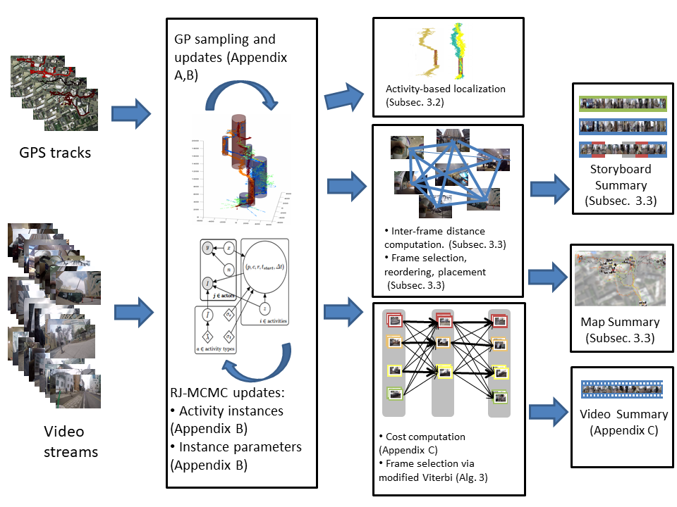
Figure 1: Our model reasons over multiple video and GPS streams, inferring and summarizing collaborative interactions. We employ a generative model utilizing Gaussian processes for GPS and learned likelihood models for the semantic visual content and recognized faces. This enables summarization of the participants experience, detection of specific activities, and correction of the individuals’ partial GPS and visual detections streams.

1.1 Related work

Our paper relates to several lines of research. These have attempted to tackle activity inference using GPS, visual, and other sensor data (for example, [21], [34, 4, 32] and [17], respectively). However, our model reasons over latent locations and activities conditioned on the set of visual and GPS cues, marginalizing over possible interpretations of the data. We do not assume that activities form partitions or hierarchies over the timeline except in specific cases, even for a single person. This is due both to a non-trivial overlap structure and to multiple, equally-plausible interpretation of the observations. Such structures lend themselves to probabilistic models that can describe multiple interpretations. For an illustration of the possible relation between different activities’ time span, consider the illustrative example in Figure 2.

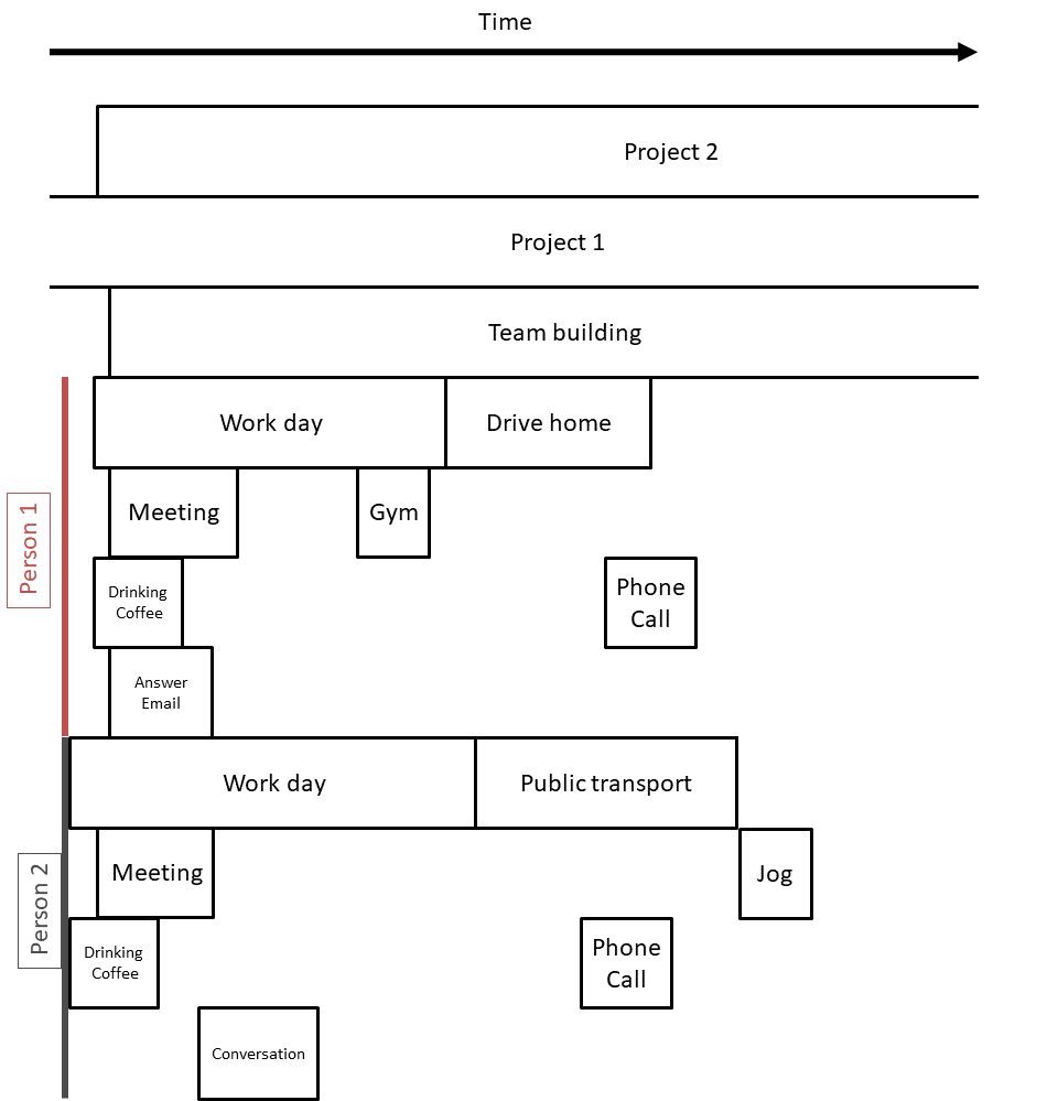
Figure 2: Time intervals for several activities in a work/office scenario involving 2 people. Note the non-hierarchical structure formed between activities even for a single person, let alone multiple participants. Some activities are best inferred via visual data (e.g. drinking coffee) while others are easily inferred via GPS (e.g., driving home), or require significant priors on human activities to infer (e.g., team building / project 1). Some activities in this figure correspond to American Time-Use Survey(ATUS)[25] Lexicon category codes such as 180501 (drive home / public transport), 050201 (phone call), 050202 (drinking coffee), 130124 (jogging), while others are higher-level (team building, project 1) or potentially lower-level.

Sampling allows us to reason about activities without committing to a single “correct” explanation. This approach of multiple explanations can be maintained, as we show, throughout the analysis while gracefully handling partial/corrupt data.

Several lines of research have explored multiple video streams for reasoning over collaborative activities. These methods generally assume that all participants observe the same scene with uninterrupted data streams [33, 8], [16, 7], or that the 3D environment can be reliably inferred [23, 2, 18]. The proposed method does not rely on such restrictive assumptions, allowing for partial, discontinuous, and noisy observations over multiple scenes amongst varying subsets of participants and eschewing reconstruction as an intermediate step altogether. The method is robust to non-rigid 3D motion and fast rotations, as well as GPS denial. Several efforts have been dedicated to meaningfully choosing which data to display and when, regarding both frame selection [8], and alignment [33, 5]. Quality measures for each shot are often used in a constrained graph traversal [36, 2]. There, activity inference is treated separately from the understanding of how different sources relate to one another. While incorporation of semantics for summarization was done, for example, by Tat-Jen et al. [28] and Lu et al. [22, 20], it was done so only at the feature level of objects/instantaneous interaction, rather than over complete activities, due to a variety of challenges including the difficulty of classifying the start and end of activities in an arbitrary video, be it egocentric or third-person. Inferring human activities from such data is non-trivial, particularly in the absence of reliable activity labelling.

2 Model

We define a collaborative activity as one in which two or more individuals, or actors (as we call them henceforth), are spatially proximate for some finite duration accompanied by distinctive categorical features. While we emphasize collaborative summarization and joint activities, the model may encompass individual activities as well. A key attribute of the model is that by integrating multiple ego-centric data streams, one can infer the activities of one actor using the data of a different actor.

We define activities as having a categorical activity type carrying some semantic meaning — in our data and prior feature distributions we exemplify “coffeeshop” vs. “chance street meeting”. We could extend to other fixed or inferred types, e.g., “work meeting” or “gym workout”. These types parameterize the prior distribution of meeting characteristics, such as spatio-temporal extent and visual content. For each activity type there may be multiple instances, or activities of that type. The $i$-th activity instance has a static center $c_{i}$ and radius $r_{i}$. A configuration is the set of all activity instances occurring and explaining the observation. Subsection 2.2 describes a probabilistic model that defines the probability of a set of observations given a configuration and its parameters. Subsequently, configurations may be sampled from this model.

Activity instances of different types may overlap in time, space, and participants depending on the activity types involved, e.g lunch may be part of a working day, but sleep and gym-practice do not overlap. The activity set of each actor is far from being a partition, as assumed in many models for activity recognition. Instead, each activity is an uncertain function of the physical/geometric scene content and participants. This view favors a nonparametric model where activity instances are random occurrences.

Here, we discuss the mathematical model by which we represent the trajectories of actors, their collaborative activities, and related visual cues. The overlap structure of different activity types is assumed to be known in advance as part of the model definition (e.g., whether two activity type can overlap or not, or if there are containment relations between activities).

2.1 Modeling Participant Location

We use a latent Gaussian process $x$, inferred via noisy GPS observations $y$ to represent the location and trajectory of each participant.

$$x\sim\mathcal{GP}(\textit{0},k),\ \ \ y=x+n,n\sim{\mathcal{N}}(0,\Sigma)$$ (1)

This representation facilitates incorporating multiple data streams with differing sampling rates and missing measurements since activity reasoning is performed over the latent trajectories. We experimented with both Matérn-class kernels and inverse-linear kernels $k(t,s)=\frac{1}{\|t-s\|}$, with the latter yielding better performance in practice, though we note that the former has several advantages including integrability, differentiability and controlled smoothness [26]. Examples of measurements and estimated paths are shown in Figure 7.

2.2 A Nonparametric Model for Human Activities

We formulate activity detection as a Bayesian nonparametric inference problem where (possibly infinite) activity instances are created to explain the data, along with inferred parameters. Let $A_{i}$ denote the $i$-th activity instance while $\{A_{i}\}_{i=1}^{n}$ denotes the set of all activities (more properly a realization of such), whose number and parameters are the focus of inference.

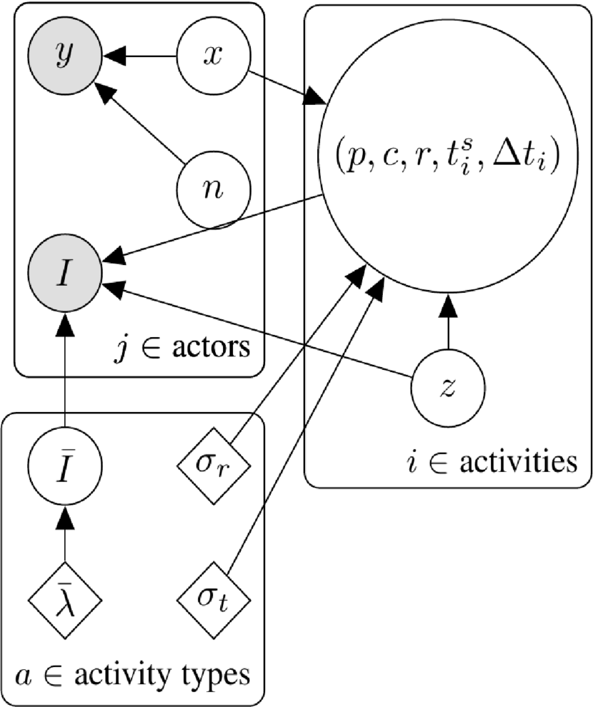
Figure 3: Proposed model for activity instance inference. Plate notation notes the separate instances of actors’ latent and observed data, activity types (here assumed to be learned in advance), and activity instances.

Figure 3 depicts the graphical model used for inference. The associated probability model for explains the observations $y,I$, as well as a latent actor trajectory $x$ in terms of the activity configuration $\{A_{i}\}$, and is given by

$$p(x,y,I|\{A_{i}\})\propto \varphi_{\textrm{GP}}(x,y|\{t_{i},\Delta t_{i},p\})\varphi_{\textrm{C}}(\{A_{i}\}|x)\times$$ (2)

$$\prod_{i}\varphi_{\textrm{SC}}(I|\bar{I},z_{i})\varphi_{\textrm{FC}}(I|\bar{I},z_{i})\varphi_{\textrm{R}}(r_{i})\varphi_{\textrm{SP}}(\Delta t_{i})\times\varphi_{\textrm{PR}}\left(A_{i}|x,p,c,r,t_{i}^{s},\Delta t_{i}\right),$$

where $\varphi_{\textrm{GP}}$ is the distribution of the Gaussian conditioned samples from Subsection 2.1. $\varphi_{C},\varphi_{SC},\varphi_{R},\varphi_{SP},\varphi_{PR}$ are factors that relate to data coverage and visual features, activity span priors and the probability for having activities. These are detailed in the remainder of the section, and specifically, Equations 1, 3, 4. While specific modeling choices are made here, modifications are conceptually straightforward. During our inference we sample for $\{A_{i}\}$ while marginalizing over $x$.

We penalize the lack of association of trajectories to an event in order to avoid the trivial result that no activities occur as follows,

$$\varphi_{\textrm{C}}\left(\{A_{i}\}|\{x\}\right)\propto\exp\left\{-c_{u}\sum_{t_{i}\in obs(p)}I_{\text{unexp}}(p,t_{i})\right\},$$ (3)

where $I_{\text{unexp}}(p,t_{i})$ is an indicator that observation $t_{i}$ of actor $p$ was not covered by any activity in $\{A_{i}\}$. This depends on the latent trajectory $x_{p}$, and the spatio-temporal span of each $A_{i}$. We set the constant $c_{u}$ empirically.

Each activity has a spatio-temporal extent with associated start time $t_{i}^{s}$ (with a uniform prior) and time span $\Delta t_{i}$. The time span is distributed as log-normal, represented by $\varphi_{\textrm{SP}}(\Delta t_{i};\mu_{t},\sigma_{t})$. Each activity is centered around a point in space where the radius of the activity is also distributed as log-normal, denoted by $\varphi_{\textrm{R}}(r_{i},\mu_{r},\sigma_{r,t})$.

Each activity has a set of associated participants where the number of participants is drawn from a discretized log-normal distribution and the identities of the participants is drawn uniformly from the set of actors. We assume that participants are present in the spatial extent for the duration of the activity, centered around point $c_{i}$ (uniformly sampled). This is captured by a factor

$$\varphi_{\textrm{PR}}\left(A_{i}|\begin{matrix}\{x\},p,c,r,\\ t_{i}^{s},\Delta t_{i}\end{matrix}\right)\propto\exp\left\{-\int h_{r_{i}}^{c_{i}}(x,t)dt\right\},$$ (4)

where $h_{r_{i}}^{c_{i}}$ is an indicator function limiting excursion of trajectory $x$ to a maximum distance $r_{i}$ from the center $c_{i}$ at time $t$.

We incorporate scene classification features as visual cues for each frame using the Places CNN model [37]. We associate frames with each activity according to whether or not their location and time is within the span of the activity. The probability of each scene classifier is modeled as a normal, separable distribution in both features and frames, $\varphi_{\textrm{SC}}(I|\bar{I},z)\propto\prod_{v}N(\mu_{v,z},\sigma_{v,z}^{2})$. $\mu_{v,z}$ and $\sigma_{v,z}^{2}$ represent the mean and variance of each meeting type’s visual content, per the Places feature, and $z$ represents the activity type. These were estimated based on a set of photos taken at the same locations as the experiments.

Face detections are also used as a visual cues. We use face frontalization [13] and one-shot similarity kernels [31], along with a set of precollected and annotated face examples to detect and recognize people in the video, thus creating a set of detection streams. Given an activity and its participants, we treat the detections of each actor as counts from a Poisson process with either a high rate $\lambda^{p}_{p}$ if the actor $p$ is a participant, or a low rate $\lambda^{n}_{p}$ if the actor is not a participant in the activity.

2.3 Conditioning Trajectories on Activities

For a given activity instance, the participants are more likely to be at the same location, depending on activity type. While this is captured by the spatial factor in Equation 4, we may have impoverished samples e.g., due to GPS denial. In such cases, the trajectories of all participants traveling outside the spatial extent of the activity should be rare event and should be sampled judiciously. While rare events in Gaussian random fields have been studied extensively, the majority of the work has been on excursion sets which are less applicable in our case (see [1, 19] and references therein).

We accommodate this concern in the following manner. Given a sampled configuration, we condition on auxiliary observations of the proximity of the participants. For spatially static activities such as the ones we show in Section 4, the auxiliary observations have the form

$$0=x_{p}(t)-\frac{1}{|P_{a}|T}\sum x_{p^{\prime}}(t)+n_{(p,a)}(t).$$

A different set of auxiliary observations, suitable for dynamic group activities is shown in Appendix A. Once we have added the auxiliary observations, we condition on all observations to obtain samples of the latent trajectories (which are now statistically dependent). This can be seen in Figure 7(g,h), when determining the conditioned trajectories, but we note that for the scenarios we show in Section 4, the GPS denial periods were sufficiently short to inference the activities regardless of this problem.

3 Activity Summarization and Analysis

We now describe the inference procedures relevant for our activity model, and our use of it for summarization and localization.

3.1 Activity Inference

As noted previously, reasoning over activities utilizes inferred trajectories, in our case samples from $p(x|y)$ via standard Gaussian process inference. We derive an MCMC procedure for the remaining variables. There are several methods for inference in stationary Gaussian processes affording efficient implementation and online processing [14, 12, 6]. For our purposes, we found equidistant sampling in time and matrix inversion sufficient to provide trajectory estimates. We used a variant of reversible-jump MCMC (RJ-MCMC, [10]), in order to infer activities. The steps we used include Birth/Death, Split/Merge, and parameter modification for $\Delta t,t_{i}^{s},c_{i},r_{i}$ and the participants. The full set of allowed steps is described in Appendix B. The number of burn-in iterations required depends on the number of activities, participants, time samples, and the relative identifiability of the activities. In the examples shown in Section 4, $\sim 10^{4}$ iterations sufficed.

Algorithm 1 Estimating activities by RJ-MCMC

1:  for $i=1,2,\dots,N_{hist}$ do

2:     Choose a step type: birth/death, split/merge, or type, center, radius, span, start-time and participants changes, see Appendix B. for the description of each step.

3:     Update GP observations according to Subsection 2.3 (optional).

4:     Compute proposed new configuration and its acceptance probability based on the model at 2.

5:     Update configuration if accepted, if $i>N_{burn-in}$, save configuration samples

6:  end for

3.2 Collaborative Localization

Our model enables improved localization by associating data streams via activities, even in the face of sparse GPS measurements. For a set of trajectories $x$ we have:

$$p(x|A,y,\theta)=p(A,x|y,\theta)/p(A|y,\theta)\propto p(A|x)p(x|y,\theta)$$ (5)

via Bayes rule and the dependency structure. Marginalizing over the sampled set of configurations, we can reduce uncertainty based on interactions with other actors, as demonstrated in Section 4.3.

3.3 Collaborative Summarization

An important aspect of collaborative summarization that we demonstrate is keyframe selection that emphasizes activities of interest. We do so using a farthest-point-sampling approach (FPS, [9, 15]), with an appropriate metric between frame pairs (see Appendix C for full details). We say that two frames disagree with respect to an activity if one of them was sampled as a part of this activity, and the other was not.

We denote by $d_{AC}(f_{i},f_{j})$ a measure of disagreement between frames $f_{i},f_{j}$ marginalized over activity configurations. The distance between two frames is a positive linear combination of $d_{AC}$ as well as the feature-space, temporal, and participant identities distances. It is a metric, as required for FPS. Sampled keyframes are reordered according to time. When selecting keyframes, we pick only from those that are likely to have participated in the relevant activities or in the relevant actors’ datastream. The selected frames can be used for a video summary, or a map-based summary using their inferred locations.

Algorithm 2 Keyframe selection for collaborative activities

1:  Initialize counts to be $0$

2:  for All configurations $\{A_{i}\}$ and activities $i$ do

3:     for All actors $a$ and frames $t$  do

4:        If actor’s frame is within activity $i$’s span, add a vote.

5:     end for

6:  end for

7:  Remove keyframes with low votes count, compute frame-pair distances.

8:  Sample keyframes via FPS, re-order keyframes according to time.

Video Summarization For the case of videos, tradeoff between information variability and film consistency is used, similar to Arev et al. [2] (but using only epipolar geometry and average image motion in the absence of 3D metric reconstruction).

Map-based Summarization For a summary image, we overlay relevant frames on a map of the area, by placing keyframes inside the area defined by each activity’s center and radius. We use FPS in order to place the frames uniformly.

4 Results

We first explore the use of our algorithm on a synthetic dataset to ensure accurate detection of activities under model circumstances, then proceed to demonstrate activity inference, summarization, and localization in the case of real-world wearable data.

4.1 Activity Inference

We now demonstrate the result of inferring plausible configurations of activities on a synthetic dataset generated according to the following structure: at each turn, each of eight actors can either go to one of several meeting places, or go to their own random location. If two or more actors are at the same location, this constitutes an activity. We test the inference procedure on this model. When meeting places are well-separated from each other (compared to the observation noise and typical meeting radius), we can infer activities without difficulties. Figure 4 explores the increase in detection errors as a function of the standard deviation of the meeting locations, over multiple realizations. The distribution of meeting locations should be contrasted with a measurement noise of 30 meters, and meeting radius distributed with $\mu_{r}=30$, and a meeting-times prior set to log-normal with parameters $\mu_{t}=60,\sigma_{t}=0.05$. Looking at detected activities, the main source for false detection occurs when actors unintentionally cross paths for prolonged periods of time.

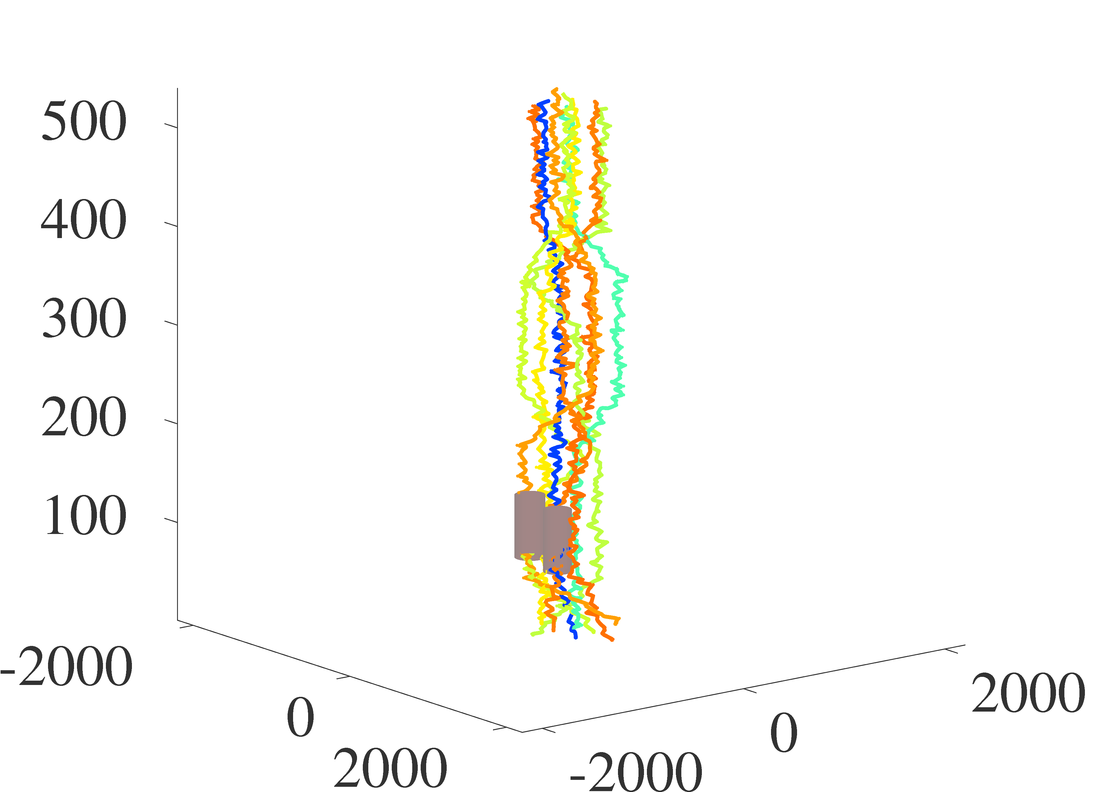
(a)

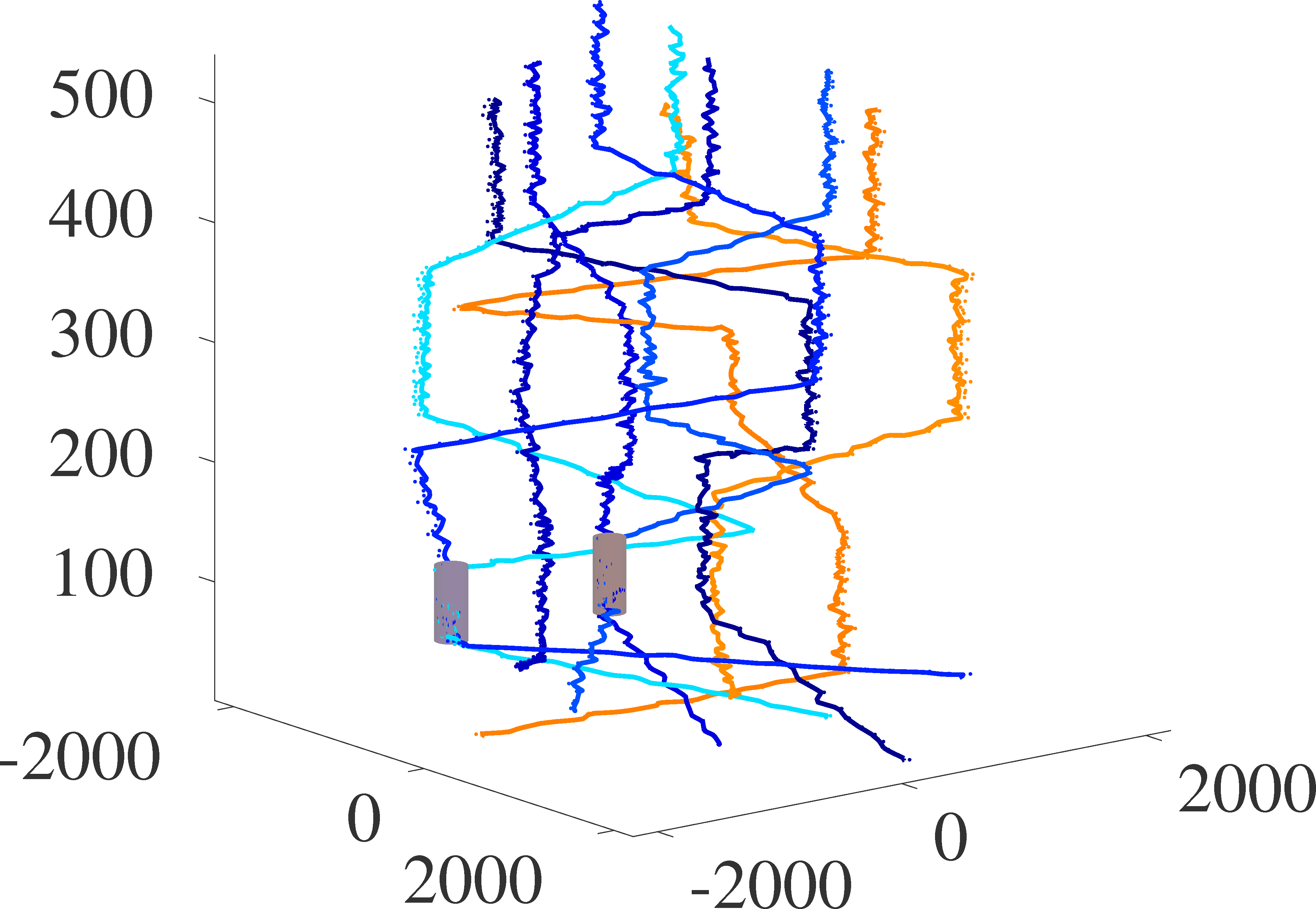
(b)

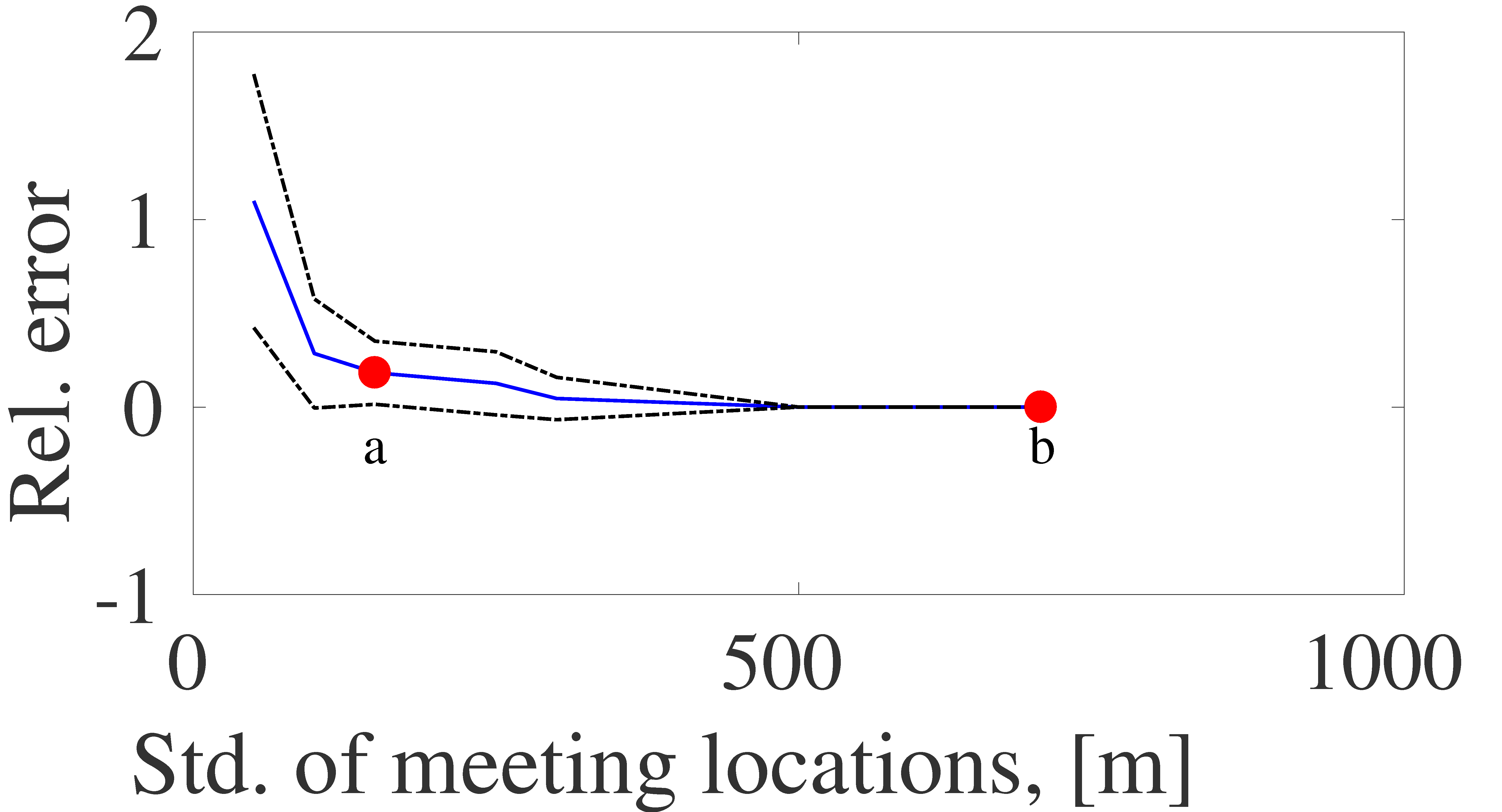
(c)

Figure 4: Example results from synthetic experiment of meetings among eight actors. (a),(b) Left subfigures: example trajectories and detected configurations, for different distributions of meetings’ locations. The $x,y$ axes represent spatial dimensions and the vertical axis represents time shown from two viewpoints. The std. of activity locations in (a),(b) is 150 and 700 meters, respectively, compared to GPS noise and activity mean radius of 30 meters. Different colored ensembles of curves represent five estimated tracks from each participant, based on GPS observations (marked as dots). Cylinders mark the spatio-temporal span of detected activities. Right: the relative error in the estimation of the number of activities, averaged over 20 trials, black dashed lines mark $\pm 1$ std. curves. The 2 red dots show the std. for Subfigures a,b. As can be seen, algorithm manages to detect the activities even when they are barely discernible in the GPS observations.

We now demonstrate activity inference on a real dataset, available at [24]. This dataset includes four actors walking for half an hour in an urban area spanning 600 meters, and meeting each other, either on the street (activity type 1) or inside a coffeeshop (activity type 2). During a training phase, we construct our feature priors based on a subset of images from such locations so as to identify the two activity types with this semantic categorization. The actors are wearing GoPro cameras that provide a partial, egocentric video, with over $2300$ classified face tracklets in the videos. The error rate for face detection in the video was $14\%$, giving us a noisy, but informative, signal.

During some of the meetings, GPS reception was poor with gaps ranging from one to nine minutes in duration, in the GPS coordinate measurements of some participants. Furthermore, ten minutes of video were removed from participant number four, in order to test data pooling from different sources. As can be shown in Figure 5, all meetings are detected in a stable manner, despite missing GPS. This dataset is simple enough to be easily understood, and yet captures a lot of the difficulties in understanding and summarizing collaborative interactions in a realistic urban environment. An additional example, also included in [24], with $11$ participants is shown in Subsection 4.5. While the urban environment and multiple activities makes interpretation of results more difficult in this example, we are still able to detect most of the activities and demonstrate how the approach scales up for more complex data.

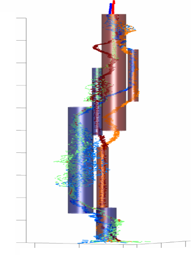
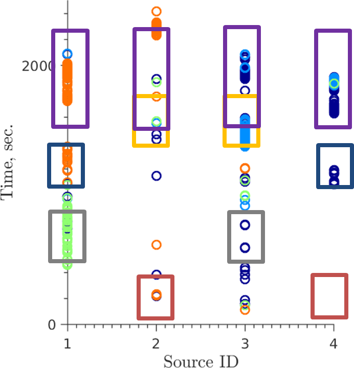
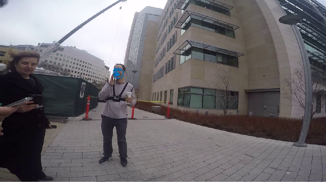
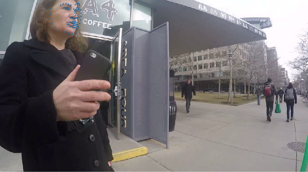
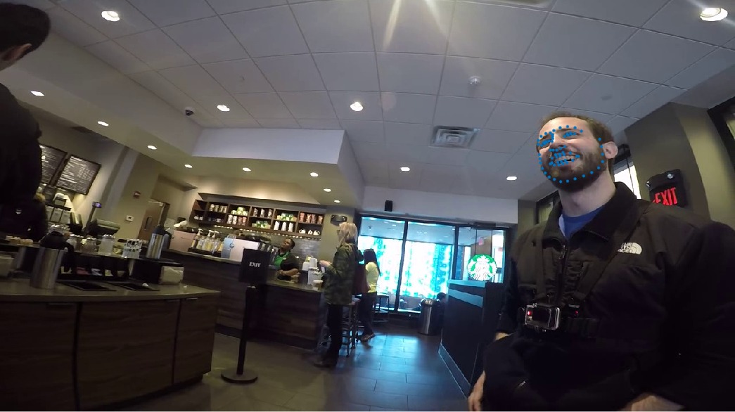
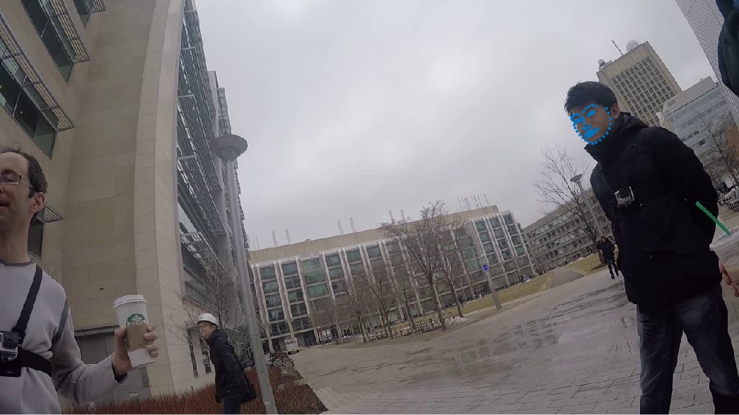
(a)

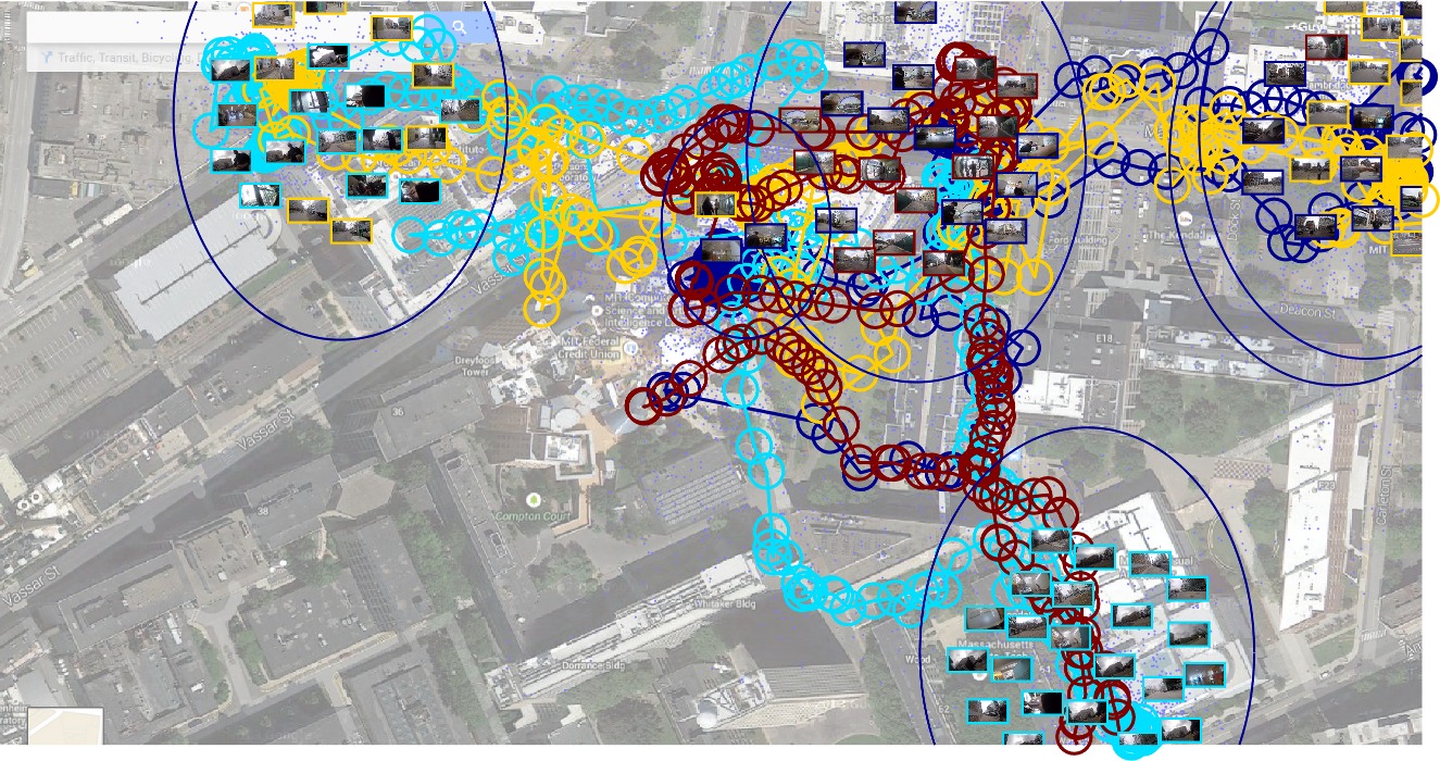
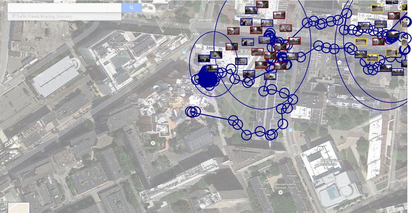
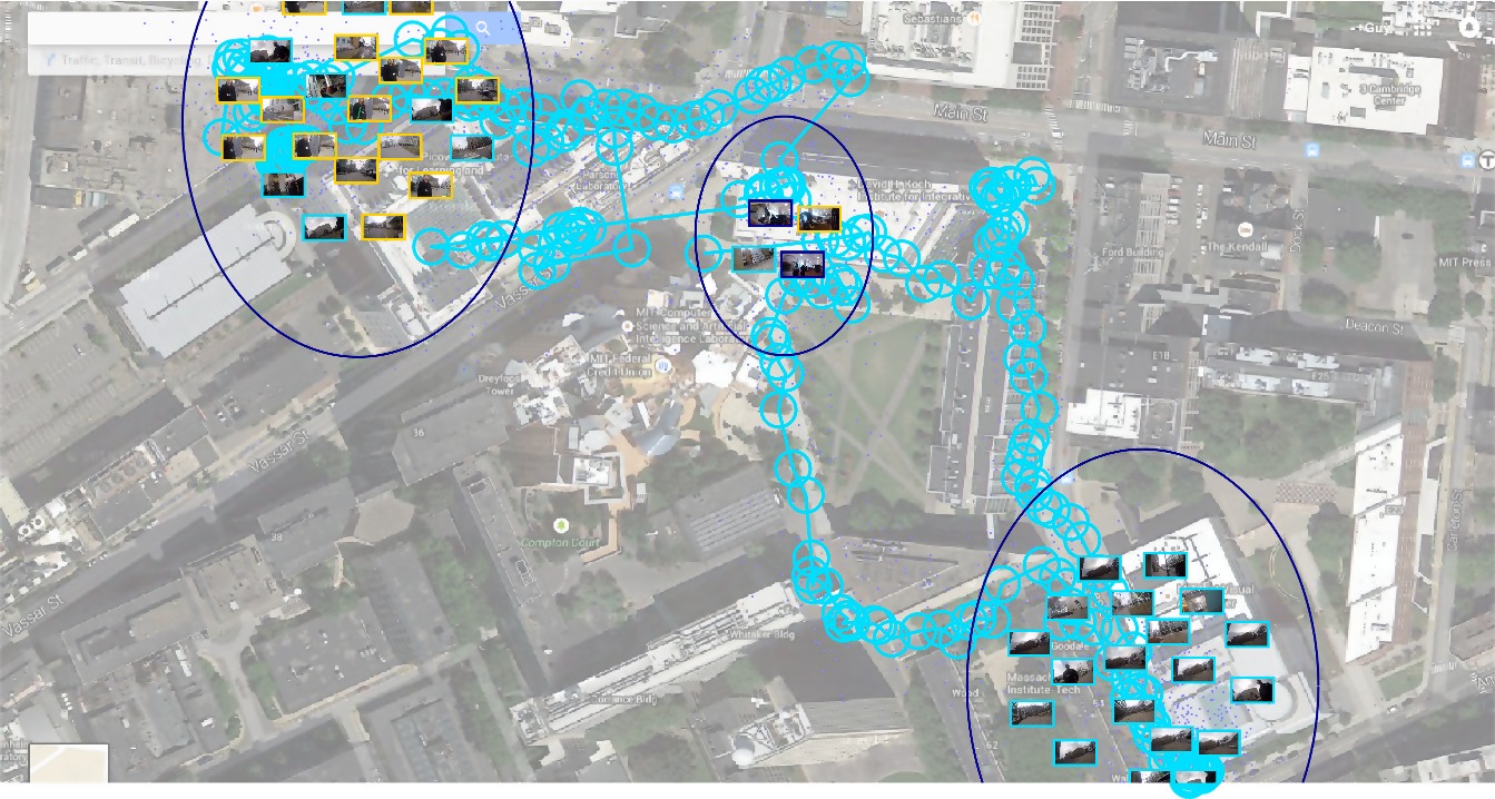
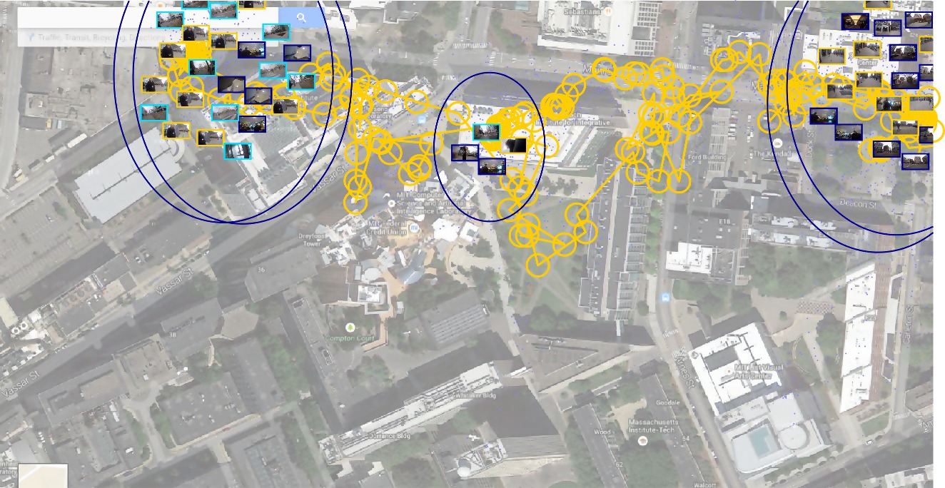
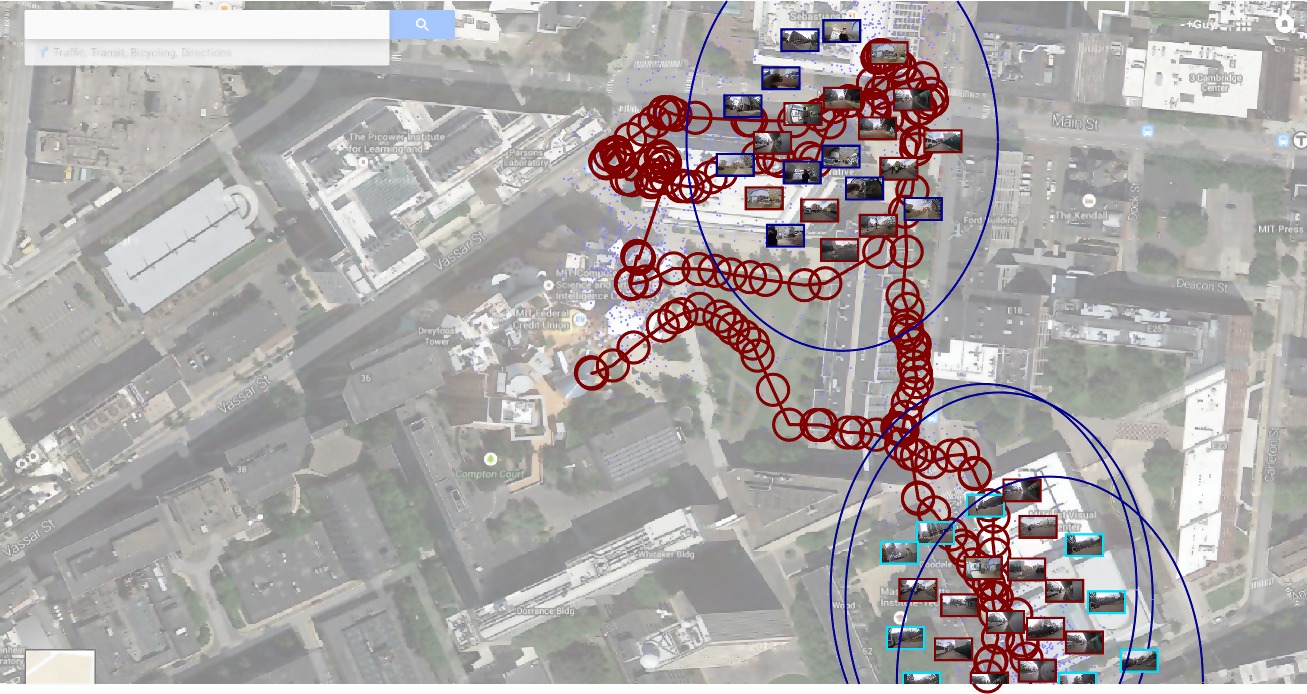
(b)

Figure 5: a) Left: Activities detected on our dataset, with four actors walking and interacting for approx. 30 minutes. Blue cylinders represent indoor meetings, whereas red cylinders represent outdoor meetings. Right: a time plot of detected faces in the different actors’ video feed, overlayed with a ground-truth of the meetings that took place. As can be seen, all meetings were detected, and are to some extent evident in the face detection streams. b) Top: summarization of actors activities with respect to the map, based on the GPS and video footage of $4$ actors. Colored trajectories represent actors GPS location measurements, using the same actor color as Figure 6. Circles mark the trace of detected activities, with representative frames displayed on top. Bottom: the individual four actors storylines, with activities depicted based on the pooled actors’ video footage. The map and images have been blurred for review.

4.2 Summarization

In Figure 6 we demonstrate the summarization of actors’ data from all four actors. Rows (a)-(d) summarize individual actors’ timeline, pooling footage from other actors who participated in that actor’s activities. The fifth row summarizes the data from all four actors and activities, whereas the sixth row summarizes all actors but favoring frames from “coffeeshop” activities. Summarization is done while attempting to balance content and time variability, and activity representation, as described in Subsection 3.3. We highlight the beginning of actor 4’s storyline. This actor’s video data for the first few minutes was removed from the set, and yet, the algorithm has completed it due to the detection of a meeting between actors 3,4.

In Figure 5 we demonstrate the summarization of activities on a map. The GPS measurement locations are shown for each actor on the map, and demonstrate the noisy raw data used to estimate the locations and infer the activities. Green circles represent a set of detected activities. Inside each circle, several images are placed and represent main parts of the meeting.

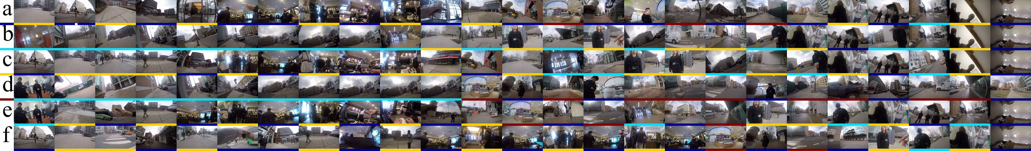
Figure 6: Rows (a)-(d): summarization for actors 1-4, utilizing footage from likely participants in each actor’s activities, going left to right. See left size colors legend and frame color to mark the frame source. Row (e): A combined storyline of the four actors, using images from all of them. Row (f) All four actors, but with emphasis on activities that are likely a “coffeeshop”. Note how in the beginning of the timeline, (d) takes footage from participant (b) during their activity, whereas actors (a),(c) share footage. The ending is similar for most participants due to a final joint meeting.

4.3 Localization

Our model allows us to better localize actors from partial GPS measurements, through the GP samples, and the posterior likelihood of the trajectories. We use Equation 5 to visualize a sampled trajectory set for each actor. While ignoring trajectories dependence, this visualizes likely trajectories for each actor, as shown in Figure 7 for two actors in a GPS-denied cafe for about ten minutes, starting at $t=500$. While their location is less certain, conditioning on the sampled configurations allows us to better localize them better. The average standard deviation of the two participants $(1,3)$ during that meeting dropped from $(73,90)[m]$ to $(53,57)[m]$, respectively. The same phenomenon can be seen for shorter GPS denial segments as well, around $t=1250$, with reduction in standard deviation for participants $(1,4)$ from $(66,68)[m]$ to $(53,44)[m]$, respectively. This shows halving of the variance in such cases.

While for this example linear interpolation may work in a low-noise setting, our GP model allows activities where participants are moving together (e.g., field-trip or running group).

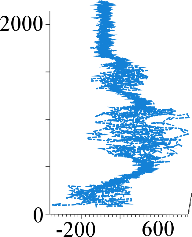
(a)

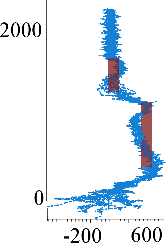
(b)

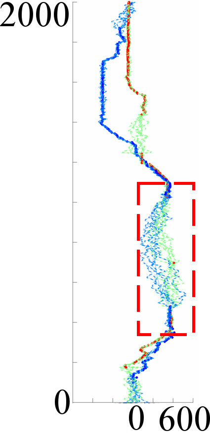
(c)

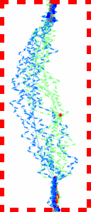
(d)

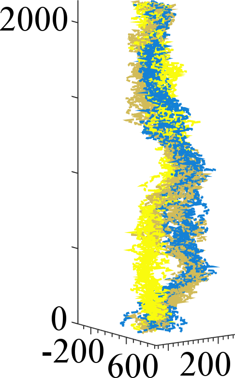
(e)

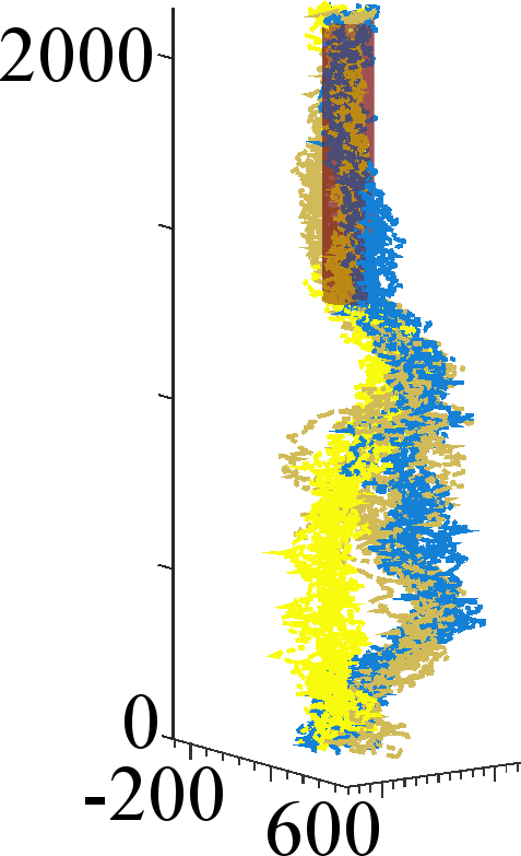
(f)

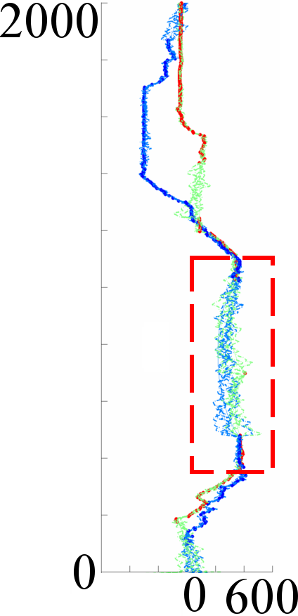
(g)

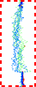
(h)

Figure 7: (a),(b): Estimated GP trajectories for a single actor, as $(x_{1},x_{2},t)$, with units $([\mbox{m}],[\mbox{s}])$, before and after conditioning on sampled activities (shown as a maroon cylinders). Note the divergence of samples once GP measurements are missing, where actors are inside a building. (e),(f): The trajectories of two participants before and after conditioning on an activity. (c),(d) and (g),(h) Max-likelihood trajectories of two participants holding a meeting (around 500 seconds, on the $z$ axis) – full and zoomed view of $x$ conditioned on observations $y$, followed by $x$ conditioned on the detected activities configuration $\{A_{i}\}$ and $y$. Clearly by conditioning on $\{A_{i}\}$ we can better localize the two people despite GPS-denial.

4.4 Prior for Face Recognition

We compute a conditional probability of facial features given participant identity and the maximum-likelihood configuration, as described in Subsection 2.2. This lowers the face recognition error on average by $5.5\%$, demonstrating the utility of a unified multimodal model for explaining the data.

In Figure 8 we demonstrate several examples where incorrect face recognitions were corrected, conditioned on the inferred activities. While there is no guarantee the conditional probability always improves recognitions, in our specific case we did not see such examples. While the face recognition network used is relatively simple, the factors leading to incorrect labelling in those cases are relevant for even state-of-the-art classifiers [27], and include partial occlusions and reflections as a face is seen through a glass door.

Assuming independent activities $A_{i}$, we write the probability of a specific detection’s identity to be

$$p(a|\{A_{i}\})\propto\prod_{i}p(a|A_{i}),$$ (6)

where $p(a|A_{i})$ is uniform for all activity participants, with a small non-zero value for non-participants. Plugging Equation 6 into Equation 11 in the main paper results in an additive term for the log-likelihood. Normalizing w.r.t the partition function gives us the modified face detection probabilities.

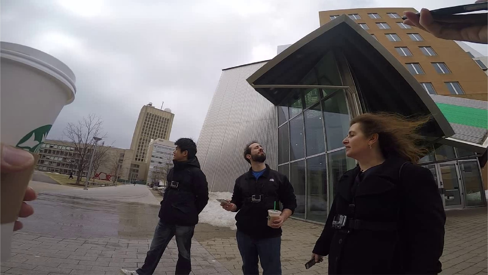
(a) Classifier: unrecognized. Posterior: Participant 2.

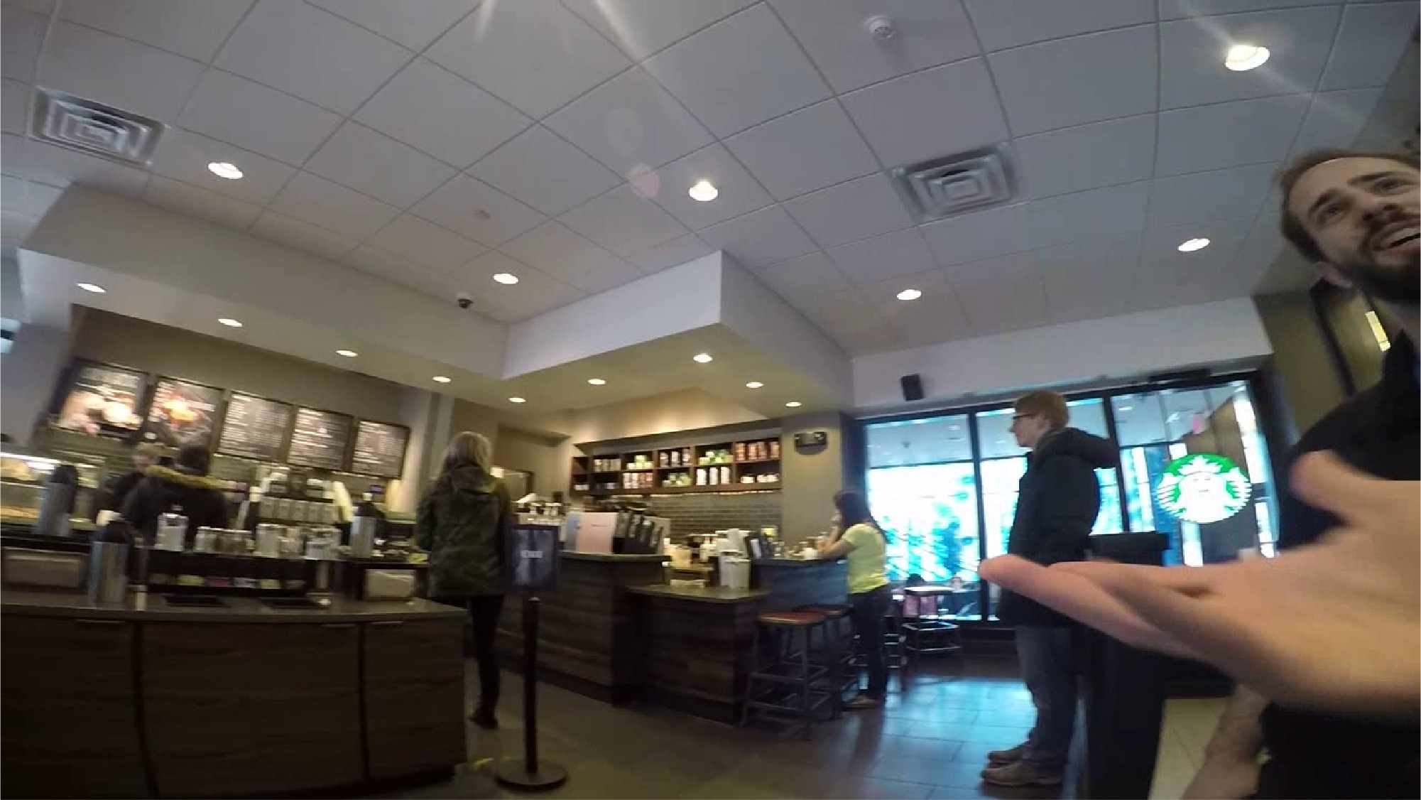
(b) Classifier: participant 1. Posterior: participant 3.

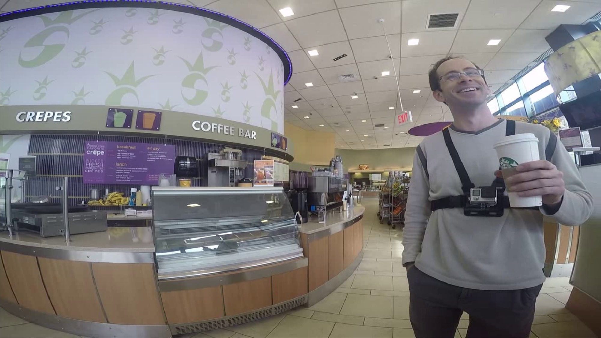
(c) Classifier: participant 3. Posterior: participant 1.

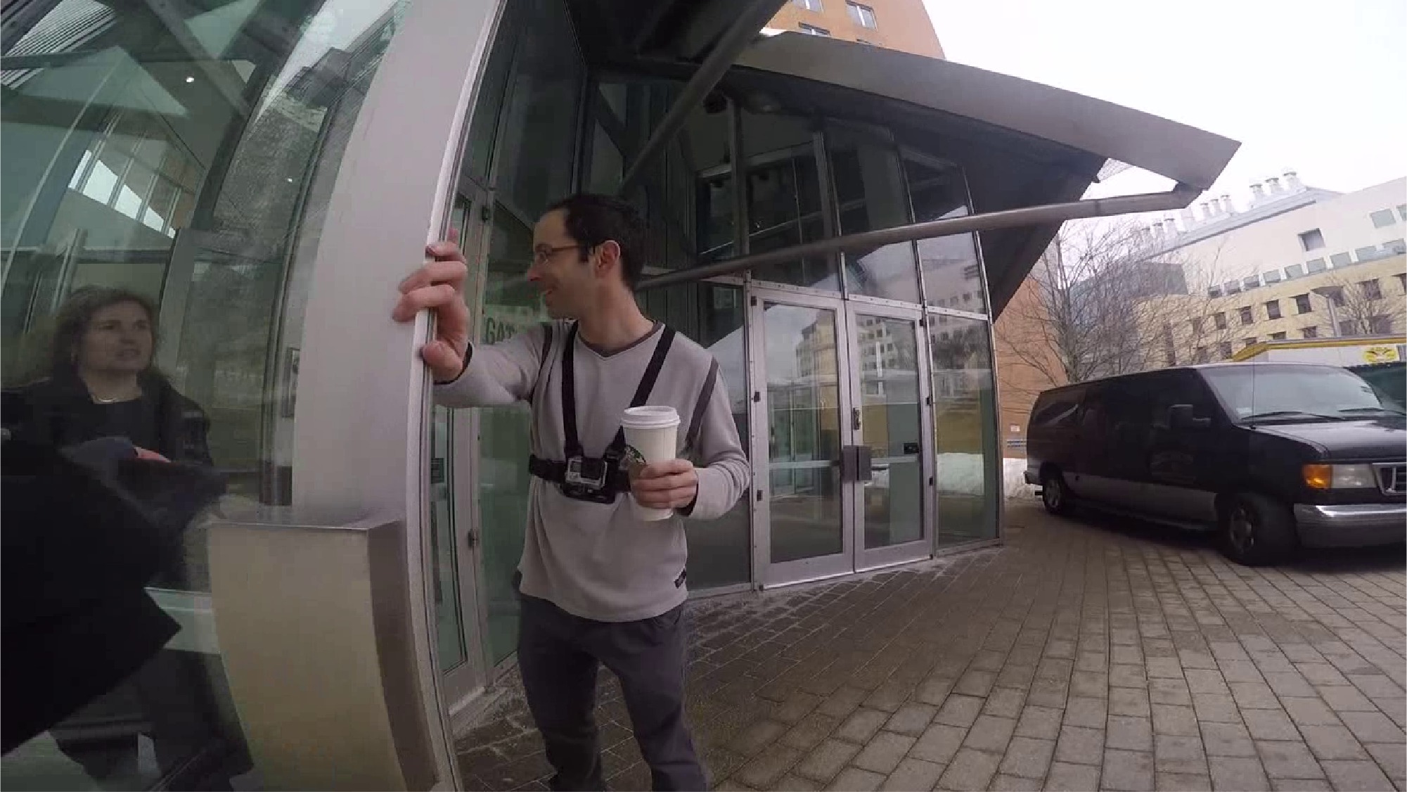
(d) Classifier: unrecognized. Posterior: Participant 2.

Figure 8: Example face correction, based on the detected activities. Some examples were inherently difficult to recognize despite rectification and alignment, due to partiality (a,b) and reflections (d).

4.5 Larger-scale Scenario

We now demonstrate the activities detected on a larger scale scenario. In this experiment, 11 participants were asked to walk in an urban area 800 meters across, and meet other participants for 3 or more minutes at each time, for 90 minutes (overall 1000 minutes, and more than 20 interactions). The resulting detected activities, and the participants raw GPS trajectories that participated in each configuration are shown in Figure 9. While not all configurations sampled contain all activities, we cover the set of expected activities and locations, as can be seen in the Figures 9,10. While the complexity of the scenario makes the visualization crowded, one can observe the scale of examples for which we can infer configurations, despite the limitation of MCMC methods in high-dimensions. We note that the locations and times match the locations reported by participants upto the localization artifacts expected in an urban area, with similar detection results as in the 4-participants example shown in the paper.

Figure 9: Top two rows: example configurations sampled during the RJ-MCMC step (black circles), along with their corresponding participants’ GPS measurements (multicolor line and circle). Bottom two rows: the activities related to four out of the 11 participants (black circles), and their estimated GP trajectories (light blue line and circle).

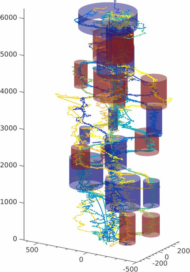
Figure 10: Spatio-temporal plot of the maximum-probability configuration of activities. the vertical axis denotes time, the horizontal axes denote space. Cylinders denote detected activities. The paths denote samples of the GP trajectories of all 11 participants. As can be seen, most meetings were detected in this configurations.

5 Conclusions

In this report we showed how a simple set of assumptions on social interactions leads to a model that enables collaborative activity summarization and improved localization under noisy and missing sensory streams. We demonstrate how a sampling-based strategy affords meaningful analysis even when the data is partial and noisy to the point that activities cannot be identified with certainty. We expect additional observation models to allow extension of this framework to more refined activity classification and summarization, also for individual activities, as well as semantically-assisted GPS localization.

Appendix A: Collaborative Dynamical Models

We now elaborate on the auxiliary observations mentioned in Subsection 2.3 of the paper. Given a set of activities $\{A_{i}\}$, we model them as observations tying participant locations to the activity. We propose two typical models, though other models can also be proposed.

Dynamic model - in this model, we expect each participant to be at the same location as all other participants at every time instance. The location is not fixed and the group can move about. This is modeled by observations of the form

$$x_{p}(t)-x_{p}^{\prime}(t)=n_{p,p^{\prime},t},n_{p,p^{\prime},t}\sim\mathcal{N}(0,\sigma^{2})$$ (7)

for each participants pair $(p,p^{\prime})$, time instance $t$, within the span of activity $A_{i}$.

Static model - in this model, we expect each participant to be at the same average location as are the other participants throughout the activity. We do not force the specific location, but do expect it to be fixed for the duration of the activity.

$$x_{p}(t)-\sum_{p^{\prime}\in A}\int_{t^{\prime}\in span{A}}x_{p^{\prime}}(t)dt=n_{p,t},n_{p,t}\sim\mathcal{N}(0,\sigma^{2})$$ (8)

for each participant $p$ and time $t$ in the span of activity $A_{i}$.

We note that both of these terms are linear observations with additive white Gaussian noise, and hence conditioning can be done by Gaussian belief propagation [29]. Finally, in order to compute the acceptance ratio, we compute the determinant of the conditioned covariance matrix. This can be done with Cholesky factorization although faster approximations have been proposed (see, for example, [11]).

Appendix B: MCMC Steps

We now describe the MCMC steps used to infer the configuration of activities. Model inference uses a set of Gaussian process samples: 500 samples for each actor, sparsely updated. Our inference procedure includes the following steps, illustrated in Table 1.

Dimensionality Changing Steps

Birth - In order to create a new activity, we first draw the number of participants based on a discretized log-Normal distribution

$$\hat{|p|}\sim\lfloor\log\mathcal{N}(2,0.5)\rceil,\ \ \ |p|=max(\hat{|p|},2)$$ (9)

given the number of participants, we sample $|p|$ participants uniformly from all actors. We sample the start time uniformly from the relevant measurements’ support, and then the span. The prior distribution for the span is given as

$$\Delta t\sim\log\mathcal{N}(300,0.01),$$ (10)

Death - We propose death events (i.e removal of an activity from the configuration) by sampling uniformly from the existing activity, and compute the probability of the remaining activities after removal of one, for the acceptance probability.

Split - We split events along the time axis by uniformly sampling a split point along the old span of the activity.

Merge - We merge two activities by taking the participants set and spatial support of one of the activities, and merging the convexification of the two events’ temporal spans. While a similar approach, of choosing a minimal circle to include the two existing activities could be done for the spatial support, we found it to be unnecessary in practice.

	Before	After
Birth
Death
Split
Merge
Type
Center
Radius
Span
Participants

Table 1: Illustration of the MCMC steps used in the proposed activity detection algorithm. Blue curves represent participants trajectories, red and blue boxes portray two different types of activities.

Parameter Changing Steps

These are MCMC steps that do not modify the number of activities but rather their attributes. They are: type, center, radius, span, start-time and participants of activities.

Type - We sample uniformly from all activity types, and compute the proposed activities’ probabilities conditioned on the sampled trajectories.

Center - We recompute the center of each activity by sampling with an additive Gaussian displacement around the set of estimated GPS Gaussian process samples. This limits our proposal distribution to be around the areas that are relevant, assuming relatively mild GPS denial.

Radius - We use a proposal distribution for the radius,

$$q_{r}\sim\log\mathcal{N}(30,0.03).$$ (11)

Span - We sample the span according to a proposal distribution that differs from its prior distribution in order to accomodate wider variations, as supported by the data. the proposal distribution is

$$q_{s}\sim\log\mathcal{N}(300,0.005).$$ (12)

Start-time - we sample the start-time $t_{i}$ uniformly from the temporal span of the measurements.

Participants - we resample participants according to the prior distribution of $|p|$ and the uniform assumption for participants’ identities.

Appendix C: Video Summarization

We detail how to create a the video summarization as shown in the supplementary video, based on the frames selected in Section 3.3 of the paper. Considerations guiding the design of our video summarization include:

• Variety & Model Relevance:

  • Output frames should be balanced between desired actors, times and locations

  • Output frames should emphasize inferred activities.

• Aesthetics:

  • Output frames should not be noisy, motion-blurred or of low content.

  • Frames should not frequently/abruptly switch viewpoints/actors.

Graph Formulation, Edge and Node Weights

Summarization is formulated as an approximate, constrained shortest-path problem on a trellis graph, similar to [2], but utilizing the sampled GPs, activities, and faces models from RJ-MCMC inference. The trellis contains $m$ rows, one for each video stream, and has columns equal to the maximum number of image frames associated with any actor. Each node, $V_{i}^{t}$, corresponding to actor $i$’s possible output image at time $t$, is associated with $f_{i}^{t}$, the candidate image frames of actor $i$ at output frame $t$. We assume that if $|f_{i}^{t}|=0$, then it will never be chosen for time $t$ (since it has no image to contribute). All nodes $V_{i}^{t}$ are connected to all nodes $V_{i}^{t+1}$ by edges $E_{i,j}^{t}$, and both nodes and edges are weighted.

Nodes are weighted according to quality and level-of-activity metrics, edges according to inter-frame distances with respect to sampled time and location, activity and observed-participant continuity, as well as shared viewpoint. Node weights are computed as cost $C(V_{i}^{t})=C(f_{i}^{t})$, where $f_{i}^{t}$ is actor $i$’s candidate frame for time $t$:

$$C(f_{i}^{t})=\left(\left(1-\frac{|{kp}_{i}^{t}|}{\overline{kp}}\right)w_{q}+\delta_{f}w_{f}+\delta_{a}w_{a}\right)w_{i}$$ (13)

Where ${kp}_{i}^{t}$ are the SURF keypoints detected in frame $f_{i}^{t}$, $\overline{kp}=\max_{i,t}|{kp}_{i}^{t}|$ is a normalizer, $\delta_{a}$ is an indicator variable of whether a participant has been identified in frame $f_{i}^{t}$, and $\delta_{a}$ is an indicator of whether $f_{i}^{t}$ belongs to an activity (i.e. $f_{i}^{t}$ is associated to actor $i$ who participates in an activity, and $t$ is within that activity’s span). Weights $w_{q},w_{f},w_{a}$ control relative importance and $w_{i}$ is a discount factor on the total cost for actor $i$ (useful for favoring / excluding certain actors).

Although edge weights are computed between nodes $V_{i}^{t}$ and $V_{j}^{t+1}$, they are in actuality functions of candidate frames $f_{i}^{t}$ and $f_{j}^{t+1}$, computed as the distance:

$$d(f_{i}^{t},f_{j}^{t+1}) =\left(\left((1-\frac{M({kp}_{i}^{t},{kp}_{j}^{t+1})}{\overline{M}({kp})}w_{\text{nm}}\right)+(1-\delta_{\text{sf}})w_{\text{sf}}+(1-\delta_{\text{sa}})w_{\text{sa}}\right.$$

$$+\qquad\left.\vphantom{\int_{t}}\Delta_{i,t}^{j,t+1}w_{\Delta}+\mathcal{T}_{i,t}^{j,t+1}w_{\mathcal{T}}\right)\delta_{\mathcal{N}}w_{\mathcal{N}}$$ (14)

Where $M({kp}_{i}^{t},{kp}_{j}^{t+1})$ are the number of matched keypoints between keypoints ${kp}_{i}^{t}$, ${kp}_{j}^{t+1}$ (defined above) and $\overline{M}({kp})=\max_{i,t,j,t+1}M({kp}_{i}^{t},{kp}_{j}^{t+1})$ is a normalizer. $\delta_{\text{sf}}$ is an indicator for whether the same participant is detected between frames $f_{i}^{t},f_{j}^{t+1}$, and $\delta_{\text{sa}}$ is an indicator for whether the two frames belong to the same activity. $\Delta_{i,t}^{j,t+1}$ is the L2 spatial distance (marginalized from GP coordinates) between the location of actors $i$ and $j$ at the times when frames $k$ and $l$ were taken, and $\mathcal{T}_{i,t}^{j,t+1}$ is the L2 temporal distance between the times that frames $f_{i}^{t}$, $f_{j}^{t+1}$ were taken for actors $i,j$ at times $t,t+1$, respectively. $\delta_{\mathcal{N}}$ is an indicator of whether frame $f_{j}^{t+1}$ belongs to a new activity relative to previous frame selections, and $w_{\mathcal{N}}$ is the discount factor applied in such a case.

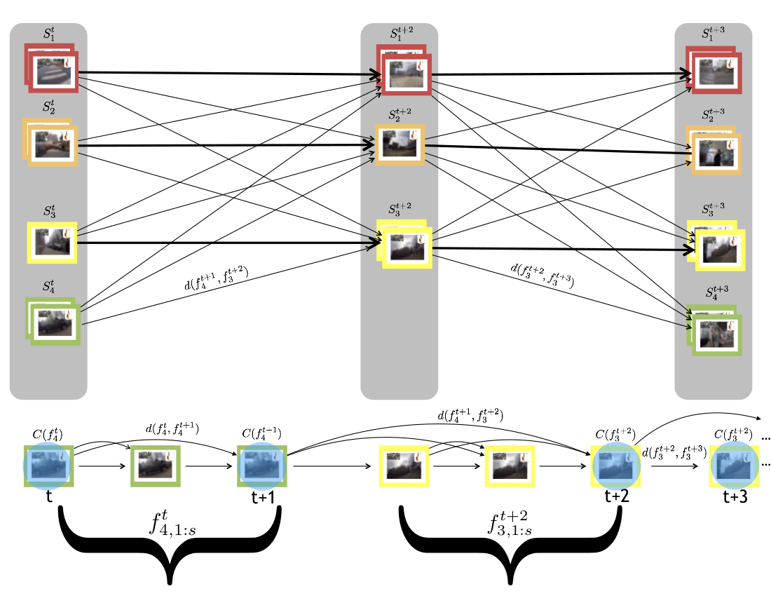
Figure 11: Illustration of the Super Trellis constrution used for video summarization. Rows correspond to actors (here, there are four), whereas a column at time $t$ is responsible for anywhere from $1,\ldots,s$ output frames, where in this case $s=3$. Example Super Nodes are shown below the trellis, where $S_{4}^{t}$ contains frames $f_{4,1:s}^{t}$, and for which the first and third (translucent blue circles) were chosen as the lowest-cost output frames among all candidate Super Nodes $S_{i}^{t}$ for the first column. In this case, there is a toy constraint that the minimum and maximum number of consecutive output frames from a single actor are both $2$. Hence $S_{4}^{t+2}$ is not reachable in the second column (despite likely having frames associated with it) and so is omitted from the graph. Note also how at time $t+2$, only one frame was chosen from Super Node $S_{3}^{t+2}$, hence, by the constraint, $S_{3}^{t+3}$ must be chosen in the next column, though from that, only one node will be selected. There will typically be more observations, $f_{i,1:s}^{t}$ in Super Node $S_{i}^{t}$ than selected output frames. Note that here, only the edge and node costs that contributed to the actually-chosen path are displayed.

Constraint Handling

Although the above costs empirically make good decisions about actor and activity coverage, the resulting summarization includes rapid transitions between actors’ video feeds that are visually unpleasant for observers. To solve this, and to increase control over the types of summaries produced, our summarization supports the following constraints $c_{1}$: beginning/end time $t_{\text{begin}}$, $t_{\text{end}}$, $c_{2}$: permitted/prohibited locations, $c_{3}$: max temporal jump between successive output frames, and $c_{4}$: min/max consecutive frames with respect to an actor. Though incorporation of these constraints force an approximate, greedy solution rather than a true shortest-path via Viterbi decoding, significantly more aesthetic videos are produced as a result, and computation is faster.

Super Trellis and Super Node Construction

To provide our algorithm the ability to "look ahead" (i.e. not make frame-wise greedy decisions) and to ease the enforcement of constraint $c_{4}$, we pool nodes along each row of the trellis into "Super Nodes" with pre-specified maximum size of $s$ nodes. These Super Nodes can be said to form a "Super Trellis" where, again, rows correspond to actors, but now each node corresponds to frames $f_{i,1:s}$ for actor $i$. At each step through this Super Trellis the min-cost path is computed within each Super Node, and then the min-cost Super Node is chosen. Hence, columns in the Super Trellis correspond to as many as $s$ time steps in the original, frame-wise trellis. Node and edge costs in the Super Trellis are handled as one would expect: edge weights between Super Nodes are computed as the edge weights between the last frame of the previous Super Node and the first frame of the next, and edges weights within Super Nodes are computed as originally specified, though they are always between frames of the same actor. The cost of each Super Node, then, is the sum of the internal node and edge costs of the greedy-selected min-cost path within it (which, though it always moves forward in time, need not select all frames). Details of this algorithm are specified in Algorithm (3).

Algorithm 3 Collaborative Activity-Based Video Summarization

1:  Given actors $a_{i=1:m}$, activity set $A_{1:n}$, actors’ image sets $f_{i,:}$ with corresponding face recognitions $r_{i,:}$, desired number of output frames, $T$, as well as parameters $w_{q},w_{f},w_{a},w_{i},w_{\text{am}},w_{\text{sf}},w_{\text{sa}},w_{\Delta},w_{\mathcal{T}},w_{\mathcal{N}}$, super-node size $s$ and constraints $c_{1},\ldots,c_{4}$:

2:  $F\leftarrow[\quad],\text{curTime}\leftarrow t_{\text{start}},t\leftarrow 0$

3:  Precompute image keypoints for all $f_{i,:}$ as well as features matches between all candidate frames (restricted by $c_{2},c_{3}$).

4:  while  $|F|<N\text{ and curTime}\leq t_{\text{end}}$  do

5:     Compute Super Nodes $S_{i}^{t}$, each corresponding to actors’ frames $f_{i,1:s}^{t}$ such that all frames meet constraints $c_{2:4}$ and have times at or beyond curTime. Note: $|f_{i,1:s}^{t}|\leq s$.

6:     $P\leftarrow[\quad]$

7:     for each $S\in S_{i}^{t}$ do

8:        Greedy forward-select min-cost path according to node and edge weights (13, Graph Formulation, Edge and Node Weights). Store in $P_{i}$.

9:     end for

10:     if  $|P_{i}|=0,\forall i$  then

11:        break

12:     end if

13:     $F\leftarrow F\cup\hat{P}$ where $\hat{P}$ is the min-cost path (i.e. ordered set of image frames) chosen among paths $P_{i}$ in Super Nodes $S_{i}^{t}$.

14:     $\text{curTime}\leftarrow\text{time}(\hat{P})$ where time is the aligned time of the final frame in path $\hat{P}$.

15:     $t\leftarrow t+|\hat{P}|$

16:  end while

17:  return $F$, the set of nodes indexing actors and frame numbers.

References

- [1] R. J. Adler. On excursion sets, tube formulas and maxima of random fields. Ann. Appl. Probab., 10(1):1–74, 02 2000.
- [2] I. Arev, H. S. Park, Y. Sheikh, J. Hodgins, and A. Shamir. Automatic editing of footage from multiple social cameras. ACM Trans. on Graphics, 33(4):81:1–81:11, July 2014.
- [3] A. Bulling, U. Blanke, and B. Schiele. A tutorial on human activity recognition using body-worn inertial sensors. ACM Computing Surveys (CSUR), 46(3):33, 2014.
- [4] F. Caba Heilbron, V. Escorcia, B. Ghanem, and J. Carlos Niebles. Activitynet: A large-scale video benchmark for human activity understanding. In CVPR, pages 961–970, 2015.
- [5] K. Dale, E. Shechtman, S. Avidan, and H. Pfister. Multi-video browsing and summarization. In CVPR Workshops, pages 1–8, 2012.
- [6] M. Deisenroth, R. Turner, M. Huber, U. Hanebeck, and C. Rasmussen. Robust filtering and smoothing with Gaussian processes. IEEE Transactions on Automatic Control, 2012.
- [7] Y. Fu. Multi-view metric learning for multi-view video summarization. CoRR, abs/1405.6434, 2014.
- [8] Y. Fu, Y. Guo, Y. Zhu, F. Liu, C. Song, and Z.-H. Zhou. Multi-view video summarization. Trans. Multi., 12(7):717–729, Nov. 2010.
- [9] T. F. Gonzalez. Clustering to minimize the maximum intercluster distance. Theor. Comput. Sci., 38:293–306, 1985.
- [10] P. J. Green. Reversible jump Markov chain Monte Carlo computation and Bayesian model determination. Biometrika, 82(4):711–732, 1995.
- [11] I. Han, D. Malioutov, and J. Shin. Large-scale log-determinant computation through stochastic chebyshev expansions. In Proceedings of the 32nd International Conference on Machine Learning, ICML 2015, Lille, France, 6-11 July 2015, pages 908–917, 2015.
- [12] J. Hartikainen and S. Särkkä. Kalman filtering and smoothing solutions to temporal gaussian process regression models. In Machine Learning for Signal Processing (MLSP), pages 379–384, Aug 2010.
- [13] T. Hassner, S. Harel, E. Paz, and R. Enbar. Effective face frontalization in unconstrained images. In CVPR, pages 4295–4304, 2015.
- [14] J. Hensman, N. Fusi, and N. D. Lawrence. Gaussian processes for big data. In UAI, 2013.
- [15] D. Hochbaum and D. Shmoys. A best possible approximation for the k-center problem. Mathematics of Operations Research, 10(2):180–184, 1985.
- [16] Y. Hoshen, G. Ben-Artzi, and S. Peleg. Wisdom of the crowd in egocentric video curation. In CVPR, pages 587–593, 2014.
- [17] T. Huynh, M. Fritz, and B. Schiele. Discovery of activity patterns using topic models. In UbiComp, pages 10–19, New York, NY, USA, 2008. ACM.
- [18] H. Joo, H. Liu, L. Tan, L. Gui, B. Nabbe, I. Matthews, T. Kanade, S. Nobuhara, and Y. Sheikh. Panoptic studio: A massively multiview system for social motion capture. In ICCV, 2015.
- [19] M. F. Kratz and J. R. León. Level curves crossings and applications for Gaussian models. Extremes, 13(3):315–351, 2010.
- [20] Y. J. Lee and K. Grauman. Predicting important objects for egocentric video summarization. Int. J. of Comp. Vision, 114(1):38–55, 2015.
- [21] L. Liao, D. Fox, and H. Kautz. Extracting places and activities from GPS traces using hierarchical conditional random fields. IJRR, 26(1):119–134, Jan. 2007.
- [22] Z. Lu and K. Grauman. Story-driven summarization for egocentric video. In CVPR, pages 2714–2721, 2013.
- [23] H. S. Park, E. Jain, and Y. Sheikh. Predicting primary gaze behavior using social saliency fields. In ICCV, pages 3503–3510, 2013.
- [24] Removed for blind review. Collaborative video-GPS dataset, will be released with the paper.
- [25] K. J. Shelley. Developing the american time use survey activity classification system. Monthly Lab. Rev., 128:3, 2005.
- [26] M. L. Stein. Statistical Interpolation of Spatial Data: Some Theory for Kriging. Springer, 1999.
- [27] Y. Taigman, M. Yang, M. Ranzato, and L. Wolf. Deepface: Closing the gap to human-level performance in face verification. In 2014 IEEE Conference on Computer Vision and Pattern Recognition, CVPR 2014, Columbus, OH, USA, June 23-28, 2014, pages 1701–1708, 2014.
- [28] B. Truong and S. Venkatesh. Utility-based summarization of home videos. In T.-J. Cham, J. Cai, C. Dorai, D. Rajan, T.-S. Chua, and L.-T. Chia, editors, Advances in Multimedia Modeling, volume 4351 of LNCS, pages 505–516. Springer Berlin Heidelberg, 2006.
- [29] Y. Weiss and W. T. Freeman. Correctness of Belief Propagation in Gaussian Graphical Models of Arbitrary Topology. Neural Computation, 13(10):2173–2200, Oct. 2001.
- [30] J. Weng and B.-S. Lee. Event detection in Twitter. ICWSM, 11:401–408, 2011.
- [31] L. Wolf, T. Hassner, and Y. Taigman. The one-shot similarity kernel. In ICCV, pages 897–902, 2009.
- [32] Y. Yan, E. Ricci, G. Liu, and N. Sebe. Egocentric daily activity recognition via multitask clustering. IEEE Trans. Image Process., 24(10):2984–2995, 2015.
- [33] J. Yang, J. Luo, J. Yu, and T. Huang. Photo stream alignment and summarization for collaborative photo collection and sharing. Multimedia, IEEE Transactions on, 14(6):1642–1651, Dec 2012.
- [34] J. Yuan, J. Luo, H. Kautz, and Y. Wu. Mining GPS traces and visual words for event classification. In International Conference on Multimedia Information Retrieval, MIR ’08, pages 2–9, New York, NY, USA, 2008. ACM.
- [35] P. A. Zandbergen and S. J. Barbeau. Positional accuracy of assisted GPS data from high-sensitivity gps-enabled mobile phones. Journal of Navigation, 64:381–399, 7 2011.
- [36] Y. Zhang, L. Zhang, and R. Zimmermann. Aesthetics-guided summarization from multiple user generated videos. ACM Trans. Multimedia Comput. Commun. Appl., 11(2):24:1–24:23, Jan. 2015.
- [37] B. Zhou, A. Lapedriza, J. Xiao, A. Torralba, and A. Oliva. Learning deep features for scene recognition using places database. In NIPS, pages 487–495. 2014.