A FE-inexact heterogeneous ADMM for Elliptic Optimal Control Problems with $L^{1}$-Control Cost

Abstract

Elliptic PDE-constrained optimal control problems with $L^{1}$-control cost ($L^{1}$-EOCP) are considered. To solve $L^{1}$-EOCP, the primal-dual active set (PDAS) method, which is a special semismooth Newton (SSN) method, used to be a priority. However, in general solving Newton equations is expensive. Motivated by the success of alternating direction method of multipliers (ADMM), we consider extending the ADMM to $L^{1}$-EOCP. To discretize $L^{1}$-EOCP, the piecewise linear finite element (FE) is considered. However, different from the finite dimensional $l^{1}$-norm, the discretized $L^{1}$-norm does not have a decoupled form. To overcome this difficulty, an effective approach is utilizing nodal quadrature formulas to approximately discretize the $L^{1}$-norm and $L^{2}$-norm. It is proved that these approximation steps will not change the order of error estimates. To solve the discretized problem, an inexact heterogeneous ADMM (ihADMM) is proposed. Different from the classical ADMM, the ihADMM adopts two different weighted inner product to define the augmented Lagrangian function in two subproblems, respectively. Benefiting from such different weighted techniques, two subproblems of ihADMM can be efficiently implemented. Furthermore, theoretical results on the global convergence as well as the iteration complexity results $o(1/k)$ for ihADMM are given. In order to obtain more accurate solution, a two-phase strategy is also presented, in which the primal-dual active set (PDAS) method is used as a postprocessor of the ihADMM. Numerical results not only confirm error estimates, but also show that the ihADMM and the two-phase strategy are highly efficient.

1 Introduction

In this paper, we study the following non-differentiable optimal control problem with $L^{1}$-control cost, which is known to lead to sparse controls:

$$\qquad\left\{\begin{aligned} \min\limits_{(y,u)\in Y\times U}\ \ J(y,u)&=\frac{1}{2}\|y-y_{d}\|_{L^{2}(\Omega)}^{2}+\frac{\alpha}{2}\|u\|_{L^{2}(\Omega)}^{2}+\beta\|u\|_{L^{1}(\Omega)}\\ {\rm s.t.}\qquad\qquad Ay&=u+y_{c}\ \ \mathrm{in}\ \Omega,\\ y&=0\quad\mathrm{on}\ \partial\Omega,\\ u&\in U_{ad}=\{v(x)|a\leq v(x)\leq b,{\rm a.e}\ \mathrm{on}\ \Omega\}\subseteq U,\end{aligned}\right. \mathrm{P}$$ ()

where $Y:=H_{0}^{1}(\Omega)$, $U:=L^{2}(\Omega)$, $\Omega\subseteq\mathbb{R}^{n}$, $n=2$ or $3$, is a convex, open and bounded domain with $C^{1,1}$- or polygonal boundary $\Gamma$; $y_{c}$, $y_{d}\in L^{2}(\Omega)$ and parameters $-\infty<a<0<b<+\infty$, $\alpha$, $\beta>0$. Moreover, the operator $A$ is a second-order linear elliptic differential operator. Such the optimal control problem ($\mathrm{P}$) plays an important role in the placement of control devices Stadler . In some cases, it is difficult or undesirable to place control devices all over the control domain and hope to localize controllers in small and most effective regions.

For the study of optimal control problems with sparsity promoting terms, as far as we know, the first paper devoted to this study is published by Stadler Stadler , in which structural properties of the control variables were analyzed and two Newton-typed algorithms (including the semismooth Newton algorithm and the primal-dual active set method) were proposed in the case of the linear-quadratic elliptic optimal control problem. In 2011, a priori and a posteriori error estimates were first given by Wachsmuth and Wachsmuth in WaWa for piecewise linear control discretizations, in which the convergence rate is obtained to be of order $\mathcal{O}(h)$ under the $L^{2}$ norm. In a sequence of papers CaHerWa1 ; CaHerWaoptimal , for the non-convex case governed by a semilinear elliptic equation, Casas et al. proved second-order necessary and sufficient optimality conditions. Using the second-order sufficient optimality conditions, the authors provided an error estimates of order $h$ w.r.t. the $L^{\infty}$ norm for three different choices of the control discretization (including the piecewise constant, piecewise linear control discretization and the variational control discretization).

Next, let us mention some existing numerical methods for solving problem ($\mathrm{P}$). Since problem ($\mathrm{P}$) is nonsmooth, thus applying semismooth Newton methods is used to be a priority. A special semismooth Newton method with the active set strategy, called the primal-dual active set (PDAS) method is introduced in BeItKu for control constrained elliptic optimal control problems. It is proved to have the locally superlinear convergence (see Ulbrich2 for more details). Furthermore, mesh-independence results for semismooth Newton methods were established in meshindependent . However, in general, it is expensive in solving Newton equations, especially when the discretization is in a fine level.

Recently, for the finite dimensional large scale optimization problem, some efficient first-order algorithms, such as iterative shrinkage/soft thresholding algorithms (ISTA) Blumen , accelerated proximal gradient (APG)-based method inexactAPG ; Beck ; inexactABCD , ADMM Boyd ; SunToh1 ; SunToh2 ; Fazel , etc., have become the state of the art algorithms. Thanks to the iteration complexity $O(1/k^{2})$, a fast inexact proximal (FIP) method in function space, which is actually the APG method, was proposed to solve the problem ($\mathrm{P}$) in FIP . As we know, the efficiency of the FIP method depends on how close the step-length is to the Lipschitz constant. However, in general, choosing an appropriate step-length is difficult since the Lipschitz constant is usually not available analytically.

In this paper, we will mainly focus on the ADMM algorithm. The classical ADMM was originally proposed by Glowinski and Marroco GlowMarro and Gabay and Mercier Gabay , and it has found lots of efficient applications in a broad spectrum of areas. In particular, we refer to Boyd for a review of the applications of ADMM in the areas of distributed optimization and statistical learning.

Motivated by the success of the finite dimensional ADMM algorithm, it is reasonable to consider extending the ADMM to infinite dimensional optimal control problems, as well as the corresponding discretized problems. In 2016, the authors splitbregmanforOCP adapted the split Bregman method (equivalent to the classical ADMM) to handle PDE-constrained optimization problems with total variation regularization. However, for the discretized problem, the authors did not take advantage of the inherent structure of problem and still used the classical ADMM to solve it.

In this paper, making full use of inherent structure of problem, we aim to design an appropriate ADMM-type algorithm to solve problem ($\mathrm{P}$). In order to employ the ADMM algorithm and obtain a separable by adding an artificial variable $z$, we can separate the smooth and nonsmooth terms and equivalently reformulate problem ($\mathrm{P}$) as:

$$\left\{\begin{aligned} \min\limits_{(y,u,z)\in Y\times U\times U}\ \ J(y,u,z)&=\frac{1}{2}\|y-y_{d}\|_{L^{2}(\Omega)}^{2}+\frac{\alpha}{4}\|u\|_{L^{2}(\Omega)}^{2}+\frac{\alpha}{4}\|z\|_{L^{2}(\Omega)}^{2}+\beta\|z\|_{L^{1}(\Omega)}\\ {\rm s.t.}\qquad\qquad\qquad Ay&=u+y_{c}\ \ \mathrm{in}\ \Omega,\\ y&=0\quad\mathrm{on}\ \partial\Omega,\\ u&=z,\\ z&\in U_{ad}=\{v(x)|a\leq v(x)\leq b,{\rm a.e}\ \mathrm{on}\ \Omega\}\subseteq U.\end{aligned}\right. \mathrm{\widetilde{P}}$$ ()

An attractive feature of problem ($\mathrm{\widetilde{P}}$) is that the objective function with respect to each variable is strongly convex, which ensures the existence and uniqueness of the optimal solution. Moreover, in many algorithms, strong convexity is a boon to good convergence and makes possible more convenient stopping criteria.

Then an inexact ADMM in function space is developed for ($\mathrm{\widetilde{P}}$). Focusing on the inherent structure of the ADMM in function space is worthwhile for us to propose an appropriate discretization scheme and give a suitable algorithm to solve the corresponding discretized problem. As will be mentioned in the Section 2, since each subproblem of the inexact ADMM algorithm for ($\mathrm{\widetilde{P}}$) has a well-structure, it can be efficiently solved. Thus, it will be a crucial point in the numerical analysis to construct similar structures for the discretized problem.

To discretize problem ($\mathrm{\widetilde{P}}$), we consider using the piecewise linear finite element to discretize the state variable $y$, the control variable $u$ and the artificial variable $z$. However, the resulting discretized problem is not in a decoupled form as the the finite dimensional $l^{1}$-regularization optimization problem usually does, since the discretized $L^{1}$-norm does not have a decoupled form:

$$\|z_{h}\|_{L^{1}(\Omega_{h})}=\int_{\Omega_{h}}\left|\sum_{i=1}^{n}z_{i}\phi_{i}(x)\right|\mathrm{d}x.$$

Thus, we employ the following nodal quadrature formulas to approximately discretize the $L^{1}$-norm and we have

$$\|z_{h}\|_{L^{1}_{h}(\Omega_{h})}=\sum_{i=1}^{n}|z_{i}|\int_{\Omega_{h}}\phi_{i}(x)\mathrm{d}x.$$

which has introduced in WaWa . Moreover, in order to obtain a closed form solution for the subproblem of $z$, an similar quadrature formulae is also used to discretize the squared $L^{2}$-norm:

$$\|z_{h}\|_{L^{2}_{h}(\Omega_{h})}^{2}={\sum_{i=1}^{n}(z_{i})^{2}}\int_{\Omega_{h}}\phi_{i}(x)\mathrm{d}x.$$ (1)

For the new finite element discretization scheme, we establish a priori finite element error estimate w.r.t. the $L^{2}$ norm, i.e. $\|u-u_{h}\|_{L^{2}(\Omega)}\leq C(\alpha^{-1}h+\alpha^{-\frac{3}{2}}h^{2})$, which is same to the result shown in WaWa .

To solve ($\overline{\mathrm{DP}}_{h}$), i.e., the discrete version of ($\mathrm{\widetilde{P}}$), we consider using the ADMM-type algorithm. However, when the classical ADMM is directly used to solve ($\overline{\mathrm{DP}}_{h}$), there is no well-structure as in continuous case and the corresponding subproblems can not be efficiently solved. Thus, making use of the inherent structure of ($\overline{\mathrm{DP}}_{h}$), an heterogeneous ADMM is proposed. Meanwhile, sometimes it is unnecessary to exactly compute the solution of each subproblem even if it is doable, especially at the early stage of the whole process. For example, if a subproblem is equivalent to solving a large-scale or ill-condition linear system, it is a natural idea to use the iterative methods such as some Krylov-based methods. Hence, taking the inexactness of the solutions of associated subproblems into account, a more practical inexact heterogeneous ADMM (ihADMM) is proposed. Different from the classical ADMM, we utilize two different weighted inner products to define the augmented Lagrangian function for two subproblems, respectively. Specifically, based on the $M_{h}$-weighted inner product, the augmented Lagrangian function with respect to the $u$-subproblem in $k$-th iteration is defined as

$$\mathcal{L}_{\sigma}(u,z^{k};\lambda^{k})=f(u)+g(z^{k})+\langle\lambda,M_{h}(u-z^{k})\rangle+\frac{\sigma}{2}\|u-z^{k}\|_{M_{h}}^{2},$$

where $M_{h}$ is the mass matrix. On the other hand, for the $z$-subproblem, based on the $W_{h}$-weighted inner product, the augmented Lagrangian function in $k$-th iteration is defined as

$$\mathcal{L}_{\sigma}(u^{k+1},z;\lambda^{k})=f(u^{k+1})+g(z)+\langle\lambda,M_{h}(u^{k+1}-z)\rangle+\frac{\sigma}{2}\|u^{k+1}-z\|_{W_{h}}^{2},$$

where the lumped mass matrix $W_{h}$ is diagonal.

As will be mentioned in the Section 4, benefiting from different weighted techniques, each subproblem of ihADMM for ($\overline{\mathrm{DP}}_{h}$) can be efficiently solved. Specifically, the $u$-subproblem of ihADMM, which result in a large scale linear system, is the main computation cost in whole algorithm. $M_{h}$-weighted technique could help us to reduce the block three-by-three system to a block two-by-two system without any computational cost so as to reduce calculation amount. On the other hand, $W_{h}$-weighted technique makes $z$-subproblem have a decoupled form and admit a closed form solution given by the soft thresholding operator and the projection operator onto the box constraint $[a,b]$. Moreover, global convergence and the iteration complexity result $o(1/k)$ in non-ergodic sense for our ihADMM will be proved. Taking the precision of discretized error into account, we should mention that using our ihADMM algorithm to solve problem ($\overline{\mathrm{DP}}_{h}$) is highly enough and efficient in obtaining an approximate solution with moderate accuracy.

Furthermore, in order to obtain more accurate solutions, if necessarily required, combining ihADMM and semismooth Newton methods together, we give a two-phase strategy. Specifically, our ihADMM algorithm as the Phase-I is used to generate a reasonably good initial point to warm-start Phase-II. In Phase-II, the PDAS method as a postprocessor of our ihADMM is employed to solve the discrete problem to high accuracy.

The remainder of the paper is organized as follows. In Section 2, an inexact ADMM algorithm in function space for solving ($\mathrm{P}$) is described. In Section 3, the finite element approximation is introduced and priori error estimates are proved. In Section 4, an inexact heterogeneous ADMM (ihADMM) is proposed for the discretized problem. And as the Phase-II algorithm, the PDAS method is also presented. In Section 5,numerical results are given to confirm the finite element error estimates and show the efficiency of our ihADMM and the two-phase strategy. Finally, we conclude our paper in Section 6.

2 An inexact ADMM for ($\mathrm{\widetilde{P}}$) in function Space

In this paper, we assume the elliptic PDEs involved in problem ($\mathrm{\widetilde{P}}$).

$$Ay =u+y_{c}\qquad\mathrm{in}\ \Omega,$$ (2)

$$y =0\qquad\qquad\mathrm{on}\ \partial\Omega,$$

satisfy the following assumption.

Assumption 2.1

The linear second-order differential operator $A$ is defined by

$$(Ay)(x):=-\sum\limits^{n}_{i,j=1}\partial_{x_{j}}(a_{ij}(x)y_{x_{i}})+c_{0}(x)y(x),$$ (3)

where functions $a_{ij}(x),c_{0}(x)\in L^{\infty}(\Omega)$, $c_{0}\geq 0$, and it is uniformly elliptic, i.e. $a_{ij}(x)=a_{ji}(x)$ and there is a constant $\theta>0$ such that

$$\sum\limits^{n}_{i,j=1}a_{ij}(x)\xi_{i}\xi_{j}\geq\theta\|\xi\|^{2}\quad\mathrm{for\ almost\ all}\ x\in\Omega\ \mathrm{and\ all}\ \xi\in\mathbb{R}^{n}.$$ (4)

Then, the weak formulation of (2) is given by

$$\mathrm{Find}\ y\in H_{0}^{1}(\Omega):\ a(y,v)=(u+y_{c},v)_{L^{2}(\Omega)}\quad\mathrm{for}\ \forall v\in H_{0}^{1}(\Omega),$$ (5)

with the bilinear form

$$a(y,v)=\int_{\Omega}(\sum\limits^{n}_{i,j=1}a_{ji}y_{x_{i}}v_{x_{i}}+c_{0}yv)\mathrm{d}x.$$ (6)

Proposition 1

(KiSt, , Theorem B.4) Under Assumption 2.1, the bilinear form $a(\cdot,\cdot)$ in (6) is bounded and $V$-coercive for $V=H^{1}_{0}(\Omega)$. In particular, for every $u\in L^{2}(\Omega)$ and $y_{c}\in L^{2}(\Omega)$, (2) has a unique weak solution $y\in H^{1}_{0}(\Omega)$ given by (5). Furthermore,

$$\|y\|_{H^{1}}\leq C(\|u\|_{L^{2}(\Omega)}+\|y_{c}\|_{L^{2}(\Omega)}),$$ (7)

for a constant $C$ depending only on $a_{ij}$, $c_{0}$ and $\Omega$.

By Proposition 1, the solution operator $\mathcal{S}$: $H^{-1}(\Omega)\rightarrow H^{1}_{0}(\Omega)$ with $y(u):=\mathcal{S}(u+y_{c})$ is well-defined and called the control-to-state mapping, which is a continuous linear injective operator. Since $H_{0}^{1}(\Omega)$ is a Hilbert space, the adjoint operator $\mathcal{S^{*}}$: $H^{-1}(\Omega)\rightarrow H_{0}^{1}(\Omega)$ is also a continuous linear operator.

It is clear that problem ($\mathrm{\widetilde{P}}$) is continuous and strongly convex . Therefore, the existence and uniqueness of solution of ($\mathrm{\widetilde{P}}$) is obvious. The optimal solution can be characterized by the following Karush-Kuhn-Tucker (KKT) conditions:

Theorem 2.2 (First-Order Optimality Condition)

Under Assumption 2.1, ($y^{*}$, $u^{*}$, $z^{*}$) is the optimal solution of ($\mathrm{\widetilde{P}}$), if and only if there exists adjoint state $p^{*}\in H_{0}^{1}(\Omega)$ and Lagrange multiplier $\lambda^{*}\in L^{2}(\Omega)$, such that the following conditions hold in the weak sense

$$\begin{aligned} y^{*}=\mathcal{S}(u^{*}+y_{c}),\end{aligned}$$ (8a)

$$\begin{aligned} p^{*}&=\mathcal{S}^{*}(y_{d}-y^{*}),\end{aligned}$$ (8b)

$$\frac{\alpha}{2}u^{*}-p^{*}+\lambda^{*}=0,$$ (8c)

$$u^{*}=z^{*},$$ (8d)

$${z^{*}}\in U_{ad},$$ (8e)

$${\left\langle\frac{\alpha}{2}z^{*}-\lambda^{*},\tilde{z}-z^{*}\right\rangle_{L^{2}(\Omega)}+\beta(\|\tilde{z}\|_{L^{1}(\Omega)}-\|z^{*}\|_{L^{1}(\Omega)})}\geq 0,\quad\forall\tilde{z}\in U_{ad}.$$ (8f)

Moreover, we have

$$u^{*}=\mathrm{\Pi}_{U_{ad}}\left(\frac{1}{\alpha}{\rm{soft}}\left(p^{*},\beta\right)\right),$$ (9)

where the projection operator $\mathrm{\Pi}_{U_{ad}}(\cdot)$ and the soft thresholding operator $\rm{soft}(\cdot,\cdot)$ are defined as follows, respectively,

$$\mathrm{\Pi}_{U_{ad}}(v(x)) := \max\{a,\min\{v(x),b\}\},\quad{\rm soft}(v(x),\beta):={\rm{sgn}}(v(x))\circ\max(|v(x)|-\beta,0).$$ (10)

In addition, the optimal control $u$ has the regularity $u\in H^{1}(\Omega)$.

As one may know, ADMM is a simple but powerful algorithm. Next, we will introduce the ADMM in function space. Focusing on the ADMM algorithm in function space will help us to better understand the inherent structure. And then it will help us to propose an appropriate discretization scheme and giving a suitable ADMM-type algorithm to solve the corresponding discretized problem.

Using the operator $\mathcal{S}$, the problem ($\mathrm{\widetilde{P}}$) can be equivalently rewritten as the following form:

$$\left\{\begin{aligned} &\min\limits_{u,z}\ \ f(u)+g(z)\\ &~{}~{}{\rm{s.t.}}\quad u=z,\end{aligned}\right. \mathrm{RP}$$ ()

with the reduced cost function

$$f(u): = \frac{1}{2}\|\mathcal{S}(u+y_{c})-y_{d}\|_{L^{2}(\Omega)}^{2}+\frac{\alpha}{4}\|u\|_{L^{2}(\Omega)}^{2},$$ (11)

$$g(z): = \frac{\alpha}{4}\|z\|_{L^{2}(\Omega)}^{2}+\beta\|z\|_{L^{1}(\Omega)}+\delta_{U_{ad}}(z).$$ (12)

Let us define the augmented Lagrangian function of ($\mathrm{RP}$) as follows:

$$\mathcal{L}_{\sigma}(u,z;\lambda)=f(u)+g(z)+\langle\lambda,u-z\rangle_{L^{2}(\Omega)}+\frac{\sigma}{2}\|u-z\|_{L^{2}(\Omega)}^{2}$$ (13)

with the Lagrange multiplier $\lambda\in L^{2}(\Omega)$ and $\sigma>0$ be a penalty parameter. Moreover, for the convergence property and the iteration complexity analysis, we define the function $R:(u,z,\lambda)\rightarrow[0,\infty)$ by:

$$R(u,z,\lambda):=\|\nabla f(u)+\lambda\|^{2}_{L^{2}(\Omega)}+{\rm dist}^{2}(0,-\lambda+\partial g(z))+\|u-z\|^{2}_{L^{2}(\Omega)}$$ (14)

Then, the iterative scheme of inexact ADMM for the problem ($\mathrm{RP}$) is shown in Algorithm 1.

Input: $(z^{0},u^{0},\lambda^{0})\in{\rm dom}(\delta_{U_{ad}}(\cdot))\times L^{2}(\Omega)\times L^{2}(\Omega)$ and a parameter $\tau\in(0,\frac{1+\sqrt{5}}{2})$. Let $\{\epsilon_{k}\}^{\infty}_{k=0}$ be a sequence satisfying $\{\epsilon_{k}\}^{\infty}_{k=0}\subseteq[0,+\infty)$ and $\sum\limits_{k=0}^{\infty}\epsilon_{k}<\infty$. Set $k=0$.

Output: $u^{k},z^{k},\lambda^{k}$

Step 1

Find an minizer (inexact)

$$u^{k+1} =\arg\min\mathcal{L}_{\sigma}(u,z^{k};\lambda^{k})-\langle\delta^{k},u\rangle_{L^{2}(\Omega)},$$

where the error vector ${\delta}^{k}$ satisfies $\|{\delta}^{k}\|_{L^{2}(\Omega)}\leq{\epsilon_{k}}$.

Step 2

Compute $z^{k}$ as follows:

$$z^{k} =\arg\min\mathcal{L}_{\sigma}(u^{k+1},z;\lambda^{k}).$$

Step 3

Compute

$$\lambda^{k+1} = \lambda^{k}+\tau\sigma(u^{k+1}-z^{k+1}).$$

Step 4

If a termination criterion is not met, set $k:=k+1$ and go to Step 1.

Algorithm 1 inexact ADMM algorithm for ($\mathrm{RP}$)

About the global convergence as well as the iteration complexity of the inexact ADMM for ($\mathrm{\widetilde{P}}$), we have the following results.

Theorem 2.3

Suppose that Assumption 2.1 holds. Let $(y^{*},u^{*},z^{*},p^{*},\lambda^{*})$ is the KKT point of ($\mathrm{\widetilde{P}}$) which satisfies (8), the sequence $\{(u^{k},z^{k},\lambda^{k})\}$ is generated by Algorithm 1 with the associated state $\{y^{k}\}$ and adjoint state $\{p^{k}\}$, then we have

$$\lim\limits_{k\rightarrow\infty}\{\|u^{k}-u^{*}\|_{L^{2}(\Omega)}+\|z^{k}-z^{*}\|_{L^{2}(\Omega)}+\|\lambda^{k}-\lambda^{*}\|_{L^{2}(\Omega)}\}=0,$$

$$\lim\limits_{k\rightarrow\infty}\{\|y^{k}-y^{*}\|_{H_{0}^{1}(\Omega)}+\|p^{k}-p^{*}\|_{H_{0}^{1}(\Omega)}\}=0.$$

Moreover, there exists a constant $C$ only depending on the initial point ${(u^{0},z^{0},\lambda^{0})}$ and the optimal solution ${(u^{*},z^{*},\lambda^{*})}$ such that for $k\geq 1$,

$$\min\limits_{1\leq i\leq k}\{R(u^{i},z^{i},\lambda^{i})\}\leq\frac{C}{k},\quad\lim\limits_{k\rightarrow\infty}\left(k\times\min\limits_{1\leq i\leq k}\{R(u^{i},z^{i},\lambda^{i})\}\right)=0.$$ (15)

where $R(\cdot)$ is defined as in (14)

Proof

The proof is a direct application of the general inexact ADMM in Hilbert Space for the problem ($\mathrm{RP}$) and omitted here. We refer the reader to literatures Boyd ; inexactADMM .

Remark 1

1). The first subproblems of Algorithm 1 is a convex differentiable optimization problem with respect to $u$, if we omit the error vector $\delta^{k}$, thus it is equivalent to solving the following system:

$$\left[\begin{array}[]{ccc}I&0&\quad\mathcal{S}^{-*}\\ 0&(\frac{\alpha}{2}+\sigma)I&\quad-I\\ \mathcal{S}^{-1}&-I&\quad 0\\ \end{array}\right]\left[\begin{array}[]{c}y^{k+1}\\ u^{k+1}\\ p^{k+1}\\ \end{array}\right]=\left[\begin{array}[]{c}y_{d}\\ \sigma z^{k}-\lambda^{k}\\ y_{c}\\ \end{array}\right],$$ (16)

Moreover, we could eliminate the variable $p$ and derive the following reduced system:

$$\left[\begin{array}[]{cc}(\frac{\alpha}{2}+\sigma)I&\quad\mathcal{S}^{*}\\ -\mathcal{S}&\quad I\\ \end{array}\right]\left[\begin{array}[]{c}u^{k+1}\\ y^{k+1}\\ \end{array}\right]=\left[\begin{array}[]{c}\mathcal{S}^{*}y_{d}+\sigma z^{k}-\lambda^{k}\\ \mathcal{S}y_{c},\\ \end{array}\right]$$ (17)

where $I$ represents the identity operator.

2). It is easy to see that $z$-subproblem has a closed solution:

$$z^{k+1} =\mathrm{\Pi}_{U_{ad}}\left(\frac{1}{\gamma}{\rm{soft}}\left(\sigma u^{k+1}+\lambda^{k},\beta\right)\right),$$ (18)

where $\gamma=0.5\alpha+\sigma$.

Based on the well-structure of (17) and (18), it will be a crucial point in the numerical analysis to establish relations parallel to (17) and (18) also for the discretized problem.

3 Finite Element Approximation

The goal of this section is to study the approximation of problems ($\mathrm{P}$) and ($\mathrm{\widetilde{P}}$) by finite elements.

To achieve our aim, we first consider a family of regular and quasi-uniform triangulations $\{\mathcal{T}_{h}\}_{h>0}$ of $\bar{\Omega}$. For each cell $T\in\mathcal{T}_{h}$, let us define the diameter of the set $T$ by $\rho_{T}:={\rm diam}\ T$ and define $\sigma_{T}$ to be the diameter of the largest ball contained in $T$. The mesh size of the grid is defined by $h=\max_{T\in\mathcal{T}_{h}}\rho_{T}$. We suppose that the following regularity assumptions on the triangulation are satisfied which are standard in the context of error estimates.

Assumption 3.1

There exist two positive constants $\kappa$ and $\tau$ such that

$$\frac{\rho_{T}}{\sigma_{T}}\leq\kappa\quad and\quad\frac{h}{\rho_{T}}\leq\tau,$$

hold for all $T\in\mathcal{T}_{h}$ and all $h>0$. Let us define $\bar{\Omega}_{h}=\bigcup_{T\in\mathcal{T}_{h}}T$, and let ${\Omega}_{h}\subset\Omega$ and $\Gamma_{h}$ denote its interior and its boundary, respectively. In the case that $\Omega$ is a convex polyhedral domain, we have $\Omega=\Omega_{h}$. In the case that $\Omega$ has a $C^{1,1}$- boundary $\Gamma$, we assumed that $\bar{\Omega}_{h}$ is convex and that all boundary vertices of $\bar{\Omega}_{h}$ are contained in $\Gamma$, such that $|\Omega\backslash{\Omega}_{h}|\leq ch^{2}$, where $|\cdot|$ denotes the measure of the set and $c>0$ is a constant.

On account of the homogeneous boundary condition of the state equation, we use

$$Y_{h}=\left\{y_{h}\in C(\bar{\Omega})~{}\big{|}~{}y_{h|T}\in\mathcal{P}_{1}~{}{\rm{for\ all}}~{}T\in\mathcal{T}_{h}~{}\mathrm{and}~{}y_{h}=0~{}\mathrm{in}~{}\bar{\Omega}\backslash{\Omega}_{h}\right\}$$

as the discretized state space, where $\mathcal{P}_{1}$ denotes the space of polynomials of degree less than or equal to $1$. For a given source term $y_{c}$ and right-hand side $u\in L^{2}(\Omega)$, we denote by $y_{h}(u)$ the approximated state associated with $u$, which is the unique solution for the following discretized weak formulation:

$$\int_{\Omega_{h}}\left(\sum\limits^{n}_{i,j=1}a_{ij}{y_{h}}_{x_{i}}{v_{h}}_{x_{j}}+c_{0}y_{h}v_{h}\right)\mathrm{d}x=\int_{\Omega_{h}}(u+y_{c})v_{h}{\rm{d}}x\qquad\forall v_{h}\in Y_{h}.$$ (19)

Moreover, $y_{h}(u)$ can also be expressed by $y_{h}(u)={\mathcal{S}}_{h}(u+y_{c})$, in which ${\mathcal{S}}_{h}$ is a discretized vision of $\mathcal{S}$ and an injective, selfadjoint operator. The following error estimates are well-known.

Lemma 1

(Ciarlet, , Theorem 4.4.6) For a given $u\in L^{2}(\Omega)$, let $y$ and $y_{h}(u)$ be the unique solution of (5) and (19), respectively. Then there exists a constant $c_{1}>0$ independent of $h$, $u$ and $y_{c}$ such that

$$\|y-y_{h}(u)\|_{L^{2}(\Omega)}+h\|\nabla y-\nabla y_{h}(u)\|_{L^{2}(\Omega)}\leq c_{1}h^{2}(\|u\|_{L^{2}(\Omega)}+\|y_{c}\|_{L^{2}(\Omega)}).$$ (20)

In particular, this implies $\|\mathcal{S}-\mathcal{S}_{h}\|_{L^{2}\rightarrow L^{2}}\leq c_{1}h^{2}$ and $\|\mathcal{S}-\mathcal{S}_{h}\|_{L^{2}\rightarrow H^{1}}\leq c_{1}h$.

Considering the homogeneous boundary condition of the adjoint state equation (2) and the projection formula (9), we use

$$U_{h}=\left\{u_{h}\in C(\bar{\Omega})~{}\big{|}~{}u_{h|T}\in\mathcal{P}_{1}~{}{\rm{for\ all}}~{}T\in\mathcal{T}_{h}~{}\mathrm{and}~{}u_{h}=0~{}\mathrm{in}~{}\bar{\Omega}\backslash{\Omega}_{h}\right\},$$

as the discretized space of the control $u$ and artificial variable $z$.

For a given regular and quasi-uniform triangulation $\mathcal{T}_{h}$ with nodes $\{x_{i}\}_{i=1}^{N_{h}}$, let $\{\phi_{i}(x)\}_{i=1}^{N_{h}}$ be a set of nodal basis functions associated with nodes $\{x_{i}\}_{i=1}^{m}$, where the basis functions satisfy the following properties:

$$\phi_{i}(x)\geq 0,\quad\|\phi_{i}(x)\|_{\infty}=1\quad\forall i=1,2,...,N_{h},\quad\sum\limits_{i=1}^{N_{h}}\phi_{i}(x)=1.$$ (21)

The elements $z_{h}\in U_{h}$, $u_{h}\in U_{h}$ and $y_{h}\in Y_{h}$, can be represented in the following forms, respectively,

$$u_{h}=\sum\limits_{i=1}^{N_{h}}u_{i}\phi_{i}(x),\quad z_{h}=\sum\limits_{i=1}^{N_{h}}z_{i}\phi_{i}(x),\quad y_{h}=\sum\limits_{i=1}^{N_{h}}y_{i}\phi_{i}(x),$$

and $u_{h}(x_{i})=u_{i}$, $z_{h}(x_{i})=z_{i}$ and $y_{h}(x_{i})=y_{i}$ hold.

Let $U_{ad,h}$ denotes the discretized feasible set, which is defined by

$$U_{ad,h}: = U_{h}\cap U_{ad}=\left\{z_{h}=\sum\limits_{i=1}^{N_{h}}z_{i}\phi_{i}(x)~{}\big{|}~{}a\leq z_{i}\leq b,\forall i=1,...,N_{h}\right\}\subset U_{ad}.$$

Following the approach of Cars , for the error analysis further below, let us introduce a quasi-interpolation operator $\Pi_{h}:L^{1}(\Omega_{h})\rightarrow U_{h}$ which provides interpolation estimates. For an arbitrary $w\in L^{1}(\Omega)$, the operator $\Pi_{h}$ is constructed as follows:

$$\Pi_{h}w=\sum\limits_{i=1}^{N_{h}}\pi_{i}(w)\phi_{i}(x),\quad\pi_{i}(w)=\frac{\int_{\Omega_{h}}w(x)\phi_{i}(x){\rm{d}}x}{\int_{\Omega_{h}}\phi_{i}(x){\rm{d}}x}.$$ (22)

And we know that:

$$w\in U_{ad}\Rightarrow\Pi_{h}w\in U_{ad,h},\quad{\rm for\ all}\ w\in L^{1}(\Omega).$$ (23)

Based on the assumption on the mesh and the control discretization , we extend $\Pi_{h}w$ to $\Omega$ by taking $\Pi_{h}w=w$ for every $x\in\Omega\backslash{\Omega}_{h}$, and have the following estimates of the interpolation error. For the detailed proofs, we refer to Cars ; MeReVe .

Lemma 2

There is a constant $c_{2}$ independent of $h$ such that

$$h\|z-\Pi_{h}z\|_{L^{2}(\Omega)}+\|z-\Pi_{h}z\|_{H^{-1}(\Omega)}\leq c_{2}h^{2}\|z\|_{H^{1}(\Omega)},$$

holds for all $z\in H^{1}(\Omega)$.

Now, we can consider a discretized version of problem ($\mathrm{\widetilde{P}}$) as:

$$\left\{\begin{aligned} &\min J_{h}(y_{h},u_{h},z_{h})=\frac{1}{2}\|y_{h}-y_{d}\|_{L^{2}(\Omega_{h})}^{2}+\frac{\alpha}{4}\|u_{h}\|_{L^{2}(\Omega_{h})}^{2}+\frac{\alpha}{4}\|z_{h}\|_{L^{2}(\Omega_{h})}^{2}+\beta\|z_{h}\|_{L^{1}(\Omega_{h})}\\ &\qquad\qquad{\rm{s.t.}}\qquad\quad~{}~{}y_{h}=\mathcal{S}_{h}(u_{h}+y_{c}),\\ &\qquad\qquad\qquad\quad\qquad u_{h}=z_{h},\\ &\qquad\qquad\qquad\quad\qquad z_{h}\in U_{ad,h},\end{aligned}\right. \mathrm{\widetilde{P}}_{h}$$ ()

where

$$\|z_{h}\|^{2}_{L^{2}(\Omega_{h})} = \int_{\Omega_{h}}\left(\sum\limits_{i=1}^{N_{h}}z_{i}\phi_{i}(x)\right)^{2}\mathrm{d}x,$$ (24)

$$\|z_{h}\|_{L^{1}(\Omega_{h})} = \int_{\Omega_{h}}\big{|}\sum\limits_{i=1}^{N_{h}}z_{i}\phi_{i}(x)\big{|}\mathrm{d}x.$$ (25)

This implies, for problem ($\mathrm{P}$), we have the following discretized version:

$$\left\{\begin{aligned} &\min\limits_{(y_{h},u_{h},z_{h})\in Y_{h}\times U_{h}\times U_{h}}J_{h}(y_{h},u_{h},z_{h})=\frac{1}{2}\|y_{h}-y_{d}\|_{L^{2}(\Omega_{h})}^{2}+\frac{\alpha}{2}\|u_{h}\|_{L^{2}(\Omega_{h})}^{2}+\beta\|u_{h}\|_{L^{1}(\Omega_{h})}\\ &\qquad\qquad{\rm{s.t.}}\qquad\quad~{}~{}y_{h}=\mathcal{S}_{h}(u_{h}+y_{c}),\\ &\qquad\qquad\qquad\quad\qquad u_{h}\in U_{ad,h}.\end{aligned}\right. \mathrm{P}_{h}$$ ()

For problem ($\mathrm{P}_{h}$), in WaWa , the authors gave the following error estimates results.

Theorem 3.2

(WaWa, , Proposition 4.3) Let $(y,u)$ be the optimal solution of problem ($\mathrm{P}$), and $(y_{h},u_{h})$ be the optimal solution of problem ($\mathrm{P}_{h}$). For every $h_{0}>0$, $\alpha_{0}>0$, there is a constant $C>0$ such that for all $0<\alpha\leq\alpha_{0}$, $0<h\leq h_{0}$ it holds

$$\|u-u_{h}\|_{L^{2}(\Omega)}\leq C(\alpha^{-1}h+\alpha^{-\frac{3}{2}}h^{2}),$$ (26)

where $C$ is a constant independent of $h$ and $\alpha$.

However, the resulting discretized problem ($\mathrm{\widetilde{P}}_{h}$) is not in a decoupled form as the finite dimensional $l^{1}$-regularization optimization problem usually does, since (24) and (25) do not have a decoupled form. Thus, if we directly apply ADMM algorithm to solve the discretized problem, then the $z$-subproblem can not have a closed form solution which similar to (18). Thus, directly solving ($\mathrm{\widetilde{P}}_{h}$) it can not make full use of the advantages of ADMM. In order to overcome this bottleneck, we introduce the nodal quadrature formulas to approximately discretized the $L^{2}$-norm and $L^{1}$-norm. Let

$$\|z_{h}\|_{L^{2}_{h}(\Omega_{h})}:=\left(\sum\limits_{i=1}^{N_{h}}(z_{i})^{2}\int_{\Omega_{h}}\phi_{i}(x)\mathrm{dx}\right)^{\frac{1}{2}},$$ (27)

$$\|z_{h}\|_{L^{1}_{h}(\Omega_{h})}:=\sum\limits_{i=1}^{N_{h}}|z_{i}|\int_{\Omega_{h}}\phi_{i}(x)\mathrm{dx},$$ (28)

and call them $L^{2}_{h}$- and $L^{1}_{h}$-norm, respectively.

It is obvious that the $L^{2}_{h}$-norm and the $L^{1}_{h}$-norm can be considered as a weighted $l^{2}$-norm and a weighted $l^{1}$-norm of the coefficient of $z_{h}$, respectively. Both of them are norms on $U_{h}$. In addition, the $L^{2}_{h}$-norm is a norm induced by the following inner product:

$$\langle z_{h},v_{h}\rangle_{L^{2}_{h}(\Omega_{h})}=\sum\limits_{i=1}^{N_{h}}(z_{i}v_{i})\int_{\Omega_{h}}\phi_{i}(x)\mathrm{d}x\quad{\rm{for}}\ z_{h},v_{h}\in U_{h}.$$ (29)

More importantly, the following properties hold.

Proposition 2

(Wathen, , Table 1) $\forall$ $z_{h}\in U_{h}$, the following inequalities hold:

$$\|z_{h}\|^{2}_{L^{2}(\Omega_{h})}\leq\|z_{h}\|^{2}_{L^{2}_{h}(\Omega_{h})}\leq c\|z_{h}\|^{2}_{L^{2}(\Omega_{h})},\quad where\quad c=\left\{\begin{aligned} &4\quad if\quad n=2,\\ &5\quad if\quad n=3.\end{aligned}\right.$$ (30)

$$\int_{\Omega_{h}}|\sum_{i=1}^{n}{z_{i}\phi_{i}(x)}|~{}\mathrm{d}x\leq\|z_{h}\|_{L^{1}_{h}(\Omega_{h})}.$$ (31)

Thus, based on (28) and (27), we derive a new discretized optimal control problems

$$\left\{\begin{aligned} &\min J_{h}(y_{h},u_{h},z_{h})=\frac{1}{2}\|y_{h}-y_{d}\|_{L^{2}(\Omega_{h})}^{2}+\frac{\alpha}{4}\|u_{h}\|_{L^{2}(\Omega_{h})}^{2}+\frac{\alpha}{4}\|z_{h}\|_{L^{2}_{h}(\Omega_{h})}^{2}+\beta\|z_{h}\|_{L^{1}_{h}(\Omega_{h})}\\ &\qquad\quad\quad{\rm{s.t.}}\qquad\quad~{}~{}y_{h}=\mathcal{S}_{h}u_{h},\\ &\qquad\qquad\qquad\qquad\quad u_{h}=z_{h},\\ &\qquad\qquad\qquad\qquad\quad z_{h}\in U_{ad,h}.\end{aligned}\right. \mathrm{\widetilde{DP}}_{h}$$ ()

It is should mentioned that the approximate $L^{1}_{h}$ was already used in (WaWa, , Section 4.4). However, different from their discretization schemes, in this paper, in order to keep the separability of the discrete $L^{2}$-norm with respect to $z$, we use (27) to approximately discretize it. In addition, although these nodal quadrature formulas incur additional discrete errors, as it will be proven that these approximation steps will not change the order of error estimates as shown in (26), see Theorem 3.2. More importantly, these nodal quadrature formulas will turn out to be crucial in order to obtain formulas parallel to (17) and (18) for the discretized problem ($\mathrm{\widetilde{DP}}_{h}$), see Remark 4.4 below.

Analogous to the continuous problem ($\mathrm{\widetilde{P}}$), the discretized problem ($\mathrm{\widetilde{DP}}_{h}$) is also a strictly convex problem, which is uniquely solvable. We derive the following first-order optimality conditions, which is necessary and sufficient for the optimal solution of ($\mathrm{\widetilde{DP}}_{h}$).

Theorem 3.3 (Discrete first-order optimality condition)

$(u_{h},z_{h},y_{h})$ is the optimal solution of ($\mathrm{\widetilde{DP}}_{h}$), if and only if there exist an adjoint state $p_{h}$ and a Lagrange multiplier $\lambda_{h}$, such that the following conditions are satisfied

$$y_{h}=\mathcal{S}_{h}(u_{h}+y_{c}),$$ (32f)

$$p_{h}=\mathcal{S}_{h}^{*}(y_{h}-y_{d}),$$

$$\frac{\alpha}{2}u_{h}+p_{h}+\lambda_{h}=0,$$

$$u_{h}=z_{h},$$

$${z_{h}}\in U_{ad,h},$$

$${\left\langle\frac{\alpha}{2}z_{h},\tilde{z}_{h}-z_{h}\right\rangle_{L^{2}_{h}(\Omega_{h})}-(\lambda_{h},\tilde{z}_{h}-z_{h})_{L^{2}(\Omega_{h})}+\beta\left(\|\tilde{z}_{h}\|_{L^{1}_{h}(\Omega_{h})}-\|z\|_{L^{1}_{h}(\Omega_{h})}\right)}\geq 0,$$

$$\forall\tilde{z}_{h}\in U_{ad,h}.$$

Now, let us start to do error estimation. Let $(y,u,z)$ be the optimal solution of problem ($\mathrm{\widetilde{P}}$), and $(y_{h},u_{h},z_{h})$ be the optimal solution of problem ($\mathrm{\widetilde{DP}}_{h}$). We have the following results.

Theorem 3.4

Let $(y,u,z)$ be the optimal solution of problem ($\mathrm{\widetilde{P}}$), and $(y_{h},u_{h},z_{h})$ be the optimal solution of problem ($\mathrm{\widetilde{DP}}_{h}$). For any $h>0$ small enough and $\alpha_{0}>0$, there is a constant $C$ such that: for all $0<\alpha\leq\alpha_{0}$,

$$\frac{\alpha}{2}\|u-u_{h}\|^{2}_{L^{2}(\Omega)}+\frac{1}{2}\|y-y_{h}\|^{2}_{L^{2}(\Omega)}\leq C(h^{2}+\alpha h^{2}+\alpha^{-1}h^{2}+h^{3}+\alpha^{-1}h^{4}+\alpha^{-2}h^{4}),$$

where $C$ is a constant independent of $h$ and $\alpha$.

Proof

Due to the optimality of $z$ and $z_{h}$, $z$ and $z_{h}$ satisfy (8f) and (32f), respectively. Let us use the test function $z_{h}\in U_{ad,h}\subset U_{ad}$ in (8f) and the test function $\tilde{z}_{h}:=\Pi_{h}z\in U_{ad,h}$ in (32f), thus we have

$${\left\langle\frac{\alpha}{2}z-\lambda,z_{h}-z\right\rangle_{L^{2}(\Omega)}+\beta\left(\|z_{h}\|_{L^{1}(\Omega)}-\|z\|_{L^{1}(\Omega)}\right)}\geq 0,$$ (33)

$${\left\langle\frac{\alpha}{2}z_{h},\tilde{z}_{h}-z_{h}\right\rangle_{L^{2}_{h}(\Omega_{h})}-\langle\lambda_{h},\tilde{z}_{h}-z_{h}\rangle_{L^{2}(\Omega_{h})}+\beta\left(\|\tilde{z}_{h}\|_{L^{1}_{h}(\Omega_{h})}-\|z_{h}\|_{L^{1}_{h}(\Omega_{h})}\right)}\geq 0.$$ (34)

Because $z_{h}=0$ on $\bar{\Omega}\backslash{\Omega}_{h}$, the integrals over $\Omega$ can be replaced by integrals over $\Omega_{h}$ in (33), and it can be rewritten as

$$\hskip 21.68121pt{\left\langle\frac{\alpha}{2}z-\lambda,z-z_{h}\right\rangle_{L^{2}(\Omega_{h})}+\beta\left(\|z\|_{L^{1}(\Omega_{h})}-\|z_{h}\|_{L^{1}(\Omega_{h})}\right)} \leq \left\langle\lambda-\frac{\alpha}{2}z,z\right\rangle_{L^{2}(\Omega\backslash{\Omega}_{h})}-\beta\|z\|_{L^{1}(\Omega\backslash{\Omega}_{h})}$$

$$\leq \langle\lambda,z\rangle_{L^{2}(\Omega\backslash{\Omega}_{h})}\leq ch^{2},$$

where the last inequality follows from the boundedness of $\lambda$ and $z$ and the assumption $|\Omega\backslash{\Omega}_{h}|\leq ch^{2}$.

By the definition of the quasi-interpolation operator in (22) and (30) in Proposition 2, we have

$$\langle z_{h},\tilde{z}_{h}-z_{h}\rangle_{L^{2}_{h}(\Omega_{h})} =\langle z_{h},\tilde{z}_{h}\rangle_{L^{2}_{h}(\Omega_{h})}-\|z_{h}\|^{2}_{L^{2}_{h}(\Omega_{h})}\leq\langle z_{h},z-z_{h}\rangle_{L^{2}(\Omega_{h})}.$$ (36)

Thus, (34) can be rewritten as

$${\left\langle-\frac{\alpha}{2}z_{h}+\lambda_{h},z-z_{h}\right\rangle_{L^{2}(\Omega_{h})}+\langle\lambda_{h},\tilde{z}_{h}-z\rangle_{L^{2}(\Omega_{h})}-\beta\left(\|\tilde{z}_{h}\|_{L^{1}_{h}(\Omega_{h})}-\|z_{h}\|_{L^{1}_{h}(\Omega_{h})}\right)}\leq 0.$$ (37)

Adding up and rearranging (3) and (37), we obtain

$$\frac{\alpha}{2}\|z-z_{h}\|^{2}_{L^{2}(\Omega_{h})}\leq \langle\lambda-\lambda_{h},z-z_{h}\rangle_{L^{2}(\Omega_{h})}-\langle\lambda_{h},\tilde{z}_{h}-z\rangle_{L^{2}(\Omega_{h})}$$ (38)

$$+\beta\left(\|z_{h}\|_{L^{1}(\Omega_{h})}-\|z\|_{L^{1}(\Omega_{h})}+\|\tilde{z}_{h}\|_{L^{1}_{h}(\Omega_{h})}-\|z_{h}\|_{L^{1}_{h}(\Omega_{h})}\right)+ch^{2}$$

$$\leq \begin{array}[]{c}\underbrace{\left\langle\frac{\alpha}{2}(u_{h}-u)+p_{h}-p,z-z_{h}\right\rangle_{L^{2}(\Omega_{h})}}\\ I_{1}\end{array}-\begin{array}[]{c}\underbrace{\left\langle\frac{\alpha}{2}u_{h}+p_{h},\tilde{z}_{h}-z\right\rangle_{L^{2}(\Omega_{h})}}\\ I_{2}\end{array}$$

$$+\begin{array}[]{c}\underbrace{\beta\left(\|z_{h}\|_{L^{1}(\Omega_{h})}-\|z\|_{L^{1}(\Omega_{h})}+\|\tilde{z}_{h}\|_{L^{1}_{h}(\Omega_{h})}-\|z_{h}\|_{L^{1}_{h}(\Omega_{h})}\right)}\\ I_{3}\end{array}+ch^{2},$$

where the second inequality follows from (8c) and (32f).

Next, we first estimate the third term $I_{3}$. By (31) in Proposition 2, we have $\|z_{h}\|_{L^{1}(\Omega_{h})}\leq\|z_{h}\|_{L^{1}_{h}(\Omega_{h})}$. And following from the definition of $\tilde{z}_{h}=\Pi_{h}(z)$ and the non-negativity and partition of unity of the nodal basis functions, we get

$$\|\tilde{z}_{h}\|_{L^{1}_{h}(\Omega_{h})}=\|\Pi_{h}(z)\|_{L^{1}_{h}(\Omega_{h})}=\sum\limits_{i=1}^{N_{h}}\left|\frac{\int_{\Omega_{h}}z(x)\phi_{i}{\rm{d}}x}{\int_{\Omega_{h}}\phi_{i}{\rm{d}}x}\right|{\int_{\Omega_{h}}\phi_{i}{\rm{d}}x}=\|z\|_{L^{1}(\Omega_{h})}.$$ (39)

Thus, we have $I_{3}\leq 0$.

For the terms $I_{1}$ and $I_{2}$, from $u=z$, $u_{h}=z_{h}$, we get

$$I_{1}-I_{2}=-\frac{\alpha}{2}\|u-u_{h}\|^{2}_{L^{2}(\Omega_{h})}+\langle p_{h}-p,\tilde{z}_{h}-z_{h}\rangle_{L^{2}(\Omega_{h})}+\left\langle\frac{\alpha}{2}u+p,\tilde{z}_{h}-z\right\rangle_{L^{2}(\Omega_{h})}+\frac{\alpha}{2}\langle u_{h}-u,\tilde{z}_{h}-z\rangle_{L^{2}(\Omega_{h})}.$$

Then (38) can be rewritten as

$$\frac{\alpha}{2}\|z-z_{h}\|^{2}_{L^{2}(\Omega_{h})}+\frac{\alpha}{2}\|u-u_{h}\|^{2}_{L^{2}(\Omega_{h})} \leq\begin{array}[]{c}\underbrace{\langle p_{h}-p,\tilde{z}_{h}-z_{h}\rangle_{L^{2}(\Omega_{h})}}\\ I_{4}\end{array}+\begin{array}[]{c}\underbrace{\left\langle\frac{\alpha}{2}u+p,\tilde{z}_{h}-z\right\rangle_{L^{2}(\Omega_{h})}}\\ I_{5}\end{array}$$ (40)

$$+\begin{array}[]{c}\underbrace{\frac{\alpha}{2}\langle u_{h}-u,\tilde{z}_{h}-z\rangle_{L^{2}(\Omega_{h})}}\\ I_{6}\end{array}+ch^{2}.$$

For the term $I_{4}$, let $\tilde{p}_{h}=\mathcal{S}^{*}_{h}(y-y_{d})$, we have

$$I_{4} =\langle p_{h}-\tilde{p}_{h}+\tilde{p}_{h}-p,\tilde{z}_{h}-z_{h}\rangle_{L^{2}(\Omega_{h})}$$

$$=-\|y-y_{h}\|^{2}_{L^{2}(\Omega_{h})}+\begin{array}[]{c}\underbrace{\langle y_{h}-y,(\mathcal{S}_{h}-\mathcal{S})(\tilde{z}_{h}+y_{c})-\mathcal{S}(z-\tilde{z}_{h})\rangle_{L^{2}(\Omega_{h})}}\\ I_{7}\end{array}$$

$$\quad+\begin{array}[]{c}\underbrace{(y-y_{d},(\mathcal{S}_{h}-\mathcal{S})(\tilde{z}_{h}-z_{h}))_{L^{2}(\Omega_{h})}}\\ I_{8}\end{array}.$$

Consequently,

$$\frac{\alpha}{2}\|z-z_{h}\|^{2}_{L^{2}(\Omega_{h})}+\frac{\alpha}{2}\|u-u_{h}\|^{2}_{L^{2}(\Omega_{h})}+\|y-y_{h}\|^{2}_{L^{2}(\Omega_{h})}\leq I_{5}+I_{6}+I_{7}+I_{8}+ch^{2}.$$ (41)

In order to further estimate (41), we will discuss each of these items from $I_{5}$ to $I_{8}$ in turn. Firstly, from the regularity of the optimal control $u$, i.e., $u\in H^{1}(\Omega)$, and (9), we know that

$$\|u\|_{H^{1}(\Omega)}\leq\frac{1}{\alpha}\|p\|_{H^{1}(\Omega)}+\left(\frac{\beta}{\alpha}+a+b\right)\mathcal{M}(\Omega),$$ (42)

where $\mathcal{M}(\Omega)$ denotes the measure of the $\Omega$. Then we have

$$\|\frac{\alpha}{2}u+p\|_{H^{1}(\Omega)}\leq\frac{3}{2}\|p\|_{H^{1}(\Omega)}+\frac{1}{2}(\beta+\alpha a+\alpha b)\mathcal{M}(\Omega).$$

Moreover, due to the boundedness of the optimal control $u$, the state $y$, the adjoint state $p$ and the operator $\mathcal{S}$, we can choose a large enough constant $L>0$ independent of $\alpha$, $h$ and a constant $\alpha_{0}$, such that for all $0<\alpha\leq\alpha_{0}$ and $h>0$, the following inequation holds:

$$\frac{3}{2}\|p\|_{H^{1}(\Omega)}+(\beta+\alpha a+\alpha b)\mathcal{M}(\Omega)+\|y-y_{d}\|_{L^{2}(\Omega)}+\|y_{c}\|_{L^{2}(\Omega)}+\|\mathcal{S}\|_{\mathcal{L}(H^{-1},L^{2})}+\sup\limits_{u_{h}\in U_{ad,h}}{}\|u_{h}\|\leq L.$$ (43)

From (43) and $u=z$, we have $\|z\|_{H^{1}(\Omega)}\leq\alpha^{-1}L$. Thus, for the term $I_{5}$, utilizing Lemma 2, we have

$$I_{5}\leq\|\frac{\alpha}{2}u+p\|_{H^{1}(\Omega_{h})}\|\tilde{z}_{h}-z\|_{H^{-1}(\Omega_{h})}\leq c_{2}L\|z\|_{H^{1}(\Omega_{h})}h^{2}\leq c_{2}L^{2}\alpha^{-1}h^{2}.$$ (44)

For terms $I_{6}$ and $I_{7}$, using H$\mathrm{\ddot{o}}$lder’s inequality, Lemma 1 and Lemma 2, we have

$$I_{6} \leq\frac{\alpha}{4}\|u_{h}-u\|^{2}_{L^{2}(\Omega_{h})}+\frac{\alpha}{4}\|\tilde{z}_{h}-z\|^{2}_{L^{2}(\Omega_{h})}\leq\frac{\alpha}{4}\|u_{h}-u\|^{2}_{L^{2}(\Omega_{h})}+\frac{c_{2}^{2}L^{2}\alpha^{-1}}{4}h^{2},$$ (45)

and

$$I_{7} \leq\frac{1}{2}\|y-y_{h}\|^{2}_{L^{2}(\Omega_{h})}+2\|\mathcal{S}_{h}-\mathcal{S}\|^{2}_{\mathcal{L}(L^{2},L^{2})}(\|\tilde{z}_{h}\|^{2}_{L^{2}(\Omega_{h})}+\|y_{c}\|^{2}_{L^{2}(\Omega_{h})})+\|\mathcal{S}\|_{\mathcal{L}(H^{-1},L^{2})}\|z-\tilde{z}_{h}\|^{2}_{H^{-1}(\Omega_{h})}$$ (46)

$$\leq\frac{1}{2}\|y-y_{h}\|^{2}_{L^{2}(\Omega_{h})}+2c_{1}^{2}L^{2}h^{4}+c_{2}^{2}L^{3}\alpha^{-2}h^{4}.$$

Finally, about the term $I_{8}$, we have

$$I_{8} \leq\|y-y_{d}\|_{L^{2}(\Omega_{h})}\|\mathcal{S}_{h}-\mathcal{S}\|_{\mathcal{L}(L^{2},L^{2})}(\|\tilde{z}_{h}-z\|_{L^{2}(\Omega_{h})}+\|z-z_{h}\|_{L^{2}(\Omega_{h})})$$ (47)

$$\leq c_{1}Lh^{2}(c_{2}L\alpha^{-1}h+\|z-z_{h}\|_{L^{2}(\Omega_{h})})$$

$$\leq\frac{\alpha}{4}\|z-z_{h}\|^{2}_{L^{2}(\Omega_{h})}+c_{1}c_{2}\alpha^{-1}L^{2}h^{3}+4c_{1}^{2}L^{2}\alpha^{-1}h^{4}.$$

Substituting (44), (45), (46) and (47) into (41) and rearranging, we get

$$\frac{\alpha}{2}\|u-u_{h}\|^{2}_{L^{2}(\Omega_{h})}+\frac{1}{2}\|y-y_{h}\|^{2}_{L^{2}(\Omega_{h})}\leq C(h^{2}+\alpha^{-1}h^{2}+\alpha^{-1}h^{3}+\alpha^{-1}h^{4}+\alpha^{-2}h^{4}),$$

where $C>0$ is a properly chosen constant. Using again the assumption $|\Omega\backslash\Omega_{h}|\leq ch^{2}$, we can get

$$\frac{\alpha}{2}\|u-u_{h}\|^{2}_{L^{2}(\Omega)}+\frac{1}{2}\|y-y_{h}\|^{2}_{L^{2}(\Omega)}\leq C(h^{2}+\alpha h^{2}+\alpha^{-1}h^{2}+h^{3}+\alpha^{-1}h^{4}+\alpha^{-2}h^{4}).$$

Corollary 1

Let $(y,u,z)$ be the optimal solution of problem ($\mathrm{\widetilde{P}}$), and $(y_{h},u_{h},z_{h})$ be the optimal solution of problem ($\mathrm{\widetilde{DP}}_{h}$). For every $h_{0}>0$, $\alpha_{0}>0$, there is a constant $C>0$ such that for all $0<\alpha\leq\alpha_{0}$, $0<h\leq h_{0}$ it holds

$$\|u-u_{h}\|_{L^{2}(\Omega)}\leq C(\alpha^{-1}h+\alpha^{-\frac{3}{2}}h^{2}),$$

where $C$ is a constant independent of $h$ and $\alpha$.

4 An ihADMM algorithm and two-phase strategy for discretized problems

In this section, we will introduce an inexact ADMM algorithm and a two-phase strategy for discrete problems. Firstly, in order to establish relations parallel to (17) and (18) for the discrete problem ($\mathrm{\widetilde{DP}}_{h}$), we propose an inexact heterogeneous ADMM (ihADMM) algorithm with the aim of solving ($\mathrm{\widetilde{DP}}_{h}$) to moderate accuracy. Furthermore, as we have mentioned, if more accurate solution is necessarily required, combining our ihADMM and the primal-dual active set (PDAS) method is a wise choice. Then a two-phase strategy is introduced. Specifically, utilizing the solution generated by our ihADMM, as a reasonably good initial point, the PDAS method is used as a postprocessor of our ihADMM.

Firstly, let us define following stiffness and mass matrices:

$$K_{h} = \left(a(\phi_{i},\phi_{j})\right)_{i,j=1}^{N_{h}},\quad M_{h}=\left(\int_{\Omega_{h}}\phi_{i}\phi_{j}{\mathrm{d}}x\right)_{i,j=1}^{N_{h}},$$

where the bilinear form $a(\cdot,\cdot)$ is defined in (6).

Due to the quadrature formulas (27) and (28), a lumped mass matrix $W_{h}={\rm{diag}}\left(\int_{\Omega_{h}}\phi_{i}(x)\mathrm{d}x\right)_{i,j=1}^{N_{h}}$ is introduced. Moreover, by (30) in Proposition 2, we have the following results about the mass matrix $M_{h}$ and the lump mass matrix $W_{h}$.

4.1 An inexact heterogeneous ADMM algorithm

Denoting by $y_{d,h}:=\sum\limits_{i=1}^{N_{h}}y_{d}^{i}\phi_{i}(x)$ and $y_{c,h}:=\sum\limits_{i=1}^{N_{h}}y_{c}^{i}\phi_{i}(x)$ the $L^{2}$-projection of $y_{d}$ and $y_{c}$ onto $Y_{h}$, respectively, and identifying discretized functions with their coefficient vectors, we can rewrite the problem ($\mathrm{\widetilde{DP}}_{h}$) as a matrix-vector form:

$$\left\{\begin{aligned} &\min\limits_{(y,u,z)\in\mathbb{R}^{3N_{h}}}~{}~{}\frac{1}{2}\|y-y_{d}\|_{M_{h}}^{2}+\frac{\alpha}{4}\|u\|_{M_{h}}^{2}+\frac{\alpha}{4}\|z\|_{W_{h}}^{2}+\|W_{h}z\|_{1}\\ &~{}~{}~{}\quad{\rm{s.t.}}\qquad\quad K_{h}y=M_{h}(u+y_{c}),\\ &\ \qquad\quad\quad\quad\quad u=z,\\ &\ \qquad\quad\quad\quad\quad z\in[a,b]^{N_{h}}.\end{aligned}\right. \overline{\mathrm{DP}}_{h}$$ ()

By Assumption 2.1, we have the stiffness matrix $K_{h}$ is a symmetric positive definite matrix. Then problem ($\overline{\mathrm{DP}}_{h}$) can be rewritten the following reduced form:

$$\left\{\begin{aligned} &\min\limits_{(u,z)\in\mathbb{R}^{2N_{h}}}~{}~{}f(u)+g(z)\\ &~{}~{}\quad{\rm{s.t.}}\quad\qquad u=z.\end{aligned}\right. \overline{\mathrm{RDP}}_{h}$$ ()

where

$$f(u) = \frac{1}{2}\|K_{h}^{-1}M_{h}(u+y_{c})-y_{d}\|_{M_{h}}^{2}+\frac{\alpha}{4}\|u\|_{M_{h}}^{2},\quad g(z)=\frac{\alpha}{4}\|z\|_{W_{h}}^{2}+\beta\|W_{h}z\|_{1}+\delta_{[a,b]^{N_{h}}}.$$ (48)

To solve ($\overline{\mathrm{RDP}}_{h}$) by using ADMM-type algorithm, we first introduce the augmented Lagrangian function for ($\overline{\mathrm{RDP}}_{h}$). According to three possible choices of norms ($\mathbb{R}^{N_{h}}$ norm, $W_{h}$-weighted norm and $M_{h}$-weighted norm), for the augmented Lagrangian function, there are three versions as follows: for given $\sigma>0$,

$$\mathcal{L}^{1}_{\sigma}(u,z;\lambda) := f(u)+g(z)+\langle\lambda,u-z\rangle+\frac{\sigma}{2}\|u-z\|^{2},$$ (49)

$$\mathcal{L}^{2}_{\sigma}(u,z;\lambda) := f(u)+g(z)+\langle\lambda,M_{h}(u-z)\rangle+\frac{\sigma}{2}\|u-z\|_{W_{h}}^{2},$$ (50)

$$\mathcal{L}^{3}_{\sigma}(u,z;\lambda) := f(u)+g(z)+\langle\lambda,M_{h}(u-z)\rangle+\frac{\sigma}{2}\|u-z\|_{M_{h}}^{2}.$$ (51)

Then based on these three versions of augmented Lagrangian function, we give the following four versions of ADMM-type algorithm for ($\overline{\mathrm{RDP}}_{h}$) at $k$-th ineration: for given $\tau>0$ and $\sigma>0$,

$$\left\{\begin{aligned} &u^{k+1}=\arg\min_{u}\ f(u)+\langle\lambda^{k},u-z^{k}\rangle+\sigma/2\|u-z^{k}\|^{2},\\ &z^{k+1}=\arg\min_{z}\ g(z)+\langle\lambda^{k},u^{k+1}-z\rangle+\sigma/2\|u^{k+1}-z\|^{2},\\ &\lambda^{k+1}=\lambda^{k}+\tau\sigma(u^{k+1}-z^{k+1}).\end{aligned}\right.$$ (ADMM1)

$$~{}~{}~{}~{}~{}~{}~{}~{}\left\{\begin{aligned} &u^{k+1}=\arg\min_{u}\ f(u)+\langle\lambda^{k},M_{h}(u-z^{k})\rangle+\sigma/2\|u-z^{k}\|_{W_{h}}^{2},\\ &z^{k+1}=\arg\min_{z}\ g(z)+\langle\lambda^{k},W_{h}(u^{k+1}-z)\rangle+\sigma/2\|u^{k+1}-z\|_{W_{h}}^{2},\\ &\lambda^{k+1}=\lambda^{k}+\tau\sigma(u^{k+1}-z^{k+1}).\end{aligned}\right.$$ (ADMM2)

$$~{}~{}~{}~{}~{}~{}~{}~{}\left\{\begin{aligned} &u^{k+1}=\arg\min_{u}\ f(u)+\langle\lambda^{k},M_{h}(u-z^{k})\rangle+\sigma/2\|u-z^{k}\|_{M_{h}}^{2},\\ &z^{k+1}=\arg\min_{z}\ g(z)+\langle\lambda^{k},M_{h}(u^{k+1}-z)\rangle+\sigma/2\|u^{k+1}-z\|_{M_{h}}^{2},\\ &\lambda^{k+1}=\lambda^{k}+\tau\sigma(u^{k+1}-z^{k+1}).\end{aligned}\right.$$ (ADMM3)

$$~{}~{}~{}~{}~{}~{}~{}~{}\left\{\begin{aligned} &u^{k+1}=\arg\min_{u}\ f(u)+\langle\lambda^{k},M_{h}(u-z^{k})\rangle+{\color[rgb]{0,0,1}\sigma/2\|u-z^{k}\|_{M_{h}}^{2}},\\ &z^{k+1}=\arg\min_{z}\ g(z)+\langle\lambda^{k},M_{h}(u^{k+1}-z)\rangle+{\color[rgb]{1,0,0}\sigma/2\|u^{k+1}-z\|_{W_{h}}^{2}},\\ &\lambda^{k+1}=\lambda^{k}+\tau\sigma(u^{k+1}-z^{k+1}).\end{aligned}\right.$$ (ADMM4)

As one may know, (ADMM1) is actually the classical ADMM for ($\overline{\mathrm{RDP}}_{h}$). The remaining three ADMM-type algorithms are proposed based on the structure of ($\overline{\mathrm{RDP}}_{h}$). Now, let us start to analyze and compare the advantages and disadvantages of the four algorithms. Firstly, we focus on the $z$-subproblem in each algorithm. Since both identity matrix $I$ and lumped mass matrix $W_{h}$ are diagonal, it is clear that all the $z$-subproblems in (ADMM1), (ADMM2) and (ADMM4) have a closed form solution, except for the $z$-subproblem in (ADMM3). Specifically, for $z$-subproblem in (ADMM1), the closed form solution could be given by:

$$z^{k}={\rm\Pi}_{U_{ad}}\left((\frac{\alpha}{2}W_{h}+\sigma I)^{-1}W_{h}{\rm soft}(W_{h}^{-1}(\sigma u^{k+1}+\lambda^{k}),\beta)\right).$$ (52)

Similarly, for $z$-subproblems in (ADMM2) and (ADMM4), the closed form solution could be given by:

$$z^{k+1}={\rm\Pi}_{U_{ad}}\left(\frac{1}{\sigma+0.5\alpha}{\rm soft}\left(\sigma u^{k+1}+W_{h}^{-1}M_{h}\lambda^{k}{\text{,}}~{}\beta\right)\right)$$ (53)

Fortunately, the expression of (53) is the similar to (18). As we have mentioned that, from the view of both the actual numerical implementation and convergence analysis of the algorithm, establishing such parallel relation is important.

Next, let us analyze the structure of $u$-subproblem in each algorithm. For (ADMM1), the first subproblem at $k$-th iteration is equivalent to solving the following linear system:

$$\left[\begin{array}[]{ccc}M_{h}&\quad 0&\quad K_{h}\\ 0&\quad\frac{\alpha}{2}M_{h}+\sigma I&\quad-M_{h}\\ K_{h}&\quad-M_{h}&\quad 0\\ \end{array}\right]\left[\begin{array}[]{c}y^{k+1}\\ u^{k+1}\\ p^{k+1}\\ \end{array}\right]=\left[\begin{array}[]{c}M_{h}y_{d}\\ \sigma z^{k}-\lambda^{k}\\ M_{h}y_{c}\\ \end{array}\right].$$ (54)

Similarly, the $u$-subproblem in (ADMM2) can be converted into the following linear system:

$$\left[\begin{array}[]{ccc}M_{h}&\quad 0&\quad K_{h}\\ 0&\quad\frac{\alpha}{2}M_{h}+\sigma W_{h}&\quad-M_{h}\\ K_{h}&\quad-M_{h}&\quad 0\\ \end{array}\right]\left[\begin{array}[]{c}y^{k+1}\\ u^{k+1}\\ p^{k+1}\\ \end{array}\right]=\left[\begin{array}[]{c}M_{h}y_{d}\\ \sigma W_{h}(z^{k}-\lambda^{k})\\ M_{h}y_{c}\\ \end{array}\right].$$ (55)

However, the $u$-subproblem in both (ADMM3) and (ADMM4) can be rewritten as:

$$\left[\begin{array}[]{ccc}M_{h}&\quad 0&\quad K_{h}\\ 0&\quad(0.5\alpha+\sigma)M_{h}&\quad-M_{h}\\ K_{h}&\quad-M_{h}&\quad 0\\ \end{array}\right]\left[\begin{array}[]{c}y^{k+1}\\ u^{k+1}\\ p^{k+1}\\ \end{array}\right]=\left[\begin{array}[]{c}M_{h}y_{d}\\ M_{h}(\sigma z^{k}-\lambda^{k})\\ M_{h}y_{c}\\ \end{array}\right].$$ (56)

In (56), since $p^{k+1}=(0.5\alpha+\sigma)u^{k+1}-\sigma z^{k}+\lambda^{k}$, it is obvious that (56) can be reduced into the following system by eliminating the variable $p$ without any computational cost:

$$\left[\begin{array}[]{cc}\frac{1}{0.5\alpha+\sigma}M_{h}&K_{h}\\ -K_{h}&M_{h}\end{array}\right]\left[\begin{array}[]{c}y^{k+1}\\ u^{k+1}\end{array}\right]=\left[\begin{array}[]{c}\frac{1}{0.5\alpha+\sigma}(K_{h}(\sigma z^{k}-\lambda^{k})+M_{h}y_{d})\\ -M_{h}y_{c}\end{array}\right],$$ (57)

while, reduced forms of (54) and (55): both involve the inversion of $M_{h}$.

For above mentioned reasons, we prefer to use (ADMM4), which is called the heterogeneous ADMM (hADMM). However, in general, it is expensive and unnecessary to exactly compute the solution of saddle point system (57) even if it is doable, especially at the early stage of the whole process. Based on the structure of (57), it is a natural idea to use the iterative methods such as some Krylov-based methods. Hence, taking the inexactness of the solution of $u$-subproblem into account, a more practical inexact heterogeneous ADMM (ihADMM) algorithm is proposed.

Due to the inexactness of the proposed algorithm, we first introduce an error tolerance. Throughout this paper, let $\{\epsilon_{k}\}$ be a summable sequence of nonnegative numbers, and define

$$C_{1}:=\sum\limits^{\infty}_{k=0}\epsilon_{k}\leq\infty,\quad C_{2}:=\sum\limits^{\infty}_{k=0}\epsilon_{k}^{2}\leq\infty.$$ (58)

The details of our ihADMM algorithm is shown in Algorithm 2 to solve ($\overline{\mathrm{DP}}_{h}$).

Input: $(z^{0},u^{0},\lambda^{0})\in{\rm dom}(\delta_{[a,b]}(\cdot))\times\mathbb{R}^{n}\times\mathbb{R}^{n}$ and parameters $\sigma>0$, $\tau>0$. Set $k=1$.

Output: $u^{k},z^{k},\lambda^{k}$

Step 1

Find an minizer (inexact)

$$u^{k+1} = \arg\min f(u)+(M_{h}\lambda^{k},u-z^{k})+\frac{\sigma}{2}\|u-z^{k}\|_{M_{h}}^{2}-\langle\delta^{k},u\rangle,$$

where the error vector ${\delta}^{k}$ satisfies $\|{\delta}^{k}\|_{2}\leq{\epsilon_{k}}$

Step 2

Compute $z^{k}$ as follows:

$$z^{k+1} = \arg\min g(z)+(M_{h}\lambda^{k},u^{k+1}-z)+\frac{\sigma}{2}\|u^{k+1}-z\|_{W_{h}}^{2}$$

Step 3

Compute

$$\lambda^{k+1} = \lambda^{k}+\tau\sigma(u^{k+1}-z^{k+1}).$$

Step 4

If a termination criterion is not met, set $k:=k+1$ and go to Step 1

Algorithm 2 inexact heterogeneous ADMM algorithm for ($\overline{\mathrm{DP}}_{h}$)

4.2 Convergence results of ihADMM

For the ihADMM (Algorithm 2), in this section we establish the global convergence and the iteration complexity results in non-ergodic sense for the sequence generated by Algorithm 2.

Before giving the proof of Theorem 4.1, we first provide a lemma, which is useful for analyzing the non-ergodic iteration complexity of ihADMM and introduced in SunToh1 .

Lemma 3

If a sequence $\{a_{i}\}\in\mathbb{R}$ satisfies the following conditions:

$$a_{i}\geq 0\ \text{for any}\ i\geq 0\quad and\quad\sum\limits_{i=0}^{\infty}a_{i}=\bar{a}<\infty.$$

Then we have $\min\limits_{i=1,...,k}\{a_{i}\}\leq\frac{\bar{a}}{k}$, and $\lim\limits_{k\rightarrow\infty}\{k\cdot\min\limits_{i=1,...,k}\{a_{i}\}\}=0$.

For the convenience of the iteration complexity analysis in below, we define the function $R_{h}:(u,z,\lambda)\rightarrow[0,\infty)$ by:

$$R_{h}(u,z,\lambda)=\|M_{h}\lambda+\nabla f(u)\|^{2}+{\rm dist}^{2}(0,-M_{h}\lambda+\partial g(z))+\|u-z\|^{2}.$$ (59)

By the definitions of $f(u)$ and $g(z)$ in (48), it is obvious that $f(u)$ and $g(z)$ both are closed, proper and convex functions. Since $M_{h}$ and $K_{h}$ are symmetric positive definite matrixes, we know the gradient operator $\nabla f$ is strongly monotone, and we have

$$\langle\nabla f(u_{1})-\nabla f(u_{2}),u_{1}-u_{2}\rangle=\|u_{1}-u_{2}\|^{2}_{\Sigma_{f}},$$ (60)

where ${\Sigma_{f}}=\frac{\alpha}{2}M_{h}+M_{h}K_{h}^{-1}M_{h}K_{h}^{-1}M_{h}$ is symmetric positive definite. Moreover, the subdifferential operator $\partial g$ is a maximal monotone operators, e.g.,

$$\langle\varphi_{1}-\varphi_{2},z_{1}-z_{2}\rangle\geq\frac{\alpha}{2}\|z_{1}-z_{2}\|^{2}_{W_{h}}\quad\forall\ \varphi_{1}\in\partial g(z_{1}),\ \varphi_{2}\in\partial g(z_{2}).$$ (61)

For the subsequent convergence analysis, we denote

$$\bar{u}^{k+1} := \arg\min f(u)+\langle M_{h}\lambda^{k},u-z^{k}\rangle+\frac{\sigma}{2}\|u-z^{k}\|_{M_{h}}^{2},$$ (62)

$$\bar{z}^{k+1} := {\rm\Pi}_{U_{ad}}\left(\frac{1}{\sigma+0.5\alpha}{\rm soft}\left(\sigma\bar{u}^{k+1}+W_{h}^{-1}M_{h}\lambda^{k}{\text{,}}~{}\beta\right)\right),$$ (63)

which are the exact solutions at the $(k+1)$-th iteration in Algorithm 2. The following results show the gap between $(u^{k+1},z^{k+1})$ and $(\bar{u}^{k+1},\bar{z}^{k+1})$ in terms of the given error tolerance $\|{\delta}^{k}\|_{2}\leq{\epsilon_{k}}$.

Lemma 4

Let $\{(u^{k+1},z^{k+1})\}$ be the squence generated by Algorithm 2, and $\{\bar{u}^{k+1}\}$, $\{\bar{z}^{k+1}\}$ be defined in (62) and (63). Then for any $k\geq 0$, we have

$$\|u^{k+1}-\bar{u}^{k+1}\| = \|(\sigma M_{h}+\Sigma_{f})^{-1}\delta^{k}\|\leq\rho\epsilon_{k},$$ (64)

$$\|z^{k+1}-\bar{z}^{k+1}\| \leq \|u^{k+1}-\bar{u}^{k+1}\|\leq\frac{\rho\sigma}{\sigma+0.5\alpha}\epsilon_{k},$$ (65)

where $\rho:=\|(\sigma M_{h}+\Sigma_{f})^{-1}\|$.

Next, for $k\geq 0$, we define

$$r^{k}=u^{k}-z^{k},\quad\bar{r}^{k}=\bar{u}^{k}-\bar{z}^{k}$$

$$\tilde{\lambda}^{k+1}=\lambda^{k}+\sigma r^{k+1},\quad\bar{\lambda}^{k+1}=\lambda^{k}+\tau\sigma\bar{r}^{k+1},\quad\hat{\lambda}^{k+1}=\lambda^{k}+\sigma\bar{r}^{k+1},$$

and give two inequalities which is essential for establishing both the global convergence and the iteration complexity of our ihADMM

Proposition 3

Let $\{(u^{k},z^{k},\lambda^{k})\}$ be the sequence generated by Algorithm 2 and $(u^{*},z^{*},\lambda^{*})$ be the KKT point of problem ($\overline{\mathrm{RDP}}_{h}$). Then for $k\geq 0$ we have

$$\langle\delta^{k},u^{k+1}-u^{*}\rangle+\frac{1}{2\tau\sigma}\|\lambda^{k}-\lambda^{*}\|^{2}_{M_{h}}+\frac{\sigma}{2}\|z^{k}-z^{*}\|^{2}_{M_{h}}-\frac{1}{2\tau\sigma}\|\lambda^{k+1}-\lambda^{*}\|^{2}_{M_{h}}-\frac{\sigma}{2}\|z^{k+1}-z^{*}\|^{2}_{M_{h}}$$ (66)

$$\geq\|u^{k+1}-u^{*}\|^{2}_{T}+\frac{\sigma}{2}\|z^{k+1}-z^{*}\|^{2}_{2W_{h}-M_{h}}+\frac{\sigma}{2}\|r^{k+1}\|^{2}_{W_{h}-\tau M_{h}}+\frac{\sigma}{2}\|u^{k+1}-z^{k}\|^{2}_{M_{h}},$$

where $T:=\Sigma_{f}-\frac{\sigma}{2}(W_{h}-M_{h})$.

Proposition 4

Let $\{(u^{k},z^{k},\lambda^{k})\}$ be the sequence generated by Algorithm 2, $(u^{*},z^{*},\lambda^{*})$ be the KKT point of the problem ($\overline{\mathrm{RDP}}_{h}$) and $\{\bar{u}^{k}\}$ and $\{\bar{z}^{k}\}$ be two sequences defined in (62) and (63), respectively. Then for $k\geq 0$ we have

$$\frac{1}{2\tau\sigma}\|\lambda^{k}-\lambda^{*}\|^{2}_{M_{h}}+\frac{\sigma}{2}\|z^{k}-z^{*}\|^{2}_{M_{h}}-\frac{1}{2\tau\sigma}\|\bar{\lambda}^{k+1}-\lambda^{*}\|^{2}_{M_{h}}-\frac{\sigma}{2}\|\bar{z}^{k+1}-z^{*}\|^{2}_{M_{h}}$$ (67)

$$\geq \|\bar{u}^{k+1}-u^{*}\|^{2}_{T}+\frac{\sigma}{2}\|\bar{z}^{k+1}-z^{*}\|^{2}_{2W_{h}-M_{h}}+\frac{\sigma}{2}\|\bar{r}^{k+1}\|^{2}_{W_{h}-\tau M_{h}}+\frac{\sigma}{2}\|\bar{u}^{k+1}-z^{k}\|^{2}_{M_{h}},$$

where $T:=\Sigma_{f}-\frac{\sigma}{2}(W_{h}-M_{h})$.

Then based on former results, we have the following convergence results.

Theorem 4.1

Let $(y^{*},u^{*},z^{*},p^{*},\lambda^{*})$ is the KKT point of ($\overline{\mathrm{DP}}_{h}$), then the sequence $\{(u^{k},z^{k},\lambda^{k})\}$ is generated by Algorithm 2 with the associated state $\{y^{k}\}$ and adjoint state $\{p^{k}\}$, then for any $\tau\in(0,1]$ and $\sigma\in(0,\frac{1}{4}\alpha]$, we have

$$\lim\limits_{k\rightarrow\infty}\{\|u^{k}-u^{*}\|+\|z^{k}-z^{*}\|+\|\lambda^{k}-\lambda^{*}\|\}=0$$ (68)

$$\lim\limits_{k\rightarrow\infty}\{\|y^{k}-y^{*}\|+\|p^{k}-p^{*}\|\}=0$$ (69)

Moreover, there exists a constant $C$ only depending on the initial point ${(u^{0},z^{0},\lambda^{0})}$ and the optimal solution ${(u^{*},z^{*},\lambda^{*})}$ such that for $k\geq 1$,

$$\min\limits_{1\leq i\leq k}\{R_{h}(u^{i},z^{i},\lambda^{i})\}\leq\frac{C}{k},\quad\lim\limits_{k\rightarrow\infty}\left(k\times\min\limits_{1\leq i\leq k}\{R_{h}(u^{i},z^{i},\lambda^{i})\}\right)=0.$$ (70)

where $R_{h}(\cdot)$ is defined as in (59).

Proof

It is easy to see that $(u^{*},z^{*})$ is the unique optimal solution of discrete problem ($\overline{\mathrm{RDP}}_{h}$) if and only if there exists a Lagrangian multiplier $\lambda^{*}$ such that the following Karush-Kuhn-Tucker (KKT) conditions hold,

$$-M_{h}\lambda^{*}=\nabla f(u^{*}),$$ (71a)

$$M_{h}\lambda^{*}\in\partial g(z^{*}),$$ (71b)

$$u^{*}=z^{*}.$$ (71c)

In the inexact heterogeneous ADMM iteration scheme, the optimality conditions for $(u^{k+1},z^{k+1})$ are

$$\delta^{k}-(M_{h}\lambda^{k}+\sigma M_{h}(u^{k+1}-z^{k}))=\nabla f(u^{k+1}),$$ (72a)

$$M_{h}\lambda^{k}+\sigma W_{h}(u^{k+1}-z^{k+1})\in\partial g(z^{k+1}).$$ (72b)

Next, let us first prove the global convergence of iteration sequences, e.g., establish the proof of (68) and (69).

The first step is to show that $\{(u^{k},z^{k},\lambda^{k})\}$ is bounded. We define the following sequence $\theta^{k}$ and $\bar{\theta}^{k}$ with:

$$\theta^{k} =\left(\frac{1}{\sqrt{2\tau\sigma}}M_{h}^{\frac{1}{2}}(\lambda^{k}-\lambda^{*}),\sqrt{\frac{\sigma}{2}}M_{h}^{\frac{1}{2}}(z^{k}-z^{*})\right),\quad\bar{\theta}^{k}=\left(\frac{1}{\sqrt{2\tau\sigma}}M_{h}^{\frac{1}{2}}(\bar{\lambda}^{k}-\lambda^{*}),\sqrt{\frac{\sigma}{2}}M_{h}^{\frac{1}{2}}(\bar{z}^{k}-z^{*})\right).$$ (73)

According to Proposition 2, for any $\tau\in(0,1]$ and $\sigma\in(0,\frac{1}{4}\alpha]$ for, we have $\Sigma_{f}-\frac{\sigma}{2}(W_{h}-M_{h})\succ 0$, and $\quad W_{h}-\tau M_{h}\succ 0$ . Then, by Proposition 4, we get $\|\bar{\theta}^{k+1}\|^{2}\leq\|\theta^{k}\|^{2}$. As a result, we have:

$$\|\theta^{k+1}\| \leq\|\bar{\theta}^{k+1}\|+\|\bar{\theta}^{k+1}-\theta^{k+1}\|=\|\bar{\theta}^{k}\|+\|\bar{\theta}^{k+1}-\theta^{k+1}\|.$$ (74)

Employing Lemma 4, we get

$$\|\bar{\theta}^{k+1}-\theta^{k+1}\|^{2} =\frac{1}{2\tau\sigma}\|\bar{\lambda}^{k+1}-\lambda^{k+1}\|^{2}_{M_{h}}+\frac{\sigma}{2}\|\bar{z}^{k+1}-z^{k+1}\|^{2}_{M_{h}}$$ (75)

$$\leq(2\tau+1/2)\sigma\|M_{h}\|\rho^{2}\epsilon_{k}^{2}\leq 5/2\sigma\|M_{h}\|\rho^{2}\epsilon_{k}^{2},$$

which implies $\|\bar{\theta}^{k+1}-\theta^{k+1}\|\leq\sqrt{5/2\sigma\|M_{h}\|}\rho\epsilon_{k}$. Hence, for any $k\geq 0$, we have

$$\|\theta^{k+1}\| \leq\|\theta^{k}\|+\sqrt{5/2\sigma\|M_{h}\|}\rho\epsilon_{k}\leq\|\theta^{0}\|+\sqrt{5/2\sigma\|M_{h}\|}\rho\sum\limits^{\infty}_{k=0}\epsilon_{k}=\|\theta^{0}\|+\sqrt{5/2\sigma\|M_{h}\|}\rho C_{1}\equiv\bar{\rho}.$$ (76)

From $\|\bar{\theta}^{k+1}\|\leq\|\theta^{k}\|$, for any $k\geq 0$, we also have $\|\bar{\theta}^{k+1}\|\leq\bar{\rho}$. Therefore, the sequences $\{\theta^{k}\}$ and $\{\bar{\theta}^{k}\}$ are bounded. From the definition of $\{\theta^{k}\}$ and the fact that $M_{h}\succ 0$, we can see that the sequences $\{\lambda^{k}\}$ and $\{z^{k}\}$ are bounded. Moreover, from updating technique of $\lambda^{k}$, we know $\{u^{k}\}$ is also bounded. Thus, due to the boundedness of the sequence $\{(u^{k},z^{k},\lambda^{k})\}$, we know the sequence has a subsequence $\{(u^{k_{i}},z^{k_{i}},\lambda^{k_{i}})\}$ which converges to an accumulation point $(\bar{u},\bar{z},\bar{\lambda})$. Next we should show that $(\bar{u},\bar{z},\bar{\lambda})$ is a KKT point and equal to $(u^{*},z^{*},\lambda^{*})$.

Again employing Proposition 4, we can derive

$$\sum\limits^{\infty}_{k=0}\left(\|\bar{u}^{k+1}-u^{*}\|^{2}_{T}+\frac{\sigma}{2}\|\bar{z}^{k+1}-z^{*}\|^{2}_{2W_{h}-M_{h}}+\frac{\sigma}{2}\|\bar{r}^{k+1}\|^{2}_{W_{h}-\tau M_{h}}+\frac{\sigma}{2}\|\bar{u}^{k+1}-z^{k}\|^{2}_{M_{h}}\right)$$ (77)

$$\leq \sum\limits^{\infty}_{k=0}(\|\theta^{k}\|^{2}-\|\theta^{k+1}\|^{2}+\|\theta^{k+1}\|^{2}-\|\bar{\theta}^{k+1}\|^{2})\leq\|\theta^{0}\|^{2}+2\bar{\rho}\sqrt{5/2\sigma\|M_{h}\|}\rho C_{1}<\infty.$$

Note that $T\succ 0,W_{h}-M_{h}\succ 0,W_{h}-\tau M_{h}\succ 0$ and $M_{h}\succ 0$, then we have

$$\lim\limits_{k\rightarrow\infty}\|\bar{u}^{k+1}-u^{*}\|=0,\quad\lim\limits_{k\rightarrow\infty}\|\bar{z}^{k+1}-z^{*}\|=0,\quad\lim\limits_{k\rightarrow\infty}\|\bar{r}^{k+1}\|=0,\quad\lim\limits_{k\rightarrow\infty}\|\bar{u}^{k+1}-z^{k}\|=0.$$ (78)

From the Lemma 4, we can get

$$\|u^{k+1}-u^{*}\|\leq\|\bar{u}^{k+1}-u^{*}\|+\|u^{k+1}-\bar{u}^{k+1}\|\leq\|\bar{u}^{k+1}-u^{*}\|+\rho\epsilon_{k},$$ (79)

$$\|z^{k+1}-z^{*}\|\leq\|\bar{z}^{k+1}-z^{*}\|+\|z^{k+1}-\bar{z}^{k+1}\|\leq\|\bar{z}^{k+1}-z^{*}\|+\rho\epsilon_{k}.$$

From the fact that $\lim\limits_{k\rightarrow\infty}\epsilon_{k}=0$ and (78), by taking the limit of both sides of (79), we have

$$\lim\limits_{k\rightarrow\infty}\|u^{k+1}-u^{*}\|=0,\quad\lim\limits_{k\rightarrow\infty}\|z^{k+1}-z^{*}\|=0,\quad\lim\limits_{k\rightarrow\infty}\|r^{k+1}\|=0,\quad\lim\limits_{k\rightarrow\infty}\|u^{k+1}-z^{k}\|=0.$$ (80)

Now taking limits for $k_{i}\rightarrow\infty$ on both sides of (72a), we have

$$\lim\limits_{k_{i}\rightarrow\infty}(\delta^{k_{i}}-(M_{h}\lambda^{k_{i}}+\sigma M_{h}(u^{k_{i}+1}-z^{k_{i}})))=\nabla f(u^{k_{i}+1}),$$

which results in $-M_{h}\bar{\lambda}=\nabla f(u^{*})$. Then from (71a), we know $\bar{\lambda}=\lambda^{*}$. At last, to complete the proof, we need to show that $\lambda^{*}$ is the limit of the sequence of $\{\lambda^{k}\}$. From (76), we have for any $k>k_{i}$, $\|\theta^{k+1}\|\leq\|\theta^{k_{i}}\|+\sqrt{5/2\sigma\|M_{h}\|}\rho\sum\limits^{k}_{j={k_{i}}}\epsilon_{j}$. Since $\lim\limits_{k_{i}\rightarrow\infty}\|\theta^{k_{i}}\|=0$ and $\sum\limits_{k=0}^{\infty}\epsilon_{k}<\infty$, we have that $\lim\limits_{k\rightarrow\infty}\|\theta^{k}\|=0$, which implies $\lim\limits_{k\rightarrow\infty}\|\lambda^{k+1}-\lambda^{*}\|=0$. Hence, we have proved the convergence of the sequence $\{(u^{k+1},z^{k+1},\lambda^{k+1})\}$, which completes the proof of (68). For the proof of (69), it is easy to show by the definition of the sequence $\{(y^{k},p^{k})\}$, here we omit it.

At last, we establish the proof of (70), e.g., the iteration complexity results in non-ergodic sendse for the sequence generated by the ihADMM.

Firstly, by the optimality condition (72a) and (72b) for $(u^{k+1},z^{k+1})$, we have

$$\delta^{k}+(\tau-1)\sigma M_{h}r^{k+1}-\sigma M_{h}(z^{k+1}-z^{k})=M_{h}\lambda^{k+1}+\nabla f(u^{k+1}),$$ (81a)

$$\sigma(W_{h}-\tau M_{h})r^{k+1}\in-M_{h}\lambda^{k+1}+\partial g(z^{k+1}).$$ (81b)

By the definition of $R_{h}$ and denoting $w^{k+1}:=(u^{k+1},z^{k+1},\lambda^{k+1})$, we derive

$$R_{h}(w^{k+1}) =\|M_{h}\lambda^{k+1}+\nabla f(u^{k+1})\|^{2}+{\rm dist}^{2}(0,-M_{h}\lambda^{k+1}+\partial g(z^{k+1}))+\|u^{k+1}-z^{k+1}\|^{2}$$ (82)

$$\leq 2\|\delta^{k}\|^{2}+\eta\|r^{k+1}\|^{2}+4\sigma^{2}\|M_{h}\|\|u^{k+1}-z^{k}\|_{M_{h}}^{2},$$

where $\eta:=2(\tau-1)^{2}\sigma^{2}\|M_{h}\|^{2}+2\sigma^{2}\|M_{h}\|^{2}+\sigma^{2}\|W_{h}-\tau M_{h}\|^{2}+1.$

In order to get a upper bound for $R_{h}(w^{k+1})$, we will use (66) in Proposition 3. First, by the definition of $\theta^{k}$ and (76), for any $k\geq 0$ we can easily have

$$\|\lambda^{k}-\lambda^{*}\|\leq\bar{\rho}\sqrt{\frac{2\tau\sigma}{\|M_{h}^{-1}\|}},\quad\|z^{k}-z^{*}\|\leq\bar{\rho}\sqrt{\frac{2}{\sigma\|M_{h}^{-1}\|}}.$$

Next, we should give a upper bound for $\langle\delta^{k},u^{k+1}-u^{*}\rangle$:

$$\langle\delta^{k},u^{k+1}-u^{*}\rangle \leq\|\delta^{k}\|(\|u^{k+1}-z^{k+1}\|+\|z^{k+1}-z^{*}\|)\leq\left(\left(1+\frac{2}{\sqrt{\tau}}\right)\frac{2\sqrt{2}\bar{\rho}}{\sqrt{\tau\sigma\|M_{h}^{-1}\|}}\right)\|\delta^{k}\|\equiv\bar{\eta}\|\delta^{k}\|.$$ (83)

Then by (66) in Proposition 3, we have

$$\sum\limits^{\infty}_{k=0}\left(\frac{\sigma}{2}\|r^{k+1}\|^{2}_{W_{h}-\tau M_{h}}+\frac{\sigma}{2}\|u^{k+1}-z^{k}\|^{2}_{M_{h}}\right) \leq\sum\limits^{\infty}_{k=0}(\theta^{k}-\theta^{k+1})+\sum\limits^{\infty}_{k=0}\langle\delta^{k},u^{k+1}-u^{*}\rangle$$ (84)

$$\leq\theta^{0}+\bar{\eta}\sum\limits^{\infty}_{k=0}\|\delta^{k}\|\leq\theta^{0}+\bar{\eta}\sum\limits^{\infty}_{k=0}\epsilon^{k}=\theta^{0}+\bar{\eta}C_{1}.$$

Hence,

$$\sum\limits^{\infty}_{k=0}\|r^{k+1}\|^{2}\leq\frac{2(\theta^{0}+\bar{\eta}C_{1})}{\sigma\|(W_{h}-\tau M_{h})^{-1}\|},\quad\sum\limits^{\infty}_{k=0}\|u^{k+1}-z^{k}\|^{2}_{M_{h}}\leq\frac{2(\theta^{0}+\bar{\eta}C_{1})}{\sigma}.$$ (85)

By substituting (85) to (82), we have

$$\sum\limits^{\infty}_{k=0}R_{h}(w^{k+1}) \leq 2\sum\limits^{\infty}_{k=0}\|\delta^{k}\|^{2}+\eta\sum\limits^{\infty}_{k=0}\|r^{k+1}\|^{2}+2\sigma^{2}\|M_{h}\|\sum\limits^{\infty}_{k=0}\|u^{k+1}-z^{k}\|_{M_{h}}^{2}$$ (86)

$$\leq C:=2C_{2}+\eta\frac{2(\theta^{0}+\bar{\eta}C_{1})}{\sigma\|(W_{h}-\tau M_{h})^{-1}\|}+2\sigma^{2}\|M_{h}\|\frac{2(\theta^{0}+\bar{\eta}C_{1})}{\sigma}$$

Thus, by Lemma 3, we know (70) holds. Therefore, combining the obtained global convergence results, we complete the whole proof of the Theorem 4.1.

4.3 Numerical computation of the $u$-subproblem of Algorithm 2

4.3.1 Error analysis of the linear system (57)

As we know, the linear system (57) is a special case of the generalized saddle-point problem, thus some Krylov-based methods could be employed to inexactly solve the linear system. Let $(r^{k}_{1},r^{k}_{2})$ be the residual error vector, that means:

$$\left[\begin{array}[]{cc}\frac{1}{0.5\alpha+\sigma}M_{h}&K_{h}\\ -K_{h}&M_{h}\end{array}\right]\left[\begin{array}[]{c}y^{k+1}\\ u^{k+1}\end{array}\right]=\left[\begin{array}[]{c}\frac{1}{0.5\alpha+\sigma}(K_{h}(\sigma z^{k}-\lambda^{k})+M_{h}y_{d})+r_{1}\\ -M_{h}y_{c}+r_{2}\end{array}\right],$$ (87)

and $\delta^{k}=(0.5\alpha+\sigma)M_{h}K_{h}^{-1}r_{1}^{k}+M_{h}K_{h}^{-1}M_{h}K_{h}^{-1}r_{2}^{k}$, thus in the numerical implementation we require

$$\|r^{k}_{1}\|_{2}+\|r^{k}_{2}\|_{2}\leq\frac{\epsilon_{k}}{\sqrt{2}\|M_{h}K_{h}^{-1}\|_{2}\max\{\|M_{h}K_{h}^{-1}\|_{2},0.5\alpha+\sigma\}}$$ (88)

to guarantee the error vector $\|{\delta}^{k}\|_{2}\leq{\epsilon_{k}}$.

4.3.2 An efficient precondition techniques for solving the linear systems

To solve (57), in this paper, we use the generalized minimal residual (GMRES) method. In order to speed up the convergence of the GMRES method, the preconditioned variant of modified hermitian and skew-hermitian splitting (PMHSS) preconditioner $\mathcal{P}$ is employed which is introduced in Bai :

$$\mathcal{P_{HSS}}=\frac{1}{\gamma}\left[\begin{array}[]{lcc}I&\quad\sqrt{\gamma}I\\ -\sqrt{\gamma}I&\quad\gamma I\\ \end{array}\right]\left[\begin{array}[]{lcc}M_{h}+\sqrt{\gamma}K_{h}&0\\ 0&M_{h}+\sqrt{\gamma}K_{h}\\ \end{array}\right],$$ (89)

where $\gamma=0.5\alpha+\sigma$. Let $\mathcal{A}$ denote the coefficient matrix of linear system (57).

In our numerical experiments, the approximation $\widehat{G}$ corresponding to the matrix $G:=M_{h}+\sqrt{\gamma}K_{h}$ is implemented by 20 steps of Chebyshev semi-iteration when the parameter $\gamma$ is small, since in this case the coefficient matrix $G$ is dominated by the mass matrix and 20 steps of Chebyshev semi-iteration is an appropriate approximation for the action of $G$’s inverse. For more details on the Chebyshev semi-iteration method we refer to ReDoWa ; chebysevsemiiteration . Meanwhile, for the large values of $\gamma$, the stiffness matrix $K_{h}$ makes a significant contribution. Hence, a fixed number of Chebyshev semi-iteration is no longer sufficient to approximate the action of $G^{-1}$. In this case, the way to avoid this difficulty is to approximate the action of $G^{-1}$ with two AMG V-cycles, which obtained by the amg operator in the iFEM software package.

4.3.3 Terminal condition

Let $\epsilon$ be a given accuracy tolerance. Thus we terminate our ihADMM method when $\eta\leq\epsilon$, where $\eta=\max{\{\eta_{1},\eta_{2},\eta_{3},\eta_{4},\eta_{5}\}}$, in which

$$\eta_{1}=\frac{\|K_{h}y-M_{h}u-M_{h}y_{c}\|}{1+\|M_{h}y_{c}\|},\quad\eta_{2}=\frac{\|M_{h}(u-z)\|}{1+\|u\|},\quad\eta_{3}=\frac{\|M_{h}(y-y_{d})+K_{h}p\|}{1+\|M_{h}y_{d}\|},$$

$$\eta_{4}=\frac{\|0.5\alpha M_{h}u-M_{h}p+M_{h}\lambda\|}{1+\|u\|},\quad\eta_{5}=\frac{\|z-{\rm\Pi}_{[a,b]}\left(\frac{\alpha}{2}{\rm soft}(W_{h}^{-1}M_{h}\lambda,\beta\right)\|}{1+\|u\|}.$$

4.4 A two-phase strategy for discrete problems

In this section, we introduce the primal-dual active set (PDAS) method as a Phase-II algorithm to solve the discretized problem.

For problem ($\overline{\mathrm{DP}}_{h}$), eliminating artificial variable $z$, we have

$$\left\{\begin{aligned} &\min\limits_{(y,u)\in\mathbb{R}^{2N_{h}}}\frac{1}{2}\|y-y_{d}\|_{M_{h}}^{2}+\frac{\alpha}{4}\|u\|_{M_{h}}^{2}+\frac{\alpha}{4}\|u\|_{W_{h}}^{2}+\beta\|W_{h}u\|_{1}\\ &\quad\quad{\rm{s.t.}}\qquad K_{h}y=M_{h}u+M_{h}y_{c}\\ &\qquad\qquad\quad\quad u\in[a,b]^{N_{h}}\end{aligned}\right. \mathrm{\overline{P}}_{h}$$ ()

The full numerical scheme is summarized in Algorithm 3:

Initialization: Choose $y^{0}$, $u^{0}$, $p^{0}$ and $\mu^{0}$. Set $k=0$ and $c>0$.

Step 1

Determine the following subsets

$$\mathcal{A}^{k+1}_{a} =\{i:u_{i}^{k}+c(\mu_{i}^{k}+w_{i}\beta)-a<0\},\quad\mathcal{A}^{k+1}_{b}=\{i:u^{k}_{i}+c(\mu^{k}_{i}-w_{i}\beta)-b>0\},$$

$$\mathcal{A}^{k+1}_{0} =\{i:|u^{k}_{i}+c\mu^{k}_{i}|<cw_{i}\beta)\},\quad\mathcal{I}^{k+1}_{+}=\{i:cw_{i}\beta<u^{k}_{i}+c\mu^{k}_{i}<b+cw_{i}\beta)\},$$

$$\mathcal{I}^{k+1}_{-} =\{i:a-cw_{i}\beta<u^{k}_{i}+c\mu^{k}_{i}<-cw_{i}\beta)\}.$$

Step 2

Solve the following system

$$\left\{\begin{aligned} &K_{h}y^{k+1}-M_{h}u^{k+1}=0,\\ &K_{h}p^{k+1}+M_{h}(y^{k+1}-y_{d})=0,\\ &\alpha T_{h}u^{k+1}-M_{h}p^{k+1}+\mu^{k+1}=0,\end{aligned}\right.$$

where $T_{h}=\frac{1}{2}(M_{h}+W_{h})$, and

$$u^{k+1}=\left\{\begin{aligned} a\quad{\rm a.e.\ on}~{}\mathcal{A}^{k+1}_{a}\\ b\quad{\rm a.e.\ on}~{}\mathcal{A}^{k+1}_{b}\\ 0\quad{\rm a.e.\ on}~{}\mathcal{A}^{k+1}_{0},\end{aligned}\right.\qquad and\quad\mu_{i}^{k+1}=\left\{\begin{aligned} -w_{i}\beta\quad{\rm a.e.\ on}~{}\mathcal{I}^{k+1}_{-}\\ w_{i}\beta\quad{\rm a.e.\ on}~{}\mathcal{I}^{k+1}_{+}\\ \forall i=1,2,...,N_{h}.\end{aligned}\right.$$

Step 3

If a termination criterion is not met, set $k:=k+1$ and go to Step 1

Algorithm 3 Primal-Dual Active Set (PDAS) method

In actual numerical implementations, let $\epsilon$ be a given accuracy tolerance. Thus we terminate our Phase-II algorithm (PDAS method) when $\eta\leq\epsilon$, where $\eta=\max{\{\eta_{1},\eta_{2},\eta_{3}\}}$ and

$$\eta_{1}=\frac{\|K_{h}y-M_{h}u-M_{h}y_{c}\|}{1+\|M_{h}y_{c}\|},\quad\quad\eta_{2}=\frac{\|M_{h}(y-y_{d})+K_{h}p\|}{1+\|M_{h}y_{d}\|},$$

$$\eta_{3}=\frac{\|u-{\rm\Pi}_{[a,b]}\left(\frac{\alpha}{2}{\rm soft}(W_{h}^{-1}M_{h}(p-u),\beta\right)\|}{1+\|u\|}.$$

4.5 Algorithms for comparison

In this section, in order to show the high efficiency of our ihADMM and two-phase strategy, we introduce the details of some mentioned existing methods for sparse optimal control problems.

As a comparison, one can only employ the PDAS method to solve ($\mathrm{\overline{P}}_{h}$). An important issue for the successful application of the PDAS scheme, is the use of a robust line-search method for globalization purposes. However, since there exist a nonsmooth term $\beta\|W_{h}u\|_{1}$ in the objective function of ($\mathrm{\overline{P}}_{h}$), we do not have differentiability (in the classical sense) of the minimizing function and the classical Armijo, Wolfe and Goldstein line search schemes can not be used. To overcome this difficulty, an alternative approach, i.e., the derivative-free line-search (DFLS) procedure, is used. For more details of DFLS, one can refer to DFLS1 . Then a globalized version of PDAS with DFLS is given. In addition, as we have mentioned in Section 1, instead of our ihADMM method and PDAS method, one can also apply the APG method FIP to solve problem ($\mathrm{\overline{P}}_{h}$) for the sake of numerical comparison, see FIP for more details of the APG method.

5 Numerical results

In this section, we will use the following example to evaluate the numerical behaviour of our ihADMM and two-phase strategy for problem ($\overline{\mathrm{DP}}_{h}$) and verify the theoretical error estimates given in Section 3. For comparison, we will also show the numerical results obtained by the classical ADMM and the APG algorithm, and the PDAS with line search.

5.1 Algorithmic Details

Discretization. As show in Section 3, the discretization was carried out by using piecewise linear and continuous finite elements. The assembly of mass and the stiffness matrices, as well as the lump mass matrix was left to the iFEM software package. To present the finite element error estimates results, it is convenient to introduce the experimental order of convergence (EOC), which for some positive error functional $E(h)$ with $h>0$ is defined as follows: Given two grid sizes $h_{1}\neq h_{2}$, let

$$\mathrm{EOC}:=\frac{\log{E(h_{1})}-\log{E(h_{2})}}{\log{h_{1}}-\log{h_{2}}}.$$ (90)

It follows from this definition that if $E(h)=\mathcal{O}(h^{\gamma})$ then $\mathrm{EOC}\approx\gamma$. The error functional $E(\cdot)$ investigated in the present section is given by $E_{2}(h):=\|u-u_{h}\|_{L^{2}{(\Omega)}}$.

Initialization. For all numerical examples, we choose $u=0$ as initialization $u^{0}$ for all algorithms.

Parameter Setting. For the classical ADMM and our ihADMM, the penalty parameter $\sigma$ was chosen as $\sigma=0.1\alpha$. About the step-length $\tau$, we choose $\tau=1.618$ for the classical ADMM, and $\tau=1$ for our ihADMM. For the PDAS method, the parameter in the active set strategy was chosen as $c=1$. For the APG method, we estimate an approximation for the Lipschitz constant $L$ with a backtracking method.

Terminal Condition. In our numerical experiments, we measure the accuracy of an approximate optimal solution by using the corresponding K-K-T residual error for each algorithm. For the purpose of showing the efficiency of our ihADMM, we report the numerical results obtained by running the classical ADMM and the APG method to compare with the results obtained by our ihADMM. In this case, we terminate all the algorithms when $\eta<10^{-6}$ with the maximum number of iterations set at 500. Additionally, we also employ our two-phase strategy to obtain more accurate solution. As a comparison, a globalized version of the PDAS algorithm are also shown. In this case, we terminate the our ihADMM when $\eta<10^{-3}$ to warm-start the PDAS algorithm which is terminated when $\eta<10^{-10}$. Similarly, we terminate the PDAS algorithm with DFLS when $\eta<10^{-10}$.

Computational environment. All our computational results are obtained by MATLAB Version 8.5(R2015a) running on a computer with 64-bit Windows 7.0 operation system, Intel(R) Core(TM) i7-5500U CPU (2.40GHz) and 8GB of memory.

5.2 Examples

Example 1

$$\left\{\begin{aligned} &\min\limits_{(y,u)\in H^{1}_{0}(\Omega)\times L^{2}(\Omega)}\ \ J(y,u)=\frac{1}{2}\|y-y_{d}\|_{L^{2}(\Omega)}^{2}+\frac{\alpha}{2}\|u\|_{L^{2}(\Omega)}^{2}+\beta\|u\|_{L^{1}(\Omega)}\\ &\qquad\quad{\rm s.t.}\qquad\quad\quad\quad-\Delta y=u+y_{c}\quad\mathrm{in}\ \Omega,\\ &\qquad\qquad\quad\qquad\qquad\qquad~{}y=0\quad\mathrm{on}\ \partial\Omega,\\ &\quad\qquad\qquad\qquad\qquad u\in U_{ad}=\{v(x)|a\leq v(x)\leq b,{\rm a.e}\ \mathrm{on}\ \Omega\}.\end{aligned}\right.$$

Here, we consider the problem with control $u\in L^{2}(\Omega)$ on the unit square $\Omega=(0,1)^{2}$ with $\alpha=0.5,\beta=0.5$, $a=-0.5$ and $b=0.5$. It is a constructed problem, thus we set $y^{*}=\sin(\pi x_{1})\sin(\pi x_{2})$ and $p^{*}=2\beta\sin(2\pi x_{1})\exp(0.5x_{1})\sin(4\pi x_{2})$. Then through $u^{*}=\mathrm{\Pi}_{U_{ad}}\left(\frac{1}{\alpha}{\rm{soft}}\left(p^{*},\beta\right)\right)$, $y_{c}=y^{*}-\mathcal{S}u^{*}$ and $y_{d}=\mathcal{S}^{-*}p^{*}+y^{*}$, we can construct the example for which we know the exact solution.

An example for the discretized optimal control on mesh $h=2^{-7}$ is shown in Figure 1. The error of the control $u$ w.r.t the $L^{2}$-norm and the experimental order of convergence (EOC) for control are presented in Table 1. They also confirm that indeed the convergence rate is of order $O(h)$.

Numerical results for the accuracy of solution, number of iterations and cpu time obtained by our ihADMM, classical ADMM and APG methods are shown in Table 1. As a result from Table 1, we can see that our proposed ihADMM method is an efficient algorithm to solve problem ($\overline{\mathrm{DP}}_{h}$) to medium accuracy. Moreover, it is obvious that our ihADMM outperform the classical ADMM and the APG method in terms of in CPU time, especially when the discretization is in a fine level. It is worth noting that although the APG method require less number of iterations when the termination condition is satisfied, the APG method spend much time on backtracking step with the aim of finding an appropriate approximation for the Lipschitz constant. This is the reason that our ihADMM has better performance than the APG method in actual numerical implementation. Furthermore, the numerical results in terms of iteration numbers illustrate the mesh-independent performance of the ihADMM and the APG method, except for the classical ADMM.

In addition, to obtain more accurate solution, we employ our two-phase strategy. The numerical results are shown in Table 2. In order to show our the power and the importance of our two-phase framework, as a comparison, numerical results obtained by the PDAS with line search are also shown in Table 2. It can be observed that our two-phase strategy is faster and more efficient than the PDAS with line search in terms of the iteration numbers and CPU time.

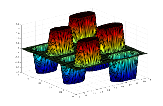
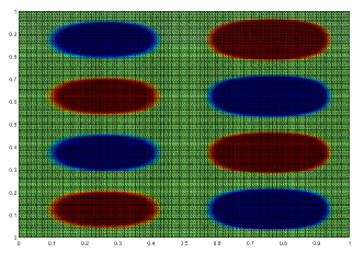
Figure 1: Optimal control $u_{h}$ on the square, $h=2^{-7}$. Dark red and dark blue areas correspond to $u_{h}=\pm 0.5$ and green areas to $u_{h}=0$

.

Example 2

(Stadler, , Example 1)

$$\left\{\begin{aligned} &\min\limits_{(y,u)\in Y\times U}\ \ J(y,u)=\frac{1}{2}\|y-y_{d}\|_{L^{2}(\Omega)}^{2}+\frac{\alpha}{2}\|u\|_{L^{2}(\Omega)}^{2}+{\beta}\|u\|_{L^{1}(\Omega)}\\ &\quad{\rm s.t.}\qquad-\Delta y=u,\quad\mathrm{in}\ \Omega=(0,1)\times(0,1)\\ &\qquad\qquad\qquad y=0,\quad\mathrm{on}\ \partial\Omega\\ &\qquad\qquad\qquad u\in U_{ad}=\{v(x)|a\leq v(x)\leq b,{\rm a.e}\ \mathrm{on}\ \Omega\},\end{aligned}\right.$$

where the desired state $y_{d}=\frac{1}{6}\sin(2\pi x)\exp(2x)\sin(2\pi y)$, the parameters $\alpha=10^{-5}$, $\beta=10^{-3}$, $a=-30$ and $b=30$. In addition, the exact solutions of the problem is unknown. Instead we use the numerical solutions computed on a grid with $h^{*}=2^{-10}$ as reference solutions.

An example for the discretized optimal control on mesh $h=2^{-7}$ is displayed in Figure 2. The error of the control $u$ w.r.t the $L^{2}$ norm with respect to the solution on the finest grid ($h^{*}=2^{-10}$) and the experimental order of convergence (EOC) for control are presented in Table 3. They confirms the linear rate of convergence w.r.t. $h$ as proved in Theorem 3.4 and Corollary 1.

Numerical results for the accuracy of solution, number of iterations and cpu time obtained by our ihADMM, classical ADMM and APG methods are also shown in Table 3. Experiment results show that the ADMM has evident advantage over the classical ADMM and the APG method in computing time. Furthermore, the numerical results in terms of iteration numbers also illustrate the mesh-independent performance of our ihADMM. In addition, in Table 4, we give the numerical results obtained by our two-phase strategy and the PDAS method with line search. As a result from Table 4, it can be observed that our two-phase strategy outperform the PDAS with line search in terms of the CPU time. These results demonstrate that our ihADMM is highly efficient in obtaining an approximate solution with moderate accuracy. And our two-phase strategy could represent an effective alternative to PDAS method.

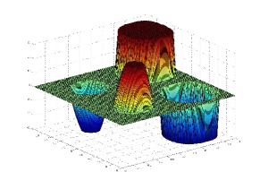
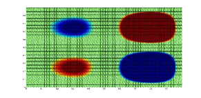
Figure 2: Optimal control $u_{h}$ on the square, $h=2^{-7}$. Dark red and dark blue areas correspond to $u_{h}=\pm 30$ and green areas to $u_{h}=0$

6 Concluding remarks

In this paper, elliptic PDE-constrained optimal control problems with $L^{1}$-control cost ($L^{1}$-EOCP) are considered. In order to make discretized problems have a decoupled form, instead of directly using the standard piecewise linear finite element to discretize the problem, we utilize nodal quadrature formulas to approximately discretize the $L^{1}$-norm and $L^{2}$-norm. It was proven that these approximation steps do not change the order of error estimates. By taking advantage of inherent structures of the problem, we proposed an inexact heterogeneous ADMM (ihADMM) to solve discretized problems. Furthermore, theoretical results on the global convergence as well as the iteration complexity results $o(1/k)$ for ihADMM were given. Moreover, in order to obtain more accurate solution, a two-phase strategy was introduced, in which the primal-dual active set (PDAS) method is used as a postprocessor of the ihADMM. Numerical results demonstrated the efficiency of our ihADMM and the two-phase strategy.

Table 1: Example 1: The convergence behavior of our ihADMM, classical ADMM and APG for ($\overline{\mathrm{DP}}_{h}$). In the table, $\#$dofs stands for the number of degrees of freedom for the control variable on each grid level.

$h$	$\#$dofs	$E_{2}$	EOC	Index	ihADMM	classical ADMM	APG
				iter	27	32	13
$2^{-3}$	49	0.3075	–	residual $\eta$	7.15e-07	7.55e-07	6.88e-07
				CPU time/s	0.19	0.23	0.18
				iter	31	44	13
$2^{-4}$	225	0.1237	1.3137	residual $\eta$	9.77e-07	9.91e-07	8.23e-07
				CPU times/s	0.37	0.66	0.32
				iter	31	58	12
$2^{-5}$	961	0.0516	1.2870	residual $\eta$	7.41e-07	8.11e-07	7.58e-07
				CPU time/s	1.02	2.32	1.00
				iter	32	76	14
$2^{-6}$	3969	0.0201	1.3112	residual $\eta$	7.26e-07	8.10e-07	7.88e-07
				CPU time/s	4.18	9.12	4.25
				iter	31	94	14
$2^{-7}$	16129	0.0078	1.3252	residual $\eta$	5.33e-07	7.85e-07	4.45e-07
				CPU time/s	17.72	65.82	26.25
				iter	32	127	13
$2^{-8}$	65025	0.0026	1.3772	residual $\eta$	6.88e-07	8.93e-07	7.47e-07
				CPU time/s	70.45	312.65	80.81
				iter	31	255	13
$2^{-9}$	261121	0.0009	1.4027	residual $\eta$	7.43e-07	7.96e-07	6.33e-07
				CPU time/s	525.28	4845.31	620.55

Table 2: Example 1: The convergence behavior of our two-phase strategy, PDAS with line search.

$h$	$\#$dofs	Index of performance	Two-Phase strategy		PDAS with line search
			ihADMM $+$ PDAS
		iter	13 $+$ 5		21
$2^{-3}$	49	residual $\eta$	8.55e-12		7.88e-12
		CPU time/s	0.17		0.32
		iter	13 $+$ 6		22
$2^{-4}$	225	residual $\eta$	1.24e-11		1.87e-11
		CPU times/s	0.27		0.54
		iter	14 $+$ 5		22
$2^{-5}$	961	residual $\eta$	8.10e-12		8.42e-12
		CPU time/s	0.95		2.07
		iter	14 $+$ 6		23
$2^{-6}$	3969	residual $\eta$	4.15e-12		4.00e-12
		CPU time/s	3.65		6.98
		iter	15 $+$ 6		23
$2^{-7}$	16129	residual $\eta$	1.43e-12		1.52e-12
		CPU time/s	22.10		43.13
		iter	15 $+$ 5		24
$2^{-8}$	65025	residual $\eta$	5.21e-12		5.03e-12
		CPU time/s	68.22		140.18
		iter	15 $+$ 6		24
$2^{-9}$	261121	residual $\eta$	3.77e-12		3.76e-12
		CPU time/s	540.57		1145.63

Table 3: Example 2: The convergence behavior of ihADMM, classical ADMM and APG for ($\overline{\mathrm{DP}}_{h}$).

$h$	$\#$dofs	$E_{2}$	EOC	Index	ihADMM	classical ADMM	APG
				iter	40	48	18
$2^{-3}$	49	0.3075	–	residual $\eta$	8.22e-07	8.65e-07	7.96e-07
				CPU time/s	0.30	0.51	0.24
				iter	41	56	18
$2^{-4}$	225	0.1237	1.3137	residual $\eta$	7.22e-07	8.01e-07	7.58e-07
				CPU times/s	0.45	0.71	0.44
				iter	40	69	19
$2^{-5}$	961	0.0516	1.2870	residual $\eta$	8.12e-07	8.01e-07	7.90e-07
				CPU time/s	1.60	3.05	1.58
				iter	42	85	18
$2^{-6}$	3969	0.0201	1.3112	residual $\eta$	6.11e-07	7.80e-07	6.45e-07
				CPU time/s	7.25	14.62	7.45
				iter	40	108	18
$2^{-7}$	16129	0.0078	1.3252	residual $\eta$	6.35e-07	7.11e-07	5.62e-07
				CPU time/s	33.85	101.36	34.39
				iter	41	132	19
$2^{-8}$	65025	0.0026	1.3772	residual $\eta$	7.55e-07	7.83e-07	7.57e-07
				CPU time/s	158.62	508.65	165.75
				iter	42	278	18
$2^{-9}$	261121	0.0009	1.4027	residual $\eta$	5.25e-07	5.56e-07	4.85e-07
				CPU time/s	1781.98	11788.52	1860.11
				iter	41	500	19
$2^{-10}$	1046529	–	1.4027	residual $\eta$	8.78e-07	Error	8.47e-07
				CPU time/s	42033.79	Error	44131.27

Table 4: Example 2: The behavior of two-phase strategy and the PDAS method.

$h$	$\#$dofs	Index of performance	Two-Phase strategy		PDAS with line search
			ihADMM $+$ PDAS
		iter	18 $+$ 8		24
$2^{-3}$	49	residual $\eta$	4.45e-12		4.36e-12
		CPU time/s	0.35		0.53
		iter	18 $+$ 8		25
$2^{-4}$	225	residual $\eta$	5.84e-12		6.01e-11
		CPU times/s	0.68		1.02
		iter	19 $+$ 7		24
$2^{-5}$	961	residual $\eta$	6.89e-12		6.87e-12
		CPU time/s	1.98		2.99
		iter	18 $+$ 8		26
$2^{-6}$	3969	residual $\eta$	2.15e-11		2.28e-11
		CPU time/s	8.42		12.63
		iter	19 $+$ 7		25
$2^{-7}$	16129	residual $\eta$	4.06e-11		3.88e-11
		CPU time/s	43.45		65.18
		iter	20 $+$ 8		25
$2^{-8}$	65025	residual $\eta$	8.45e-12		8.72e-12
		CPU time/s	189.04		283.20
		iter	20 $+$ 8		26
$2^{-9}$	261121	residual $\eta$	7.33e-12		7.21e-12
		CPU time/s	2155.01		3232.63
		iter	20 $+$ 8		26
$2^{-10}$	1046529	residual $\eta$	9.58e-12		9.73e-12
		CPU time/s	58049.57		87035.63

References

- (1) Z.-Z. Bai, M. Benzi, F. Chen, and Z.-Q. Wang, Preconditioned mhss iteration methods for a class of block two-by-two linear systems with applications to distributed control problems, IMA Journal of Numerical Analysis, 33 (2013), pp. 343–369.
- (2) A. Beck and M. Teboulle, A fast iterative shrinkage-thresholding algorithm for linear inverse problems, SIAM journal on imaging sciences, 2 (2009), pp. 183–202.
- (3) M. Bergounioux and K. Kunisch, Primal-dual strategy for state-constrained optimal control problems, Computational Optimization and Applications, 22 (2002), pp. 193–224.
- (4) T. Blumensath and M. E. Davies, Iterative thresholding for sparse approximations, Journal of Fourier Analysis and Applications, 14 (2008), pp. 629–654.
- (5) S. Boyd, N. Parikh, E. Chu, B. Peleato, and J. Eckstein, Distributed optimization and statistical learning via the alternating direction method of multipliers, Foundations and Trends® in Machine Learning, 3 (2011), pp. 1–122.
- (6) C. Carstensen, Quasi-interpolation and a posteriori error analysis in finite element methods, ESAIM: Mathematical Modelling and Numerical Analysis, 33 (1999), pp. 1187–1202.
- (7) E. Casas, R. Herzog, and G. Wachsmuth, Approximation of sparse controls in semilinear equations by piecewise linear functions, Numerische Mathematik, 122 (2012), pp. 645–669.
- (8) E. Casas, R. Herzog, and G. Wachsmuth, Optimality conditions and error analysis of semilinear elliptic control problems with cost functional, SIAM Journal on Optimization, 22 (2012), pp. 795–820.
- (9) L. Chen, ifem: an innovative finite element methods package in matlab, Preprint, University of Maryland, (2008).
- (10) L. Chen, D. Sun, and K.-C. Toh, An efficient inexact symmetric gauss–seidel based majorized admm for high-dimensional convex composite conic programming, Mathematical Programming, (2015), pp. 1–34.
- (11) J. C. de Los Reyes, C. Meyer, and B. Vexler, Finite element error analysis for state-constrained optimal control of the Stokes equations, WIAS, 2008.
- (12) O. L. Elvetun and B. F. Nielsen, The split bregman algorithm applied to pde-constrained optimization problems with total variation regularization, Computational Optimization and Applications, (2016), pp. 1–26.
- (13) M. Fazel, T. K. Pong, D. Sun, and P. Tseng, Hankel matrix rank minimization with applications to system identification and realization, SIAM Journal on Matrix Analysis and Applications, 34 (2013), pp. 946–977.
- (14) D. Gabay and B. Mercier, A dual algorithm for the solution of nonlinear variational problems via finite element approximation, Computers & Mathematics with Applications, 2 (1976), pp. 17–40.
- (15) R. Glowinski and A. Marroco, Sur l’approximation, par éléments finis d’ordre un, et la résolution, par pénalisation-dualité d’une classe de problèmes de dirichlet non linéaires, Revue française d’automatique, informatique, recherche opérationnelle. Analyse numérique, 9 (1975), pp. 41–76.
- (16) M. Hintermüller and M. Ulbrich, A mesh-independence result for semismooth newton methods, Mathematical Programming, 101 (2004), pp. 151–184.
- (17) K. Jiang, D. Sun, and K.-C. Toh, An inexact accelerated proximal gradient method for large scale linearly constrained convex sdp, SIAM Journal on Optimization, 22 (2012), pp. 1042–1064.
- (18) D. Kinderlehrer and G. Stampacchia, An introduction to variational inequalities and their applications, vol. 31, Siam, 1980.
- (19) X. Li, D. Sun, and K.-C. Toh, A schur complement based semi-proximal admm for convex quadratic conic programming and extensions, Mathematical Programming, 155 (2016), pp. 333–373.
- (20) M. K. Ng, F. Wang, and X. Yuan, Inexact alternating direction methods for image recovery, SIAM Journal on Scientific Computing, 33 (2011), pp. 1643–1668.
- (21) G. C. Philippe, The finite element method for elliptic problems, 1978.
- (22) T. Rees, H. S. Dollar, and A. J. Wathen, Optimal solvers for pde-constrained optimization, SIAM Journal on Scientific Computing, 32 (2010), pp. 271–298.
- (23) A. Schindele and A. Borzì, Proximal methods for elliptic optimal control problems with sparsity cost functional, Applied Mathematics, 7 (2016), p. 967.
- (24) G. Stadler, Elliptic optimal control problems with -control cost and applications for the placement of control devices, Computational Optimization and Applications, 44 (2009), pp. 159–181.
- (25) D. Sun, K.-C. Toh, and L. Yang, An efficient inexact abcd method for least squares semidefinite programming, SIAM Journal on Optimization, 26 (2016), pp. 1072–1100.
- (26) M. Ulbrich, Semismooth newton methods for operator equations in function spaces, SIAM Journal on Optimization, 13 (2002), pp. 805–841.
- (27) G. Wachsmuth and D. Wachsmuth, Convergence and regularization results for optimal control problems with sparsity functional, ESAIM: Control, Optimisation and Calculus of Variations, 17 (2011), pp. 858–886.
- (28) A. Wathen, Realistic eigenvalue bounds for the galerkin mass matrix, IMA Journal of Numerical Analysis, 7 (1987), pp. 449–457.
- (29) A. J. Wathen and T. Rees, Chebyshev semi-iteration in preconditioning for problems including the mass matrix, Electronic Transactions on Numerical Analysis, 34 (2009), p. S22.
- (30) H. Zhang and W. W. Hager, A nonmonotone line search technique and its application to unconstrained optimization, SIAM journal on Optimization, 14 (2004), pp. 1043–1056.