Mapping the three-dimensional dust extinction toward the supernova remnant S147 – the S147 dust cloud

Abstract

We present a three dimensional (3D) extinction analysis in the region toward the supernova remnant (SNR) S147 (G180.0–1.7) using multi-band photometric data from the Xuyi Schmidt Telescope Photometric Survey of the Galactic Anticentre (XSTPS-GAC), 2MASS and WISE. We isolate a previously unrecognised dust structure likely to be associated with SNR S147. The structure, which we term as “S147 dust cloud”, is estimated to have a distance $d=1.22\pm 0.21$ kpc, consistent with the conjecture that S147 is associated with pulsar PSR J0538 + 2817. The cloud includes several dense clumps of relatively high extinction that locate on the radio shell of S147 and coincide spatially with the CO and gamma-ray emission features. We conclude that the usage of CO measurements to trace the SNR associated MCs is unavoidably limited by the detection threshold, dust depletion, and the difficulty of distance estimates in the outer Galaxy. 3D dust extinction mapping may provide a better way to identify and study SNR-MC interactions.

1 Introduction

Supernova (SN) explosion is one of the most energetic events in a galaxy. It usually occurs near its maternal molecular cloud (MC). As such, MCs generally play a critical role in the evolution of the supernova remnants (SNRs). There are now $\sim$300 SNRs identified in our Milky Way (Green et al., 2014). About 70 of them are known to be or possibly be interacting with MCs (Jiang et al., 2010; Chen et al., 2014b). And SNR S147 (G180.0–1.7; hereafter referred to as S147), is claimed to be not one of those MC-interacting SNRs (Huang & Thaddeus, 1986; Jeong et al., 2012).

S147 is one of the most evolved SNRs in the Milky Way. It falls near the Galactic anticentre, at Right Ascension $\alpha$=05h39m00s and Declination $\delta=+7\degr 50^{\prime}0^{\prime\prime}$, and has a large angular size of about 200^′. It shows a complex network of long filaments in the optical (van den Bergh et al., 1973; Drew et al., 2005) and radio (Sofue et al., 1980; Kundu et al., 1980; Xiao et al., 2008) bands. The pulsar PSR J0538+2817, located near the center of S147, is suggested to be plausibly associated with S147 (Anderson et al., 1996; Ng et al., 2007). The pulsar is estimated to have an age of 3 $\pm$ 0.4 $\times$ 10⁴ yr (Kramer et al., 2003). X-ray emission has been detected from the pulsar by ROSAT All Sky Survey (Sun et al., 1996). In gamma-ray, an extended source is found to coincide with S147 (Katsuta et al., 2012). The $V$-band extinction of S147 is estimated to be $A_{V}$ = 0.7 $\pm$ 0.2 mag (Fesen et al., 1985) from optical spectroscopy. Dinçel et al. (2015) find that HD 37424, possibly the pre-supernova binary companion of the pulsar, has an extinction of $A_{V}$ = 1.28 $\pm$ 0.06 mag. The distance of S147 given in the literature varies between 0.6 and 1.6 kpc (Table 1). From the parallax of the pulsar, S147 is estimated to be at $1.30^{+0.22}_{-0.16}$ kpc (Chatterjee et al., 2009), more remote than estimated from the $\Sigma$-$D$ relation and by optical absorption analysis.

Table 1: An updated list of distance estimates for S147 based on Table 1 of Dinçel et al. (2015). (R^l) denotes the lower limit radius of the SNR.

Distance (kpc)	Method	Reference
1.6$\pm$0.3	$\Sigma-$D	Sofue et al. (1980)
0.8–1.37	Rl, $\Sigma-$D	Kundu et al. (1980)
0.6	Rl	Kirshner & Arnold (1979)
0.9	$\Sigma-$D	Clark & Caswell (1976)
0.8$\pm$0.1	$A_{V}$	Fesen et al. (1985)
1.06	$\Sigma-$D	Guseinov et al. (2004)
$<0.88$	High Vel Gas	Sallmen & Welsh (2004)
1.2	Pulsar DM	Kramer et al. (2003)
1.47${}^{+0.42}_{-0.27}$	Pulsar Plx	Ng et al. (2007)
1.3${}^{+0.22}_{-0.16}$	Pulsar Plx	Chatterjee et al. (2009)
1.333${}^{+0.113}_{-0.112}$	OB runaway star	Dinçel et al. (2015)
1.22$\pm$0.21	3D dust mapping	this work

Phillips et al. (1981) have detected low-velocity interstellar CO absorption features in the UV spectrum toward HD 36665 ($d$=0.9 kpc, once believed to lie behind S147). They claim that the SNR is evidently expanding into an inhomogeneous interstellar medium. Sallmen & Welsh (2004) have studied the interstellar Na i and Ca ii absorption lines in the high-resolution spectra of three stars at different distances in sight-lines towards S147. They find that two of the more distant stars, HD 36665 ($d$ = 880 pc) and HD 37318 ($d$ = 1380 pc), possess complex absorption features over intermediate velocities, while the nearest, foreground star, HD 37367 ($d$=360 pc), exhibits none of those features. Does S147 physically associated with any MCs? In general, a SNR-MC association is normally established with two types of study: 1) observation and detection of OH 1720 MHz masers (Frail et al., 1996; Green et al., 1997); and 2) sub-millimeter/millimeter molecular line and infrared emission line observation and analysis (Huang & Thaddeus, 1986; Jeong et al., 2012). Given the weakness of the maser emission, many more SNR-MC associations may yet remain to be revealed (Hewitt et al., 2009). In such cases, CO is a practical tracer of MCs commonly used to trace the SNR-MC interaction. Huang & Thaddeus (1986) present an early CO-line survey toward 26 outer Galactic SNRs with Galactic longitude $l$ between 70° and 210°. For S147, they do detect a weak cloud at a peak velocity around 4 km s^-1. They suggest that the cloud is probably in front of the SNR. Similarly, although a most recent CO survey for Galactic SNRs with $l$ between 60° and 190° by Jeong et al. (2012) also find some MCs at velocities between $\sim$ $-$14 and $+$5 $\rm km\,s^{-1}$, they believe none of those clouds are with the S147.

However, Katsuta et al. (2012) have reported a spatially extended gamma-ray source likely to be associated with SNR S147, suggesting possible interactions between the MCs and the SNR blast wave. The results of Huang & Thaddeus (1986) and Jeong et al. (2012) with regard to S147 are thus open to further discussion. In the direction of Galactic anti-center, the kinematic distance can hardly be determined from the local standard of rest (LSR) velocity, and thus be used to establish the possible association of a SNR with a MC. It is thus unclear whether the MCs found by Huang & Thaddeus (1986) and Jeong et al. (2012) are associated with S147 or not. In general, the strong CO $J=$1–0 emission is a good tracer of MCs. However the low density regions of a MC could be below the column density threshold required for a detection (Goodman et al., 2009; Chen et al., 2014a). There is also evidence that there is a substantial fraction of “dark” molecular gas not traced by CO emission (Planck Collaboration et al., 2011; Chen et al., 2015). In such cases, tracing the molecular gas using dust observation, in particular via the optical and/or the near-infrared dust extinction, seems to be a good, essential alternative way (Goodman et al., 2009). However, considering the traditional extinction maps lack the information of distance, obtaining distance-dependent three-dimensional (3D) extinction maps remains a challenge for this purpose.

With the availability of large amounts of multi-band photometric as well as spectroscopic data, thanks to a number of either already completed or still on-going large area or all-sky surveys, deriving 3D dust extinction maps for large sky areas has become an acknowledged aspect of Galactic studies that has received increasing attention in the recent years (Chen et al., 2013, 2014a; Schultheis et al., 2014; Green et al., 2015; Hanson et al., 2016). In this work, we improve the 3D dust mapping by Chen et al. (2014a) for the Galactic anticentre area and use the result to differentiate the foreground and background dust extinction of S147. The work reveals a large dust cloud, parts of which are possibly associated with S147, which we term as the “S147 dust cloud.” This paper is one of a series of three papers on the study of S147 based on the data of the Xuyi Schmidt Telescope photometric survey of the Galactic Anticentre (XSTPS-GAC, Liu et al. 2014; Zhang et al. 2013, 2014) as well as of the LAMOST spectroscopic Survey of the Galactic Anticentre (LSS-GAC, Liu et al. 2014, 2015). In the other two papers, we will present the S147 kinematics (Ren et al., in preparation), as well as the S147 dust properties including possible presence/absence of diffuse interstellar bands (DIBs) in the S147 dust cloud (Chen et al., in preparation).

In this paper, we first introduce our data set in Sect. 2. We describe in Sect. 3 our method to determine the extinction and distance of individual stars, as well as to derive the 3D dust extinction distribution. In Sect. 4 we present the results. We compare the morphology of the newly discovered S147 dust cloud with images of gas emissions from the radio to the gamma-ray in Sect. 5. We finish with Sect. 6 with the summary.

2 Data

Our work uses the optical photometry of the multi-band CCD photometric survey of the Galactic Anticentre with the Xuyi 1.04/1.20m Schmidt Telescope (XSTPS-GAC; Zhang et al. 2013, 2014; Liu et al. 2014). XSTPS-GAC collected data during the fall of 2009 and the spring of 2011, using the Xuyi 1.04/1.20 m Schmidt Telescope equipped with a 4k$\times$4k CCD camera, operated by the Near Earth Objects Research Group of the Purple Mountain Observatory. The survey took images in SDSS $g$, $r$ and $i$ bands. In total, XSTPS-GAC archives approximately 100 million stars down to a limiting magnitude of about 19 in $r$ band ($\sim$ 10$\sigma$). The astrometric accuracy is about 0.1^′′ and the global photometric accuracy is about 2 per cent (Liu et al., 2014). The total survey area of XSTPS-GAC is close to 7,000 deg², including an area of $\sim$ 5, 400 deg² centered on the Galactic anticentre, from $\alpha$ $\sim$ 3 to 9 h and $\delta$ $\sim~{}-$10° to $+60\degr$, an extension of about 900 deg² to the M31/M33 area and the bridging fields which connect the two areas.

The infrared photometry from the Two Micron All Sky Survey (2MASS; Skrutskie et al. 2006) and the Wide-field Infrared Survey Explorer (WISE; Wright et al. 2010) are also adopted in the work, in order to break the degeneracy between effective temperature (or intrinsic colours) and extinction (Berry et al., 2012; Chen et al., 2014a). 2MASS is an all-sky survey in $J$, $H$ and $K_{\rm s}$ bands, centered at 1.25, 1.65 and 2.16 $\mu$m, respectively. The survey was conducted with two 1.3-m telescopes located respectively at Mount Hopkins, Arizona and Cerro Tololo, Chile, in order to provide full coverage of both the northern and southern skies. For point-sources, the limiting magnitudes of 2MASS (S/N = 10) are approximately 15.8, 15.1 and 14.3 mag in $J$, $H$ and $K_{\rm s}$ respectively. The systematic photometric uncertainties of 2MASS are estimated to be smaller than 0.03 mag, while the astrometric uncertainties are less than 0.2^′′.

WISE is an all-sky survey in four infrared bands, $W1$, $W2$, $W3$ and $W4$, centered at 3.4, 4.6, 12 and 22 $\mu$m, respectively. The survey was conducted from a 40 cm telescope on board the satellite. Instead of the WISE All-Sky Release Catalog adopted by Chen et al. (2014a), in the current work we use the AllWISE Source Catalog which contains positions, proper motions, photometry and ancillary information of 748 million objects detected in the deep, coadded AllWISE Atlas Images (Kirkpatrick et al., 2014). The adopted AllWISE Source Catalog represents a significant improvement over the WISE All-Sky Release Catalog. It is significantly more sensitive in $W1$ and $W2$ bands, almost doubled, since all usable images from the whole WISE survey have been combined together. Furthermore, the AllWISE photometry is less biased and source astrometry is also improved. All sources in the AllWISE Source Catalogue have a measured S/N greater than 5 in at least one of the four bands. The AllWISE Source Catalog is 0.3–0.5 magnitudes fainter than the WISE All-Sky Release Catalog, with $95$ per cent source completeness at 17.1, 15.7, 11.7 and 7.7 mag in $W1$ to $W4$ band, respectively.

3 Method

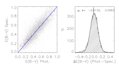
Figure 1: Comparisons of extinction values derived in the current work and recommended values presented in the LSS-GAC DR2 (Xiang et al., 2017b). The red pluses in the left panel represent median values in the individual bins. A blue straight line denoting complete equality is also overplotted to guide the eyes. In the right panel, the black curve is a Gaussian fit to the distribution of differences of values.

We select stars in a region centered at S147, between $177\degr\ <l<183\degr$ and $-5\degr\ <b<1\degr$. The determination of extinction for individual stars is similar as that of Chen et al. (2014a). Chen et al. (2014a) cross-matched the photometric catalogue of XSTPS-GAC with those of 2MASS and WISE, and applied spectral energy distribution (SED) fitting to the data. They obtained the best-fit values of extinction and distance for over 13 million stars and constructed a 3D extinction map of the Galactic anticentre. In the current work, we implement several improvements to the method of Chen et al. (2014a), described as follows.

1. In creating the library of standard stellar loci, Chen et al. (2014a) adopted the observed apparent colours of stars from their “high-quality reference sample of (essentially) zero extinction” directly. The extinction of those stars are indeed rather small ($A_{r}<0.075$ mag as given by the 2D map of Schlegel et al. 1998). Yet the reference stellar loci thus derived should still be slightly redder than they actually are. Consequently, the resultant extinction values may be slightly underestimated. Yuan et al. (2015) find that the $E(B-V)$ reddening values of Chen et al. (2014a) are systematically smaller than their values derived from spectroscopic data by about 0.06 mag. This systematical difference is partly caused by the usage of a stellar locus library that has not been corrected for reddening by Chen et al. (2014a). In the current work, we have dereddened stars in the “high-quality reference sample of (essentially) zero extinction” and recreated the library of standard stellar loci. The colour differences between the new stellar locus and the old ones are however found to be no larger than 0.01 mag on average.

2. Chen et al. (2014a) calculated extinction and distances of individual stars that are detected in all eight bands ($g,~{}r,~{}i,~{}J,~{}H,~{}K_{\rm s},~{}W1$ and $W2$). A large number ($\sim$ 10 per cent) of stars were consequently excluded as many of them were detected only in some of the infrared bands. In the current work, we have accepted all stars detected in all the three XSTPS-GAC optical bands ($g,~{}r,$ and $i$) and at least in any two infrared bands (2MASS $J,~{}H,$ and $K_{\rm s}$ or WISE $W1$ and $W2$). The new criteria enlarge the sample by 13 per cent.

Finally, we select stars with minimum $\chi^{2}<2$ and exclude those flagged as giant stars following the procedure of Chen et al. (2014a). This leads us to 161,642 stars with extinction values determined. The results are compared with those published in the second data release of value-added catalogue of LSS-GAC (LSS-GAC DR2; Xiang et al. 2017b). In LSS-GAC DR2, the “recommended” values of extinction were derived using the so-called “star pair” method (Yuan et al., 2015). We select from LSS-GAC DR2 stars with spectral signal to noise ratios (S/Ns) in blue band (4750Å) larger than 15 (‘snr_b’ $>15$) and unaffected by bright lunar light ( ‘moondis’ $>60$). In total there are 11,861 stars in common with the current sample. The comparison between our extinction values and those from Xiang et al. (2017b) is shown in Fig. 1. Our extinction values are in excellent agreement with the results from spectroscopic data. After corrected for the extinction of stars used to create the reference stellar loci, the systematic differences between our photometric extinction values and those based on spectroscopic analysis, are reduced to only about 0.01 mag, which is much lower than that found by Yuan et al. (2015; 0.06 mag) and thus can be entirely ignored. The differences have a dispersion just shy of 0.1 mag.

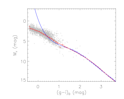
Figure 2: Photometric distance calibrated with the spectroscopic data. The grey dots show absolute magnitude $M_{r}$ versus intrinsic colour $(g-i)_{0}$ for the individual stars. The red pluses are median values of the individual bins. The blue curve represents the Ivezić et al. (2008) relation for metallicity [Fe/H]=$-$0.15 dex, and blue pluses mark selected values of the curve. The red curve is a 5-order polynomial fit of to red and blue pluses.

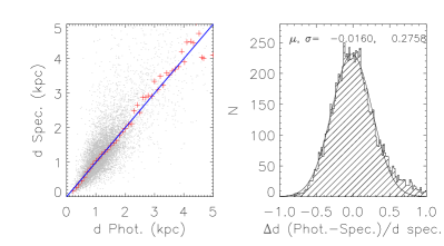
Figure 3: Comparison of distances derived in the current work and those from Xiang et al. (2017b). The red pluses in the left panel represent median values in the individual bins. A blue straight line denoting complete equality is overplotted to guide the eyes. In the right panel, the black curve is a Gaussian fit to the distribution of distance differences.

Chen et al. (2014a) calculated distances of the individual stars using the Ivezić et al. (2008) photometric parallax relation, assuming that all stars have a metallicity of [Fe/H] = $-$0.2 dex. Since the Ivezić et al. (2008) relation are based on globular clusters, which are usually of old ages, the relation may not be suitable for blue stars of young age of interest here. This effect is clearly visible in Fig. 3 of Chen et al. (2014a). In the case of young cluster, M35, its distance yielded by blue stars [$(g-i)_{0}<0.5$ mag] were clearly overestimated. Those blue young stars are still on the main sequence, while the Ivezić et al. (2008) relation is applicable only to stars of old ages (turnoff and sub-giant stars). In the current work, we solve this problem by recalibrating the photometric distance relation using the spectroscopic distances from LSS-GAC DR2 (Xiang et al., 2017b). Those spectroscopic distances are based on absolute magnitudes directly estimated from LAMOST spectra with the KPCA regression method using the LAMOST-Hipparcos training set (Xiang et al., 2017a). An obvious advantage of this approach is that absolute magnitudes thus estimated directly from LAMOST spectra are independent of any stellar model atmospheres and atmospheric parameters. The results are thus expected to suffer from minimal systematics. A comparison of the spectroscopic distances with the Gaia-TGAS parallaxes (Gaia Collaboration et al., 2016) shows that the typical uncertainties of thus deduced absolute magnitudes are only 0.3 mag for high quality spectra [$\rm S/N(4750\,\AA)$$>$ 50], corresponding to a distance error of 15 per cent (Xiang et al., 2017a).

To (re-)calibrate the photometric parallax relation using spectroscopic distances, we select stars from LSS-GAC DR2 using the criteria: ‘snr_b’ $>50$ for high blue band spectral S/Ns, log $g>3.8$ dex in order to exclude giant stars, and ‘moondis’ $>30$ for avoiding bright lunar light pollution. This yields 2,356 stars in common with our current sample. Absolute magnitudes in $r$-band $M_{r}$ of those stars from LSS-GAC DR2 are plotted against intrinsic colours $(g-i)_{0}$ from the current work. Also overplotted in the Figure is the Ivezić et al. (2008) relation assuming metallicity [Fe/H] = $-$0.15 dex. Since we have adopted a relatively high S/N cut, most of the stars are blue ones with a bright apparent magnitude. The Ivezić et al. (2008) relation seems to yield satisfactory results for stars redder than $(g-i)_{0}>0.5$ mag. For blue stars, the relation gives brighter absolute magnitudes than those from LSS-GAC DR2, leading to overestimated distances, as seen in the case of M35 in Chen et al. (2014a). To construct a new photometric parallax relation that is also valid for blue stars, a 5-order polynomial is used to fit $M_{r}$ as a function of $(g-i)_{0}$ colour, using the binned median values of spectroscopic absolute magnitudes from LSS-GAC DR2. Since only very few red stars are available from LSS-GAC DR2, stars of $(g-i)_{0}>1.5$ mag, we use simulated data for those redder colours created from the Ivezić et al. (2008) relation, assuming [Fe/H]=$-$0.15 dex. The fit yields,

$$M_{r} = 2.547+2.533(g-i)_{0}+1.546(g-i)_{0}^{2}$$ (1)

$$-1.578(g-i)_{0}^{3}+0.581(g-i)_{0}^{4}-0.0679(g-i)_{0}^{5}.$$

The relation is valid for stars over a wide colour range of $-$0.5 $<(g-i)_{0}<$ 3.7 mag. This relation is then applied to all star in our sample, with distances of the individual stars calculated using the standard relation,

$$d=10^{0.2(r-A_{r}-M_{r})+1}.$$ (2)

In Fig. 3 we compare the resultant distances with those from LSS-GAC DR2 for common stars of a LAMOST spectral $\rm S/N(4750\,\AA)$$>$ 15. Photometric distances from the newly constructed relation are in good agreement with the spectroscopic values. The differences are well fitted by a Gaussian. The systematic difference between our new photometric distances and those LSS-GAC spectroscopic values is only 1 per cent, with a dispersion of 28 per cent. Considering that uncertainties of spectroscopic distances for stars of a spectral $\rm S/N(4750\,\AA)$$>$ 20 are about 20 per cent (Xiang et al., 2017a), the uncertainties of the photometric distances derived in this work should also be about 20 per cent.

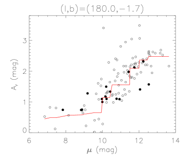
Figure 4: Mapping the 3D extinction for an example field at $(l,b)=(180.0\degr,-1.7\degr)$ of size 0.1° $\times$ 0.1°. The open and filled circles represent $r$-band extinction and distance values derived in the current work and those from LSS-GAC DR2, respectively. The red line shows the inferred maximum likelihood extinction as a function of distance.

With reddening values and distances deduced for individual stars in our sample, the 3D dust distribution toward S147 is then mapped. The procedure is similar to that of Green et al. (2014). We first divide our sample into subfields of size $6^{\prime}$ $\times$ $6^{\prime}$. This resolution is chosen to balance between high angular resolution and sufficient number of stars in each pixel (subfield) in order to obtain a robust extinction versus distance relation for the pixel. We have also tried alternative resolutions. For higher resolutions, a large fraction of pixels have not enough stars to obtain a robust extinction profile for the pixel. For lower resolutions, while we obtain similar results, some detailed features of the resultant dust distribution are washed out. For each pixel, we derive an $r$-band extinction profile $A_{r}(\mu)$, using the extinction values and distances thus obtained for individual stars, where $\mu$ is the distance module given by $\mu=5{\rm log}\,d-5$. We parameterise $A_{r}(\mu)$ by a piecewise linear function, given by,

$$A_{r}(\mu)=\Sigma_{0}^{\mu}(\Delta A^{i}_{r}),$$ (3)

where $\Delta A_{r}^{i}$ is the local extinction in each distance bin and $i$ the index of distance bin. The size of each distance bin is set to $\Delta\mu=0.5$ mag. A MCMC analysis is performed to find the best set of $\Delta A^{i}_{r}$ that maximises the likelihood defined as,

$$L=\Pi_{n=1}^{N}\frac{1}{2\pi\sigma_{n}}{\exp}(\frac{-(A^{n}_{r}-A^{n}_{r}(\mu))^{2}}{2\sigma^{2}_{n}}),$$ (4)

where $n$ is index of stars in the pixel, $A^{n}_{r}$ and $A^{n}_{r}(\mu)$ are respectively extinction derived in the current work and that simulated from Eq. (3) of the star, and $\sigma_{n}$ is the total uncertainty of the derived extinction and distance, given by $\sigma_{n}=\sqrt{\sigma^{2}(A_{r})+(A_{r}\frac{\sigma(d)}{d})^{2}}$ (Lallement et al., 2014). Note, however, that the error $A_{r}\frac{\sigma(d)}{d}$ resulting from the distance error is only an approximation for the assumption that the opacity is constant along the line of sight.

An example for the line of sight ($l,b$)=(180°, $-$1.7°), near the centre of S147, is shown in Fig. 4. There is little dust in distance bins of $\mu<10\,$mag. A sudden ‘jump’ in extinction, by about $1$ mag $A_{r}$, is clear visible at $\mu\sim 10$ mag, indicating the presence of a dust cloud at this distance. The extinction values and distances from LSS-GAC DR2 are also overplotted in the Figure as filled circles. They agree well with the extinction profile derived here.

4 The S147 dust cloud

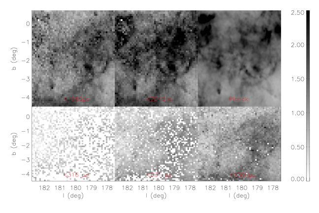
Figure 5: 2D extinction maps integrated to various distances in the direction of S147. X-axis denotes Galactic longitude while y-axis Galactic latitude. The distances, labelled in in each panel, increase from bottom left to top right. The top right panel shows the 2D extinction map from Planck Collaboration et al. (2014) for comparison.

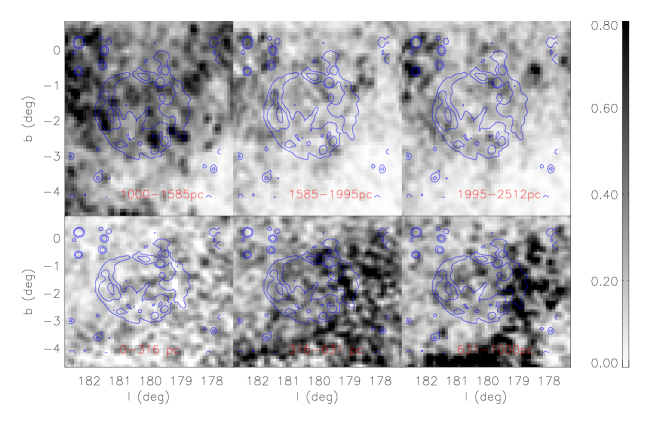
Figure 6: Distributions of dust extinction in individual distance bins in the direction of S147. The distance ranges of the bins are labelled in the individual panels. The x-axis denotes the Galactic longitude and the y-axis the Galactic latitude. The blue contours overplotted in all panels are total intensity map of 6 cm radio emission of ionised gas of S147 from Xiao et al. (2008).

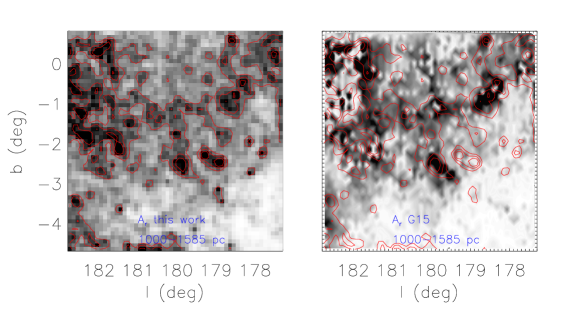
Figure 7: Distribution of dust extinction in the distance bin 1000 $<~{}d~{}<$ 1585 pc in the direction of S147 obtained in the current work (left panel) and that from Green et al. (2015, right panel). Red contours in each panel show the dust extinction distribution derived in the current work.

On the basis of the resulted reddening profiles of all pixels, we produce a 3D map of dust extinction in an area around S147, of $177.5\degr\ <l<182.5\degr$ and $-4.5\degr\ <b<0.5\degr$. To help visualise variations of dust extinction as a function of distance, we plot in Fig. 5 2D $r$-band extinction distributions integrated to selected distances from the Sun. In general, the extinction values increase with distances for all pixels, but the growth rates vary from pixel to pixel, suggesting highly inhomogeneous and clumpy dust distributions along the lines of sight. For the two maps of nearest distances ($d<$ 631 pc) plotted in Fig. 5, there are not enough stars for some of the pixels due to the limited volume and the bright saturation limit of XSTPS-GAC ($\sim 9$ mag). As one approaches a distances of 1.0 kpc, one encounters a large dust cloud of $l$ between 178° and 180°. This is parts of the Taurus-Perseus-Auriga cloud. At further distances ($d\lesssim$ 1.6 kpc), a structure of a significant amount dust is seen spatially coincident with S147. An addition dust cloud of $l$ around 182° and $b$ around 0° is then found at the furthest distances ($d\lesssim 2.5$ kpc). Finally, also plotted in Fig. 5 is the Planck 2D dust extinction map of the area, deduced from dust far-infrared thermal emission (Planck Collaboration et al., 2014), which can be compared with our map integrated to 2.5 kpc. Both maps show similar dust features, suggesting that the dust distribution obtained in the current work is robust.

To highlight dust features in different distance slices, we plot in Fig. 6 the distributions of dust extinction in distance bins $d<316$ pc, $316<d<631$ pc, $631<d<1000$ pc, $1000<d<1585$ pc, $1585<d<1995$ pc, and $1995<D<2512$ pc, respectively. For each distance bin, the extinction map has been smoothed with a Gaussian kernel of 0.3° full width at half maximum (FWHM). The maps reveal the fine structures of dust distribution in those distances bins. Also overplotted in blue contours of intensity flux of S147 at 6 cm radio wavelength (Xiao et al., 2008), delineating the distribution of ionised gas of S147. The dust seen spatially coincident with the ionised gas of S147 is distributed in distance bin $1000<d<1585$ pc, while the foreground dust of $l$ between 178° and 180° is located at distances $d<631$ pc and the background dust of $l$ around 182° and $b$ around 0° is located in bin $1995<d<2512$ pc. We note that although some features are seen in distance bin $631<d<1000$ pc, that may be attributed to the foreground dust cloud, they are actually artefacts caused by insufficient numbers of stars in some pixels at the selected spatial resolution of 0.1°. If one adopts a lower resolution, such as 0.2°, one sees the foreground dust falls entirely $d<631$ pc.

There is a large dust cloud at distances between $1000<d<1585$ pc in the direction of S147. Within the 6cm emission area of S147, parts of the dust cloud, which has a morphology spatially coincident with the ionised gas of S147, are referred to as the “S147 dust cloud”. There are three dense clumps of relatively high extinction ($\Delta A_{r}$ $\sim$ 1 mag) in S147 dust cloud, which are located on the radio shell of S147, respectively at $l~{}\sim$ 181.3° and $b~{}\sim~{}-$2.2°, $l~{}\sim$ 179.9° and $b~{}\sim~{}-$2.7° and $l~{}\sim$ 179.0° and $b~{}\sim~{}-$2.5°. In Fig. 7 we compare our derived dust distribution at distances between $1000<d<1585$ pc to that of Green et al. (2015), who present a 3D map of the interstellar dust reddening deduced using the Pan-STARRS 1 and 2MASS photometry. Values of $E(B-V)$ of Green et al. (2015) are converted to $A_{r}$ using the coefficient given by Schlafly & Finkbeiner (2011). In general, the agreement is good. The morphology of the S147 dust cloud derived here shows quite similar features as that of Green et al. (2015), except for the dense clump at $l~{}\sim$ 179.0° and $b~{}\sim~{}-$2.5°. This clump could be parts of the foreground dust cloud that has been wrongly placed at an artificially larger distance due to the uncertainties in distance estimation and the insufficient numbers of stars in those pixels (See also in Fig. 9). A detailed examination of the S147 dust cloud, including a precise estimate of its distance as well as of mass, is presented below.

4.1 Distance

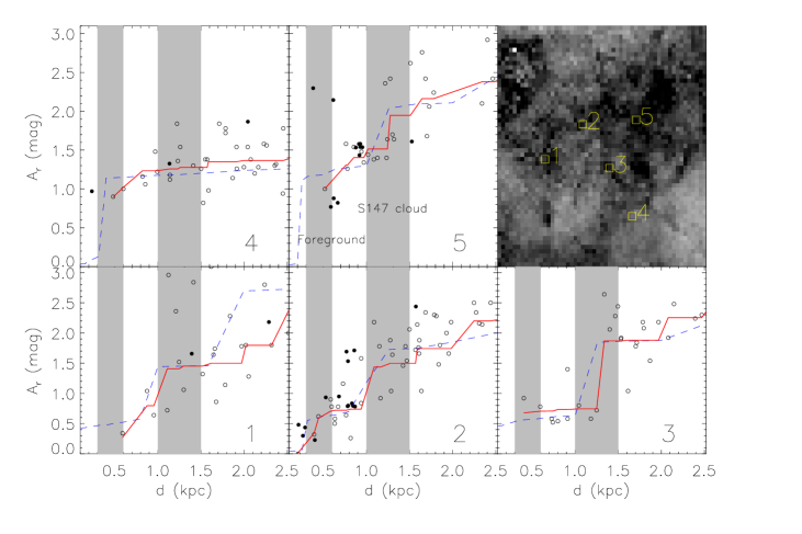
Figure 8: Extinction values as a function of distance of stars in five select lines of sight. Our extinction map integrated to 2.5 kpc is shown in the top-right panel, with the selected lines of sight marked. The grey scale corresponds to a 0–2.5 mag range of extinction in $r$-band, $A_{r}$. The other five panels, marked by the number of sight line 1 to 5, show values of extinction as a function of distance for stars within the $0.1\degr\times 0.1\degr$ pixel area of the sightline. The open and filled circles correspond to stars in our current sample and those available from LSS-GAC DR2, respectively. The vertical shadows delineate the distance ranges of the foreground dust cloud at about 0.5 kpc and the S147 cloud at about 1.2 kpc. The red solid lines are best-fit extinction-distance relations to the data, while the blue dashed lines are corresponding relations from Green et al. (2015).

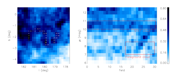
Figure 9: Distributions of dust extinction as a function of distance for subfields of the S147 dust cloud. The left panel shows the distribution of dust in distance bin from 1000 to 1585 pc. The map has a resolution of 0.2°. The selected pixels belonging to the S147 dust cloud are used for a precise analysis of distance to the cloud, are labelled with a unique number from 1 to 30. Each pixel is of size $0.2\degr\ \times 0.2\degr$. The right panel shows the amounts of extinction $A_{r}$ for the 30 pixels (subfields) in different distance bins. The X-axis denotes the unique number of the pixel. The red squares mark roughly the boundaries of pixels belonging to the foreground cloud and the S147 dust cloud, respectively.

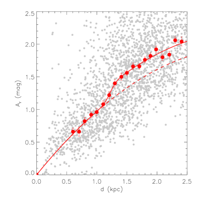
Figure 10: Extinction values plotted against distances for stars in the selected subfields No. 1 to 22 (Fig. 9). The red circles are median values in the individual distance bins starting from 0.5 kpc. The errorbars are the standard errors. The red solid line is the best-fit extinction law based on the median values. The red dashed line is the modeled extinction law without the contribution of the S147 dust cloud.

From the above 3D dust maps, it is easy to infer that the S147 dust cloud has a distance between 1.0 and 1.6 kpc. The accuracy of this inferred distance is limited by uncertainties of distances of individual stars. The uncertainties of distances of individual stars, which are estimated to be 20 per cent, arise from uncertainties in measured colours of the stars, in constructed library of stellar loci, as well as from uncertainties in the distribution of stellar ages and metallicities. Our distance resolution is also limited by pixel size of $6^{\prime}\times 6^{\prime}$ used to fit the 3D dust distribution profiles. A better approach to estimate the distance of the S147 dust cloud is to use larger pixels with a single, common dust distribution profile, similar to the technique adopted by Schlafly et al. (2014) for the estimation of distances to MCs. However, one should note that when Schlafly et al. (2014) used this technique to estimate distances to MCs, they assumed that the dust extinction is dominated by a single cloud. This is not true in our case. In Fig. 8 we plot the distributions of $r$-band extinction values as a function of distance for stars in five representative pixels (subfields) toward S147. Also overplotted in the Figure are the best-fit extinction and distance relations for those lines of sight from Green et al. (2015). Green et al. (2015) obtain their 3D dust distribution based on the Pan-STARRS 1 (PS1; Kaiser et al. 2002) and 2MASS photometry. The map has a resolution of about 5^′ in the area of interest here. For each line of sight, their best fit reddening and distance relation nearest to the pixel is used. Their reddening values are converted to $r$-band extinction assuming $A_{r}=2.32E(B-V)$ (Yuan et al., 2013). In general, our deduced extinction profiles are in good agreement with those of Green et al. (2015), except that at large distances ($d$ $>$ 1.5 kpc), Green et al. (2015) obtain higher extinction than ours. This is mainly due to the higher angular resolution of their map and deeper photometry used. Extinction values and distances available from LSS-GAC DR2 are also plotted in the Figure. Again the extinction profiles derived here match the spectroscopic results well. The vertical shadows overplotted in Fig. 8 delineate respectively the distance ranges of the foreground cloud (300$<d<$600 kpc) and of the S147 cloud (1000$<d<$1500 kpc). A precise distance estimate for the foreground cloud is difficult given that there is not enough stars in front of the dust in our sample, due to the bright saturation limit of XSTPS-GAC and the high angular resolution of the extinction map adopted here. In Fig. 8, the best fit extinction profiles (red lines in the individual panels) of the selected lines of sight No. 1, 2 and 3 have a “jump” in extinction value at a distance between 1000 and 1500 pc. It is not surprising to see some variations in “jump” distances for different pixels, given a pixel size of only 0.1° $\times$ 0.1° and a bin size of distance module of 0.5 mag (about 300 pc at 1000 pc). For line of sight No. 4, only a “jump” in extinction attributed to the foreground cloud is seen. For line of sight No. 5, two “jumps” are visible, produced by the foreground and the S147 cloud, respectively.

In Fig. 9 we investigate possible variations in distance of different portion of the S147 dust cloud. For this purpose, we have repeated the 3D dust mapping procedure with a lower resolution of 0.2°. The narrow filamentary features and the individual small clumps become poorly resolved at this resolution, but the resultant map of dust distribution is qualitatively similar. We then select pixels belonging to the S147 dust cloud and investigate the amounts of dust extinction of those pixels in different distances bins. Thirty pixels are selected at Galactic longitudes between 178° and 182°  running through the entire cloud and labelled by a number from 1 to 30. The amounts of extinction of these pixels are shown in Fig. 9. The maps have been smoothed with a Gaussian kernel of 0.5° FWHM for better illustration. The S147 dust cloud appears prominently in Fig. 9 as a dark blue snake at distance modulus $10<\mu<11$ mag, i.e. of distances $1.0<d<1.5$ kpc, for all the pixels. Contamination from the foreground cloud is also apparent in pixels of number 23 to 30.

Finally, we select all stars in the fields labelled from No. 1 to 22. The above analysis shows that the extinction observed in those regions are mainly contributed by a single cloud, i.e. the S147 cloud. The variations of extinction as a function of distance of all stars in these pixels are plotted in Fig. 10. The scatter of extinction values at a given distance of these stars is large. And this may be attributed to the fact that the stars cover a large area (nearly 1 deg²). Yet via the binned median extinction values, one can clearly see the extinction “jump” produced by the S147 dust cloud at a distance between 1100 and 1300 pc. A simple extinction model is applied to estimate the distance and amplitude of the “jump”. We assume a extinction-distance relation as following,

$$A_{r}(d)=A_{r}^{0}(d)+A_{r}^{1}(d),$$ (5)

where $A_{r}^{1}(d)$ is the contribution of extinction from the S147 cloud, i.e. the “jump” component. We assume that this component can be simply described by a Gaussian function. Thus the integrated extinction contributed the S147 cloud to a distance $d$ is given by,

$$A_{r}^{1}(d)=\frac{\delta A_{r}}{2}{\rm erf}(\frac{d-d_{0}}{\sqrt{2}*\delta d}),$$ (6)

where $\delta A_{r}$ is the extinction “jump” amplitude, $\delta d$ is the width of the cloud and $d_{0}$ is the distance of peak extinction (i.e. the centre of the S147 dust cloud). In Eq. (5), $A_{r}^{0}$ represents the smooth extinction component contributed by the general interstellar medium and is assume to be a 2-order polynomial (Chen et al., 1998),

$$A_{r}^{0}(d)=ad+bd^{2},$$ (7)

where $a$ and $b$ are polynomial coefficients. The binned average extinction values for the distance range $0.6<d<2.5$ kpc are fitted with the extinction model described above using a maximum likelihood method. The best-fit result is overplotted in Fig. 10. The fit yields $\delta A_{r}=0.24\pm 0.28$ mag, $\delta d$=81$\pm 299$ pc and $d_{0}$=1223$\pm 206$ pc. This distance to the S147 dust cloud yielded by our analysis, $d=$1.22$\pm$0.21 kpc, is consistent with the most recent distance estimates of S147, either based on the plausible association of S147 with pulsar PSR J0538 + 2817 (Kramer et al., 2003; Ng et al., 2007; Chatterjee et al., 2009) or its pre-supernova binary companion HD 37424 (Dinçel et al. 2015, see Table 1). The latest estimate of distance to the pulsar is 1.30${}^{+0.22}_{-0.16}$ kpc, based on the parallax measurement of the pulsar (Chatterjee et al., 2009), while that based on its pre-supernova binary companion is 1.333${}^{+0.103}_{-0.112}$ kpc (Dinçel et al., 2015). Both results are in good agreement with our estimate of distance to the S147 dust cloud. The shorter distance, $d<$ 0.88 kpc, obtained via an absorption line analysis of the B1e star HD 36665 (which is assumed to be formed out of the gas associated with S147; Phillips et al. 1981; Sallmen & Welsh 2004), may be caused by the contamination of the foreground cloud. Gas detected in the absorption line spectrum of HD 36665 might in fact originated from the foreground cloud, which is estimated to have a distance $d<631$ pc.

From the above model, the integrated dust extinction toward the S147 dust cloud is $A_{r}=1.26$ mag ($A_{V}=1.48$ mag). We note however there are significant variations in the total extinction across the surface of the cloud. Former extinction estimates of S147, $A_{V}=1.28$ mag by Dinçel et al. (2015) and $A_{V}=0.7$ mag by Fesen et al. (1985), are both based on observation of a small area of the cloud. The above best-fit model also yields $\delta A_{r}=0.24\pm 0.28$ mag, representing the average extinction contributed by the cloud. For some parts of the cloud, such as the three dense clumps mentioned above, the total extinction could be as large as $\delta A_{r}\sim 1$ mag.

4.2 Mass

The mass of the S147 dust cloud is dominated by atomic and molecular hydrogen. We can make a rough estimate of the mass of the cloud by converting the observed extinction $A_{V}$ to mass. Following Lombardi et al. (2011) and Schlafly et al. (2015), the total mass $M$ of the cloud is given by,

$$M=\frac{d^{2}\mu}{DGR}\int{A_{V}(\Omega)d\Omega}$$ (8)

where $d$ is the distance to the cloud, $\mu$ the mean molecular weight, $A_{V}({\Omega})$ the optical extinction $A_{V}$ in solid angle ${\Omega}$, and $DGR$ is the dust-to-gas ratio,

$$DGR=A_{V}/N({\rm H}),$$ (9)

where $N({\rm H})=N({\rm H~{}{\scriptstyle I}})+2N({\rm H_{2}})$ is the total hydrogen column density. We convert our $r$-band extinction to $V$-band using the extinction law of Yuan et al. (2013), which yields $A_{V}=1.17A_{r}$. We adopt $\mu=1.37$ from Lombardi et al. (2011) and $DGR=4.15\times 10^{-22}~{}\mathrm{mag}~{}\mathrm{cm}^{2}$ from Chen et al. (2015). The boundary of the S147 cloud is defined as $178.6\degr\leq l\leq 182.0\degr;$ and $-3.2\degr\leq b\leq 0\degr$. We assume that only dust within distance range 1000 $<d<$ 1585 pc is associated with S147, and the dust is distributed as a thin screen at a distance of $d$=1.2 kpc.

This leads to a total mass of the S147 cloud of 176,315$M_{\odot}$. The estimate is certainly quite rough, considering the many simplifications involved. The accuracy is mainly limited to the uncertainties of adopted distance. In the analysis we have assumed a distance of 1.2 kpc. The uncertainty in the distance could easy make the estimated mass to change by a factor of two. Moreover, due to the uncertainty in distance estimate, some of the dust actually belonging to the foreground or background medium could be wrongly attributed to the S147 dust cloud, or vice versa. In the current calculation, we have accepted all dust in a large range of estimated distances, 1000 $<d<$ 1585 pc, as belong to the S147 cloud. Considering that in the case of S147, there is significant dust presence both in the foreground and background, some contamination from the foreground and background material is somehow inevitable. Thus the total mass obtained above could be overestimated. The choice of $DGR$ value may also lead to additional uncertainties. The most cited value, $5.3\times 10^{-22}~{}\mathrm{mag}~{}\mathrm{cm}^{2}$, derived by Bohlin et al. (1978) is slightly larger than the adopted value here. Chen et al. (2015) find that the values of $DGR$ for the individual clouds in the Galactic anticentre can vary by a factor of two. In spite of all of these uncertainties, the analysis here still place some useful constraints on the mass of the S147 dust cloud. The estimated mass, approximately 10⁵ $M_{\odot}$, is however of the same order of magnitude of those estimates for the well known molecular clouds like Orion, Monoceros R2, Rosette and the Canis Major (Lombardi et al., 2011).

5 Morphology of the S147 dust cloud

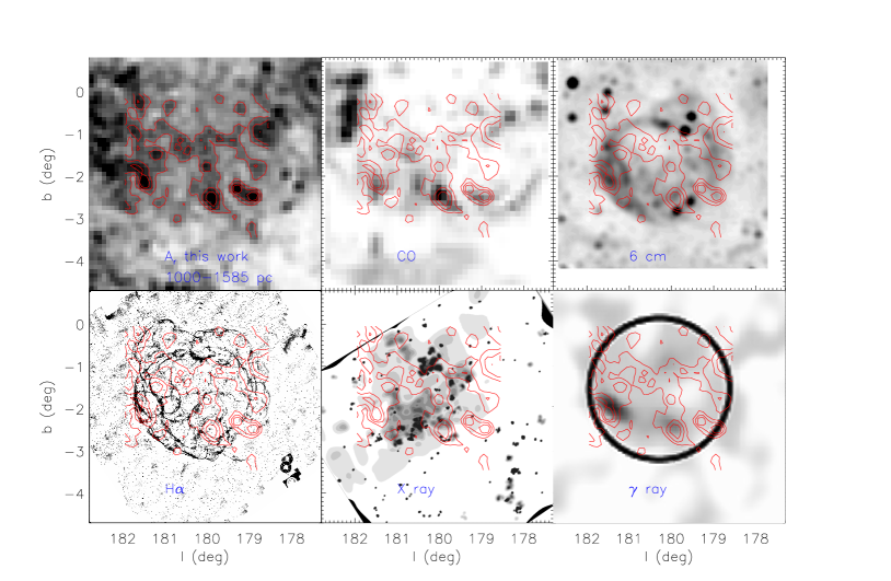
Figure 11: The extinction distribution of S147 dust cloud is compared to millimetre CO, radio 6 cm continuum, optical $\mathrm{H\alpha}$, X-ray, and gamma-ray emission maps of the region of interest. The data used are: CO from Dame et al. (2001), radio 6 cm from Xiao et al. (2008), $\mathrm{H\alpha}$  from Drew et al. (2005), X-ray from ROSAT (Voges et al., 1999) for the energy range 0.4 – 0.9 keV, and gamma-ray from Katsuta et al. (2012). The black circle in the last panel marks S147. The red contours in each panel shows the dust extinction distribution of the S147 dust cloud.

In this section, we compare the morphology of the newly identified S147 dust cloud to maps of S147 viewed in other frequencies, in order to investigate the plausible correlation between the dust and other tracers, such as cool or hot gas, in the region of interest. The comparisons is presented in Fig. 11, where we compare the dust extinction distribution to the S147 images in millimetre from the CO, 6 cm radio continuum , optical $\mathrm{H\alpha}$, X-ray and gamma-ray emission, respectively.

5.1 CO emission

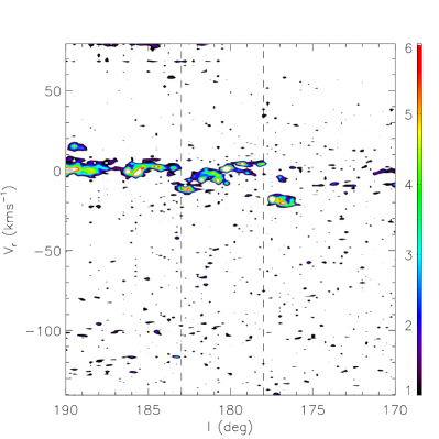
Figure 12: Galactic longitude and velocity diagram of CO gas from Dame et al. (2001) for the region of $-3\degr\ <b<-1\degr$. The vertical dashed lines mark the longitude range of the S147 dust cloud.

The second panel of Fig. 11 shows the CO emission map from Dame et al. (2001) in the region of interest. Dame et al. (2001) combine large-scale CO surveys of the Galactic plane and of all large local clouds at higher latitudes into a composite map of the entire Milky Way at an angular resolution ranging from 9^′ to 18^′. The panel shows the total CO column density in the area, with contours of the S147 dust cloud overplotted. Most prominent features including the three dense clumps seen in the dust map are clearly detected in CO emission. On the other hand, regions of less dust extinction have no detectable CO, presumably as a result of the low column density of dust grains in those regions. CO molecules have been be largely photodissociated due to insufficient shielding.

Huang & Thaddeus (1986) carried out a CO survey toward all SNRs from Galactic longitude 70° to 210°. They find two large MCs, coincident in position with the three dense dust clumps of S147 found here. Recently, Jeong et al. (2012) carried out a CO survey of SNRs between longitudes 70° – 190° using the Seoul Radio Astronomy Observatory (SRAO) 6-m radio telescope. They have also found some molecular clouds, at velocities ranging from $\sim$  $-$14 to $+$5 $\rm km\,s^{-1}$, that overlap in position with the dense dust regions of S147. Both studies point out that the MCs detected do not show features correlated with the S147 SNR. This may be partly caused by the lack of distance information. Also, one should bear in mind that the CO ($J~{}=$ 1 – 0) may not be a good tracer for the diffused gas of low dust column densities. The 3D dust mapping technique employed here not only allows us to measure a distance to the S147 dust cloud, but also uncover the diffuse parts of the cloud. We believe that 3D dust extinction could be a better tracer to trace the SNR associated MCs than the CO ($J~{}=$ 1 – 0) emission.

Fig. 12 shows the observed CO (Dame et al., 2001) distribution in the direction of Galactic anticentre within $-3\degr<b<-1\degr$ in the $l$ and $V_{r}$ space. The black lines in the Figure enclose the feature of the S147 dust cloud. The velocity of the cloud spans from $-$10 to 5 $\rm km\,s^{-1}$, in consistent with the observation of Huang & Thaddeus (1986) and Jeong et al. (2012). The peak velocities in regions of smaller Galactic longitudes are slightly higher than those of higher Galactic longitudes. In particular, for the clouds of $l<$180°, the radial velocities of CO emitting gas are positive, while of $l>$180° are negative. This could be explained by the expansion of the cloud. Consequently, the variations seen in velocity does not clearly correlate with the variations observed in distance. In principle, observation of neutral hydrogen atoms should be sensitive enough to trace the gas associated with the dust cloud, especially for regions lacking strong CO emission. Unfortunately, in the region of S147, any $\rm H~{}{\scriptstyle I}$ emission associated with the cloud is lost in strong background of the Galactic $\rm H~{}{\scriptstyle I}$ disk. It could be a challenge to isolate the clumps and filaments correlated with the dust cloud found in the current work.

5.2 6 cm radio emission

The third panel of Fig. 11 shows the radio 6 cm map of S147 (Xiao et al., 2008). The map gives the total intensity of radio continuum of S147 at 6 cm (4800 MHz), obtained with the Urumqi 25-m telescope between January 2005 and February 2006. It has an angular resolution of 9.51^′. Again overplotted in the panel is the $r$-band extinction contours of the S147 dust cloud. The 6 cm map shows a spherical SNR shell with a hollow region at the centre, quite different from the morphology of dust distribution. Although one does not expect any good correlation between the dust extinction and the emission of ionised gas as traced by the 6 cm observation, one does see some level of correlation between them in the Figure. At the locations of two out of three dense clumps of the S147 dust cloud (one at $l~{}\sim$ 181.3°, $b~{}\sim~{}-$2.2°  and another at $l~{}\sim$ 179.9°, $b~{}\sim~{}-$2.7°), the 6 cm emission is also strong.

5.3 $\mathrm{H\alpha}$ emission

The fourth panel of Fig. 11 shows the $\mathrm{H\alpha}$ image of S147 from the INT Photometric $\mathrm{H\alpha}$ Survey of the Northern Galactic Plane (IPHAS; Drew et al. 2005). The $\mathrm{H\alpha}$ image shows beautiful ring-like filaments and has similar features as the 6 cm map. Like the 6 cm map, the $\mathrm{H\alpha}$ image shows complicated spatial correlations with the dust cloud we found in this paper. A detailed kinematic analysis of the optical filaments and shells will be presented in a separate work (Ren et al., in preparation).

5.4 X-ray emission

Supernova remnants often emit strong X-ray emission. Sauvageot et al. (1990) report that no X-ray emission is observed from S147 with the X-ray satellite EXOSAT. Sun et al. (1996) claim that X-ray emission from S147 has been unambiguously detected in the ROSAT all-sky survey. In the fifth panel of Fig. 11 we show the X-ray image in the energy range of 0.4 – 0.9 keV from the ROSAT all sky survey (Voges et al., 1999) for the region of interest. The X-ray image has a patchy appearance without a clear shell, with some similarity with the 6 cm image. There is anti-correlation between the X-ray emission and the dust extinction. In regions where the X-ray emission is strong, the extinction is relative low, and vice versa. This is mainly due to the fact that the dust cloud may have absorbed all the low-energy X-rays produced behind it.

5.5 Gamma-ray emission

Finally we show in Fig. 11 the gamma-ray image of S147 (Katsuta et al., 2012). Katsuta et al. (2012) have analysed the gamma-ray data obtained with the Large Area Telescope on board the Fermi Gamma-ray Space Telescope (Atwood et al., 2009) in the region toward S147. They create a background-subtracted count map of the region above 1 GeV (showed in the right panel of Fig. 1 of Katsuta et al. 2012), which is reproduced here. There is spatially extended gamma-ray emission of energy range 0.2–10 GeV in the region. Two of the prominent dense dust clumps centred at ($l$, $b$) = (181.3°, $-2.2$°) and ($l$, $b$) = (179.9°, $-$0.4°) spatially coincident with the gamma-ray emission.

The gamma-ray emission surrounding the SNR is expected to be primarily emitted via the pion decay produced by the interaction between CR protons and dense medium (p-p interaction), while the leptonic origin is unlikely for such an old SNR (Aharonian et al., 1994; Ackermann et al., 2013). The morphology correspondence between hadronic gamma-ray emission and MC has been found in a number of evolved SNR (e.g., W44, IC443; Seta et al. 1998). The comparisons of gamma-ray emission and dust distribution in the direction of S147 as presented above shows a possible correlation between them, suggesting probable interactions between S147 and its surrounding MCs (Katsuta et al., 2012). Finally, Katsuta et al. (2012) model the gamma-ray spectrum of S147 and obtain a gas density between 100 – 500 cm^-3, corresponding to a dust cloud of extinction $A_{V}$ $\sim$ 0 – 1 mag. This is consistent with the estimate of extinction of the S147 cloud obtained in this paper.

6 Conclusion

In this work, we present a 3D map of dust extinction toward the SNR S147. When integrated to a distance of about 2.5 kpc, our map traces similar dust features as revealed by the Planck data. We have estimated distances to the several dust clouds detected in the map. The work reveals a large dust cloud at a distance between 1 $<~{}d~{}<$ 1.5 kpc. Parts of the cloud are possibly associated with the SNR, and are termed as the “S147 dust cloud.” The cloud is consistent of several dense clumps of high extinction, which locate on the radio shell of S147, as well as some diffuse parts of low extinction. We estimate the distance to the cloud using a simple extinction model. This yields a distance of 1.22$\pm$0.21 kpc, in consistent with the distance estimated for the SNR. We have also obtained a rough estimate of the mass of the S147 dust cloud, which is about 10⁵ $\rm M_{\odot}$.

We compare the dust extinction distribution of the S147 dust cloud with the images of S147 in other frequencies, including those in the CO, radio 6 cm, $\mathrm{H\alpha}$, X-ray and gamma-ray emission. The dust distribution is not surprisingly correlated with the CO emission. More interestingly, the dust distribution is spatially correlated with the gamma-ray emission in energy range 0.2 – 10 GeV, indicating that the dust cloud is possibly associated with the SNR and has complicated interactions with the SNR.

We conclude that comparing to the CO ($J$=1–0) emission, 3D dust mapping could be a viable technique to search for MCs associated with SNRs, and to study the SNR-MC interactions. In a future work, we will present a systematic survey of MCs associated with SNRs in the outer disk of the Galaxy (Yu et al., in preparation). Utilizing tens of thousands of stellar spectra collected as parts of LSS-GAC survey in the vicinity of S147, we are able to study the extinction law, referring the dust size distribution, as well as to carry out a demographic study of the DIBs of the S147 dust cloud. A related work on these lines will be presented in near future (Chen et al., in preparation).

References

- Ackermann et al. (2013) Ackermann, M., et al. 2013, Science, 339, 807
- Aharonian et al. (1994) Aharonian, F. A., Drury, L. O., & Voelk, H. J. 1994, A&A, 285, 645
- Anderson et al. (1996) Anderson, S. B., Cadwell, B. J., Jacoby, B. A., Wolszczan, A., Foster, R. S., & Kramer, M. 1996, ApJ, 468, L55
- Atwood et al. (2009) Atwood, W. B., et al. 2009, ApJ, 697, 1071
- Berry et al. (2012) Berry, M., et al. 2012, ApJ, 757, 166
- Bohlin et al. (1978) Bohlin, R. C., Savage, B. D., & Drake, J. F. 1978, ApJ, 224, 132
- Chatterjee et al. (2009) Chatterjee, S., et al. 2009, ApJ, 698, 250
- Chen et al. (1998) Chen, B., Vergely, J. L., Valette, B., & Carraro, G. 1998, A&A, 336, 137
- Chen et al. (2015) Chen, B.-Q., Liu, X.-W., Yuan, H.-B., Huang, Y., & Xiang, M.-S. 2015, MNRAS, 448, 2187
- Chen et al. (2014a) Chen, B.-Q., et al. 2014a, MNRAS, 443, 1192
- Chen et al. (2013) Chen, B. Q., Schultheis, M., Jiang, B. W., Gonzalez, O. A., Robin, A. C., Rejkuba, M., & Minniti, D. 2013, A&A, 550, A42
- Chen et al. (2014b) Chen, Y., Jiang, B., Zhou, P., Su, Y., Zhou, X., Li, H., & Zhang, X. 2014b, in IAU Symposium, Vol. 296, Supernova Environmental Impacts, ed. A. Ray & R. A. McCray, 170–177
- Clark & Caswell (1976) Clark, D. H. & Caswell, J. L. 1976, MNRAS, 174, 267
- Dame et al. (2001) Dame, T. M., Hartmann, D., & Thaddeus, P. 2001, ApJ, 547, 792
- Dinçel et al. (2015) Dinçel, B., Neuhäuser, R., Yerli, S. K., Ankay, A., Tetzlaff, N., Torres, G., & Mugrauer, M. 2015, MNRAS, 448, 3196
- Drew et al. (2005) Drew, J. E., et al. 2005, MNRAS, 362, 753
- Fesen et al. (1985) Fesen, R. A., Blair, W. P., & Kirshner, R. P. 1985, ApJ, 292, 29
- Frail et al. (1996) Frail, D. A., Goss, W. M., Reynoso, E. M., Giacani, E. B., Green, A. J., & Otrupcek, R. 1996, AJ, 111, 1651
- Gaia Collaboration et al. (2016) Gaia Collaboration, et al. 2016, A&A, 595, A2
- Goodman et al. (2009) Goodman, A. A., Pineda, J. E., & Schnee, S. L. 2009, ApJ, 692, 91
- Green et al. (1997) Green, A. J., Frail, D. A., Goss, W. M., & Otrupcek, R. 1997, AJ, 114, 2058
- Green et al. (2014) Green, G. M., et al. 2014, ApJ, 783, 114
- Green et al. (2015) Green, G. M., et al. 2015, ApJ, 810, 25
- Guseinov et al. (2004) Guseinov, O. H., Ankay, A., & Tagieva, S. O. 2004, Serbian Astronomical Journal, 168
- Hanson et al. (2016) Hanson, R. J., et al. 2016, MNRAS, 463, 3604
- Hewitt et al. (2009) Hewitt, J. W., Rho, J., Andersen, M., & Reach, W. T. 2009, ApJ, 694, 1266
- Huang & Thaddeus (1986) Huang, Y.-L. & Thaddeus, P. 1986, ApJ, 309, 804
- Ivezić et al. (2008) Ivezić, Ž., et al. 2008, ApJ, 684, 287
- Jeong et al. (2012) Jeong, I.-G., Byun, D.-Y., Koo, B.-C., Lee, J.-J., Lee, J.-W., & Kang, H. 2012, Ap&SS, 342, 389
- Jiang et al. (2010) Jiang, B., Chen, Y., Wang, J., Su, Y., Zhou, X., Safi-Harb, S., & DeLaney, T. 2010, The Astrophysical Journal, 712, 1147
- Kaiser et al. (2002) Kaiser, N., et al. 2002, in Society of Photo-Optical Instrumentation Engineers (SPIE) Conference Series, Vol. 4836, Survey and Other Telescope Technologies and Discoveries, ed. J. A. Tyson & S. Wolff, 154–164
- Katsuta et al. (2012) Katsuta, J., et al. 2012, ApJ, 752, 135
- Kirkpatrick et al. (2014) Kirkpatrick, J. D., et al. 2014, ApJ, 783, 122
- Kirshner & Arnold (1979) Kirshner, R. P. & Arnold, C. N. 1979, ApJ, 229, 147
- Kramer et al. (2003) Kramer, M., Lyne, A. G., Hobbs, G., Löhmer, O., Carr, P., Jordan, C., & Wolszczan, A. 2003, ApJ, 593, L31
- Kundu et al. (1980) Kundu, M. R., Angerhofer, P. E., Fuerst, E., & Hirth, W. 1980, A&A, 92, 225
- Lallement et al. (2014) Lallement, R., Vergely, J.-L., Valette, B., Puspitarini, L., Eyer, L., & Casagrande, L. 2014, A&A, 561, A91
- Liu et al. (2014) Liu, X.-W., et al. 2014, in IAU Symposium, Vol. 298, IAU Symposium, ed. S. Feltzing, G. Zhao, N. A. Walton, & P. Whitelock, 310–321
- Liu et al. (2015) Liu, X.-W., Zhao, G., & Hou, J.-L. 2015, Research in Astronomy and Astrophysics, 15, 1089
- Lombardi et al. (2011) Lombardi, M., Alves, J., & Lada, C. J. 2011, A&A, 535, A16
- Ng et al. (2007) Ng, C.-Y., Romani, R. W., Brisken, W. F., Chatterjee, S., & Kramer, M. 2007, ApJ, 654, 487
- Phillips et al. (1981) Phillips, A. P., Gondhalekar, P. M., & Blades, J. C. 1981, MNRAS, 195, 485
- Planck Collaboration et al. (2014) Planck Collaboration, et al. 2014, A&A, 571, A11
- Planck Collaboration et al. (2011) Planck Collaboration, et al. 2011, A&A, 536, A19
- Sallmen & Welsh (2004) Sallmen, S. & Welsh, B. Y. 2004, A&A, 426, 555
- Sauvageot et al. (1990) Sauvageot, J. L., Ballet, J., & Rothenflug, R. 1990, A&A, 227, 183
- Schlafly & Finkbeiner (2011) Schlafly, E. F. & Finkbeiner, D. P. 2011, ApJ, 737, 103
- Schlafly et al. (2014) Schlafly, E. F., et al. 2014, ApJ, 786, 29
- Schlafly et al. (2015) Schlafly, E. F., et al. 2015, ApJ, 799, 116
- Schlegel et al. (1998) Schlegel, D. J., Finkbeiner, D. P., & Davis, M. 1998, ApJ, 500, 525
- Schultheis et al. (2014) Schultheis, M., et al. 2014, A&A, 566, A120
- Seta et al. (1998) Seta, M., et al. 1998, ApJ, 505, 286
- Skrutskie et al. (2006) Skrutskie, M. F., et al. 2006, AJ, 131, 1163
- Sofue et al. (1980) Sofue, Y., Furst, E., & Hirth, W. 1980, PASJ, 32, 1
- Sun et al. (1996) Sun, X., et al. 1996, in Roentgenstrahlung from the Universe, ed. H. U. Zimmermann, J. Trümper, & H. Yorke, 195–196
- van den Bergh et al. (1973) van den Bergh, S., Marscher, A. P., & Terzian, Y. 1973, ApJS, 26, 19
- Voges et al. (1999) Voges, W., et al. 1999, A&A, 349, 389
- Wright et al. (2010) Wright, E. L., et al. 2010, AJ, 140, 1868
- Xiang et al. (2017a) Xiang, M.-S., et al. 2017a, MNRAS, 464, 3657
- Xiang et al. (2017b) Xiang, M.-S., et al. 2017b, MNRAS, submited
- Xiao et al. (2008) Xiao, L., Fürst, E., Reich, W., & Han, J. L. 2008, A&A, 482, 783
- Yuan et al. (2015) Yuan, H.-B., et al. 2015, MNRAS, 448, 855
- Yuan et al. (2013) Yuan, H. B., Liu, X. W., & Xiang, M. S. 2013, MNRAS, 430, 2188
- Zhang et al. (2013) Zhang, H.-H., Liu, X.-W., Yuan, H.-B., Zhao, H.-B., Yao, J.-S., Zhang, H.-W., & Xiang, M.-S. 2013, Research in Astronomy and Astrophysics, 13, 490
- Zhang et al. (2014) Zhang, H.-H., Liu, X.-W., Yuan, H.-B., Zhao, H.-B., Yao, J.-S., Zhang, H.-W. Xiang, M.-S., & Huang, Y. 2014, Research in Astronomy and Astrophysics, 14, 456