Chaotic strings in AdS/CFT

Abstract

Holographic theories with classical gravity duals are maximally chaotic; i.e., they saturate the universal bound on the rate of growth of chaos Maldacena:2015waa . It is interesting to ask whether this property is true only for leading large $N$ correlators or if it can show up elsewhere. In this Letter we consider the simplest setup to tackle this question: a Brownian particle coupled to a thermal ensemble. We find that the four-point out-of-time-order correlator that diagnoses chaos initially grows at an exponential rate that saturates the chaos bound, i.e., with a Lyapunov exponent $\lambda_{L}=2\pi/\beta$. However, the scrambling time is parametrically smaller than for plasma excitations, $t_{*}\sim\beta\log\sqrt{\lambda}$ instead of $t_{*}\sim\beta\log N^{2}$. Our result shows that, at least in certain cases, maximal chaos can be attained in the probe sector without the explicit need of gravitational degrees of freedom.

1. Introduction. In recent years, the study of quantum chaos in AdS/CFT has become a topic of great interest, leading to new insights in quantum gravity and conformal field theories. This program was initiated in Shenker:2013pqa which presented the first holographic realization of the butterfly effect. More recently, the same approach has been generalized to various other gravitational setups Shenker:2014cwa ; ButterflyOther .

In quantum mechanical systems, one way to analyze chaos is through the commutator $[W(t),V(0)]$ between a pair of Hermitian operators. This commutator represents the sensitivity of $W(t)$ to perturbations created at an initial time by $V(0)$. The strength of this effect is measured by the quantity

$$C(t)=-\langle[W(t),V(0)]^{2}\rangle,$$ (1)

where the bracket denotes a thermal expectation value at temperature $T=\beta^{-1}$. The time at which $C(t)$ becomes significant is called the scrambling time $t_{*}$. The quantity $C(t)$ contains time-ordered and out-of-time-ordered correlators. Time-ordered correlators are not sensitive to chaos: they decay as $\langle V(0)V(0)W(t)W(t)\rangle\sim\langle VV\rangle\langle WW\rangle+{\cal O}(e^{-t/t_{d}})$, where $t_{d}\sim\beta$ is the dissipation time. The chaotic behavior of (1) can be probed by the out-of-time-order correlator (OTOC)

$$f(t)=\frac{\langle VW(t)VW(t)\rangle}{\langle VV\rangle\langle WW\rangle},$$ (2)

which becomes small at late times if the system is chaotic. For instance, in holographic theories with Einstein gravity duals, one finds that, for $t_{d}<t<t_{*}$ Shenker:2013pqa ; Shenker:2014cwa ; ButterflyOther ,

$$f(t)=1-\frac{f_{0}}{N^{2}}e^{\lambda_{L}t}+\mathcal{O}(N^{-4}),$$ (3)

where $f_{0}$ is a positive order one constant that depends on the specific operators $V$ and $W$. The time at which the second term becomes relevant gives the scrambling time

$$t_{*}\sim\beta\log N^{2}\,.$$ (4)

The Lyapunov exponent $\lambda_{L}$ has a universal bound Maldacena:2015waa

$$\lambda_{L}\leq\frac{2\pi}{\beta}$$ (5)

and is saturated by black holes in Einstein gravity . This gives support to the claim that black holes are the fastest scramblers in nature FastScrambling . Consequently, the above bound has been used as a criterion to discriminate between CFTs that may have Einstein gravity duals ChaoticCFTs .

An interesting question we may ask is if we can come up with other examples of systems that are maximally chaotic, i.e. that saturate the bound (5), but with no explicit gravitational degrees of freedom. In this Letter we will answer this question positively. In particular, the system we will consider is a Brownian particle (quark) coupled to a (strongly interacting) thermal plasma.

2. Setup. In the context of AdS/CFT, a heavy quark in a thermal bath is dual to an open string living in a black brane geometry BrownianPapers :

$$ds^{2}=-r^{2}f(r)dt^{2}+{dr^{2}\over r^{2}f(r)}+r^{2}dx^{2},$$ (6)

$$f(r)=1-\left({r_{H}\over r}\right)^{d-1}.$$ (7)

In these coordinates, the boundary is located at $r\to\infty$. The temperature of the dual CFT corresponds to the Hawking temperature of the black brane:

$$T=\frac{1}{\beta}=\frac{(d-1)r_{H}}{4\pi}\,.$$ (8)

In the following, we will focus on $d=3$, but the generalization to higher dimensions is straightforward. The dynamics of an open string in such a background follows from the Nambu-Goto (NG) action:

$$S_{\text{NG}}=-\frac{1}{2\pi\alpha^{\prime}}\int d\sigma d\tau\sqrt{-\text{det}\,\gamma_{\alpha\beta}},$$ (9)

where $\gamma_{\alpha\beta}=g_{\mu\nu}\partial_{\alpha}X^{\mu}\partial_{\beta}X^{\nu}$ is the induced metric on the world sheet and $X^{\mu}{(\tau,\sigma)}$ are the embedding functions into the target space. We consider only the term corresponding to the tension of the string and ignore terms which might arise from couplings to other bulk fields .

Consider the static gauge $(\tau,\sigma)=(t,r)$ and parametrize the embedding as $X^{\mu}=\{t,r,X(t,r)\}$. The position of the quark is given by $x(t)=X(t,r_{c})$, where $r_{c}$ is a UV cutoff. We assume that the quark is static (in average), $\langle x(t)\rangle=0$, and consider small fluctuations due to its interactions with the thermal plasma. In the gravity side, this corresponds to studying perturbations of a static string that hangs from the boundary to the horizon, with embedding $X(t,r)=0$. Indeed, one can easily check that $X(t,r)=0$ is a solution of the NG equations of motion . For this solution, the induced metric on the world sheet is an AdS₂ black hole :

$$ds_{{\scriptscriptstyle ws}}^{2}=\gamma_{\alpha\beta}d\sigma^{\alpha}d\sigma^{\beta}=-r^{2}f(r)dt^{2}+\frac{dr^{2}}{r^{2}f(r)}.$$ (10)

Thus, perturbations over this static string embedding correspond to perturbations on top of this black hole. This is the first indication that suggests the possible appearance of chaos, since black holes are known to $i)$ be fast scramblers FastScrambling and $ii)$ saturate the bound on $\lambda_{L}$ Maldacena:2015waa . However, in this setup, what plays the role of Newton’s constant $G_{N}\sim 1/N^{2}$ is now $\alpha^{\prime}\sim 1/\sqrt{\lambda}$. Indeed, the number of degrees of freedom available is proportional to $\sqrt{\lambda}$, as can be seen, for example, from the computation of the entanglement entropy between the end points of the string EREPR ; Jensen:2013lxa :

$$S_{{\scriptscriptstyle EE}}=\frac{\sqrt{\lambda}}{3}\,.$$ (11)

In practice, in order to determine if the system is chaotic or not, we need to compute the following OTOC :

$$\langle p\hskip 1.00006ptx(t)p\hskip 1.00006ptx(t)\rangle=\langle\dot{X}(0,r_{c})X(t,r_{c})\dot{X}(0,r_{c})X(t,r_{c})\rangle.$$ (12)

This can be obtained using standard techniques of quantum field theory in curved space, focusing on the world sheet theory (9) and regarding the embedding functions $X(t,r)$ as quantum fields .

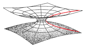
Figure 1: The setup: a string (shown in red) stretching between the two asymptotic boundaries of an eternal AdS black hole.

Before proceeding further, it will be convenient to recast the problem in terms of Kruskal coordinates, $t=\frac{1}{2r_{H}}\log(-\frac{u}{v})$ and $r=r_{H}(\frac{2}{1+uv}-1)$, and work in the gauge $(\tau,\sigma)=(u,v)$. The string in this case stretches between the two asymptotic boundaries of an eternal AdS black hole (see Fig. 1). For the static solution $X(u,v)=0$, we find that the induced metric is given by

$$ds_{{\scriptscriptstyle ws}}^{2}=-{4dudv\over(1+uv)^{2}},$$ (13)

i.e., an AdS₂ wormhole. The equations for the fluctuations over this embedding follow from the action

$$S_{\text{NG}}=-\frac{1}{\pi\alpha^{\prime}}\int dudv\sqrt{\frac{1-r_{H}^{2}(1-uv)^{2}\partial_{u}X\partial_{v}X}{(1+uv)^{4}}}.$$ (14)

3. Four-point OTOC. In order to compute the relevant OTOC, we will use the techniques and approximations developed in Shenker:2014cwa , adapted to the world sheet theory.

3.1 Overlapping states. We represent $D(\{t_{i}\})=\langle W(t_{1})V(t_{2})W(t_{3})V(t_{4})\rangle$ as the overlap of two states:

$$|\psi\rangle=W(t_{2})^{\dagger}V(t_{1})^{\dagger}|\Psi\rangle,\quad|\psi^{\prime}\rangle=V(t_{3})W(t_{4})|\Psi\rangle,$$ (15)

where $|\Psi\rangle$ is the two-sided purification: the thermofield double state. The $V$ and $W$ operators create two perturbations on the string. If the difference in times $t_{2}-t_{1}$ and $t_{4}-t_{3}$ are large, then the relative boosts between the wave packets are also large.

In Kruskal coordinates, the perturbation created by $W$ will have large $p^{v}$ and will be moving near the $u=0$ horizon. Similarly, the perturbation created by $V$ will have large $p^{u}$ and will be moving near the $v=0$ horizon. We represent the $W$ quantum in the Hilbert space on the $v=0$ horizon, and the $V$ quantum on the $u=0$ horizon. Then $|\psi^{\prime}\rangle$ is the “in” state

$$V(t_{3})W(t_{4})|\Psi\rangle=\int\psi_{3}(p_{3}^{u})\psi_{4}(p_{4}^{v})|p_{3}^{u}\,p_{4}^{v}\rangle_{\textrm{in}}.$$ (16)

Similarly, $|\psi\rangle$ is an “out” state given by

$$W(t_{2})V(t_{1})|\Psi\rangle=\int\psi_{1}(p_{1}^{u})\psi_{2}(p_{2}^{v})|p_{1}^{u}\,p_{2}^{v}\rangle_{\textrm{out}}.$$ (17)

The normalization of the states is given by

$$\langle p^{v}|q^{v}\rangle={4p^{v}\over\pi}\delta(p^{v}-q^{v}).$$ (18)

The wave functions can be expressed using the Fourier-transformed bulk-to-boundary propagators

$$\psi_{1}(p^{u})=\int dve^{2ip^{u}v}\langle\varphi_{V}(u,v)V(t_{1})^{\dagger}\rangle|_{u=0},$$ (19)

$$\psi_{2}(p^{v})=\int due^{2ip^{v}u}\langle\varphi_{W}(u,v)W(t_{2})^{\dagger}\rangle|_{v=0},$$ (20)

$$\psi_{3}(p^{u})=\int dve^{2ip^{u}v}\langle\varphi_{V}(u,v)V(t_{3})\rangle|_{u=0},$$ (21)

$$\psi_{4}(p^{v})=\int due^{2ip^{v}u}\langle\varphi_{W}(u,v)W(t_{4})\rangle|_{v=0},\vspace{-1cm}$$ (22)

where $\varphi_{V,W}$ are the world sheet fields dual to the operators $V$ and $W$. Finally, the four-point function is given by the overlap (see Fig. 2 for a pictorial representation)

$$D=\int d\{p_{i}\}\,\psi_{3}^{*}(p_{3}^{u})\,\psi_{4}^{*}(p_{4}^{v})\,\psi_{1}(p_{1}^{u})\,\psi_{2}(p_{2}^{v})\,{}_{\textrm{in}}\langle p_{3}^{u}\,p_{4}^{v}|p_{1}^{u}\,p_{2}^{v}\rangle_{\textrm{out}}$$ (23)

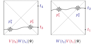
Figure 2: The four-point function (23) as an inner product of the two states (16) and (17). The solid lines represent spacelike slices of the string world sheet, while the wiggles correspond to operator insertions near the horizons.

We still need to compute the bracket in the integrand. In the center-of-mass frame, if the relative boost is large, then the momenta $p_{1}^{u},p_{2}^{v},p_{3}^{u},p_{4}^{v}$ are large and momentum conservation implies $p_{1}^{u}\approx p_{3}^{u}$, $p_{2}^{v}\approx p_{4}^{v}$. Within the two-particle Hilbert space, we can approximate $|p_{1}^{u}\,p_{2}^{v}\rangle_{\textrm{out}}\approx e^{i\delta(s)}|p_{1}^{u}\,p_{2}^{v}\rangle_{\textrm{in}}$, where $s=4p_{1}^{u}p_{2}^{v}$ is a Mandelstam variable.

3.2 Phase shift. Let us now compute $\delta(s)$. We define $R=v+u$, $T=v-u$ and rescale $X\to Xl_{s}/r_{H}$, where $l_{s}\equiv\sqrt{2\pi\alpha^{\prime}}$. At quadratic order, the action (14) reads

$$S_{0}={1\over 2}\int dTdR\left(\dot{X}^{2}-X^{\prime 2}\right).$$ (24)

We are interested in high-energy collisions near the horizons, so we considered the flat space approximation and set $uv=0$. In the center-of-mass frame, the solution for two equal perturbations moving in opposite directions is

$${X(T,R)}=F(T+R)+F(T-R),$$ (25)

where $F(\xi)$ is assumed to vanish outside a window around $\xi=0$. In this approximation, the two wave packets simply pass through each other. Let us now consider the subleading interacting term in the action:

$$S_{1}={l_{s}^{2}\over 8}\int dTdR\left(\dot{X}^{2}-X^{\prime 2}\right)^{2}.$$ (26)

Evaluating $S_{1}$ on the background of two wave packets will yield the phase shift. By plugging in (25), we get

$$S_{1}=l_{s}^{2}\left(\int d\xi F^{\prime}(\xi)^{2}\right)^{2}.$$ (27)

Since we have $\delta(s)=S_{1}$, all that is left to do is to express the action in terms of the Mandelstam variable of the collision. The target space current is given by

$$P^{a}_{\mu}=-\sqrt{-\gamma}\gamma^{ab}\eta_{\mu\nu}\partial_{b}X^{\nu}.$$ (28)

The string energy is then an integral over a spacelike slice on the world sheet

$$E[X]=-\int d\sigma P^{\tau}_{T}=\int d\sigma\sqrt{-\gamma}\gamma^{\tau b}\eta_{T\nu}\partial_{b}X^{\nu}.$$ (29)

This gives a divergent energy for the infinitely long string

$$E[F]\simeq\int dR\left[1+F^{\prime}(T-R)^{2}+F^{\prime}(T+R)^{2}+\cdots\right].$$ (30)

The expansion in terms of $|F^{\prime}|\ll 1$ is necessary, because we have neglected terms beyond $S_{1}$ in the expression for the phase shift. The energy of the wave packets is thus

$$\Delta E=E[F]-E[0]=2\int d\xi F^{\prime}(\xi)^{2},$$ (31)

and the Mandelstam variable is $s=(\Delta E)^{2}$. Comparing this formula with (27), we get

$$\delta(s)={sl_{s}^{2}\over 4}.$$ (32)

The phase shift can also be computed from light-cone quantization for a bosonic critical string as in Dubovsky:2012wk . It is easy to check that their method also reproduces our phase shift formula (32).

3.3 Integral over momenta. The bulk-to-boundary propagator for an operator with conformal dimension $\Delta$ is

$$\langle\phi(u,v){\cal O}(t^{\prime})\rangle=c_{\cal O}\left(\frac{1+uv}{ue^{t^{\prime}}-ve^{-t^{\prime}}+(1-uv)}\right)^{\Delta}\,,$$ (33)

where we have used Kruskal coordinates in the bulk and set $r_{H}=2\pi/\beta=1$ for simplicity. The temperature dependence can be restored by dimensional analysis whenever necessary. We evaluate these propagators at one of the horizons ($u,v=0$) and perform the Fourier transforms in (19)-(22):

$$\psi_{1}(p^{u},t_{1}) =-2\pi p^{u}\theta(p^{u})e^{2\,t_{1}^{*}+2ip^{u}e^{t_{1}^{*}}},$$ (34)

$$\psi_{2}(p^{v},t_{2}) =i\pi p^{v}\theta(p^{v})e^{-\,t_{2}^{*}-2ip^{v}e^{-t_{2}^{*}}},$$ (35)

$$\psi_{3}(p^{u},t_{3}) =-2\pi p^{u}\theta(p^{u})e^{2\,t_{3}+2ip^{u}e^{t_{3}}},$$ (36)

$$\psi_{4}(p^{v},t_{4}) =i\pi p^{v}\theta(p^{v})e^{-\,t_{4}-2ip^{v}e^{-t_{4}}},$$ (37)

where the complex conjugate in $t_{1}$ and $t_{2}$ appears because we are considering Hermitian conjugates for the first and the second propagators in $|\psi\rangle$. Since $W(t)=x(t)$ and $V(t)=\dot{x}(t)$, we have already set $\Delta_{W}=1$ and $\Delta_{V}=2$. With (34)-(37) and $\delta=p^{u}p^{v}\,l_{s}^{2}$, we are ready to perform the overlap integration (23). By changing the variables $p^{u}=-\frac{p}{2i\left(-e^{t_{1}}+e^{t_{3}}\right)}$ and $p^{v}=\frac{q}{2i\left(-e^{t_{2}}+e^{t_{4}}\right)}$ and fixing the end points as $t_{1}=i\epsilon_{1},\,t_{2}=t+i\epsilon_{2},\,t_{3}=i\epsilon_{3},\,t_{4}=t+i\epsilon_{4}$, we find

$$\langle V(i\epsilon_{1})W(t+i\epsilon_{2})V(i\epsilon_{3})W(t+i\epsilon_{4})\rangle=$$

$$\qquad\qquad\qquad\qquad C\int_{0}^{\infty}dpdq\,p^{3}q\,e^{-p-q}e^{il_{s}^{2}e^{t}pq/4\epsilon_{13}\epsilon_{24}^{*}},$$ (38)

$$\langle V(i\epsilon_{1})V(i\epsilon_{3})\rangle\,\langle W(t+i\epsilon_{2})W(t+i\epsilon_{4})\rangle=$$

$$\qquad\qquad\qquad\qquad C\int_{0}^{\infty}dpdq\,p^{3}q\,e^{-p-q},$$ (39)

where we have defined the constants

$$C\equiv c_{V}^{2}c_{W}^{2}\frac{\pi^{4}}{1024}\csc^{4}\left(\frac{\epsilon_{1}-\epsilon_{3}}{2}\right)\csc^{2}\left(\frac{\epsilon_{2}-\epsilon_{4}}{2}\right),$$ (40)

$$\epsilon_{ij}\equiv i(e^{i\epsilon_{i}}-e^{i\epsilon_{j}}).$$ (41)

The integrals above can be computed exactly in terms of the exponential integral, $Ei(z)=-\int^{\infty}_{-z}e^{-t}dt$. However, the results can be trusted only up to $\mathcal{O}(l_{s}^{2})$, since we truncated the action at this order. Performing this approximation, the normalized four-point function reads

$$\frac{\langle V(i\epsilon_{1})W(t+i\epsilon_{2})V(i\epsilon_{3})W(t+i\epsilon_{4})\rangle}{\langle V(i\epsilon_{1})V(i\epsilon_{3})\rangle\,\langle W(t+i\epsilon_{2})W(t+i\epsilon_{4})\rangle}\simeq 1+\frac{2il_{s}^{2}e^{t}}{\epsilon_{13}\epsilon_{24}^{*}}.$$ (42)

3.4 Scrambling and Lyapunov exponent. Although we denoted the imaginary time parameters as $\epsilon_{i}$, they do not necessarily have to be small. For instance, if we subtract $\beta/2$ from $\epsilon_{1}$ and add the same to $\epsilon_{4}$, we can obtain two-sided correlators from the above one-sided expectation value. A canonical choice made in Maldacena:2015waa consists in setting $\epsilon_{1}=\beta/2=\pi$, $\epsilon_{2}=-\beta/4=-\pi/2$, $\epsilon_{3}=0$, $\epsilon_{4}=\beta/4=\pi/2$. This corresponds to the insertion of the $V$ and $W$ operators at equal spacing around the thermal circle. With this choice, one gets $\epsilon_{13}=-2i$ and $\epsilon_{24}=2$. Finally, by restoring the temperature dependence, we find that the four-point function (2) is given by

$$f(t)=1-\frac{\pi}{\sqrt{\lambda}}e^{2\pi t/\beta}.$$ (43)

The above equation must be contrasted with the result for correlator in the pure gravity sector (3). From (43), we can read off the Lyapunov exponent

$$\lambda_{L}=\frac{2\pi}{\beta},$$ (44)

which saturates the bound (5), and the scrambling time

$$t_{*}\sim\beta\log\sqrt{\lambda}.$$ (45)

Thus, even though the world sheet theory is not gravitational, it is maximally chaotic and exhibits the fast scrambling property of black holes. In addition, there is also a parametrically large hierarchy between scrambling and dissipation determined, in this case, by the small parameter $\alpha^{\prime}\sim 1/\sqrt{\lambda}$ instead of the standard $G_{N}\sim 1/N^{2}$. The fact that $t_{*}$ scales the way it does can be easily understood, since $\sqrt{\lambda}$ is proportional to the excess of entropy due to the probe string (11), and these are precisely the degrees of freedom that are being scrambled.

4. Complexity. Black holes are known to excel at another information theoretic task, namely, the processing of information. The rate of quantum information processing is measured by computational complexity $\mathcal{C}$. Complexity counts the minimal number of gates needed to build a quantum circuit which prepares the state from a particular reference state. It grows linearly at late times and obeys the bound $d\mathcal{C}/dt\leq 2E/\pi\hbar$ Lloyd . It is then interesting to ask about complexity in our present setup.

In AdS/CFT, there are two proposals to compute complexity, the Complexity$=$Volume CV and the Complexity$=$Action CA conjectures, both satisfying the bound. In the former, the complexity is proportional to the spatial volume of the Einstein-Rosen bridge $V$:

$$\mathcal{C}\sim\frac{V}{G_{N}\ell},$$ (46)

where $\ell$ is some length scale. This quantity does indeed grow linearly over time at late times. In order to compute the correction to $\mathcal{C}$ due to the probe string, one would need to consider the backreaction of the string on the bulk geometry and compute the new volume $V$. Here we proceed differently. We define the dimensionless quantity

$$\mathcal{C}_{{\scriptscriptstyle ws}}=\frac{\tilde{\ell}\hskip 1.00006ptV_{{\scriptscriptstyle ws}}}{\alpha^{\prime}},$$ (47)

as a “world sheet complexity”, where $\tilde{\ell}$ is a time scale and $V_{{\scriptscriptstyle ws}}$ is the length of the world sheet wormhole. A brief computation yields at late times

$$\frac{dV_{{\scriptscriptstyle ws}}}{dt}=\frac{2\pi}{\beta}\quad\rightarrow\quad\frac{d\mathcal{C}_{{\scriptscriptstyle ws}}}{dt}=\text{const}.$$ (48)

It would be interesting to ask about its significance in the CFT language. The second proposal for complexity gets rid of the arbitrary length scale $\ell$ and states that

$$\mathcal{C}\sim\frac{\mathcal{S}_{\text{WDW}}}{\pi\hbar},$$ (49)

where $\mathcal{S}_{\text{WDW}}$ is the bulk action evaluated on the Wheeler-DeWitt patch. The correction of $\mathcal{C}$ due to the probe string in this case is simpler: it is given by the NG action evaluated on the Wheeler-DeWitt patch flavorcomplexity . Notice that if we were to define a world sheet complexity using the world sheet geometry, the result would be equivalent to (49). However, at least in $d=3$ we find that there is an ambiguity on defining the Wheeler-DeWitt patch, because the maximally extended world sheet geometry gets past the $uv=1$ edges (cf. Fig. 5 in Hubeny:2014kma ). We hope to come back to this point in the future.

5. Discussion. We have presented the first example of a nongravitational system that is maximally chaotic, i.e., that saturates the universal bound on the Lyapunov exponent (5). The other two known examples that saturate the bound AdS black holes in Einstein gravity Maldacena:2015waa and the SYK model SYK , which contains an AdS₂ dilaton gravity sector Maldacena:2016hyu . Even though the world sheet theory does not contain gravitational degrees of freedom, it is worth recalling that the world sheet theory of strings shares some interesting similarities with theories of quantum gravity, including the absence of local off-shell observables, a minimal length, a maximum achievable (Hagedorn) temperature, as well as (integrable relatives of) black holes Dubovsky:2012wk .

In summary, the maximal chaotic exponent for the string follows from the following two points: $i)$ the induced world sheet metric has a horizon; therefore, by Rindler kinematics, the relation between world sheet scattering energy and time is $s\sim e^{2\pi t/\beta}$. And $ii)$ the eikonal phase is $\delta\sim\alpha^{\prime}s^{p}$ with $p=1$. This result is quite nontrivial. In ordinary QFT, a spin $J$ field exchanged in the Mandelstam $t$ channel gives $p=J-1$. Causality and unitarity further constrain the value of the exponent to be $p\leq 1$, since $e^{i\delta(s)}$ must be analytic in the upper half of the complex $s$ plane and $|e^{i\delta(s)}|\leq 1$ Camanho:2014apa . The NG theory has infinitely many higher derivative nonrenormalizable terms that appear nonlinearly in the action. As explained in Zamolodchikov:1991vx , the requirements of unitarity, crossing symmetry, and analyticity restrict the phase shift to take the form

$$e^{i2\delta{(s)}}=\prod_{j}\frac{\mu_{j}+s}{\mu_{j}-s}e^{iP(s)}\,,$$ (50)

where $P(s)$ is an odd polynomial in $s$ and $\mu_{j}$ are located in the lower half of the complex plane and either lie on the imaginary axis or come in pairs symmetric with respect to it. What is surprising is that the $\mu_{j}$ and $P(s)$ for the NG theory conspire to give the required phase shift mimicking a single graviton exchange (see also Dubovsky:2012wk ).

Finally, let us comment on the extension of the chaos bound conjectured in Maldacena:2015waa to our setup. The proof of the maximal Lyapunov exponent relies on two points. The first one is a result bounding the derivative of any function, which was shown to hold in general. The second one is the assumption that the error $\varepsilon$ of the late-time factorization of the OTOC is small. A quick calculation shows that in our setup $\varepsilon\sim 1/\sqrt{\lambda}$, which holds true as long as $\lambda$ is large. This, together with the fact that $\delta(s)\sim s$ seems to hold beyond leading order Dubovsky:2012wk , suggests that perturbative higher-order $\alpha^{\prime}$ corrections should respect the bound, although it would be interesting to see an explicit calculation. Furthermore, at weak ’t Hooft coupling, the strength of scattering in the gauge theory is of the order of $\lambda$, so one would expect $\lambda_{L}\sim\lambda/\beta$, parametrically smaller than the strong coupling result.

There are a few directions that may be worth exploring in the future. Two interesting generalizations to consider are $i)$ a higher-dimensional target space and $ii)$ higher-dimensional probes in the bulk such as $Dp$-branes. From the latter, one could also compute the associated butterfly velocities and compare with the charge diffusion results Diffusion . One could also repeat the computations of the OTOC presented here in more complex shockwave geometries, i.e., segmented strings in AdS space Segmented . Finally, it would be interesting to understand whether the chaotic behavior observed here can emerge in other field theories in a black hole background or whether there are specific features of the string action that make it chaotic.

Note added: Recently, we became aware of Murata:2017rbp whose results overlap with ours.

Acknowledgements. We are grateful to M. Chernicoff, V. Hubeny, and D. Stanford for discussions and useful correspondence. This work is supported by the Netherlands Organisation for Scientific Research (NWO) and the Delta-Institute for Theoretical Physics ($\Delta$-ITP).

References

- (1) J. Maldacena, S. H. Shenker and D. Stanford, JHEP 1608, 106 (2016).
- (2) S. H. Shenker and D. Stanford, JHEP 1403, 067 (2014).
- (3) S. H. Shenker and D. Stanford, JHEP 1505, 132 (2015).
- (4) S. H. Shenker and D. Stanford, JHEP 1412, 046 (2014); S. Leichenauer, Phys. Rev. D 90, no. 4, 046009 (2014); D. A. Roberts, D. Stanford and L. Susskind, JHEP 1503, 051 (2015); D. A. Roberts and B. Swingle, Phys. Rev. Lett. 117, no. 9, 091602 (2016); N. Sircar, J. Sonnenschein and W. Tangarife, JHEP 1605, 091 (2016); K. Jensen, Phys. Rev. Lett. 117, no. 11, 111601 (2016); R. G. Cai, X. X. Zeng and H. Q. Zhang, JHEP 1707, 082 (2017); M. M. Qaemmaqami, Phys. Rev. D 96, no. 10, 106012 (2017); V. Jahnke, arXiv:1708.07243 [hep-th].
- (5) D. A. Roberts and D. Stanford, Phys. Rev. Lett. 115, no. 13, 131603 (2015); A. L. Fitzpatrick and J. Kaplan, JHEP 1605, 070 (2016).
- (6) Y. Sekino and L. Susskind, JHEP 0810, 065 (2008); N. Lashkari, D. Stanford, M. Hastings, T. Osborne and P. Hayden, JHEP 1304, 022 (2013).
- (7) B. Michel, J. Polchinski, V. Rosenhaus and S. J. Suh, JHEP 1605, 048 (2016); P. Caputa, T. Numasawa and A. Veliz-Osorio, PTEP 2016, no. 11, 113B06 (2016); E. Perlmutter, JHEP 1610, 069 (2016); G. Turiaci and H. Verlinde, JHEP 1612, 110 (2016); P. Caputa, Y. Kusuki, T. Takayanagi and K. Watanabe, Phys. Rev. D 96, no. 4, 046020 (2017); A. Belin, arXiv:1705.08451 [hep-th].
- (8) J. de Boer, V. E. Hubeny, M. Rangamani and M. Shigemori, JHEP 0907, 094 (2009); D. T. Son and D. Teaney, JHEP 0907, 021 (2009); G. C. Giecold, E. Iancu and A. H. Mueller, JHEP 0907, 033 (2009); M. Chernicoff, J. A. Garcia, A. Guijosa and J. F. Pedraza, J. Phys. G 39, 054002 (2012); W. Fischler, J. F. Pedraza and W. Tangarife Garcia, JHEP 1212, 002 (2012); A. N. Atmaja, J. de Boer and M. Shigemori, Nucl. Phys. B 880, 23 (2014); W. Fischler, P. H. Nguyen, J. F. Pedraza and W. Tangarife, JHEP 1408, 028 (2014);
- (9) B. W. Xiao, Phys. Lett. B 665, 173 (2008); E. Caceres, M. Chernicoff, A. Guijosa and J. F. Pedraza, JHEP 1006, 078 (2010); J. A. Garcia, A. Guijosa and E. J. Pulido, JHEP 1301, 096 (2013).
- (10) K. Jensen and A. Karch, Phys. Rev. Lett. 111, no. 21, 211602 (2013); J. Sonner, Phys. Rev. Lett. 111, no. 21, 211603 (2013); M. Chernicoff, A. Guijosa and J. F. Pedraza, JHEP 1310, 211 (2013).
- (11) J. Maldacena and L. Susskind, Fortsch. Phys. 61, 781 (2013).
- (12) M. Spradlin and A. Strominger, JHEP 9911, 021 (1999).
- (13) S. Sachdev and J. Ye, Phys. Rev. Lett. 70, 3339 (1993); A. Kitaev, http://online.kitp.ucsb.edu/online/entangled15/kitaev/,http://online.kitp.ucsb.edu/online/entangled15/kitaev2/. Talks at KITP, April 7, 2015 and May 27, 2015.
- (14) J. Maldacena and D. Stanford, Phys. Rev. D 94, no. 10, 106002 (2016).
- (15) K. Jensen and A. O’Bannon, Phys. Rev. D 88, no. 10, 106006 (2013).
- (16) A. I. Larkin and Y. N. Ovchinnikov, JETP 28, 6 (1969), 1200-1205.
- (17) S. Giombi, R. Roiban and A. A. Tseytlin, Nucl. Phys. B 922, 499 (2017).
- (18) S. Dubovsky, R. Flauger and V. Gorbenko, JHEP 1209, 133 (2012).
- (19) S. Lloyd, Nature 406 (2000), no. 6799 1047–1054.
- (20) L. Susskind, [Fortsch. Phys. 64, 24 (2016)]; D. Stanford and L. Susskind, Phys. Rev. D 90, no. 12, 126007 (2014).
- (21) A. R. Brown, D. A. Roberts, L. Susskind, B. Swingle and Y. Zhao, Phys. Rev. Lett. 116, no. 19, 191301 (2016); Phys. Rev. D 93, no. 8, 086006 (2016)
- (22) F. J. G. Abad, M. Kulaxizi and A. Parnachev, arXiv:1705.08424 [hep-th]; K. Nagasaki, arXiv:1707.08376 [hep-th].
- (23) V. E. Hubeny and G. W. Semenoff, JHEP 1510, 071 (2015).
- (24) X. O. Camanho, J. D. Edelstein, J. Maldacena and A. Zhiboedov, JHEP 1602, 020 (2016).
- (25) A. B. Zamolodchikov, Nucl. Phys. B 358, 524 (1991).
- (26) M. Blake, Phys. Rev. Lett. 117, no. 9, 091601 (2016); M. Blake, Phys. Rev. D 94, no. 8, 086014 (2016); R. A. Davison, W. Fu, A. Georges, Y. Gu, K. Jensen and S. Sachdev, Phys. Rev. B 95, no. 15, 155131 (2017); D. Giataganas, U. Gursoy and J. F. Pedraza, arXiv:1708.05691 [hep-th].
- (27) D. Vegh, arXiv:1508.06637 [hep-th]; N. Callebaut, S. S. Gubser, A. Samberg and C. Toldo, JHEP 1511, 110 (2015).
- (28) K. Murata, arXiv:1708.09493 [hep-th].