Symmetric Treatment Decomposition Of Spillover Effects

Abstract

Classical causal inference assumes treatments meant for a given unit do not have an effect on other units. This assumption is violated in interference problems, where new types of spillover causal effects arise, and causal inference becomes much more difficult. In addition, interference introduces a unique complication where variables may transmit treatment influences to each other, which is a relationship that has some features of a causal one, but is symmetric. In settings where a natural causal ordering on variables is not available, addressing this complication using statistical inference methods based on Directed Acyclic Graphs (DAGs) leads to conceptual difficulties. In this paper, we develop a new approach to decomposing the spillover effect into unit-specific components that extends the DAG based treatment decomposition approach to mediation of Robins and Richardson. We give conditions for these components of the spillover effect to be identified in a natural type of causal model that permits stable symmetric relations among outcomes induced by a process in equilibrium. We discuss statistical inference for identified components of the spillover effect, including a maximum likelihood estimator, and a doubly robust estimator for the special case of two interacting outcomes. We verify consistency and robustness of our estimators via a simulation study, and illustrate our method by assessing the causal effect of education attainment on depressive symptoms using the data on households from the Wisconsin Longitudinal Study.

Keywords: chain graphs; graphical models; interference; mediation analysis; semi-parametric inference

1 Introduction

A standard assumption in causal inference is absence of unit interference, which asserts that giving treatment to a particular unit only affects the response of that unit. While a sensible assumption in many statistical application, there are settings where this assumption is not reasonable. A classic example from infectious disease epidemiology is herd immunity: vaccinating a subset of a population may grant immunity to the unvaccinated members of the population. Another example is medical triage, where shortages of effective treatments may induce dependence between the clinical outcome of one patient (say one assigned low priority by the triage procedure), and the treatment assigned to another patient.

The presence of interference introduces a number of conceptual difficulties. First, unlike classical causal inference, variables associated with experimental units can no longer be viewed as independent realizations of some underlying distribution. Second, new types of causal effects called spillover effects arise, which quantify the degree to which treatments for one unit affect the outcome of another unit. Like total causal effects from classical causal inference, it may be of scientific interest to decompose spillover effects into direct and indirect components, and more generally into unit-specific components.

In the context of infectious disease epidemiology, the direct and indirect components of the spillover effect are called the infectiousness effect, and the contagion effect, respectively (VanderWeele et al., 2012). In the context of data-driven online marketing, decomposing the effect of an advertisement on purchasing or voting behavior of a set of people forming a social network into a set of unit-specific components may also be of substantive interest. In particular, the magnitude of these unit-specific effects can help quantify which sorts of people drive the overall response to an advertisement in a network.

Prior work has used ideas from the mediation analysis literature to obtain decompositions of spillover effects (VanderWeele et al., 2012). Such an approach is not appropriate in interference settings where unit outcomes do not form a natural causal ordering. We propose an alternative approach to interference that places dependent outcomes forming a network “on the same footing.” Our model can be viewed as either a symmetric generalization of classical mediation analysis (Robins and Greenland, 1992; Pearl, 2001) to interference settings without a total causal order on variables, or as a generalization of the treatment decomposition formalism for mediation analysis advocated in Robins and Richardson (2010) to models of interference that capture equilibria of causal feedback processes given by structural equations (Lauritzen and Richardson, 2002).

1.1 A Motivating Example And Outline Of Contributions

We begin with an example described in VanderWeele et al. (2012), and motivated by a study described in Trollfors et al. (1998). In this hypothetical example, one-year-old children at a day care center are randomized to receive a vaccine (denoted by $A=a$) or placebo (denoted by $A=a^{\prime}$) against a particular pathogen serotype prevalent in children attending day care. A number of questions may be of interest in such a study. A question of primary interest may be the causal effect of vaccination on pathogen colonization status in the child (denoted by $Y^{1}$). A secondary question would be a similar causal effect: that of vaccination on the pathogen colonization status in the care provider (e.g. mother) of the child, denoted by $Y^{2}$. Note that since the child and care provider live in the same household, the potential for disease spread implies the outcomes $Y^{1},Y^{2}$ should be modelled as associated random variables. In other words, variable pairs pertaining to children and care providers should not be viewed as independent realizations of an underlying distribution, but as forming a dependent dyad data structure.

In addition to variables explicitly mentioned, that is the treatment $A$, and the outcomes of the child/care provider dyad $Y^{1},Y^{2}$, the study may also record a set of relevant baseline covariates $\vec{C}$, for both the child and the care provider. These covariates may be used to assign the vaccine or placebo treatment (corresponding to values of $A$) via a distribution $p(A\mid\vec{C})$ corresponding to a known design rule, or an assignment probability that must be learned from data.

Causal effects are often conceptualized via potential outcome random variables (Neyman, 1923; Rubin, 1976). For example, the potential outcome $Y^{1}(a)$ denotes colonization status in the child had, possibly contrary to fact, the child had been vaccinated. Causal effects are generally defined using potential outcomes as contrasts on the mean scale. For instance, the average causal effect of vaccination on colonization status of the child would be defined as: $\mathop{\mathbb{E}}[Y^{1}(a)]-\mathop{\mathbb{E}}[Y^{1}(a^{\prime})]$, while the similar average spillover effect of vaccination of the child on colonization status of the care provider would be defined as $\mathop{\mathbb{E}}[Y^{2}(a)]-\mathop{\mathbb{E}}[Y^{2}(a^{\prime})]$.

Decomposition of an established spillover effect into components is of interest in cases where these components can be isolated and have a substantive interpretation. In our example, the presence of an indirect component of the spillover effect, known as the contagion effect, indicates that vaccinating units directly lessens the chance of infection of those units, and thus the chance of those units passing the infection on. Similarly, the presence of a direct component of the spillover effect, known as the infectiousness effect, indicates that vaccinating units may modify the chance of infection in some other way, perhaps by suppressing more virulent strains from propagating.

There are two complementary views of causal relationships underlying variables in the example we outlined, which influence how the spillover effect and its unit-specific components are defined, identified and estimated. The distinction between the two views concerns the causal relationships of $A$ and $\vec{C}$ and outcomes of the child and the caregiver: $Y^{1}$ and $Y^{2}$. The modeling choice made in VanderWeele et al. (2012) proceeds by assuming that a child’s caregiver is only likely to get infected with the pathogen through their child, who in turn would have obtained the infection from daycare. This assumption, which is sensible if the pathogen is a childhood disease such as pertussis, imposes a natural causal ordering where variables $A$ and $\vec{C}$ cause both $Y^{1}$ and $Y^{2}$, and $Y^{1}$ causes $Y^{2}$. A popular representation of causal models with variables that follow a known ordering is via directed acyclic graphs (DAGs). Such a graph for our model is shown in Fig. 1 (a), with vertices representing random variables in the problem, and directed edges between vertices meaning, in the sense to be made precise below, “direct causation.” In this view, spillover effects can be defined as standard causal effects, and direct and indirect components of the spillover effects can be defined using tools of mediation analysis, as described in VanderWeele et al. (2012), and below.

However, this approach is less sensible for pathogens that could be caught by either the child or the caregiver (such as COVID-19), since there is no unambiguous causal order on the outcomes $Y^{1},Y^{2}$ in such cases. A popular approach for causal models of this sort has been developed in the partial interference literature (Hudgens and Halloran, 2008; Tchetgen Tchetgen and VanderWeele, 2012). In the partial interference view, outcome variables $Y^{1},Y^{2}$ (and their corresponding counterfactuals $Y^{1}(a),Y^{2}(a)$) are defined jointly as a “block”, with no clear causal ordering on variables within the block.

In this paper, we show that the spillover effect, and its direct, indirect, and unit-specific components can be formally represented as potential outcomes in causal models that do not require a total causal ordering on variables, and allow jointly defined counterfactuals of the above sort. In particular, we consider causal models allowing variable relationships that are symmetric, stable (meaning that they remain invariant under interventions), and generated by a causal feedback process (Lauritzen and Richardson, 2002). A graphical representation of such a model is shown in Fig. 1 (c), where directed edges have the same meaning as in a causal DAG, while the undirected edge between $Y^{1}$ and $Y^{2}$ represents a particular type of symmetric dependence between outcomes. See Lauritzen (1996) and Cox and Wermuth (1993) for additional discussion of graphical models with symmetric relationships between variables.

We further show how these effects may be identified via a key assumption that generalizes assumptions made in mediation analysis. In the dyadic context, we call the resulting identifying functional for direct and indirect components of the spillover effect the symmetric mediation formula, due to the fact that it can be viewed as an appropriate generalization of the mediation formula in directed acyclic graph models (Pearl, 2011). In general network contexts, unit-specific effects we define may be viewed as natural analogues of general edge specific interventions arising in mediation analysis in directed acyclic graph (DAG) models (Shpitser and Tchetgen Tchetgen, 2016).

In addition, we demonstrate that identifying assumptions in our models impose restrictions on the observed data law, which leads to falsifiability (but not testability) of our models, a desirable feature not present in the classical mediation setting. Finally, we consider estimation of functionals identifying components of spillover effects as an inference problem in statistical chain graph models. We derive maximum likelihood estimators that is straightforward to implement. In settings when dyadic outcomes are labeled, e.g parent and child or husband and wife, we describe a semi-parametric doubly robust estimator for the symmetric mediation formula.

We then apply our derived estimators to both a real-world example and simulated data. We use data taken from the Wisconsin Longitudinal Study, a longitudinal cohort of Wisconsin high school graduates and their spouses, to decompose the effect of educational attainment on depressive symptoms, taking into account covariates and likely interference between husband and wife pairs. To illustrate the behavior of our doubly robust estimator, we designed a simulation study for spillover effect components in both randomized treatment and non-randomized treatment settings.

Figure 1: (a) A directed acyclic graph (DAG) representing a common causal model for mediation analysis. (b) An elaboration of the DAG in (a) considered in (Robins and Richardson, 2010) which represents a counterfactual used to define direct and indirect effects as a response to two edge-specific interventions. counterfactual as a response to two pathway-specific interventions. (c) A causal model representing a partial interference causal inference setting with a dyad outcome. (d) An elaboration of the graph in (c) which represents an interference counterfactual as a response to two dyad outcome specific interventions.

2 Notation and Preliminaries

Here we describe the necessary preliminaries: causal models, mediation analysis, and extensions of causal models that permit reasoning about interference.

2.1 Classical Causal Inference

Causal inference aims to use realizations of the observed data distribution $p(\vec{V})$ to make inferences about parameters defined using potential outcome random variables. In our running example, a potential outcome $Y^{1}(a)$ denotes what would happen to the outcome $Y^{1}$ (the child’s colonization status) had the treatment $A$ been set, possibly contrary to fact, to $a$ (vaccination).

Potential outcomes have been used to quantify causal effect relationships between the treatment $A$ and the outcome $Y$ by the parameter known as the average causal effect (ACE): $\beta\equiv\mathop{\mathbb{E}}[Y(a)]-\mathop{\mathbb{E}}[Y(a^{\prime})]$, representing the average outcomes in two arms of a hypothetical randomized controlled trial with the two arms given treatment values $a$ and $a^{\prime}$.

The difficulty with the ACE parameter is that it is a function of responses that occur contrary to fact. The fundamental problem of causal inference is that we only observe the response actually assigned. A link between counterfactual contrasts such as the ACE, and observed data is typically made by means of the consistency assumption, and some version of the ignorability assumption.

Consistency provides a link between observed and counterfactual outcomes by asserting that the random variable representing the outcome $Y$ is equal to the random variable representing the outcome $Y(A)$ where $A$ is set to whatever value it actually obtained. The popular version of ignorability states that the treatment assignment probability $A$ is independent of the potential outcomes $Y(a),Y(a^{\prime})$ conditional on a set of baseline covariates $\vec{C}$. Under these assumptions, as well as the assumption of positivity, where $p(A\mid\vec{C})>0$, we have

$$\mathop{\mathbb{E}}[Y(a)]-\mathop{\mathbb{E}}[Y(a^{\prime})] =\mathop{\mathbb{E}}[\mathop{\mathbb{E}}[Y(a)\,|\,\vec{C}]-\mathop{\mathbb{E}}[Y(a^{\prime})\,|\,\vec{C}]]$$

$$=\mathop{\mathbb{E}}[\mathop{\mathbb{E}}[Y(a)\,|\,a,\vec{C}]-\mathop{\mathbb{E}}[Y(a^{\prime})\,|\,a^{\prime},\vec{C}]]$$

$$=\mathop{\mathbb{E}}[\mathop{\mathbb{E}}[Y\,|\,a,\vec{C}]-\mathop{\mathbb{E}}[Y\,|\,a^{\prime},\vec{C}]],$$

where the first equality is by the tower law, the second by conditional ignorability and positivity, and the last by consistency.

If the above assumption of conditional ignorability does not hold by design, more complex assumptions are used to obtain identification of counterfactual contrasts in terms of observed data. These assumptions are often phrased in terms of directed acyclic graphs (DAGs), where vertices represent variables of interest, and directed edges represent direct causal relationships.

The DAG representing the causal model for our vaccination study example is shown in Fig. 1 (a). Formally, such a model corresponds to a set of independence assumptions on potential outcome random variables. It is common to assume, explicitly or implicitly, the non-parametric structural equation model with independent errors (NPSEM-IE) of Pearl (2009). This model associates a set of variables and a set of vertices ${\vec{V}}=\{V_{1},\ldots,V_{k}\}$ in a DAG, and for each variable $V_{i}\in{\vec{V}}$ assumes a noise variable $\epsilon_{V_{i}}$, and an arbitrary, invariant causal mechanism $f_{V_{i}}:{\mathfrak{X}}_{\operatorname{pa}_{\cal G}(V_{i})\cup\{\epsilon_{V_{i}}\}}\mapsto{\mathfrak{X}}_{V_{i}}$ mapping values of parents of $V_{i}$ in the graph ($\operatorname{pa}_{\cal G}(V_{i})$) and $\epsilon_{V_{i}}$ to values of $V_{i}$. It is assumed $f_{V_{i}}$ determines the value of $V_{i}$ regardless of how the values of $\operatorname{pa}_{\cal G}(V_{i})$ were assigned. Moreover, it is assumed the noise variables are mutually independent: $p(\epsilon_{V_{1}},\ldots\epsilon_{V_{k}})=\prod_{i=1}^{k}p(\epsilon_{i})$. The arbitrary nature of $f_{V_{i}}$ justifies the word “non-parametric,” and this property justifies the phrase “independent errors” in the name of the model. Interventions are represented by replacing certain mechanisms by constant values.

The four vertex example in Fig. 1 (a) is represented by four functions $f_{\vec{C}}:{\mathfrak{X}}_{\epsilon_{\vec{C}}}\mapsto{\mathfrak{X}}_{\vec{C}}$, $f_{A}:{\mathfrak{X}}_{\vec{C},\epsilon_{A}}\mapsto{\mathfrak{X}}_{A}$, $f_{Y^{1}}:{\mathfrak{X}}_{\{\vec{C},A,\epsilon_{Y^{1}}\}}\mapsto{\mathfrak{X}}_{Y^{1}}$, and $f_{Y^{2}}:{\mathfrak{X}}_{\{\vec{C},A,M,\epsilon_{Y}\}}\mapsto{\mathfrak{X}}_{Y^{2}}$. The intervention that sets $A$ to $a$ is conceptualized by replacing the structural equation $f_{A}$ by a constant function $\tilde{f}_{A}$ that outputs the value $a$, regardless of the input values of $\vec{C}$ and $\epsilon_{A}$.

An alternative definition of the NPSEM-IE model for a DAG ${\cal G}$ with a vertex set ${\vec{V}}$, given in Richardson and Robins (2013), uses one step ahead counterfactuals of the form $V(\vec{a}_{V})$, for any $\vec{a}_{V}\in{\mathfrak{X}}_{\operatorname{pa}_{\cal G}(V)}$, to define all other variable, factual or counterfactual, using recursive substitution. Specifically, for any $\vec{A}\subseteq{\vec{V}}$, and any $\vec{a}\in{\mathfrak{X}}_{\vec{A}}$, we have for every $V\in{\vec{V}}$

$$V(\vec{a})\equiv V(\vec{a}_{\operatorname{pa}_{\cal G}(V)},\{W(\vec{a}):W\in\operatorname{pa}_{\cal G}(V)\setminus\vec{A}\})$$ (1)

Given an arbitrary $V(\vec{a})$, recursive substitution (1) implies $V(\vec{a})$ is only a function of values $\vec{a}^{*}$ in $\vec{a}$ corresponding to elements in $\vec{A}$ with a directed path to $V$ not through other elements in $\vec{A}$. Such constraints are sometimes termed exclusion restrictions. As an example, $Y^{1}(a,y^{2})$ in the DAG ${\cal G}$ in Fig 1 (a) is only a function of $a$ and not of $y^{2}$.

Other restrictions defining the NPSEM-IE model are entailed by a set of assumptions on one-step-ahead counterfactuals, as a kind of causal version of the local Markov property. These assumptions state that

$$\text{``sets of variables in the set}\left\{\{V(\vec{a}_{V})\mid\vec{a}_{V}\in{\mathfrak{X}}_{\operatorname{pa}_{\cal G}(V)}\}\middle|V\in{\vec{V}}\right\}\text{are mutually independent.''}$$ (2)

This assumption is equivalent to the independent errors assumption above. In Fig. 1 (a), this assumption states that the following sets of variables are mutually independent:

$$\{\vec{C}\}\!\perp\!\!\!\perp\!\{A(\vec{c})\!:\!\vec{c}\in{\mathfrak{X}}_{\vec{C}}\}\!\perp\!\!\!\perp\!\{Y^{1}(a,\vec{c})\!:\!a\in{\mathfrak{X}}_{A},\vec{c}\in{\mathfrak{X}}_{\vec{C}}\}\!\perp\!\!\!\perp\!\{Y^{2}(y^{1},a,\vec{c})\!:\!y^{1}\in{\mathfrak{X}}_{Y^{1}},a\in{\mathfrak{X}}_{A},\vec{c}\in{\mathfrak{X}}_{\vec{C}}\}.$$ (3)

A weaker model known as the finest fully randomized causally interpretable structured tree graph (FFRCISTG) model for a DAG ${\cal G}$, described in Robins (1986), entails a weaker set of assumptions than (2):

$$\text{``variables in the set}\left\{V(\vec{v}_{V})\middle|V\in\vec{V}\right\}\text{are mutually independent for any }\vec{v}\in{\mathfrak{X}}_{\vec{V}}\text{.''}$$ (4)

In Fig. 1 (a), this assumption states that the following sets of variables are mutually independent for any $\vec{v}\in{\mathfrak{X}}_{\vec{C}\cup\{A,Y^{1},Y^{2}\}}$:

$$\{\vec{C},A(\vec{v}_{\vec{C}}),Y^{1}(\vec{v}_{\vec{C}\cup\{A\}}),Y^{2}(\vec{v}_{\vec{C}\cup\{A,Y^{1}\}})\}.$$ (5)

Note that (4) is a subset of assumptions in (2), meaning that the FFRCISTG model is a submodel of the NPSEM-IE.

It has been shown in Richardson and Robins (2013) that (1) and (4) entail that the observed data law obeys the standard Markov factorization with respect to the DAG ${\cal G}$:

$$p({\vec{V}})=\prod_{V\in{\vec{V}}}p(V(\operatorname{pa}_{\cal G}(V)))=\prod_{V\in{\vec{V}}}p(V\mid\operatorname{pa}_{\cal G}(V)),$$ (6)

and every interventional distribution of the form $p(\{W(\vec{a}):W\in\vec{V}\setminus\vec{A}\})$ is identified by a truncated Markov factorization of ${\cal G}$ known as the g-formula:

$$p(\{W(\vec{a}):W\in\vec{V}\setminus\vec{A}\})=\prod_{V\in\vec{V}\setminus\vec{A}}p(V\mid\operatorname{pa}_{\mathop{{\cal G}}}(V))|_{\{W=\vec{a}_{W}:W\in\operatorname{pa}_{\mathop{{\cal G}}}(V)\cap\vec{A}\}}.$$ (7)

In the presence of hidden variables, not every interventional distribution is identified, and identification theory for identified interventional distributions becomes considerably more complicated. A graphical characterization with corresponding identification algorithms has been given in Tian and Pearl (2002), Shpitser and Pearl (2006a), and Shpitser and Pearl (2006b).

2.2 Mediation Analysis Via Treatment Decomposition

Given the overall effect, as quantified by the ACE, we may wish to decompose it into a direct effect and an indirect effect (mediated by a third variable on a causal pathway from treatment to outcome), or more generally into effects associated with bundles of causal pathways connecting the treatment and the outcome. Defining such a decomposition and recovering it from observed data is the goal of mediation analysis. Originally such a decomposition was considered in the context of linear regression models (Baron and Kenny, 1986), where it was established that the average causal effect can be viewed as a sum of direct and indirect effects, and this decomposition has a particularly simple representation in terms of regression coefficients. However, this representation breaks down in the presence of non-linearities and interactions.

Here we describe an interventionist formulation of mediation analysis outlined in Robins and Richardson (2010), where direct, indirect, and path-specific effects are conceptualized as counterfactual responses to interventions on treatment components. This formulation generalizes the linear approach in Baron and Kenny (1986), while making use of ordinary intervention operations, and assumptions on counterfactuals defined by such operations. An alternative approach, based on nested counterfactuals, is outlined in Robins and Greenland (1992), while identification strategies for direct and indirect effects defined in Robins and Greenland (1992) based on often difficult to justify “cross-world” independence assumptions is described in Pearl (2001) and Shpitser (2013).

Consider as an example a hypothetical study of the effect of smoking on health, where smoking ($A$) affects a health outcome $Y^{2}$ either directly via smoke inhalation or indirectly via nicotine content, mediated by cardiovascular disease $Y^{1}$. Note that while both components of the treatment are present in smokers and absent in non-smokers, we can imagine intervening on these components separately, by means of smokeless cigarettes or nicotine patches; see discussion in Section 5 of Robins and Richardson (2010).

We can represent these treatment components explicitly in an expanded causal diagram obtained from Fig. 1 (a), shown in Fig. 1 (b), where components of the treatment are “copies” $A^{1},A^{2}$ of $A$ that in ordinary circumstances (represented by data elements obtained from the study) have the same value as $A$, but whose values can in principle be set separately. The larger causal model can be viewed as a FFRCISTG model with a deterministic relationship between $A^{1},A^{2}$ and $A$. In other words, equation (6) for the observed data law of the FFRCISTG model of Fig. 1 (b) is

$$p(Y^{2},Y^{1},A^{1},A^{2},A,\vec{C})=p(Y^{2}\mid Y^{1},A^{2},\vec{C})p(Y^{1}\mid A^{1},\vec{C})p(A^{1}\mid A)p(A^{2}\mid A)p(A\mid\vec{C})p(\vec{C}),$$ (8)

where factors $p(A^{1}\mid A)$ and $p(A^{2}\mid A)$ are deterministic.

The key idea behind the treatment decomposition approach to mediation is to consider a contrast between the response to a treatment value, for example $Y^{2}(a)$, and a response to a hypothetical experiment where one treatment component is set to an active value, while another is set to a baseline value, yielding a counterfactual such as $Y^{2}(a^{1},a^{2}{{}^{\prime}})$. The intuition is that setting the treatment component $A^{2}$ to baseline “turns off” the direct causal pathway from $A$ to $Y^{2}$ and leaves active the indirect causal pathway from $A$ to the $Y^{2}$ mediated by $Y^{1}$. Given this intuition, we can define an direct effect contrast as

$$\mathbb{E}[Y^{2}(a^{1},a^{2})]-\mathbb{E}[Y^{2}(a^{1},a^{2}{{}^{\prime}})]$$ (9)

(subtracting off the counterfactual where the direct path is “turned off” from the counterfactual where it is active), and an indirect effect contrast as

$$\mathbb{E}[Y^{2}(a^{1},a^{2}{{}^{\prime}})]-\mathbb{E}[Y^{2}(a^{\prime})]$$ (10)

(subtracting off the counterfactual where all paths are “turned off” from one where only the indirect path mediated by $Y^{1}$ is active). The ACE decomposes into a sum of these contrasts, by a simple telescoping argument:

$$\mathbb{E}[Y^{2}(a)]-\mathbb{E}[Y^{2}(a^{\prime})]=\left(\mathbb{E}[Y^{2}(a^{1},a^{2}{{}^{\prime}}))]-\mathbb{E}[Y^{2}(a^{\prime})]\right)+\left(\mathbb{E}[Y^{2}(a)]-\mathbb{E}[Y^{2}(a^{1},a^{2}{{}^{\prime}})]\right).$$

Though it might appear that Fig. 1 (b) is a simple recoding of Fig. 1 (a), this is not the case, and the models entail different assumptions. In particular, assumptions in (2) applied to Fig. 1 (a) contain an untestable assumption $Y^{2}(a,y^{1})\perp\!\!\!\perp Y^{1}(a^{\prime})$. On the other hand, assumptions implied by Fig. 1 (b) contain the following exclusion restrictions:

$$p(Y^{2}(a^{1},a^{2})=y^{2}\mid Y^{1}(a^{1},a^{2})=y^{1},\vec{C}=\vec{c})\text{ is only a function of }y^{2},y^{1},a^{2},\vec{c}$$ (11)

$$p(Y^{1}(a^{1},a^{2})=y^{1}|\vec{C}=\vec{c})\text{ is only a function of }y^{1},a^{1},\vec{c},$$ (12)

for any values $a^{1},a^{2}\in{\mathfrak{X}}_{A}$. These assumptions are testable in principle by an experiment that intervenes on components $A^{1},A^{2}$ of $A$ in the model in Fig. 1 (b).

Given this set of assumptions, the following derivation yields identification of the indirect effect (we omit a similar derivation for the direct effect in the interests of space). $\mathop{\mathbb{E}}[Y^{2}(a^{1},a^{2}{{}^{\prime}})]-\mathop{\mathbb{E}}[Y^{2}(a^{\prime})]$ is equal to:

$$\hskip 11.38092pt\mathop{\mathbb{E}}[Y^{2}(a^{1},a^{2}{{}^{\prime}})]-\mathop{\mathbb{E}}[Y^{2}(a^{1}{{}^{\prime}},a^{2}{{}^{\prime}})]$$

$$=\sum_{y^{1},\vec{c}}\mathop{\mathbb{E}}[Y^{2}(a^{1},a^{2}{{}^{\prime}})|Y^{1}(a^{1},a^{2}{{}^{\prime}})=y^{1},\vec{C}=\vec{c}]p(Y^{1}(a^{1},a^{2}{{}^{\prime}})=y^{1}|\vec{C}=\vec{c})p(\vec{C}=\vec{c})$$

$$\hskip 11.38092pt-\mathop{\mathbb{E}}[Y^{2}(a^{1}{{}^{\prime}},a^{2}{{}^{\prime}})|Y^{1}(a^{1}{{}^{\prime}},a^{2}{{}^{\prime}})=y^{1},\vec{C}=\vec{c}]p(Y^{1}(a^{1}{{}^{\prime}},a^{2}{{}^{\prime}})=y^{1}|\vec{C}=\vec{c})p(\vec{C}=\vec{c})$$

$$=\sum_{y^{1},\vec{c}}\mathop{\mathbb{E}}[Y^{2}(a^{1}{{}^{\prime}},a^{2}{{}^{\prime}})|Y^{1}(a^{1}{{}^{\prime}},a^{2}{{}^{\prime}})=y^{1}]p(Y^{1}(a^{1},a^{2})=y^{1}|\vec{C}=\vec{c})p(\vec{C}=\vec{c})$$

$$\hskip 11.38092pt-\mathop{\mathbb{E}}[Y^{2}(a^{1}{{}^{\prime}},a^{2}{{}^{\prime}})|Y^{1}(a^{1}{{}^{\prime}},a^{2}{{}^{\prime}})=y^{1}]p(Y^{1}(a^{1}{{}^{\prime}},a^{2}{{}^{\prime}})=y^{1}|\vec{C}=\vec{c})p(\vec{C}=\vec{c})$$

$$=\sum_{y^{1},\vec{c}}\mathop{\mathbb{E}}[Y^{2}(a^{1})|Y^{1}(a^{1})=y^{1}]p(Y^{1}(a)=y^{1}|\vec{C}=\vec{c})p(\vec{C}=\vec{c})$$

$$\hskip 11.38092pt-\mathop{\mathbb{E}}[Y^{2}(a^{1})|Y^{1}(a^{1})=y^{1}]p(Y^{1}(a^{1})=y^{1}|\vec{C}=\vec{c})p(\vec{C}=\vec{c})$$

$$=\sum_{y^{1},\vec{c}}\mathop{\mathbb{E}}[Y^{2}|Y^{1}=y^{1},a^{\prime},\vec{C}=\vec{c}]p(Y^{1}=y^{1}|a,\vec{C}=\vec{c})p(\vec{C}=\vec{c})$$

$$\hskip 11.38092pt-\mathop{\mathbb{E}}[Y^{2}|Y^{1}=y^{1},a^{\prime},\vec{C}=\vec{c}]p(Y^{1}=y^{1}|a^{1},\vec{C}=\vec{c})p(\vec{C}=\vec{c}),$$

where the first equality is definitional, the second follows by rules of probability, the third by (11) and (12), the fourth is definitional again, and the final equality follows by the conditional ignorability assumption implied by model in Fig. 1 (b), stating that $\{Y^{2}(a),Y^{1}(a)\}\perp\!\!\!\perp A|\vec{C}$. The resulting functional is known as the mediation formula (Pearl, 2011).

2.3 Partial Interference And Spillover Effects

We now describe extensions of causal models to interference problems, meant to represent studies where experimental units do not yield independent identical distributed data, but instead yield data where units can be grouped into blocks. In such case, units across blocks are assumed to be independent, while units within blocks are assumed to be potentially dependent. Assume we are analyzing data from a randomized controlled trial with $M$ blocks with $N$ units each. Equal sized blocks is not a necessary assumption for the kinds of interference problems we consider, but we make it to simplify our notation.

We distinguish two cases: labeled and unlabeled units. In the labeled unit case we are interested in effects of treatments applied to a certain privileged subset of units on outcomes for another privileged subset of units. Obtaining spillover effects of child vaccinations on mothers is an example of such a setting. In the unlabeled unit case we are interested in summaries of effects averaged over all units in blocks. Estimating effects of a marketing intervention applied to users of a social network on their friends is an example of such a setting. In such cases, we are not interested in privileging any subsets of users, but wish to obtain a summary of such effects across all users. The choice of setting does not influence our notation, but changes the target of inference, and may have implications for statistical inference, as we later show.

We will denote variables associated with a unit $i$ in block $j$ as $V^{i}_{j}$ (for example $Y^{i}_{j}$ will denote an outcome). For each block $j$, let $\vec{V}_{j}\equiv(V^{1}_{j},\ldots,V^{N}_{j})$. That is, $\vec{V}_{j}$ is a vector of variables in block $j$. For the vector of $i$th units across all blocks, let $\vec{V}^{i}\equiv(V^{i}_{1},\ldots V^{i}_{M})$. Finally, with a slight abuse of notation, define $\vec{V}\equiv(\vec{V}_{1},\ldots,\vec{V}_{M})=(\vec{V}^{1},\ldots,\vec{V}^{N})$.

For any $\vec{a}\in{\mathfrak{X}}_{\vec{A}}$, define $Y^{i}_{j}(\vec{a})$ to be the potential response of unit $i$ in block $j$ to a hypothetical treatment assignment of $\vec{a}$ to $\vec{A}$. We define $\vec{Y}_{j}(\vec{a})$ and $\vec{Y}(\vec{a})$ in the natural way as vectors of responses, given a hypothetical treatment assignment to $\vec{A}$, either for units in block $j$ or for all units, respectively.

Let $\vec{a}_{(j)}$ be a vector of values of $\vec{A}$, where values assigned to units in block $j$ are free variables, and other values are bound variables. Furthermore, for any ${\vec{a}}^{\prime}_{j}\in{\mathfrak{X}}_{\vec{A}_{j}}$, let $\vec{a}_{(j)}[{\vec{a}}^{\prime}_{j}]$ be a vector of values which agrees on all bound values with $\vec{a}_{(j)}$, but which assigns ${\vec{a}}^{\prime}_{j}$ to all units in block $j$ (e.g. which binds free variables in $\vec{a}_{(j)}$ to $\vec{a}^{\prime}_{j}$).

Throughout this manuscript we will assume partial interference, where for any block $j$, treatments assigned to units in a block other than $j$ do not affect the responses of any unit in block $j$. Formally, this is stated as

$$(\forall j,\vec{a}_{(j)},\vec{a}^{\prime}_{(j)},\vec{a}^{{\dagger}}_{j}),\vec{Y}_{j}(\vec{a}_{(j)}[\vec{a}^{{\dagger}}_{j}])=\vec{Y}_{j}(\vec{a}^{\prime}_{(j)}[\vec{a}^{{\dagger}}_{j}]).$$

Due to this assumption, we will typically write potential responses within a particular block as only depending on treatments assigned within that block. That is, for any $\vec{a}_{(j)}$, $\vec{Y}_{j}(\vec{a}_{(j)}[\vec{a}^{\prime}_{j}])\equiv\vec{Y}_{j}(\vec{a}^{\prime}_{j})$. We allow treatments within a single block to affect units within that block in an arbitrary way.

Following Halloran and Struchiner (1995) and Tchetgen Tchetgen and VanderWeele (2012), we define the main effect (on the mean difference scale) of treatment $A^{i}$ on $Y^{i}$ as

$$ME^{i}(\vec{a}^{(i)})\equiv\mathbb{E}\{Y^{i}(\vec{a}^{(i)}[1])\}-\mathbb{E}\{Y^{i}(\vec{a}^{(i)}[0])\}.$$

Similarly, we define the spillover effect (on the mean difference scale) of treatments other than $A^{i}$ on $Y^{i}$ as

$$SE^{i}(\vec{a}^{(i)},\vec{a}^{\prime(i)})\equiv\mathbb{E}\{Y^{i}(\vec{a}^{(i)}[0])\}-\mathbb{E}\{Y^{i}(\vec{a}^{\prime(i)}[0])\}.$$

Given a fixed set of active treatments $\vec{a}$ (say a vector of values $1$), and a fixed set of baseline treatments $\vec{a}^{\prime}$ (say vector of values $0$), the network average versions of the main effect and the spillover effect are defined in the natural way as

$$NAME(\vec{a},\vec{a}^{\prime})\equiv\frac{1}{N}\sum_{i=1}^{N}ME^{i}(\vec{a}^{(i)});\hskip 28.45274ptNASE(\vec{a},\vec{a}^{\prime})\equiv\frac{1}{N}\sum_{i=1}^{N}SE^{i}(\vec{a}^{(i)}).$$

3 The Symmetric Spillover Effect Decomposition

Using standard mediation analysis to model direct and indirect components of the spillover effect runs into difficulties in settings where a sensible causal ordering on variables for different units may not exist. For example, an endemic disease may infect the child’s caretaker first, or the child first. Such situations thus cannot be represented with DAG models, as such models assume a valid causal ordering. This difficulty is perhaps resolvable if we are able to collect very detailed information on the temporal order in which variables influence each other (perhaps representing fine grained temporal information on infection transmission in our example). Problems where such information is available can be well-modeled by a DAG “unrolled” in time. This is an approach sometimes taken in the analysis of longitudinal data with interference (Ogburn and VanderWeele, 2014). However, in practice such detailed temporal information is rarely available, and instead information on outcomes is collected in such a way that detailed information on transmission dynamics is lost. This means we cannot use standard causal models representable by DAGs, such as the NPSEM-IE in most settings we are interested in, where we wish to define the decomposition of any spillover effect within a block of units in a coherent way, such that any outcome may act either as mediation or outcome.

We propose a new approach to mediation analysis in this paper using generalizations of the FFRCISTG and NPSEM-IE models using one step ahead blocks. After introducing some necessary notation preliminaries, we first define a simpler type of causal model that imposes no restrictions on the observed data distribution, and corresponds to complete chain graphs. Next, we impose additional restrictions on these models that would allow us to model effect decompositions, and interference settings where not all spillover effects, or their components, are present. We then use these restrictions to generalize the treatment decomposition approach to mediation in Robins and Richardson (2010) to our models. Finally, we use our approach to decompose spillover effects into component effects, and consider identification and estimation of these effects.

3.1 The Saturated Chain Graph Causal Model

A chain graph (CG) ${\cal G}$ is a graph with directed and undirected edges that lack partially directed cycles. A block in a chain graph is a connected set using undirected edges as connections. The set of blocks in ${\cal G}$ will be denoted by ${\cal B}({\cal G})$. Consider a CG ${\cal G}$ with a vertex set ${\vec{V}}$, where any two $V_{1},V_{2}\in{\vec{V}}$ are adjacent (in other words ${\cal G}$ is a complete graph). We consider causal models represented by CGs where interventions only on variables forming an entire block are allowed. That is, we only consider a set of interventions on $\vec{A}$ to be valid if for any ${\vec{B}}\in{\cal B}({\cal G})$, if $A\in\vec{A}\cap{\vec{B}}$, then ${\vec{B}}\subseteq\vec{A}$. For any block ${\vec{B}}\in{\cal B}({\cal G})$, we assume the existence of a one step ahead counterfactual block ${\vec{B}}(\vec{a}_{\vec{B}})\equiv\{B(\vec{a}_{\vec{B}})\mid B\in{\vec{B}}\}$, for any $\vec{a}_{\vec{B}}\in{\mathfrak{X}}_{\operatorname{pa}_{\cal G}({\vec{B}})}$. Note that ${\vec{B}}(\vec{a}_{\vec{B}})$ is a set of potential outcomes defined jointly. We now show that in a complete CG, all one step ahead counterfactual blocks are defined using valid intervention sets.

Lemma 1

If a CG ${\cal G}$ with a vertex set ${\vec{V}}$ is complete, then for any $V,W\in{\vec{V}}$, $W\in\operatorname{pa}_{\cal G}(V)$ ($W$ is a parent of $V$) or $W\in\operatorname{nb}_{\cal G}(V)$ ($W$ and $V$ are neighbors, e.g. share an undirected edge) or $W\in\operatorname{ch}_{\cal G}(V)$ ($W$ is a child of $V$).

Lemma 2

If a CG ${\cal G}$ with a vertex set ${\vec{V}}$ is complete, then for any $\vec{B}\in{\cal G}({\cal G})$, the set of treatments $\vec{A}_{\vec{B}}$ of any one step ahead counterfactual block $\vec{B}(\vec{A}_{\vec{B}})$ is valid.

Proof  Fix $A\in\operatorname{pa}_{\cal G}({\vec{B}})$, and let ${\vec{B}}_{A}\in{\cal B}({\cal G})$ such that $A\in{\vec{B}}_{A}$. Then for any $W\in{\vec{B}}_{A}$, if $W\not\in\operatorname{pa}_{\cal G}({{B}})$ for any $B\in\vec{B}$, then by Lemma 1 either $W\in\operatorname{ch}_{\cal G}({B})$ or $W\in\operatorname{nb}_{\cal G}({B})$. In either case, this implies ${\cal G}$ contains a partially directed cycle, meaning that ${\cal G}$ is not a CG. This is a contradiction. This implies all elements of $\vec{B}_{A}$ are parents of all elements of $\vec{B}$, which implies $\vec{B}(\vec{a}_{\vec{B}})$ is valid.  

All other counterfactual block responses to valid intervention sets are defined by a generalization of recursive substitution (1) applied to one step ahead counterfactual blocks. The following Lemma shows that this generalization only involves valid intervention sets.

Lemma 3

If a CG ${\cal G}$ with vertex set ${\vec{V}}$ is complete, and $\vec{A}$ is a valid intervention set, then for any ${\vec{B}}\in{\cal B}({\cal G})$, a subset of ${\cal B}({\cal G})$ partitions $\operatorname{pa}_{\cal G}({\vec{B}})\setminus\vec{A}$.

Proof  Since $\vec{A}$ is valid, a subset of ${\cal B}({\cal G})$ partitions $\vec{A}$. If a subset of ${\cal B}({\cal G})$ does not partition $\operatorname{pa}_{\cal G}({\vec{B}})$, then ${\cal G}$ cannot be a CG by the same argument used in the proof of Lemma 2.  

The generalization of (1) applicable to counterfactual blocks is as follows. For any ${\vec{B}}\in{\cal B}({\cal G})$, and any intervention on a valid set of treatments $\vec{A}$,

$${\vec{B}}(\vec{a})\equiv{\vec{B}}(\vec{a}_{\operatorname{pa}_{\cal G}(V)},\{{\vec{B}}_{p}(\vec{a})\mid{\vec{B}}_{p}\in{\cal B}({\cal G}),{\vec{B}}_{p}\subseteq\operatorname{pa}_{\cal G}(V)\setminus\vec{A}\})$$ (13)

In other words, recursive substitution on block-level counterfactuals have the same structure as recursive substitution on individual variables in (1).

Causal models of a CG ${\cal G}$ we will consider will be sets of distributions over all one step ahead counterfactual blocks, as well as blocks defined by (13), with a set of counterfactual independence restrictions. We define these restrictions on our model by analogy with (4):

$$\text{``blocks in the set}\left\{{\vec{B}}(\vec{v}_{\vec{B}})\middle|{\vec{B}}\in{\cal B}({\cal G})\right\}\text{are mutually independent for any }\vec{v}\in{\mathfrak{X}}_{\vec{V}}\text{.''}$$ (14)

For example, in the mother/child vaccination example, represented by Fig. 1 (c), this assumption states that the following sets of counterfactual variables are mutually independent for any assignment $\vec{c},a$:

$$\{\vec{C}\}\perp\!\!\!\perp\{A(\vec{c})\}\perp\!\!\!\perp\{Y^{1}(a,\vec{c}),Y^{2}(a,\vec{c})\}.$$ (15)

For the remainder of the paper, we assume every one step ahead block distribution is positive.

3.2 Interpretation Of Missing Edges

Having defined the model using a complete CG, we now wish to allow restrictions into our model corresponding to missing edges in a CG. In a DAG missing edges are always directed and correspond to exclusion restrictions, or absences of a direct effect. In a CG, we interpret missing directed edges as either an exclusion restriction (if the edge connects variables within a single unit), a lack of interference (if the edge connects treatments of one unit with variables of another unit), or a more general lack of unit dependence. We interpret missing undirected edges as an absence of variable dependence across units.

For a complete CG ${\cal G}$, fix ${\vec{B}}\in{\cal B}({\cal G})$. Consider an edge subgraph ${\cal G}^{{\dagger}}$ of ${\cal G}$, such that any edge missing in ${\cal G}^{{\dagger}}$ is “associated with ${\vec{B}}$,” that is, either connects elements of ${\vec{B}}$ in ${\cal G}$, or is a directed arrow into an element of ${\vec{B}}$ in ${\cal G}$. We define the causal submodel associated with ${\cal G}^{{\dagger}}$ as the model associated with ${\cal G}$, with the following additional restrictions. For every $B\in{\cal B}$, and every $\vec{a}_{\vec{B}}\in{\mathfrak{X}}_{\operatorname{pa}_{{\cal G}^{{\dagger}}}({\vec{B}})}$,

$$p(B(\vec{a}_{\vec{B}})\mid\{C(\vec{a}_{\vec{B}}):C\in\vec{B}\setminus\{B\}\})\text{ is only a function of $\vec{a}_{B}$, $B$, and $\operatorname{nb}_{{\cal G}^{{\dagger}}}(B)$.}$$ (16)

where $\vec{a}_{B}$ is a restriction of $\vec{a}_{\vec{B}}$ to values of $\operatorname{pa}_{{\cal G}^{{\dagger}}}(B)$. Recall that $\operatorname{pa}_{{\cal G}^{{\dagger}}}(B)$ is a set of parents of $B$ in ${\cal G}^{{\dagger}}$, and $\operatorname{nb}_{{\cal G}^{{\dagger}}}(B)$ is a set of neighbors of $B$, or nodes with an undirected edge in common with $B$.

Given the model associated with a complete CG ${\cal G}$, submodels associated with an arbitrary edge subgraph ${\cal G}^{{\dagger}}$ of ${\cal G}$ can be defined similarly, since edges in ${\cal G}$ missing in ${\cal G}^{{\dagger}}$ can be partitioned by their association with elements of ${\cal B}({\cal G})$.

Models we described are defined using potential outcomes, and not directly using structural equations. An equivalent model definition using structural equations and equilibria of stochastic processes, was given in Lauritzen and Richardson (2002). In the remainder of the paper, we refer to the models we described as the “chain graph causal model” (CGM).

A saturated CGM (trivially) corresponds to existing models for partial interference (Tchetgen Tchetgen and VanderWeele, 2012) that correspond to a saturated observed data distribution. A CGM that is not saturated corresponds to an edge subgraph of a complete chain graph. Such models are appropriate in interference settings where some contagion effects, infectiousness effects, or spillover effects are absent. For instance, settings where the outcome of unit $i$ is independent of treatments given to other units and “non-neighboring” unit outcomes, conditional on treatment for unit $i$ and “neighboring” outcomes of unit $i$ can be represented by a chain graph model. These assumptions are quite natural in social network settings. See Tchetgen Tchetgen et al. (2020) for a statistical inference approach in full interference settings based on such models.

We now generalize existing results on the observed data distribution factorization (6) and the g-formula (7) from DAG models to CG models.

Given a CG ${\cal G}$ and any $\vec{B}\in{\cal B}({\cal G})$, define $\operatorname{fa}_{\cal G}(\vec{B})\equiv\operatorname{pa}_{\cal G}(\vec{B})\cup\vec{B}$, and the undirected graph $({\cal G}_{\operatorname{fa}_{\cal G}(\vec{B})})^{a}$ to be one containing vertices in $\operatorname{fa}_{\cal G}(\vec{B})$ and undirected edges connecting any two vertices that are either adjacent in ${\cal G}$, or are both parents of elements in $\vec{B}$. We have the following results.

Lemma 4

Under the CGM associated with a CG ${\cal G}$ with a vertex set ${\vec{V}}$, the observed data distribution factorizes as

$$p({\vec{V}})=\prod_{{\vec{B}}\in{\cal B}({\cal G})}\frac{1}{Z_{\vec{B}}(\operatorname{pa}_{\cal G}({\vec{B}}))}\left(\prod_{{\vec{C}}\in{\cal C}(({\cal G}_{\operatorname{fa}_{\cal G}({\vec{B}})})^{a}),{\vec{C}}\not\subseteq\operatorname{pa}_{\cal G}({\vec{B}})}\phi_{\vec{C}}({\vec{C}})\right),$$

where $\phi_{\vec{C}}({\vec{C}})$ are unnormalized potential functions mapping ${\mathfrak{X}}_{\vec{C}}$ to real numbers.

A generalization of the truncated factorization or g-formula holds for all responses to valid treatments in the CGM.

Lemma 5

For any valid $\vec{A}$ in a CGM associated with a CG ${\cal G}$ with vertex set ${\vec{V}}$, if
$\left(\prod_{\vec{B}\in{\cal B}({\cal G});\vec{B}\subseteq\vec{A}}p(\vec{B}\mid\operatorname{pa}_{\cal G}(\vec{B}))\right)>0$, almost surely, then

$$p(\{{\vec{V}}\setminus\vec{A}\}(\vec{a})={\vec{v}})=\prod_{{\vec{B}}\in{\cal B}({\cal G}),{\vec{B}}\cap\vec{A}=\emptyset}\frac{\prod_{{\vec{C}}\in{\cal C}(({\cal G}_{\operatorname{fa}_{\cal G}({\vec{B}})})^{a},{\vec{C}}\not\subseteq\operatorname{pa}_{\cal G}({\vec{B}}))}\phi_{\vec{C}}(\vec{a}_{{\vec{C}}\cap\vec{A}},{\vec{v}}_{{\vec{C}}\setminus\vec{A}})}{Z_{\vec{B}}(\vec{a}_{\vec{A}\cap\operatorname{pa}_{\cal G}({\vec{B}})},{\vec{v}}_{\operatorname{pa}_{\cal G}({\vec{B}})\setminus\vec{A}})}.$$ (17)

Similarly, for a subset $\vec{Y}\subset{\vec{V}}\setminus\vec{A}$,

$$p(\vec{Y}(\vec{a})={\vec{v}}_{\vec{Y}})=\sum_{{\vec{v}}_{{\vec{V}}\setminus(\vec{Y}\cup\vec{A})}}\prod_{{\vec{B}}\in{\cal B}({\cal G}),{\vec{B}}\cap\vec{A}=\emptyset}\frac{\prod_{{\vec{C}}\in{\cal C}(({\cal G}_{\operatorname{fa}_{\cal G}({\vec{B}})})^{a},{\vec{C}}\not\subseteq\operatorname{pa}_{\cal G}({\vec{B}}))}\phi_{\vec{C}}(\vec{a}_{{\vec{C}}\cap\vec{A}},{\vec{v}}_{{\vec{C}}\setminus\vec{A}})}{Z_{\vec{B}}(\vec{a}_{\vec{A}\cap\operatorname{pa}_{\cal G}({\vec{B}})},{\vec{v}}_{\operatorname{pa}_{\cal G}({\vec{B}})\setminus\vec{A}})}.$$ (18)

A version of this lemma, based on CGMs defined by structural equations, appears in Lauritzen and Richardson (2002).

3.3 Symmetric Treatment Decomposition on a Two Outcome Example

Having given an appropriate causal model for interference within blocks, we now generalize the treatment decomposition approach to mediation analysis advocated in Robins and Richardson (2010), and described above, to our model. We illustrate our proposal by reconceptualizing the dyadic partial interference setting of a vaccine trial we discussed above.

In our example, we have blocks with two outcomes, $Y^{1}$ and $Y^{2}$, a single treatment $A$ administered to $Y^{1}$, and a set of baseline factors $\vec{C}$. As before, we split $A$ into two components, $A^{1}$ and $A^{2}$, that always occur together normally, but can in principle be intervened on separately. Furthermore, $A^{1}$ only influences $Y^{1}$ “directly,” and $Y^{2}$ “indirectly” via $Y^{1}$, while $A^{2}$ only influences $Y^{2}$ “directly” and $Y^{1}$ “indirectly” via $Y^{2}$. Since we insist on a symmetric relationship between $Y^{1}$ and $Y^{2}$, we can no longer conceptualize “directly” and “indirectly” using causal DAG models, and instead use a CG model, shown in Fig. 1 (d).

Submodel restrictions given in Section 3.2 applied to the block $\{Y^{1},Y^{2}\}$ in the graph in Fig. 1 (d) are:

$$p\{Y^{1}(a^{1},a^{2},\vec{c})=y^{1}\mid Y^{2}(a^{1},a^{2},\vec{c})=y^{2}\}\text{ is only a function of }y^{1},a^{1},y^{2},\vec{c}$$ (19)

$$p\{Y^{2}(a^{1},a^{2},\vec{c})=y^{2}\mid Y^{1}(a^{1},a^{2},\vec{c})=y^{1}\}\text{ is only a function of }y^{2},a^{2},y^{1},\vec{c}.$$ (20)

These can be viewed as symmetric versions of constraints (11) and (12).

Lemma 4 applied to the observed data law of the CGM in Fig. 1 (d) gives the following factorization:

$$p(Y^{1},Y^{2},A^{1},A^{2},A,\vec{C})=\frac{\phi_{Y^{1},Y^{2},\vec{C}}\phi_{Y^{1},A^{1},\vec{C}}\phi_{Y^{2},A^{2},\vec{C}}}{Z(A^{1},A^{2},\vec{C})}p(A^{1}\mid A)p(A^{2}\mid A)p(A|\vec{C})p(\vec{C}),$$ (21)

where $Z(A^{1},A^{2},\vec{C})$ is a normalizing function, and (as before) factors $p(A^{1}\mid A)$ and $p(A^{2}\mid A)$ are deterministic. Given our split treatment formulation, and a single treatment $A$ meant for $Y^{1}$, the spillover effect $\mathbb{E}[Y^{2}(a)]-\mathbb{E}[Y^{2}(a^{\prime})]$ decomposes into precisely the same direct and indirect effects as shown in (9) and (10). However, the identifying functionals for counterfactuals involved are different. For instance, $p(Y^{2}(a^{1}{{}^{\prime}},a^{2})=y^{2})$ is equal to:

$$\sum_{y^{1},\vec{c}}p(Y^{2}(a^{1}{{}^{\prime}},a^{2})=y^{2},Y^{1}(a^{1}{{}^{\prime}},a^{2})=y^{1}|\vec{C}=\vec{c})p(\vec{C}=\vec{c})$$

$$=\sum_{y^{1},\vec{c}}p(Y^{2}=y^{2},Y^{1}=y^{1}\mid a^{1}{{}^{\prime}},a^{2},\vec{C}=\vec{c})p(\vec{C}=\vec{c})$$

$$=\sum_{y^{1},\vec{c}}\frac{\phi_{Y^{1},Y^{2},\vec{C}}(y^{1},y^{2},\vec{c})\phi_{Y^{1},A^{1},\vec{C}}(y^{1},a^{1}{{}^{\prime}},\vec{c})\phi_{Y^{2},A^{2},\vec{C}}(y^{2},a^{2},\vec{c})}{Z(a^{1}{{}^{\prime}},a^{2},\vec{c})}p(\vec{C}=\vec{c}).$$ (22)

Note that this result does not quite follow from Lemma 5, because the deterministic terms in the factorization (21) in our example violates the positivity assumption needed for the Lemma. We prove a general version of this identification result in the next section as Lemma 6. We call expression (22) the symmetric mediation formula, and it is a special case of the CG version of the g-formula (39) on an appropriately expanded CG in Fig. 1 (d), just as regular mediation formula is a special case of the g-formula on an appropriately expanded DAG in Fig. 1 (b).

Figure 2: (a) An example of a causal model with partial interference and blocks of size $4$, as represented by a saturated CG model (b) A CG model representing assumptions necessary for the identification of a unit-specific treatment decomposition of the network average spillover effect of $A$ on the outcomes. (c) A weaker CG model, which does not permit identification of a unit-specific treatment decomposition of the network average spillover effect of $A$ on the outcomes, but does permit identification of a coarser decomposition where effects along outcomes for units $2$ and $3$ are bundled together.

3.4 Treatment Decomposition In General Networks

We now consider how network average causal effects in the presence of interference may be decomposed in a general setting with partial interference. Specifically, we consider the setting we introduced earlier, with $M$ blocks of $N$ units each. We assume the size and structure of $M$ blocks are identical, with these variables then serving as independent realizations of underlying block level random variables $C,A^{i}$, and $Y^{i}$ for $i\in\{1,\ldots,N\}$. Note that $C$ may contain both block level variables, and individual level variables $C^{i}$, for individuals contained in a block. Let $\vec{Y}=\{Y^{i}\mid i\in 1,\ldots,N\}$, $\vec{A}=\{A^{i}\mid i\in 1,\ldots,N\}$. We use standard identifying assumptions, namely the network versions of the consistency assumption, the conditional ignorability assumption:

$$\{Y^{i}(\vec{a})\mid i\in 1,\ldots,N\}\perp\!\!\!\perp\vec{A}\mid C,$$

and the positivity assumption:

$$p(\vec{A}\mid C)>0,\text{a.s.}$$

These assumptions corresponding to a CG model with a single block of size $N$, parents $A$ and $C$ of every element of the block, and $C$ a parent of $A$. The structure of undirected edges within the block is arbitrary, and represent dependence and independence among outcomes in the block. For example, Fig. 2 (a) shows such a CG for a block of size four, where all outcome pairs are dependent.

Under these assumptions, and the assumption of partial interference described earlier, the main and spillover effects, and their network average versions, are identified by the standard argument for the conditionally ignorable model. For instance, the NASE$(\vec{a},\vec{a}^{\prime})$ where $\vec{a}\equiv 1$, and $\vec{a}^{\prime}\equiv 0$ is identified as follows:

$$\frac{1}{N}\sum_{i=1}^{N}\mathbb{E}[Y^{i}(\vec{a}^{(i)}[a{{}^{i}}^{\prime}])]-\mathbb{E}[Y^{i}(\vec{a}^{\prime(i)}[a{{}^{i}}^{\prime}])]=\frac{1}{N}\sum_{i=1}^{N}\left\{\mathbb{E}[Y^{i}\mid\vec{a}^{(i)},a{{}^{i}}^{\prime},C]-\mathbb{E}[Y^{i}\mid\vec{a}^{\prime},C]\right\}p(C).$$

We are interested in decomposing the spillover effect, or possibly its network average version into outcome-mediated components associated with the influence of $A$ along outcomes associated with units within a block. For simplicity of presentation, we consider the spillover effect of treatment $A^{i}\equiv A$ for a single unit $i$ on another unit $k$, and suppress mention of treatments for all units other than $i$. Generalization of our results to cases where each unit $i$ within a block $j$ has a treatment $A^{i}_{j}$ are straightforward, and only complicate the notation.

To obtain this decomposition, we generalize the assumption for the dyadic model in the previous section. Specifically, we assume the treatment $A^{i}\equiv A$ may be decomposed into a set of components $\tilde{A}^{i,j}\equiv\tilde{A}^{j}$, where each component only influences outcome $Y^{j}$ of unit $j$ directly, and other outcomes indirectly (via all partially directed paths from the treatment $A$ to $Y^{j}$ mediated by the set of outcomes in the block other than $Y^{j}$). As was the case in the dyadic example in the previous section, this assumption is encapsulated by a chain graph where a treatment $A$ decomposes into a set of additional vertices $\tilde{A}^{j}$, one for each outcome $Y^{j}$ in a block. In this chain graph, the vector of covariates $C$ directly influences $A$ and each $Y^{j}$, while each $\tilde{A}^{j}$ directly influences $Y^{j}$ (only), and is in turn influenced by $A$. An example of such an extended CG for the four variable example in Fig. 2 (a) is shown in Fig. 2 (b). In this graph, the outcome $A$ influences $Y^{1}$ directly via the treatment component $\tilde{A}^{1}$ and the edge $\tilde{A}^{1}\to Y^{1}$, and indirectly via other components and partially directed paths, for example $\tilde{A}^{2}\to Y^{2}-Y^{1}$ or $\tilde{A}^{3}\to Y^{3}-Y^{4}-Y^{1}$.

Let $\tilde{{A}}\equiv\{\tilde{A}^{j}\mid j\in 1,\ldots,N\}$, and fix any $\tilde{a}\in{\mathfrak{X}}_{\tilde{A}}$. The assumption encoded by extended CGs correspond to the following:

$$p\{Y^{i}(\tilde{a})\mid\{\vec{Y}\setminus Y^{i}\}(\tilde{a})\}\text{ is only a function of }\operatorname{nb}_{{\cal G}^{{\dagger}}}(Y^{i})\cup\{Y^{i},\tilde{a}^{i}\},$$ (23)

for $i\in\{1,\ldots,N\}$. Note that these assumptions correspond to (19) and (20) in the special case of dyadic blocks. In Fig. 2 (b), the element of the above list of assumptions corresponding to $Y^{1}$ is

$$p\{Y^{1}(\tilde{a}^{1},\tilde{a}^{2},\tilde{a}^{3},\tilde{a}^{4})\mid Y^{2}(\tilde{a}^{1},\tilde{a}^{2},\tilde{a}^{3},\tilde{a}^{4}),Y^{3}(\tilde{a}^{1},\tilde{a}^{2},\tilde{a}^{3},\tilde{a}^{4}),Y^{4}(\tilde{a}^{1},\tilde{a}^{2},\tilde{a}^{3},\tilde{a}^{4})\}$$

$$\text{ is only a function of $Y^{1},Y^{2},Y^{3},Y^{4},\tilde{a}^{1}$},$$

and any values $\tilde{a}^{1},\tilde{a}^{2},\tilde{a}^{3},\tilde{a}^{4}$ (and similarly for other three outcomes).

We now show how to obtain a decomposition of the spillover effect into unit-specific components, and obtain identification via (23). We fix an ordering $\prec$ on units in a block, where for each unit $i$, we denote the set of units preceding $i$ according to the ordering as $\operatorname{pre}_{\prec}(i)$, and the set of units $i$ precedes according to $\prec$ as $\operatorname{post}_{\prec}(i)$. As before, let $\tilde{a}=1$, and $\tilde{a}^{\prime}=0$. We consider the following decomposition of $\mathbb{E}[Y^{i}(\tilde{a})]-\mathbb{E}[Y^{i}(\tilde{a}^{\prime})]$ (recall that $\tilde{A}$ are components of a single unit treatment $A^{i}$, with others treatments suppressed from the notation):

$$\sum_{j=1}^{N} \mathbb{E}[Y^{i}(\{\tilde{a}^{k}\mid k\in\operatorname{pre}_{\prec}(j)\},\tilde{a}^{j},\{{\tilde{a}^{k^{\prime}}}\mid k\in\operatorname{post}_{\prec}(j)\}]-$$

$$\mathbb{E}[Y^{i}(\{\tilde{a}^{k}\mid k\in\operatorname{pre}_{\prec}(j)\},{\tilde{a}^{j^{\prime}}},\{{\tilde{a}^{k^{\prime}}}\mid k\in\operatorname{post}_{\prec}(j)\}].$$

In our four unit example, fix $A=A^{1}$, and consider the decomposition of the spillover effect of $A^{1}\equiv A$ on $Y^{2}$,

$$\mathbb{E}[Y^{2}(A=1)]-\mathbb{E}[Y^{2}(A=0)]\equiv \mathbb{E}[Y^{2}(\tilde{A}^{1}=1,\tilde{A}^{2}=1,\tilde{A}^{3}=1,\tilde{A}^{4}=1)]-$$

$$\mathbb{E}[Y^{2}(\tilde{A}^{1}=0,\tilde{A}^{2}=0,\tilde{A}^{3}=0,\tilde{A}^{4}=0)]$$

$$= \mathbb{E}[Y^{1}(1,1,1,1)]-\mathbb{E}[Y^{1}(0,0,0,0)].$$

Under an ordering $4\prec 3\prec 2\prec 1$, the effect $\mathbb{E}[Y^{2}(1,1,1,1)]-\mathbb{E}[Y^{2}(0,0,0,0)]$ decomposes as follows:

$$\mathbb{E}[Y^{2}(1,1,1,1)]-\mathbb{E}[Y^{2}(0,1,1,1)]+\mathbb{E}[Y^{2}(0,1,1,1)]-\mathbb{E}[Y^{2}(0,0,1,1)]$$

$$+\mathbb{E}[Y^{2}(0,0,1,1)]-\mathbb{E}[Y^{2}(0,0,0,1)]+\mathbb{E}[Y^{2}(0,0,0,1)]-\mathbb{E}[Y^{2}(0,0,0,0)].$$

Each component of the spillover effect corresponds to an outcome $Y^{i}$ within the block and only counterfactually varies the component $\tilde{A}^{i}$ of the treatment $A$ corresponding to that unit. In this sense, these components serve as the symmetric generalization of decomposing the total effect of $A$ on $Y$ along a set of mediators $M^{1},\ldots,M^{N}$ in standard mediation analysis. However, in this decomposition $Y$ is not distinguished from $M^{1},\ldots,M^{N}$. Instead, each outcomes serves as an outcome or a mediator, depending on which component of which spillover effect is under consideration.

The arbitrary choice of ordering that yields the above decomposition parallels the choice of ordering for standard decompositions common in mediation analysis in DAG models. In particular, for a single outcome $Y$ and mediator $M$ in a DAG model, the choice of ordering may yield different decompositions of the average causal effect into either the pure indirect effect, and the total direct effect, or alternatively the total indirect effect, and the pure indirect effect (Robins and Greenland, 1992).

We note here that the ordering we chose here simply governs the order in which treatment components change from $0$ to $1$ in our decomposition. This ordering does not correspond to a causal ordering on our model, does not entail a directed acyclic graph, and is still consistent with treating all block outcomes symmetrically, with some acting as mediators and some as outcomes, depending on which treatment component we consider.

We now show that all components of the above decomposition are identified given that assumptions (23) hold.

Lemma 6

Fix an arbitrary value assignment $\tilde{a}$ to $\tilde{A}\equiv\{\tilde{A}^{1},\ldots\tilde{A}^{N}\}$. Then under consistency, positivity, conditional ignorability, and (23),

$$p(Y^{i}(\tilde{a})=y^{i}) =\sum_{c,y^{(i)}}\frac{\left(\prod_{j=1}^{N}\phi_{Y^{j},\tilde{A}^{j}}(y^{j},\tilde{a}^{j})\right)\prod_{S\in{\cal C}({\cal G}_{\vec{Y}})}\phi_{S}(\vec{y}_{S})}{Z(\tilde{a},c)}p(c),$$ (24)

where $\vec{y}_{C}$ is the subset of $\vec{y}$ pertaining to $S$.

Note that $\tilde{a}$ may potentially assign conflicting values to different components of $A$ in $\tilde{A}$. As a result, Lemma 5 cannot be used directly to obtain identification, since the positivity assumption $\left(\prod_{\vec{B}\in{\cal B}({\cal G});\vec{B}\subseteq\tilde{A}}p(\vec{B}\mid\operatorname{pa}_{\cal G}(\vec{B}))\right)>0$ made in that Lemma does not hold. In particular, in all realizations of the observed data distribution, the same values are assigned to all elements in $\tilde{A}$. Nevertheless, assumptions (23) may be used to get around this.

To illustrate this result, the term $p\{Y^{2}(1,1,1,1)=y^{2}\}-p\{Y^{2}(0,1,1,1)=y^{2}\}$ in the decomposition above is identified as

$$\sum_{y^{1},y^{3},y^{4},c}\!\!\!\frac{\phi_{\tilde{A}^{1},Y^{1}}(1,y^{1})\phi_{\tilde{A}^{2},Y^{2}}(1,y^{2})\phi_{\tilde{A}^{3},Y^{3}}(1,y^{3})\phi_{\tilde{A}^{4},Y^{4}}(1,y^{4})\phi_{Y^{1},Y^{2},Y^{3},Y^{4}}(1,y^{2},y^{3},y^{3})}{Z(1,1,1,1,c)}p(c)$$

$$-\sum_{y^{1},y^{3},y^{4},c}\!\!\!\frac{\phi_{\tilde{A}^{1},Y^{1}}(0,y^{1})\phi_{\tilde{A}^{2},Y^{2}}(1,y^{2})\phi_{\tilde{A}^{3},Y^{3}}(1,y^{3})\phi_{\tilde{A}^{4},Y^{4}}(1,y^{4})\phi_{Y^{1},Y^{2},Y^{3},Y^{4}}(1,y^{2},y^{3},y^{3})}{Z(0,1,1,1,c)}p(c).$$

4 Statistical Inference For Symmetric Treatment Decompositions

We now consider two approaches to statistical inference for the symmetric mediation formula in the dyad (block of size $2$) setting, one based on maximum likelihood estimation, and one on doubly robust semi-parametric estimators. We also briefly discuss how maximum likelihood inference generalizes to arbitrary networks.

Assume a dataset with $n$ dyads, with labeled outcomes $\vec{Y}=(Y^{1},Y^{2})$, and baseline covariates ${\vec{C}}=(C^{1},C^{2})$ for each of the two units. For simplicity, we assume only a single treatment $A$ is assigned. Without loss of generality, assume $A$ is assigned to unit $2$. We also assume the CGM shown in Fig. 1 (d). We wish to estimate direct and indirect components of the spillover effect of $A$ on $Y_{1}$ ”mediated” by $Y_{2}$, in the sense described above.

4.1 Maximum likelihood inference

We first describe estimation of $\mathop{\mathbb{E}}[Y^{1}(a^{1},a{{}^{2}}^{\prime})]$, given by the functional in (22). We can rewrite this functional as

$$\psi\left(a^{1},a{{}^{2}}^{\prime}\right)=\sum_{{\vec{c}}}\theta\left(a^{1},a{{}^{2}}^{\prime},{\vec{c}}\right)p({\vec{c}});\hskip 28.45274pt\text{where }\theta\left(a^{1},a{{}^{2}}^{\prime},{\vec{c}}\right)=\frac{\beta_{y^{1}}\left(a^{1},a{{}^{2}},{\vec{c}}\right)}{\beta_{1}\left(a^{1},a{{}^{2}},{\vec{c}}\right)},$$

where $\sum$ may be interpreted as integration for continuous variables, and $\beta_{h}(a^{1},a{{}^{2}}^{\prime},{\vec{c}})$ is defined as follows for any function $h\left(y^{1},y^{2}\right)$,

$$\beta_{h}\left(a^{1},a{{}^{2}}^{\prime},{\vec{c}}\right)\equiv\sum_{y^{1},y^{2}}h\left(y^{1},y^{2}\right)f\left(y^{1}\mid a^{1},Y^{2}=0,{\vec{c}}\right)\gamma\left(y^{1},y^{2}\mid{\vec{c}}\right)f\left(y^{2}\mid a{{}^{2}}^{\prime},Y^{1}=0,{\vec{c}}\right),$$ (25)

where $\gamma(y^{1},y^{2}\mid\vec{c})$ is the conditional odds ratio function.

This type of parameterization is described in more detail in Chen (2007). An advantage of this type of parameterization is that it decomposes the joint outcome distribution into variation independent conditional distributions, which are easy to specify using standard regression models. Another alternative for binary models is the standard log-linear parameterization. Note that the terms in the parameterization in (25) map exactly to potential functions in the modified factorization of the functional in (22) with $\gamma(y^{1},y^{2}\mid{\vec{c}})$ serving as $\phi_{Y^{1},Y^{2},{\vec{C}}}$, $f(y^{1}\mid a^{\prime},Y^{2}=0,{\vec{c}})$ serving as $\phi_{Y^{1},A,{\vec{C}}}$, $f(y^{2}\mid a^{\prime\prime},Y^{1}=0,{\vec{c}})$ serving as $\phi_{Y^{2},A,{\vec{C}}}$, and $\beta_{1}(a^{\prime},a^{\prime\prime},{\vec{c}})$ serving as the normalizing function $Z(a^{\prime},a^{\prime\prime},{\vec{c}})$.

Maximum likelihood estimation of $\psi(a^{1},a{{}^{2}}^{\prime})$ requires correct specification of models for $f(y^{1}\mid{{}^{\prime}},Y^{2}=0,{\vec{c}}),\gamma(y^{1},y^{2}\mid{\vec{c}})$ and $f(y^{2}\mid a{{}^{2}}^{\prime},Y^{1}=0,{\vec{c}})$. Given parametric models $f(y^{1}\mid a^{1},Y^{2}=0,{\vec{c}};\omega_{1})$, $\gamma(y^{1},y^{2}\mid{\vec{c}};\nu)$ and $f(y^{2}\mid a{{}^{2}}^{\prime},Y^{1}=0,{\vec{c}};\omega_{2})$, and a data matrix ${\cal D}$, the maximum likelihood estimator $(\widehat{\omega}_{1},\widehat{\omega}_{2},\widehat{\nu})$ of $(\omega_{1},\omega_{2},\nu)$ maximizes the following log-likelihood $\log{\cal L}_{\vec{Y},A,{\vec{C}}}({\cal D};\{\omega_{1},\omega_{2},\nu\})$

$$\sum_{i=1}^{n}\log\frac{f\left(y_{i}^{1}\mid a_{i},Y^{2}=0,{\vec{c}}_{i};\omega_{1}\right)\gamma\left(y_{i}^{1},y_{i}^{2}\mid{\vec{c}}_{i};\nu\right)f\left(y_{i}^{2}\mid a_{i},Y^{1}=0,{\vec{c}}_{i};\omega_{2}\right)}{\sum_{y^{1},y^{2}}f\left(y^{1}\mid a_{i},Y^{2}=0,{\vec{c}}_{i};\omega_{1}\right)\gamma\left(y^{1},y^{2}\mid{\vec{c}}_{i};\nu\right)f\left(y^{2}\mid a_{i},Y^{1}=0,{\vec{c}}_{i};\omega_{2}\right)}.$$

The corresponding maximum likelihood estimator of $\psi(a^{1},a{{}^{2}}^{\prime})$ is given by

$$\widehat{\psi}(a^{1},a{{}^{2}}^{\prime})=n^{-1}\sum_{i=1}^{n}\theta\left(a^{1},a{{}^{2}}^{\prime},{\vec{c}}_{i};\widehat{\omega}_{1},\widehat{\omega}_{2},\widehat{\nu}\right)$$ (26)

where $\theta(a^{1},a{{}^{2}}^{\prime},{\vec{c}};\widehat{\omega}_{1},\widehat{\omega}_{2},\widehat{\nu})$ is equal to $\theta(a^{1},a{{}^{2}}^{\prime},{\vec{c}})$ evaluated at $\gamma(y^{1},y^{2}\mid{\vec{c}};\widehat{\nu})$, $f(y^{1}\mid a^{1},Y^{2}=0,{\vec{c}};\widehat{\omega}_{1})$, and $f(y^{2}\mid a{{}^{2}}^{\prime},Y^{1}=0,{\vec{c}};\widehat{\omega}_{2})$. Under standard regularity conditions, $n^{1/2}(\widehat{\psi}-\psi)$ is approximately normal for large $n$ with mean zero and variance given by $\widehat{\psi^{.}}\widehat{I}^{-1}\widehat{\psi^{.}}^{T}$, where

$$\widehat{\psi^{.}}=n^{-1}\sum_{i=1}^{n}\frac{\partial\theta\left(a^{1},a{{}^{2}}^{\prime},{\vec{c}}_{i};\widehat{\omega}_{1},\widehat{\omega}_{2},\widehat{\nu}\right)}{\partial\left(\widehat{\omega}_{1}^{\prime},\widehat{\omega}_{2}^{\prime},\widehat{\nu}^{\prime}\right)},$$

and $\widehat{I}$ is the second derivative of $\log{\cal L}_{\vec{Y},A,{\vec{C}}}\{{\cal D};(\omega_{1},\omega_{2},\nu)\}$ with respect of $\left(\omega_{1},\omega_{2},\nu\right)$ evaluated at $\left(\widehat{\omega}_{1},\widehat{\omega}_{2},\widehat{\nu}\right)$.

Note that (26) is a maximum likelihood plug-in estimator for (22), with the factorization in (26) given in the form described in (Chen, 2007). This plug-in strategy also applies to the general identifying functional (40) for arbitrary networks, given a chain graph likelihood (Lauritzen, 1996). However, maximum likelihood inference in models with high dimensional blocks is intractable due to the presence of the normalizing function $Z(\vec{a},c)$, which is difficult to evaluate efficiently. Alternatives includes inference with composite likelihoods (Besag, 1975), or exploiting Markov structure of the CG model via sum-product algorithms such as belief propagation (Pearl, 1988) to evaluate $Z(\vec{a},c)$ efficiently. We leave these extensions to future work.

4.2 Towards doubly robust inference

We consider some preliminary results on robust statistical inferences about $\psi$. We consider a setting in which $\vec{Y}$ is continuous and $A$ is randomized, so that ${\vec{C}}$ can be taken as the empty set. We develop an estimator of $\beta_{h}(a^{1},a{{}^{2}}^{\prime})$ that is consistent under the semiparametric union model which assumes that (i) a parametric model $\gamma(y^{1},y^{2};\nu)$ for $\gamma(y^{1},y^{2})$ is correctly specified; and (ii) either (ii.a) $f(Y^{1}\mid A,Y^{2}=0;\omega_{1})$ or (ii.b) $f(Y^{2}\mid A,Y^{1}=0;\omega_{2})$ is correctly specified but not necessarily both. Therefore the proposed estimator is doubly robust since it offers the analyst two opportunities to obtain a consistent estimator of $\beta_{h}(a^{1},a^{2})$, and therefore of $\psi(a^{1},a^{2}).$ In order to exhibit such an estimator requires successfully completing the following tasks:

1. First, obtaining a consistent estimator of $\gamma(y^{1},y^{2};\nu)$ under (i) and (ii).

2. Second, obtaining a consistent estimator of $\beta_{h}(a^{1},a{{}^{2}}^{\prime})$ under (i) and (ii).

Tchetgen Tchetgen and Rotnitzky (2011) have previously characterized a large class of doubly robust estimators that accomplish task 1, in the sense that any estimator of $\gamma(y^{1},y^{2};\nu)$ in their class (which includes the semiparametric locally efficient estimator) is guaranteed to remain consistent and asymptotically normal under (i) and (ii). Specifically, let $\widetilde{\omega}_{1}\left(\nu\right)$ denote the conditional MLE that maximizes the conditional log likelihood $\sum_{i}\log f(y_{i}^{1}\mid a_{i},y_{i}^{2};\omega_{1},\nu)$, where

$$f\left(y_{i}^{1}\mid a_{i},y_{i}^{2};\omega_{1},\nu\right)=\frac{f\left(y_{i}^{1}\mid a_{i},Y_{i}^{2}=0;\omega_{1}\right)\gamma\left(y_{i}^{1},y_{i}^{2};\nu\right)}{\sum_{y^{1}}f\left(y^{1}\mid a_{i},Y_{i}^{2}=0;\omega_{1}\right)\gamma\left(y^{1},y_{i}^{2};\nu\right)}.$$

Likewise, let $\widetilde{\omega}_{2}\left(\nu\right)$ denote the corresponding conditional MLE of $\omega_{2}$. Tchetgen Tchetgen and Rotnitzky (2011) proved that the solution $\widehat{\nu}_{dr}$ to the following class of estimating equations is doubly robust, i.e. consistent and asymptotically normal under (i) and (ii):

$$0 = \sum_{i=1}^{n}h\left({\vec{c}}_{i}\right)\gamma\left(y_{i}^{1},y_{i}^{2};\widehat{\nu}_{dr}\right)^{-1}\left[y_{i}^{1}-\mathbb{E}\left\{y_{i}^{1}\mid a_{i},Y^{2}=0;\widetilde{\omega}_{1}\left(\widehat{\nu}_{dr}\right)\right\}\right]$$ (27)

$$\times\left[y_{i}^{2}-\mathbb{E}\left\{y_{i}^{2}\mid a_{i},Y^{1}=0;\widetilde{\omega}_{2}\left(\widehat{\nu}_{dr}\right)\right\}\right]$$

where $h$ is a user-specified function of dimension matching that of $\nu.$ Tchetgen Tchetgen and Rotnitzky (2011) developed a more general class of doubly robust estimators including locally semiparametric efficient estimators for polytomous, count or continuous $Y,$ we refer the reader to the original manuscript for more details.

Next, we turn to task $2$. Consider the estimating equation

$$0=\mathbb{E}[U_{1}\{h;\beta_{h},\widetilde{\omega}_{1}\left(\nu\right)\}]$$

for $\beta_{h}\left(a_{y},a_{m}\right)$, where $U_{1}\{h;\beta_{h},\widetilde{\omega}_{1}\left(\nu\right)\}$ is defined as

$$\frac{I\left(A=a{{}^{2}}^{\prime}\right)}{\gamma\left(y_{i}^{1},y_{i}^{2};\nu\right)}\left[\sum_{y^{1}}h(y^{1},y_{i}^{2})f\{y^{1}\mid a^{1},Y^{2}=0;\widetilde{\omega}_{1}({\nu})\}\gamma(y^{1},y_{i}^{2};\nu)-\beta_{h}(a^{1},a{{}^{2}}^{\prime})\right]$$

and let $\widetilde{\beta}_{h,1}$ denote the solution to this equation at $\nu_{dr}$. Likewise, consider the estimating equation

$$0=\mathbb{E}[U_{2}\{h;{\beta}_{h},\widetilde{\omega}_{2}({\nu})\}],$$

where $U_{2}\{h;{\beta}_{h},\widetilde{\omega}_{2}({\nu})$ is defined as

$$\frac{I\left(A=a{{}^{1}}\right)}{\gamma\left(y_{i}^{1},y_{i}^{2};\nu\right)}\left[\sum_{y^{1}}h(y^{1},y_{i}^{2})f\{y^{2}\mid a{{}^{2}}^{\prime},Y^{1}=0;\widetilde{\omega}_{2}({\nu})\}\gamma(y^{1},y_{i}^{2};\nu)-\beta_{h}(a^{1},a{{}^{2}}^{\prime})\right]$$

and let $\widetilde{\beta}_{h,2}$ denote the solution to this equation at $\nu_{dr}$. It is straightforward to show that $\widetilde{\beta}_{h,1}$ is consistent under (i) and (ii.a); while $\widetilde{\beta}_{h,2}$ is consistent under (i) and (ii.b).

Finally, let $U_{dr,i}\{h;V\kappa,\widetilde{\omega}_{1}(\widehat{\nu}_{dr}),\widetilde{\omega}_{2}(\widehat{\nu}_{dr})\}$ equal

$$\frac{I(A_{i}=a^{1})f\{y_{i}^{2}\mid a{{}^{2}}^{\prime},Y^{1}=0;\widetilde{\omega}_{2}(\widehat{\nu}_{dr})\}}{\gamma(y_{i}^{1},y_{i}^{2};\widehat{\nu}_{dr})f\{y_{i}^{2}\mid a_{i},Y^{1}=0;\widetilde{\omega}_{2}(\widehat{\nu}_{dr})\}}\left\{\begin{array}[]{c}h(y_{i}^{1},y_{i}^{2})\gamma(y_{i}^{1},y_{i}^{2};\widehat{\nu}_{dr})-\widetilde{\beta}_{h,dr}(a^{1},a{{}^{2}}^{\prime})\\ +\widetilde{\beta}_{h,1}(a^{1},a{{}^{2}}^{\prime})+\widetilde{\beta}_{h,2}(a^{1},a{{}^{2}}^{\prime})\\ -\sum_{y^{1}}h(y^{1},y_{i}^{2})f\{y^{1}|a^{1},Y_{i}^{2}=0;\widetilde{\omega}_{1}(\widehat{\nu}_{dr})\}\gamma(y^{1},y_{i}^{2};\widehat{\nu}_{dr})\\ -\sum_{y^{2}}h(y_{i}^{1},y^{2})f\{y^{2}\mid a{{}^{2}}^{\prime},Y^{1}=0;\widetilde{\omega}_{2}(\widehat{\nu}_{dr})\}\gamma(y_{i}^{1},y^{2};\widehat{\nu}_{dr})\end{array}\right\}.$$ (32)

In Appendix A, we establish that the solution $\widetilde{\beta}_{h,dr}$ to the following estimating equation is doubly robust in the sense of being consistent under (i) and (ii),

$$0=\sum_{i}U_{dr,i}\left\{h_{1};\widetilde{\beta}_{h,dr},\widetilde{\omega}_{1}\left(\widehat{\nu}_{dr}\right),\widetilde{\omega}_{2}\left(\widehat{\nu}_{dr}\right)\right\}$$

Confidence intervals for these estimates can be obtained via the standard nonparametric bootstrap.

5 Model Falsifiability And Coarser Decompositions Of The Spillover Effect

One advantage of the treatment decomposition approach to mediation we adopt here, compared to classical mediation analysis based on nested counterfactuals and cross-world restrictions, is that assumptions necessary for identification may in principle be tested by a randomized experiment on treatment components. The same is true in our symmetric treatment decomposition model represented by causal chain graphs. However, an additional desirable property holds in causal CGs, but not in causal DAGs – identifying assumptions can be falsified using observed data. As an example, consider the factorization of the observed law in (21) corresponding to the model in Fig. 1 (d):

$$p(Y^{1},Y^{2},A,\vec{C})=\frac{\phi_{Y^{1},Y^{2},\vec{C}}\phi_{Y^{1},A,\vec{C}}\phi_{Y^{2},A,\vec{C}}}{Z(A,\vec{C})}p(A|\vec{C})p(\vec{C}),$$ (33)

This factorization differs from the saturated observed data factorization, given by

$$p(Y^{1},Y^{2},A,\vec{C})=\frac{\phi_{Y^{1},Y^{2},A,\vec{C}}\phi_{Y^{1},A,\vec{C}}\phi_{Y^{2},A,\vec{C}}}{Z(A,\vec{C})}p(A|\vec{C})p(\vec{C}),$$ (34)

In particular, the first term in the numerator of (33) has the form $\phi_{Y^{1},Y^{2},\vec{C}}$ and does not depend on $A$, while the first term in the numerator of (34) has the form $\phi_{Y^{1},Y^{2},A,\vec{C}}$ and does.

This implies that we may falsify our model by checking whether the data supports the restriction imposed on the observed law, for instance via hypothesis testing. If the submodel corresponding to (33) is not supported by the data, this implies that it is not possible to set up a randomized controlled trial, where the treatment $A$ is decomposable in such a way that the appropriate exclusion restrictions, represented by missing edges in Fig. 1 (d), hold. We contrast this situation with what happens with mediation analysis in a DAG model. In such a model, assumptions underlying identification of mediation functionals in DAG models do not place any restrictions on the observed data law. This implies that decomposability of the treatment $A$ into components that satisfy exclusion restrictions, represented by missing edges in Fig. 1 (b), must be verified entirely using background knowledge.

Another implication of the fact that in our setting contagion and infectiousness components of the spillover effect are only identified in causal models consistent with a strict submodel of the saturated observed data model is that if the observed data law does not lie in this submodel, the identifying functionals corresponding to contagion and infectiousness effects do not add up to the spillover effect. This is in contrast to classical mediation analysis settings where functionals given by the mediation formula corresponding to natural direct and indirect effects always add up to the functional corresponding to the average causal effect (this follows by a simple telescoping sum argument), even in cases where direct and indirect effects are not identifiable, and thus not equal to those functionals.

5.1 Coarser Decompositions Of The Spillover Effect

In the general network setting, Lemma 4 applied to the observed data law of the CGM corresponding to the extended CG gives the following factorization:

$$p(y^{1},\tilde{a}^{1},\ldots,y^{N},\tilde{a}^{N},c)=\frac{\left(\prod_{i=1}^{N}\phi_{Y^{i},\tilde{A}^{i}}(y^{i},\tilde{a}^{i})\right)\prod_{S\in{\cal C}({\cal G}_{\{Y^{1},\ldots,Y^{N}\}})}\phi_{S}(\vec{y}_{S})}{Z(\tilde{a},c)}\left(\prod_{i=1}^{N}p(\tilde{a}^{i}\mid a,c)\right)p(a,c)$$ (35)

where $Z(\tilde{a},c)$ is a normalizing constant, and, as before, factors $p(\tilde{A}^{i}\mid A,C)$ are deterministic and depend only on $A$.

This factorization implies that interactions containing both elements of $Y$ and $\tilde{A}$ are of size at most two. In the dyadic outcome case where both $Y$ and $A$ are binary variables, this constraint resulted in the loss of a single degree of freedom in the conditional log-linear model corresponding to the conditional factor of the CG model. In a general network of size $N$, this results in many more restrictions on the observed law. These restrictions may not be believable a priori, and some or even many may be ruled out by hypothesis tests.

To address this, we introduce a weaker treatment decomposition in the CGM model described in Section 3.4, where treatment components are not associated with specific outcomes, but with bundles of outcomes. These weaker decompositions rely on correspondingly weaker restrictions on the observed data law, where arbitrary interaction terms between bundled outcomes and $A$ are allowed. Specifically, we partition $\vec{Y}$ into disjoint subsets $\vec{Y}^{1},\ldots,\vec{Y}^{K}$, and decompose $A$ into components $\tilde{A}^{1},\ldots,\tilde{A}^{K}$, which now corresponds to these sets of outcomes. As before, let $\tilde{A}\equiv\{\tilde{A}^{1},\ldots,\tilde{A}^{K}\}$, and fix any value $\tilde{a}$ in ${\mathfrak{X}}_{\tilde{A}}$.

We assume the following generalization of (23):

$$p\{\vec{Y}^{k}(\tilde{a})\mid\{\vec{Y}\setminus\vec{Y}^{k}\}(\tilde{a})\}\text{ is only a function of }\operatorname{nb}_{{\cal G}^{{\dagger}}}(\vec{Y}^{k})\cup\{\vec{Y}^{k},\tilde{a}^{k}\},$$ (36)

for all $k\in 1,\ldots,K$.

Graphically, this assumption states that the treatment $A^{i}\equiv A$ may be decomposed into a set of components $\tilde{A}^{i,k}\equiv\tilde{A}^{k}$, where each copy only influences outcomes in the set $\vec{Y}^{k}$ directly, and other outcomes indirectly. This assumption is encapsulated by a chain graph where a treatment $A$ decomposes into a set of additional vertices $\tilde{A}^{k}$, one for each outcome set $\vec{Y}^{k}$ above. In this chain graph, the vector of covariates $C$ directly influences $A$ and each $Y^{i}$, while each $\tilde{A}^{k}$ directly influences $\vec{Y}^{k}$ (only), and is in turn influenced by $A$. An example of such a CG for the four variable example in Fig. 2 (a), where the sets are $\vec{Y}^{1}=\{Y^{1}\},\vec{Y}^{23}=\{Y^{2},Y^{3}\},\vec{Y}^{4}=\{Y^{4}\}$ is shown in Fig. 2 (c).

Given this weaker decomposition, we obtain the following version of Lemma 6.

Lemma 7

Fix an arbitrary value assignment $\tilde{a}$ to $\tilde{A}\equiv\{\tilde{A}^{1},\ldots\tilde{A}^{K}\}$. Then under consistency, positivity, conditional ignorability, and (36),

$$p(Y^{i}(\tilde{a})=y^{i}) =\sum_{c,y^{(i)}}\frac{\left(\prod_{k=1}^{K}\phi_{\vec{Y}^{k},\tilde{A}^{k}}(\vec{y}^{k},\tilde{a}^{k})\right)\prod_{S\in{\cal C}({\cal G}_{\vec{Y}})}\phi_{S}(\vec{y}_{S})}{Z(\tilde{a},c)}p(c),$$ (37)

where $\vec{y}_{C}$ is the subset of $\vec{y}$ pertaining to $S$.

The coarser decomposition obtained from this weaker model is obtained by a straightforward generalization of the outcome-specific decomposition. Rather than fixing an ordering on units in a block, we fix an ordering on sets of outcomes $\vec{Y}^{k}$, $k\in 1,\ldots,K$. For each set $\vec{Y}^{k}$, we denote the set of units preceding this set according to the ordering as $\operatorname{pre}_{\prec}(k)$, and the set of outcome sets $\vec{Y}^{k}$ precedes according to $\prec$ as $\operatorname{post}_{\prec}(k)$. As before, let $\tilde{a}=1$, and $\tilde{a}^{\prime}=0$. We consider the following decomposition of $\mathbb{E}[Y^{i}(\tilde{a})]-\mathbb{E}[Y^{i}(\tilde{a}^{\prime})]$ (recall that $\tilde{A}$ are components of a single unit treatment $A^{i}$, with others treatments suppressed from the notation):

$$\sum_{j=1}^{N} \mathbb{E}[Y^{i}(\{\tilde{a}^{k}\mid k\in\operatorname{pre}_{\prec}(j)\},\tilde{a}^{j},\{{\tilde{a}^{k^{\prime}}}\mid k\in\operatorname{post}_{\prec}(j)\}]-$$

$$\mathbb{E}[Y^{i}(\{\tilde{a}^{k}\mid k\in\operatorname{pre}_{\prec}(j)\},{\tilde{a}^{j^{\prime}}},\{{\tilde{a}^{k^{\prime}}}\mid k\in\operatorname{post}_{\prec}(j)\}].$$

In the four unit example shown in Fig. 2 (c), fix $A=A^{1}$, and consider the decomposition of the spillover effect of $A^{1}\equiv A$ on $Y^{2}$,

$$\mathbb{E}[Y^{2}(A=1)]-\mathbb{E}[Y^{2}(A=0)] \equiv\mathbb{E}[Y^{2}(\tilde{A}^{1}=1,\tilde{A}^{23}=1,\tilde{A}^{4}=1)]-\mathbb{E}[Y^{2}(\tilde{A}^{1}=0,\tilde{A}^{23}=0,\tilde{A}^{4}=0)]$$

$$=\mathbb{E}[Y^{1}(1,1,1)]-\mathbb{E}[Y^{1}(0,0,0)].$$

Under an ordering $4\prec\{3,2\}\prec 1$, this effect decomposes as follows:

$$\mathbb{E}[Y^{2}(1,1,1)]-\mathbb{E}[Y^{2}(0,0,0)] =\mathbb{E}[Y^{2}(1,1,1)]-\mathbb{E}[Y^{2}(0,1,1)]+\mathbb{E}[Y^{2}(0,1,1)]-\mathbb{E}[Y^{2}(0,0,1)]$$

$$+\mathbb{E}[Y^{2}(0,0,1)]-\mathbb{E}[Y^{2}(0,0,0)]$$

To illustrate Lemma 7, the term $p\{Y^{2}(1,1,1)=y^{2}\}-p\{Y^{2}(0,1,1)=y^{2}\}$ in the decomposition above is identified as

$$= \sum_{y^{1},y^{3},y^{4}}\frac{\phi_{\tilde{A}^{1},Y^{1}}(1,y^{1})\phi_{\tilde{A}^{23},Y^{2},Y^{3}}(1,y^{2},y^{3})\phi_{\tilde{A}^{4},Y^{4}}(1,y^{4})\phi_{Y^{1},Y^{2},Y^{3},Y^{4}}(1,y^{2},y^{3},y^{3})}{Z(1,1,1)}p(c)$$

$$-\sum_{y^{1},y^{3},y^{4}}\frac{\phi_{\tilde{A}^{1},Y^{1}}(0,y^{1})\phi_{\tilde{A}^{23},Y^{2},Y^{3}}(1,y^{2},y^{3})\phi_{\tilde{A}^{4},Y^{4}}(1,y^{4})\phi_{Y^{1},Y^{2},Y^{3},Y^{4}}(1,y^{2},y^{3},y^{3})}{Z(0,1,1,c)}p(c).$$

6 Simulation Studies

We conducted simulation studies to illustrate the behavior of estimators proposed in Section 4 for the components of the spillover effect. All figures displaying our results are deferred to the supplement, in the interests of space. We considered two data generating mechanisms. In the first, the observed data law the observed data law $p(Y_{1},Y_{2},A)$ consisted only of the treatment $A$ and two dependent outcomes $Y_{1},Y_{2}$. In the second, $p(Y_{1},Y_{2},A,\vec{C})$ consisted of a vector $\vec{C}$ of $4$ baseline variables, a single treatment variable, and two dependent outcomes $Y_{1},Y_{2}$. In all cases, we assumed binary treatments, continuous outcomes, and in the second case continuous baseline variables.

To ensure the constraint on the observed data law of the type shown in (33) held, the data generating mechanisms were selected from the conditional Gaussian mixed interaction model class, described in Hojsgaard et al. (2012). Given a vector of discrete variables $\vec{X}$ and continuous variables $\vec{Y}$, a conditional Gaussian joint distribution $p(\vec{Y},\vec{X})$ is specified as

$$\frac{p(\vec{x})}{(2\pi)^{q/2}\text{det}(\Sigma)^{1/2}}\exp\left\{-\frac{\{\vec{y}-\mu(\vec{x})\}^{T}\Sigma^{-1}(\vec{y}-\mu(\vec{x})\}}{2}\right\}=\exp\left\{g(\vec{x})+h(\vec{x})^{T}\vec{y}-\frac{(\vec{y})^{T}K\vec{y}}{2}\right\},$$

where $\mu(\vec{x})$ is a vector of mean parameters for $\vec{Y}$ that depend on $\vec{X}$, $\Sigma$ is the covariance matrix for $\vec{Y}$ (that is assumed to not depend on $\vec{X}$), and $K=\Sigma^{-1}$, $h(\vec{x}),g(\vec{x})$ are the canonical parameters for the exponential family representation of this class of densities.

In the first case, we specified the model in such a way that the conditional independence constraints in Fig. 1 (d), namely $(Y^{1}\perp\!\!\!\perp A^{{}^{\prime\prime}}\mid Y^{2},A^{{}^{\prime}})$, and $(Y^{2}\perp\!\!\!\perp A^{{}^{\prime}}\mid Y^{1},A^{{}^{\prime\prime}})$, hold. In the second case, we specified the model in such a way that the conditional independence constraints in Fig. 1 (f), namely $(Y^{1}\perp\!\!\!\perp A^{{}^{\prime\prime}}\mid Y^{2},A^{{}^{\prime}},\vec{C})$, and $(Y^{2}\perp\!\!\!\perp A^{{}^{\prime}}\mid Y^{1},A^{{}^{\prime\prime}},\vec{C})$, hold.

We accomplish this by considering the parameter vector $(h^{y_{1}}(a^{1},a^{2}),h^{y_{2}}(a^{1},a^{2}))$ specified as the following mixed interaction model:

$$h^{y^{1}}(a^{1},a^{2}) =v+v_{j}^{a^{1}}+v_{k}^{a^{2}}+v_{jk}^{a^{1}a^{2}}=v+v_{j}^{a^{1}}$$

$$h^{y^{2}}(a^{1},a^{2}) =w+w_{j}^{a^{1}}+w_{k}^{a^{2}}+w_{jk}^{a^{1}a^{2}}=w+w_{k}^{a^{2}}.$$

for the first case, and the parameter vector $(h^{y^{1}}(a^{1},a^{2},c^{1},c^{2}),h^{y^{2}}(a^{1},a^{2},c^{1},c^{2}))$ specified as the following mixed interaction model:

$$h^{y^{1}}(a^{1},a^{2},c^{1},c^{2}) =\sum_{\vec{s}\subseteq\{a^{1},a^{2},c^{1},c^{2}\}}v_{\vec{s}}^{\left(\prod_{s\in\vec{s}}s\right)}=v+v_{j}^{a^{1}}+v_{l}^{c^{1}}+v_{m}^{c^{2}}$$

$$h^{y^{2}}(a^{1},a^{2},c^{1},c^{2}) =\sum_{\vec{t}\subseteq\{a^{1},c^{2},c^{1},c^{2}\}}w_{\vec{t}}^{\left(\prod_{t\in\vec{t}}t\right)}=w+w_{k}^{a^{2}}+v_{l}^{c^{1}}+v_{m}^{c^{2}}.$$

In other words, we specify $h^{y^{1}}$ and $h^{y^{2}}$ via a set of interaction parameters, and set some of these parameters to zero in such a way that independence constraints in Figs. 1 (d) and (f) hold.

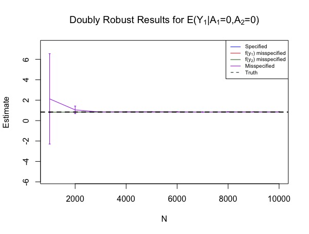
Figure 5: Performance of the doubly robust estimator estimator for $\mathbb{E}[Y_{1}(a_{1},a_{2})]$ for various values of $a_{1},a_{2}$. The purple line denotes full misspecification.

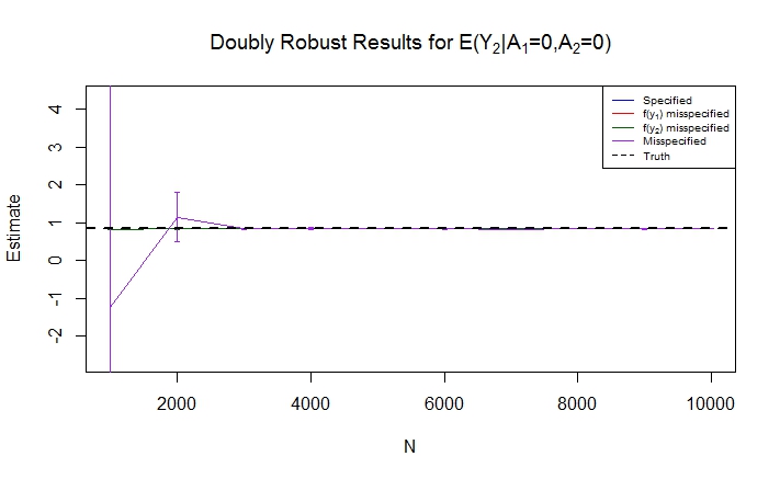
Figure 6: Performance of the doubly robust estimator estimator for $\mathbb{E}[Y_{2}(a_{1},a_{2})]$ for various values of $a_{1},a_{2}$. The purple line denotes full misspecification.

Our simulation study considered sample sizes from $1000$ to $10000$, with $50$ replicates at each sample size. For case 2, we implemented the maximum likelihood estimator in equation (26). The results are shown in Figs. 3 and 4. For case 1, we estimated $\mathbb{E}[Y_{i}(a_{1},a_{2}^{\prime})]$ using the doubly robust estimator for $\beta_{h}$ in (32) evaluated at $\beta_{y_{i}}/\beta_{1}$, and using the doubly robust estimator for $\eta(y_{1},y_{2})$ in (27) as a subroutine. The results are shown in Figs. 5 and 6 in Online Appendix 1, with Fig. 7 showing the performance of the doubly robust estimator for $\eta(y_{1},y_{2})$ used as a subroutine by the doubly robust estimators of $\mathbb{E}[Y_{i}(a_{1},a_{2})]$.

The MLE behaves as expected. The DR estimator for $\eta(y_{1},y_{2})$ behaves as expected as well. In particular, it behaves as a consistent estimator if at least one model from the set $\{f_{y^{1}},f_{y^{2}}\}$ is correctly specified. The DR estimator for $\mathbb{E}[Y(a_{1},a_{2})]$ behaves as expected for $a_{1}=0,a_{2}=1$ and $a_{1}=1,a_{2}=0$, exhibits some instability for the case of both models being misspecified for $a_{1}=a_{2}=1$, and exhibits performance robust to misspecification of both models for $a_{1}=a_{2}=0$. We believe this last behavior is due to the fact that a mixed interaction model for $h^{y^{i}}$ evaluated at $a_{1}=a_{2}=0$ cancels most of the misspecified parameters from the expression.

7 Application: The Wisconsin Longitudinal Study

We applied our derived maximum likelihood estimators to assess the spillover effect components of educational attainment on depressive symptoms in the presence of interference between spousal dyads. Our data comes from the Wisconsin Longitudinal Study (WLS), which has followed a random sample of Wisconsin-area high school graduates from the Class of 1957 for over 50 years. The WLS collected information on a wide range of socioeconomic and psychological factors, including occupation, physical and mental well-being, and health in later life. The WLS participants were interviewed roughly every 10-15 years between 1957 and 2011, with several interview questions pertaining to their spouses (if married). The WLS participants’ spouses themselves were interviewed in 2004. For further details on the WLS, we refer the reader to Herd et al. (2014). Our exposure of educational attainment $A$ was based on the 1975 WLS interview, where the participant was asked about the highest level of education completed after high school. We dichotomized responses based on a cutoff of a four year college/university degree or higher ($A=1$) versus less than a four year degree. Depressive symptoms for the WLS participant ($Y^{1}$) and his/her spouse ($Y^{2}$) was ascertained in 2003-2005, when a random 80% sample of WLS participants and their spouses were asked the question ”‘Have you ever had a time in life lasting two weeks or more when nearly every day you felt sad, blue, depressed, or when you lost interest in most things like work, hobbies, or things you usually liked to do for fun?”’ An affirmative response to this question and a negative response to a follow-up question about the depressive episode being due to alcohol, drugs, medications, or physical illness was considered evidence of depressive symptoms ($Y^{1}=1$ and/or $Y^{2}=1$); otherwise, it was assumed that depressive symptoms were absent ($Y^{1}=0$ and/or $Y^{2}=0$). In all models, we adjusted for sex, the highest educational attainment of the WLS participants’/spouses’”‘head of household”’ when he or she was 16 years old, and the Ducan Socioeconomic Status Index score of the ”‘head of household.”’ For the WLS participant, we additionally adjusted for his/her 1957 IQ score. After excluding observations for missing treatment, outcome, and/or covariate information, our analytic sample was $N=1,768$ dyads.

As a first step, we tested whether the restriction on the observed data law given in (33) held for data. Specifically, we used a Breslow-Day test to test the null hypothesis that the odds ratio for $Y^{1}$ and $Y^{2}$ was homogeneous across $A=1$ and $A=0$, and we found insufficient evidence to reject this null ($\chi^{2}=0.08$, df=1, p-value=0.77). We then estimated $\hat{\psi}(a^{\prime},a^{\prime\prime})$ given in (26) by fitting logistic regression models, allowing us to estimate the direct component of the spillover effect as $\hat{\psi}(1,0)-\hat{\psi}(0,0)$ and the indirect component as $\hat{\psi}(1,1)-\hat{\psi}(1,0)$. We obtained 95% confidence intervals by bootstrapping with 1,000 replicates. We found that the direct component of the spillover effect was -0.01 (95% CI: -0.04, 0.01), while the indirect component of the spillover effect was 0.01 (95% CI: 0.00, 0.02). Thus, since the second CI included the null before rounding, we conclude that neither component of the spillover effect is significant at the traditional $\alpha=0.05$ level. However, the direct component of the spillover effect is marginally significant. In Online Appendix 2 and 3, we provide SAS and R code to replicate the analysis.

8 Conclusions

In this paper, we proposed a new approach for decomposing the spillover effect in causal inference problems with partial interference among interacting units. We decomposed the spillover effect into direct, indirect and unit-specific components using an approach that considers outcomes to be on the same footing. In particular, our approach yields a coherent way for any one of the interacting outcomes to serve as the “outcome” for the spillover effect, with the other outcomes acting as “mediators.”

To achieve this property, we use a generalization of causal models of the DAG (Pearl, 2009) to chain graphs (Lauritzen and Richardson, 2002), which allow both directed causal relationships between treatments and outcomes, and symmetric relationships between outcomes that arise in interference problems. Given a causal chain graph model, we propose to view mediation analysis as “splitting,” or decomposition of treatments, as a generalization of the approach to mediation analysis described in Robins and Richardson (2010).

We show that under our model functionals corresponding to direct and indirect components of the spillover effects are identified via the symmetric mediation formula, and that some of the assumptions that identification relies on can be falsified from observed data. This falsifiability property is not present in mediation analysis in DAG models, and is implied by the symmetric structure of our proposed model. We describe statistical inference for components of the spillover effect in our setting. We propose two estimators, one based on maximizing the log likelihood, and one which exhibits double robustness in a restricted version of our problem.

Supplementary Materials For:
Symmetric Treatment Decomposition Of Spillover Effects

Ilya Shpitser ilyas@cs.jhu.edu
Department of Computer Science
Johns Hopkins University
Baltimore, MD 21218, USA Eric J. Tchetgen Tchetgen ett@wharton.upenn.edu
Department of Statistics
The Wharton School
3620 Locust Walk, Philadelphia, PA 19104, USA Ryan M. Andrews andrews@leibniz-bips.de
Leibniz Institute for Prevention Research and Epidemiology–BIPS
Achterstr. 30, 28359 Bremen, Germany

Appendix 1: Proofs

Lemma 4  Under the CGM associated with a CG ${\cal G}$ with a vertex set ${\vec{V}}$, the observed data distribution factorizes as

$$p({\vec{V}})=\prod_{{\vec{B}}\in{\cal B}({\cal G})}\frac{1}{Z_{\vec{B}}(\operatorname{pa}_{\cal G}({\vec{B}}))}\left(\prod_{{\vec{C}}\in{\cal C}(({\cal G}_{\operatorname{fa}_{\cal G}({\vec{B}})})^{a}),{\vec{C}}\not\subseteq\operatorname{pa}_{\cal G}({\vec{B}})}\phi_{\vec{C}}({\vec{C}})\right),$$

where $\phi_{\vec{C}}({\vec{C}})$ are unnormalized potential functions mapping ${\mathfrak{X}}_{\vec{C}}$ to real numbers.

Proof  If ${\cal G}$ is complete, the result is a generalization of results in (Richardson and Robins, 2013). If ${\cal G}$ is an edge subgraph of a complete CG ${\cal G}^{*}$, then $p({\vec{B}}(\vec{a}_{\vec{B}}))=p({\vec{B}}\mid\operatorname{pa}_{\cal G}({\vec{B}})=\vec{a}_{\vec{B}})$, and (16) gives exactly the local Markov property for chain graphs for ${\cal G}$. Since we assumed positivity for every factor, $p({\vec{V}})$ is positive, and local Markov property implies that $p({\vec{V}})$ obeys the chain graph factorization with respect to ${\cal G}$, which gives our conclusion.  

Lemma 5  For any valid $\vec{A}$ in a CGM associated with a CG ${\cal G}$ with vertex set ${\vec{V}}$, if $\left(\prod_{\vec{B}\in{\cal B}({\cal G});\vec{B}\subseteq\vec{A}}p(\vec{B}\mid\operatorname{pa}_{\cal G}(\vec{B}))\right)>0$, almost surely,

$$p(\{{\vec{V}}\setminus\vec{A}\}(\vec{a})={\vec{v}})=\prod_{{\vec{B}}\in{\cal B}({\cal G}),{\vec{B}}\cap\vec{A}=\emptyset}\frac{\prod_{{\vec{C}}\in{\cal C}(({\cal G}_{\operatorname{fa}_{\cal G}({\vec{B}})})^{a},{\vec{C}}\not\subseteq\operatorname{pa}_{\cal G}({\vec{B}}))}\phi_{\vec{C}}(\vec{a}_{{\vec{C}}\cap\vec{A}},{\vec{v}}_{{\vec{C}}\setminus\vec{A}})}{Z_{\vec{B}}(\vec{a}_{\vec{A}\cap\operatorname{pa}_{\cal G}({\vec{B}})},{\vec{v}}_{\operatorname{pa}_{\cal G}({\vec{B}})\setminus\vec{A}})}.$$ (38)

Similarly, for a subset $\vec{Y}\subset{\vec{V}}\setminus\vec{A}$,

$$p(\vec{Y}(\vec{a})={\vec{v}}_{\vec{Y}})=\sum_{{\vec{v}}_{{\vec{V}}\setminus(\vec{Y}\cup\vec{A})}}\prod_{{\vec{B}}\in{\cal B}({\cal G}),{\vec{B}}\cap\vec{A}=\emptyset}\frac{\prod_{{\vec{C}}\in{\cal C}(({\cal G}_{\operatorname{fa}_{\cal G}({\vec{B}})})^{a},{\vec{C}}\not\subseteq\operatorname{pa}_{\cal G}({\vec{B}}))}\phi_{\vec{C}}(\vec{a}_{{\vec{C}}\cap\vec{A}},{\vec{v}}_{{\vec{C}}\setminus\vec{A}})}{Z_{\vec{B}}(\vec{a}_{\vec{A}\cap\operatorname{pa}_{\cal G}({\vec{B}})},{\vec{v}}_{\operatorname{pa}_{\cal G}({\vec{B}})\setminus\vec{A}})}.$$ (39)

Proof  This follows by the generalization of the argument proving propositions 11 and 16 in (Richardson and Robins, 2013) from singleton nodes to blocks. Note that restricting attention to the “outer” factorization of a CG resembling the DAG factorization defined on elements of ${\cal B}({\cal G})$ suffices for the argument. A generalization which allows for interventions on a strict subset of a block is given in (Lauritzen and Richardson, 2002).  

Lemma 6  Fix an arbitrary value assignment $\tilde{a}$ to $\tilde{A}\equiv\{\tilde{A}^{1},\ldots\tilde{A}^{N}\}$. Then under consistency, positivity, conditional ignorability, and (23),

$$p(Y^{i}(\tilde{a})=y^{i}) =\sum_{c,y^{(i)}}\frac{\left(\prod_{j=1}^{N}\phi_{Y^{j},\tilde{A}^{j}}(y^{j},\tilde{a}^{j})\right)\prod_{S\in{\cal C}({\cal G}_{\vec{Y}})}\phi_{S}(\vec{y}_{S})}{Z(\tilde{a},c)}p(c),$$ (40)

where $\vec{y}_{C}$ is the subset of $\vec{y}$ pertaining to $S$. Note that $\tilde{a}$ may potentially assign conflicting values to different components of $A$ in $\tilde{A}$. As a result, Lemma 5 cannot be used directly to obtain identification, since the positivity assumption $\left(\prod_{\vec{B}\in{\cal B}({\cal G});\vec{B}\subseteq\tilde{A}}p(\vec{B}\mid\operatorname{pa}_{\cal G}(\vec{B}))\right)>0$ made in that Lemma does not hold. In particular, in all realizations of the observed data distribution, the same values are assigned to all elements in $\tilde{A}$. Nevertheless, assumptions (23) may be used to get around this.

Proof  If positivity does hold, $p(Y^{i}(\tilde{a})=y^{i})$ is identified by (40). This follows from the fact that if conditional ignorability and (23) hold, they yield the CGM corresponding to the outcome-specific extended treatment CG. Identifying functional (40) then follows by Lemma 5. The fact that this functional may be estimated from data which does not contain conflicting realizations $\tilde{a}^{i}\neq\tilde{a}^{j}$ for any $i,j$ follows from the fact that each element of the CG factorization in the functional contains at most a single value of elements in $\tilde{A}$.  

Finally, we prove that the solution $\widetilde{\beta}_{h,dr}$ to the estimating equation described in section 6.2 is doubly robust in the sense of being consistent under the union model where either (i) and (ii.a) or (i) and (ii.b) from section 6.2 hold. Note that under (i) and (ii), $\widehat{\nu}_{dr}$ is consistent. Furthermore, suppose that (ii.a) holds such that $\widetilde{\omega}_{1}(\widehat{\nu}_{dr})$ is also consistent. Note that under this submodel $\widetilde{\beta}_{h,1}$ is consistent but $\widetilde{\beta}_{h,2}$ is consistent for

$$\sum_{y^{1},y^{2}}f(y^{1}|a{{}^{\prime}},Y^{2}=0;\omega_{1})h(y^{1},y^{2})f(y^{2}|a{{}^{\prime\prime}},Y^{1}=0;\omega_{2}^{\ast})\gamma(y_{i}^{1},y^{2};\nu).$$

Then for all $\omega_{2}^{\ast}$,

$$E\left\{U_{dr,i}(h;\beta_{h},\omega_{1},\omega_{2}^{\ast})|a_{i},y_{i}^{1}\right\}$$

$$\propto \!\!\!\!\!\sum_{y^{1}}\frac{\gamma(y^{1},y_{i}^{2})f(y_{i}^{1}|a{{}^{\prime}},Y^{2}=0)}{\gamma(y^{1},y_{i}^{2}|\nu)}$$

$$\!\!\!\!\!\times\left\{\begin{array}[]{c}\gamma(y^{1},y^{2};\nu)h(y^{1},y_{i}^{2})-\beta_{h}(a{{}^{\prime}},a{{}^{\prime\prime}})\\ -\sum_{y^{1}}h(y^{1},y_{i}^{2})f(y^{1}|a{{}^{\prime}},Y_{i}^{2}=0,\omega_{1})\gamma(y^{1},y_{i}^{2};\nu)+\beta_{h}(a{{}^{\prime}},a{{}^{\prime\prime}})\\ -\sum_{y^{2}}h(y^{1},y^{2})f(y^{2}|a{{}^{\prime\prime}},Y^{1}=0,\omega_{2}^{\ast})\gamma(y^{1},y^{2};\nu)+\beta_{h,2}^{\ast}(a{{}^{\prime}},a{{}^{\prime\prime}})\end{array}\right\}$$

$$= \!\!\!\!\!\left\{\begin{array}[]{c}\sum_{y^{1}}f(y^{1}|a{{}^{\prime}},Y^{2}=0;\omega_{1})\gamma(y^{1},y_{i}^{2};\nu)h(y^{1},y_{i}^{2})-\beta_{h}(a{{}^{\prime}},a{{}^{\prime\prime}})\\ -\sum_{y^{1}}h(y^{1},y_{i}^{2})f(y^{1}|a{{}^{\prime}},Y_{i}^{2}=0;\omega_{1})\gamma(y^{1},y_{i}^{2};\nu)+\beta_{h}(a{{}^{\prime}},a{{}^{\prime\prime}})\\ \underset{=0}{\underbrace{-\sum_{y^{1},y^{2}}\!\!f(y^{1}|a{{}^{\prime}},Y^{2}=0)h(y^{1},y^{2})f(y^{2}|a{{}^{\prime\prime}},Y^{1}=0;\omega_{2}^{\ast})\gamma(y_{i}^{1},y^{2};\nu)+\beta_{h,2}^{\ast}(a{{}^{\prime}},a{{}^{\prime\prime}})}}\end{array}\right\}$$

$$= \!\!\!\!\!0.$$

Next, suppose that (i) and (ii.b) hold. Then $\widetilde{\beta}_{h,2}$ is consistent but $\widetilde{\beta}_{h,1}$ is consistent for

$$\sum_{y^{1},y^{2}}f(y^{1}|a{{}^{\prime}},Y^{2}=0;\omega_{1}^{\ast})h(y^{1},y^{2})f(y^{2}|a{{}^{\prime\prime}},Y^{1}=0;\omega_{2})\gamma(y_{i}^{1},y^{2};\nu).$$

Then for all $\omega_{1}^{\ast}$,

$$\!\!\!\!\!E\left\{U_{dr,i}(h;\beta_{h},\omega_{1}^{\ast},\omega_{2})|a_{i},y_{i}^{1}\right\}$$

$$\propto \sum_{y^{2}}\frac{\gamma(y_{i}^{1},y^{2})f(y^{2}|a{{}^{\prime}},Y^{1}=0)\ f(y^{2}|a{{}^{\prime\prime}},Y^{1}=0;\omega_{2})}{\gamma(y^{1},y_{i}^{2};\nu)f(y^{2}|a{{}^{\prime}},Y^{1}=0;\omega_{2})}$$

$$\!\!\!\!\!\times\left\{\begin{array}[]{c}\gamma(y_{1}^{1},y^{2};\nu)h(y_{1}^{1},y^{2})-\beta_{h}(a{{}^{\prime}},a{{}^{\prime\prime}})\\ -\sum_{y^{1}}h(y^{1},y^{2})f(y^{1}|a{{}^{\prime}},Y_{i}^{2}=0;\omega_{1}^{\ast})\gamma(y^{1},y^{2};\nu)+\beta_{h,1}^{\ast}(a{{}^{\prime}},a{{}^{\prime\prime}},{\vec{c}}_{i})\\ -\sum_{y^{2}}h(y_{i}^{1},y^{2})f(y^{2}|a{{}^{\prime\prime}},Y^{1}=0;\omega_{2})\gamma(y_{i}^{1},y^{2}|\nu)+\beta_{h}(a{{}^{\prime}},a{{}^{\prime\prime}},{\vec{c}}_{i};\kappa)\end{array}\right\}$$

$$= \!\!\!\!\!\left\{\begin{array}[]{c}\sum_{y^{1}}f(y^{2}|a{{}^{\prime}},Y^{1}=0)\gamma(y^{1},y^{2};\nu)h(y^{1},y^{2})-\beta_{h}(a{{}^{\prime}},a{{}^{\prime\prime}})\\ -\sum_{y^{1},y^{2}}\ f(y^{2}|a{{}^{\prime\prime}},Y^{1}=0;\omega_{2})h(y^{1},y^{2})f(y^{1}|a{{}^{\prime}},Y_{i}^{2}=0;\omega_{1}^{\ast})\gamma(y^{1},y^{2};\nu)\\ +\beta_{h,1}^{\ast}(a{{}^{\prime}},a{{}^{\prime\prime}})-\sum_{y^{2}}h(y_{i}^{1},y^{2})f(y^{2}|a{{}^{\prime\prime}},Y^{1}=0,{\vec{c}}_{i};\omega_{2})\gamma(y_{i}^{1},y^{2}|{\vec{c}}_{i};\nu)+\beta_{h}(a{{}^{\prime}},a{{}^{\prime\prime}})\end{array}\right\}$$

$$= \!\!\!\!\!0,$$

proving the result.

Appendix 2: Figures

Figure 3: Performance of the maximum likelihood estimator for $\mathbb{E}[Y_{1}(a_{1},a_{2})]$ for various values of $a_{1},a_{2}$.

Figure 4: Performance of the maximum likelihood estimator for $\mathbb{E}[Y_{2}(a_{1},a_{2})]$ for various values of $a_{1},a_{2}$.

Figure 7: Performance of the doubly robust estimator estimator for $\eta(Y_{1},Y_{2})$ used as a subroutine by the doubly robust estimators for $\mathbb{E}[Y_{i}(a_{1},a_{2})]$. The purple line denotes full misspecification.

Appendix 3: SAS code

The following SAS code assumes that the Wisconsin Longitudinal Study (WLS) data has been downloaded from https://www.ssc.wisc.edu/wlsresearch/data/.

In particular, we make use of the ”marriage” dataset that contains information on each participant and his/her spouse, as well as the ”long” version of the main WLS data. Text in brackets should be replaced to map to your own file library locations.

⬇

OPTIONS nofmterr;

data marriage noformats;

set [marriage].public_grad_marriage_roster_long;

keep=idpub cmdeath cmspdth cmstart mar_num;

run;

data wls_long;

set [long].wls_bl_13_07 (where=(rtype="g")

keep=idpub rtype z_dglev z_brdxdy z_sexrsp

z_hcb10sp z_hc012sp z_hc013sp z_hb005rec

z_gu002re z_gu003re z_gu004re z_au002re

z_au003re z_au004re gwiiq_bm z_aa003re

edsphh ocssphu z_edhhyr z_ocsh57u2 z_aa001re;

run;

proc sql;

create table wls_select AS SELECT

* FROM

wls_long INNER JOIN

marriage on wls_long.idpub = marriage.idpub;

quit;

PROC EXPORT DATA=wls_select

FILE="[output.dta]"

DBMS=STATA REPLACE;

RUN;

Appendix 4: R code

⬇

library(haven)

library(dplyr)

library(readr)

library(boot)

library(DescTools)

#Required: output.dta from Appendix 3

wls_data_select <- read_dta("[output.dta]") %>%

transmute(idpub,

rtype,

grad_female = ifelse(z_sexrsp==2, 1, 0),

graduate_birth_year = z_brdxdy + 1900,

education_spouse = z_hcb10sp,

spouse_age_2011=z_hc012sp,

spouse_age_marriage=z_hc013sp,

education_graduate = z_dglev,

mar_num,

graduate_death_year = cmdeath,

spouse_death_year = cmspdth,

marriage_year = cmstart,

z_gu002re,

z_gu003re,

graduate_age_depressed = z_gu004re,

z_au002re,

z_au003re,

spouse_age_depressed = z_au004re,

edsphh,

gwiiq_bm,

ocssphu,

z_edhhyr,

z_ocsh57u2,

z_aa001re

) %>%

mutate(spouse_age_death = ifelse(spouse_death_year > 0, spouse_death_year - (marriage_year - spouse_age_marriage), NA),

graduate_age_death = ifelse(graduate_death_year > 0, graduate_death_year - graduate_birth_year, NA),

spouse_dead = ifelse(spouse_death_year > 0, 1, 0),

graduate_dead = ifelse(graduate_death_year >0, 1, 0),

spouse_college = case_when(

is.na(education_spouse)==1 ~ NA_real_,

education_spouse <= 0 ~ NA_real_,

education_spouse >=16 & education_spouse <= 26 ~ 1,

education_spouse == 32 ~ 0,

education_spouse == 35 ~ 0,

education_spouse == 40 ~ 0,

education_spouse >= 45 ~ 1,

TRUE ~ 0

),

graduate_college = case_when(

is.na(education_graduate) ~ NA_real_,

education_graduate < 2 ~ 0,

education_graduate >= 2 ~ 1

),

graduate_depressed = case_when(

is.na(z_gu002re) == 1 ~ NA_real_,

z_gu002re < 0 ~ NA_real_,

z_gu002re == 1 ~ 1,

z_gu002re == 2 ~ 0,

TRUE ~ 0

),

spouse_depressed = case_when(

is.na(z_au002re) == 1 ~ NA_real_,

z_au002re < 0 ~ NA_real_,

z_au002re == 1 ~ 1,

z_au002re == 2 ~ 0,

TRUE ~ 9999

),

graduate_depressed_reason = case_when(

is.na(z_gu003re) == 1 ~ NA_real_,

z_gu003re == 1 | z_gu003re ==2 ~ 1,

z_gu003re == 3 ~ 0,

z_gu003re < 0 ~ 0,

TRUE ~ 9999),

spouse_depressed_reason = case_when(

is.na(z_au003re) == 1 ~ NA_real_,

z_au003re == 1 | z_au003re ==2 ~ 1,

z_au003re == 3 ~ 0,

z_au003re < 0 ~ 0,

TRUE ~ 9999),

educ_spouse_hoh = case_when(

edsphh < 0 ~ NA_real_,

edsphh >=0 & edsphh <= 11 ~ 0,

edsphh >= 12 & edsphh < 16 ~ 1,

edsphh >=16 ~ 2),

gwiiq_bm,

duncan_sei_spouse = case_when(

ocssphu < 0 ~ NA_real_,

TRUE ~ ocssphu),

educ_grad_hoh = case_when(

z_edhhyr < 0 ~ NA_real_,

z_edhhyr > 0 & z_edhhyr <=11 ~ 0,

(z_edhhyr >=12 & z_edhhyr < 16) | z_edhhyr == 32 ~ 1,

z_edhhyr >= 16 ~ 2),

duncan_sei_grad = case_when(

z_ocsh57u2 < 0 ~ NA_real_,

TRUE ~ z_ocsh57u2),

spouse_female = case_when(

z_aa001re == 1 ~ 0,

z_aa001re == 2 ~ 1,

TRUE ~ NA_real_

))

analytic <- wls_data_select %>%

filter(is.na(spouse_college)==0 & is.na(graduate_college)==0) %>%

filter(is.na(marriage_year)==0) %>%

filter(is.na(spouse_age_marriage)==0) %>%

filter(is.na(graduate_depressed)==0 & is.na(spouse_depressed)==0) %>%

filter(graduate_depressed_reason == 0 & spouse_depressed_reason == 0)

analytic2 <- analytic %>%

dplyr::select(graduate_depressed,

spouse_depressed,

graduate_college,

educ_spouse_hoh,

duncan_sei_spouse,

educ_grad_hoh,

duncan_sei_grad,

spouse_female,

grad_female,

gwiiq_bm) %>%

filter(complete.cases(.))

#Test the observed data law restriction

bin_table <- table(analytic2$graduate_depressed,

analytic2$spouse_depressed,

analytic2$graduate_college,

dnn=c(’graduate_depressed’, ’spouse_depressed’,’graduate_college’))

bin_table

BreslowDayTest(bin_table)

#Define functions for later use

y1_model = as.formula(graduate_depressed ~ graduate_college + gwiiq_bm + grad_female + duncan_sei_grad + educ_grad_hoh)

y2_model = as.formula(spouse_depressed ~ graduate_college + spouse_female + duncan_sei_spouse + educ_spouse_hoh)

#Function for f pdfs

pred_prob_y <- function(data, formula, outcome, trt_comp){

if(outcome=="Y1"){

dat <- data %>% filter(spouse_depressed==0)

dat_fy <- data %>% mutate(graduate_college=trt_comp, spouse_depressed=0)

}

if(outcome=="Y2"){

dat <- data %>% filter(graduate_depressed==0)

dat_fy <- data %>% mutate(graduate_college=trt_comp, graduate_depressed=0)

}

logistic_mod <- glm(formula,

data=dat,

family=binomial(link="logit"))

pred_prob = predict(logistic_mod, dat_fy, type="response")

return(pred_prob)

}

#OR function, i.e., gamma(y1,y2|c).

#Note: gamma doesn’t depend on A (only on C), so graduate_college omitted from gamma(y1,y2|c) model

gammay1y2 <- function(data, y1val, y2val, y1mod=as.formula(graduate_depressed ~ gwiiq_bm + grad_female + duncan_sei_grad + educ_grad_hoh)){

y1ref <- abs(y1val-1)

y2ref <- abs(y2val-1)

logistic_y1y2 <- glm(y1mod,

data = data[data$spouse_depressed==y2val,],

family=binomial(link="logit"))

logistic_y1y2ref <- glm(y1mod,

data = data[data$spouse_depressed==y2ref,],

family=binomial(link="logit"))

dat_y1y2 <- mutate(data, spouse_depressed==y2val)

dat_y1y2ref <- mutate(data, spouse_depressed==y2ref)

if(y1ref==0){

pr_y1y2 <- predict(logistic_y1y2,dat_y1y2, type="response")

pr_y1y2ref <- predict(logistic_y1y2ref, dat_y1y2ref, type="response")

} else{

pr_y1y2 <- 1-predict(logistic_y1y2,dat_y1y2, type="response")

pr_y1y2ref <- 1-predict(logistic_y1y2ref, dat_y1y2ref, type="response")

}

gamma <- (pr_y1y2*(1-pr_y1y2ref)) / ((1-pr_y1y2)*pr_y1y2ref)

return(gamma)

}

#Function for \psi(a1,a2) = E{Y1(a1,a2)}

EYa1a2 <- function(data, h, fy1, fy2){

numer_EY <- (h*fy1*gammay1y2(data, y1val=1, y2val=1)*fy2) + (h*fy1*gammay1y2(data, y1val=1, y2val=0)*(1-fy2))

denom_EY <- (fy1*gammay1y2(data, y1val=1, y2val=1)*fy2) + ((1-fy1)*gammay1y2(data, y1val=0, y2val=1)*fy2) + (fy1*gammay1y2(data, y1val=1, y2val=0)*(1-fy2)) + ((1-fy1)*gammay1y2(data, y1val=0, y2val=0)*(1-fy2))

EY <- mean(numer_EY/denom_EY)

return(EY)

}

DE_estimate <- function(d, indices, y1_model, y2_model){

data <- d[indices,]

fy1_a1eq1 <- pred_prob_y(data=data, formula=y1_model, outcome = "Y1", trt_comp=1)

fy2_a2eq0 <- pred_prob_y(data=data, formula=y2_model, outcome = "Y2", trt_comp=0)

EY10 <- EYa1a2(data, h=1, fy1 = fy1_a1eq1, fy2 = fy2_a2eq0)

fy1_a1eq0 <- pred_prob_y(data=data, formula=y1_model, outcome = "Y1", trt_comp=0)

EY00 <- EYa1a2(data, h=1, fy1 = fy1_a1eq0, fy2 = fy2_a2eq0)

DE = EY10 - EY00

return(DE)

}

IE_estimate <- function(d, indices, y1_model, y2_model){

data <- d[indices,]

fy1_a1eq1 <- pred_prob_y(data=data, formula=y1_model, outcome = "Y1", trt_comp=1)

fy2_a2eq0 <- pred_prob_y(data=data, formula=y2_model, outcome = "Y2", trt_comp=0)

EY10 <- EYa1a2(data, h=1, fy1 = fy1_a1eq1, fy2 = fy2_a2eq0)

fy2_a2eq1 <- pred_prob_y(data=data, formula=y2_model, outcome = "Y2", trt_comp=1)

EY11 <- EYa1a2(data, h=1, fy1 = fy1_a1eq1, fy2 = fy2_a2eq1)

IE = EY11 - EY10

return(IE)

}

set.seed(1234)

DE_boot <- boot(data=analytic2, statistic = DE_estimate, R=1e3, y1_model=y1_model, y2_model=y2_model)

DE_CI <- boot.ci(DE_boot, type=’perc’)

IE_boot <- boot(data=analytic2, statistic= IE_estimate, R=1e3, y1_model=y1_model, y2_model=y2_model)

IE_CI <- boot.ci(IE_boot, type=’perc’)

print(paste0(’non-DR␣DE␣estimate:’, ’␣’, round(DE_CI$t0, 3), ’␣’, ’(’, round(DE_CI$percent[4],3), ’,␣’, round(DE_CI$percent[5],3), ’)’ ))

print(paste0(’non-DR␣IE␣estimate:’, ’␣’, round(IE_CI$t0, 3), ’␣’, ’(’, round(IE_CI$percent[4],3), ’,␣’, round(IE_CI$percent[5],3), ’)’ ))

References

- Baron and Kenny (1986) Reuben M. Baron and David A. Kenny. The moderator-mediator variable distinction in social psychology research: Conceptual, strategic, and statistical considerations. Journal of Personality and Social Psychology, 51:1173–1182, 1986.
- Besag (1975) Julian Besag. Statistical analysis of lattice data. The Statistician, 24(3):179–195, 1975.
- Chen (2007) Hua Yun Chen. A semiparametric odds ratio model for measuring association. biometrics, 63:413–421, 2007.
- Cox and Wermuth (1993) D. R. Cox and N. Wermuth. Linear dependencies represented by chain graphs. Statistical Science, 8(3):204–283, 1993.
- Halloran and Struchiner (1995) M. Elizabeth Halloran and C. J. Struchiner. Causal inference for infectious diseases. Epidemiology, 6:142–151, 1995.
- Herd et al. (2014) Pamela Herd, Deborah Carr, and Carol Roan. Cohort profile: Wisconsin longitudinal study (wls). International journal of epidemiology, 43(1):34–41, 2014.
- Hojsgaard et al. (2012) Soren Hojsgaard, David Edwards, and Steffen Lauritzen. Graphical Models with R. Springer-Verlag New York, 1st edition edition, 2012.
- Hudgens and Halloran (2008) M.G. Hudgens and M.E. Halloran. Toward causal inference with interference. Journal of the American Statistical Association, 103(482):832–842, 2008.
- Lauritzen (1996) Steffan L. Lauritzen. Graphical Models. Oxford, U.K.: Clarendon, 1996.
- Lauritzen and Richardson (2002) Steffen L. Lauritzen and Thomas S. Richardson. Chain graph models and their causal interpretations (with discussion). Journal of the Royal Statistical Society: Series B, 64:321–361, 2002.
- Neyman (1923) Jerzy Neyman. Sur les applications de la thar des probabilities aux experiences agaricales: Essay des principle. excerpts reprinted (1990) in English. Statistical Science, 5:463–472, 1923.
- Ogburn and VanderWeele (2014) Elizabeth L. Ogburn and Tyler J. VanderWeele. Causal diagrams for interference. Statistical Science, 29(4):559–578, 2014.
- Pearl (1988) Judea Pearl. Probabilistic Reasoning in Intelligent Systems. Morgan and Kaufmann, San Mateo, 1988.
- Pearl (2001) Judea Pearl. Direct and indirect effects. In Proceedings of the Seventeenth Conference on Uncertainty in Artificial Intelligence (UAI-01), pages 411–420. Morgan Kaufmann, San Francisco, 2001.
- Pearl (2009) Judea Pearl. Causality: Models, Reasoning, and Inference. Cambridge University Press, 2 edition, 2009. ISBN 978-0521895606.
- Pearl (2011) Judea Pearl. The causal mediation formula – a guide to the assessment of pathways and mechanisms. Technical Report R-379, Cognitive Systems Laboratory, University of California, Los Angeles, 2011.
- Richardson and Robins (2013) Thomas S. Richardson and Jamie M. Robins. Single world intervention graphs (SWIGs): A unification of the counterfactual and graphical approaches to causality. preprint: http://www.csss.washington.edu/Papers/wp128.pdf, 2013.
- Robins (1986) James M. Robins. A new approach to causal inference in mortality studies with sustained exposure periods – application to control of the healthy worker survivor effect. Mathematical Modeling, 7:1393–1512, 1986.
- Robins and Greenland (1992) James M. Robins and Sander Greenland. Identifiability and exchangeability of direct and indirect effects. Epidemiology, 3:143–155, 1992.
- Robins and Richardson (2010) James M. Robins and Thomas S. Richardson. Alternative graphical causal models and the identification of direct effects. Causality and Psychopathology: Finding the Determinants of Disorders and their Cures, 2010.
- Rubin (1976) D. B. Rubin. Causal inference and missing data (with discussion). Biometrika, 63:581–592, 1976.
- Shpitser (2013) Ilya Shpitser. Counterfactual graphical models for longitudinal mediation analysis with unobserved confounding. Cognitive Science (Rumelhart special issue), 37:1011–1035, 2013.
- Shpitser and Pearl (2006a) Ilya Shpitser and Judea Pearl. Identification of joint interventional distributions in recursive semi-Markovian causal models. In Proceedings of the Twenty-First National Conference on Artificial Intelligence (AAAI-06). AAAI Press, Palo Alto, 2006a.
- Shpitser and Pearl (2006b) Ilya Shpitser and Judea Pearl. Identification of conditional interventional distributions. In Proceedings of the Twenty Second Conference on Uncertainty in Artificial Intelligence (UAI-06), pages 437–444. AUAI Press, Corvallis, Oregon, 2006b.
- Shpitser and Tchetgen Tchetgen (2016) Ilya Shpitser and Eric J. Tchetgen Tchetgen. Causal inference with a graphical hierarchy of interventions. Annals of Statistics, 44(6):2433–2466, 2016.