A model of the effect of collisions on QCD plasma instabilities

Collective excitations of a hot anisotropic QCD medium with Bhatnagar-Gross-Krook collisional kernel within an effective description

Abstract

Collective modes of an anisotropic hot QCD medium have been studied within the semi-classical transport theory employing Bhatnagar-Gross-Krook (BGK) collisional kernel. The modeling of the isotropic medium is primarily based on a recent quasi-particle description of hot QCD equation of state where the medium effects have been encoded in effective gluon and quark/anti-quark momentum distributions that posses non-trivial energy dispersions. The anisotropic distribution functions are obtained in a straightforward the way by stretching or squeezing the isotropic ones along one of the directions. The gluon self-energy is computed using these distribution functions in a linearized transport equation with Bhatnagar-Gross-Krook (BGK) collisional kernel. Further, the tensor decomposition of gluon self-energy leads to the structure functions which eventually controls the dispersion relations and the collective mode structure of the medium. It has been seen that both the medium effects and collisions induce appreciable modifications to the collective modes and plasma excitations in the hot QCD medium.

Keywords: Collective modes, BGK collisional kernel, Anisotropic QCD, Quark-Gluon-Plasma, Quasi-partons, Gluon self-energy.

PACS: 12.38.Mh, 13.40.-f, 05.20.Dd, 25.75.-q

I Introduction

The matter at extreme conditions of temperature/energy density behaves more like a near perfect fluid with the smallest value of the shear viscosity to entropy ratio among almost all the known fluids in nature. This fact is strongly supported by the experimental observations at RHIC, BNL expt_rhic , and LHC, CERN expt_lhc . In particular, the robust collective flow phenomenon and strong jet quenching both at RHIC and LHC indicate towards the strongly coupled nature of this medium which is commonly termed as quark-gluon-plasma (QGP). Also, theoretical investigations based on various approaches starting from kinetic theory to holographic theories also hint towards a tiny value for the shear viscosity to entropy density ratio for the QGP/hot QCD matter Ryu ; Denicol1 .

Among a few other interesting observations, suppression of quarkonia yields at high transverse momentum observed in these experiments highlight the plasma aspects of the medium such a color screening Chu:1988wh , landau damping Landau:1984 and energy loss Koike:1991mf . In a hot QCD medium/QGP, such aspects can be explored in terms of gluon polarization tensor or self-energy of the medium that helps in exploring the spectrum of the collective excitations of the medium. The collective excitations carry crucial information about the equilibrated QGP and also provide an information on the temporal evolution of the non (near)-equilibrated one. In the present manuscript, a collisional anisotropic QGP is considered where the collisions are governed by BGK kernel. The prime reason to consider the anisotropy (momentum) is due to the fact that it has been there in all the stages of heavy-ion collisions. The BGK collision kernel ensures the local number/current conservation. Therefore, it is always wise to consider BGK over the RTA (relaxation-time -approximation) while incorporating the collision in the theory.

The collective excitations of the hot QCD medium have been studied by several groups Mrowczynski:1993qm ; Mrowczynski:1994xv ; Mrowczynski:1996vh ; Jamal:2017dqs ; avdhesh . The results are obtained either by employing linearized semi-classical transport theory or Hard-Thermal-Loop (HTL) effective theory upto one-loop in weak coupling limit. The two approaches reached to the same results dm_rev1 ; dm_rev2 ; Mrowczynski:2000ed ; Mrowczynski:2004kv for the gluon self-energy and collective modes. Apart from that there have been a few works where the collisional aspects of the QGP have been included either with RTA Akamatsu:2013pjd or BGK collision term Bhatnagar:1954 ; Jiang:2016dkf ; Schenke:2006xu while considering isotropic as well as anisotropic aspects of the medium. In either of the approaches, the dispersion equations are obtained from the gluon polarization tensor depicting the conditions that reflects the existence of solutions of the homogeneous equation of motion (the Yang-Mills equations).

It is important to note that the hot QCD plasma (in the abelian limit) do possess collective excitations  Weibel:1959zz that could be seen as a straightforward generalization of hot QED plasma ( the difference is only in the effective coupling constant). The collective excitations (gluonic collective modes) that are commonly termed as plasmons have been investigated in isotropic/anisotropic hot QCD medium in Refs.  Romatschke:2003ms ; Romatschke:2004jh ; Mrowczynski:2005ki ; Arnold:2003rq . The distribution functions for partons employed to explore different aspects of QGP are briefly discussed in Attems:2012js ; Florkowski:2012as ; Dumitru:2007hy ; Martinez:2008di ; Schenke:2006yp . In most of these studied, QGP has been considered as the ultra-relativistic non-interacting gas of quarks, anti-quarks, and gluons which is certainly not desired because of the strongly coupled nature of QGP in experiments.

The present analysis is the extension of the work in Ref. Jamal:2017dqs , where the collective excitations of collision-less anisotropic plasma for the different equations of state(EoSs) have been studied. We shall focus on the effect of collisions by incorporating the BGK collisional kernel. It is important to mention that in Ref. Schenke:2006xu the author also have studied the collective modes of anisotropic QGP in presence of BGK collisional kernel. However, they have analyzed only the those modes which are propagating in the direction of anisotropy vector. In their analysis of zeros of the propagator they found two modes of propagation, out of which one can be unstable. The main purpose of our analysis is to study this situation with more generality. We allow the modes to propagate in all possible directions with respect to anisotropy vector. Apart from that, we also consider the effective description of the hot QCD medium within the framework of effective fugacity quasi-particle model (EQPM). In the small anisotropy limit, while considering all the possible directions of propagation with respect to anisotropy vector, we find that there exists three modes. Out of these modes, two can be unstable. We also showed that the effect of lattice and HTL inspired non-ideal EoSs can also significantly change the dispersion characteristic. Whenever possible, we have compared our results with those of in Ref. Schenke:2006xu .

The main work of the present manuscript includes, (i) detailed analysis of the stable as well as unstable modes and their dependencies on wave vector, strength of anisotropy and collisional frequency, (ii) studying small anisotropy with full angular dependence, (iii) the critical dependence of unstable modes on the collisional frequency, the angle between the propagation vector and anisotropy direction, wave vector has been investigated by obtaining their maximum allowed values while fixing the other two respectively for various values for anisotropy parameter.

The paper is organized as follows. In section  II, We shall give a brief derivation of gluon self-energy while considering the BGK collisional kernel. The modeling of hot QCD medium for the isotropic case as well as the anisotropic case is shown in the sub-section II.1. A simple decomposition of gluon self-energy in terms of structure functions and their forms in weak anisotropy limit will be presented in the different sub-sections II.2. In section III, we shall give a brief mathematical structure of the dispersion relations which we used to study different collective modes. Section IV contains the discussions of results. In section V, we offer the summary and conclusions of the present work as well as the possible future aspects.

II Gluon self-energy/polarization tensor in QCD plasma with BGK collisional kernel

Gluon self-energy/polarization tensor ($\Pi^{\mu\nu}$) carries the information of QCD medium as it describes the interactions term in the effective action of QCD. We are interested here in obtaining the expression for $\Pi^{\mu\nu}$ in the presence of collisions. To start our calculation, we shall focus on the physics at soft scale, $k\sim gT\ll T$, $g$ is the strong coupling constant. At this scale, we can assume the strength of field fluctuations, $A$ to be O($\sqrt{g}T$), and the derivatives $\partial_{x}$ of O($gT$). Applying this power counting scheme we can restrict ourself to the abelian limit by neglecting the non-abelian term. This is because in the field strength tensor, $F^{\mu\nu}=\partial^{\mu}A^{\nu}-\partial^{\nu}A^{\mu}-ig\left[A^{\mu},A^{\nu}\right]$, the order of the non-abelian term is O($g^{2}$) which is smaller than the order O($g^{3/2}$) of first two term in $F^{\mu\nu}(x)$.

In the abelian limit, the linearized semi-classical transport equations, also given in refs.Mrowczynski:1993qm -Romatschke:2003ms , can be written separately for each color channelJiang:2016dkf ; Schenke:2006xu as,

$$v^{\mu}\partial_{\mu}\delta f^{i}_{a}(p,X)+g\theta_{i}v_{\mu}F^{\mu\nu}_{a}(X)\partial_{\nu}^{(p)}f^{i}(\mathbf{p})=\mathcal{C}^{i}_{a}(p,X),$$

(1)

where, $x^{\mu}=(t,\mathbf{x})=X$ and $v^{\mu}=(1,\mathbf{v})=V$, are the four space-time coordinate and the velocity of the plasma particle, respectively with $\mathbf{v}=\mathbf{p}/|\mathbf{p}|$. $\theta_{i}\in\{\theta_{g},\theta_{q},\theta_{\bar{q}}\}$ and have the values $\theta_{g}=\theta_{q}=1$ and $\theta_{\bar{q}}=-1$. $\partial_{\mu}$, $\partial_{\nu}^{(p)}$ are the partial four derivatives corresponding to space and momentum respectively. $\mathcal{C}^{i}_{a}(p,X)$ is the collision term which describes the effects of collisions between hard particles in a hot QCD medium. We consider $\mathcal{C}^{i}_{a}(p,X)$ to be BGK-type collision term Bhatnagar:1954 ; Jiang:2016dkf ; Schenke:2006xu ; Carrington:2004 , given as follows,

$$\mathcal{C}^{i}_{a}(p,X)=-\nu\left[f^{i}_{a}(p,X)-\frac{N^{i}_{a}(X)}{N^{i}_{\text{eq}}}f^{i}_{\text{eq}}(|\mathbf{p}|)\right]\,\text{,}$$ (2)

where,

$$f^{i}_{a}(p,X)=f^{i}(\mathbf{p})+\delta f^{i}_{a}(p,X),$$ (3)

are the distribution functions of quarks, anti-quarks and gluons, $f^{i}(\mathbf{p})$ is equilibrium part while $\delta f^{i}_{a}(p,X)$ perturbed part of the distribution function. The particle number $N^{i}_{a}(X)$ and its equilibrium value $N^{i}_{\text{eq}}$ are defined as follows,

$$N^{i}_{a}(X)=\int\frac{d^{3}p}{(2\pi)^{3}}f^{i}_{a}(p,X)\text{ , ~{}}$$ (4)

$$N^{i}_{\text{eq}}=\int\frac{d^{3}p}{(2\pi)^{3}}f^{i}_{\text{eq}}(|\mathbf{p}|)=\int\frac{d^{3}p}{(2\pi)^{3}}f^{i}(\mathbf{p})\text{,}$$ (5)

$\nu$ is the collision frequency. The BGK collision term Bhatnagar:1954 describes equilibration of the system due to the collisions in a time proportional to $\nu^{-1}$. We consider the collision frequency $\nu$ to be independent of momentum and particle species. Note that if we take the ratio $\frac{N^{i}_{a}(X)}{N^{i}_{\text{eq}}}$ to be one we can see that collision term is the same as in the relaxation time approximation (RTA). BGK kernel is important in the sense that it can conserve the particle number instantaneously in contrast to RTA kernel. This implies that,

$$\int\frac{d^{3}p}{(2\pi)^{3}}\mathcal{C}^{i}_{a}(p,X)=0.$$ (6)

The induced current is given by Mrowczynski:2000ed ; Romatschke:2003ms ; Jiang:2016dkf ; Schenke:2006xu

$$J_{ind,a}^{\mu} = g\int\frac{d^{3}p}{(2\pi)^{3}}V^{\mu}\{2N_{c}\delta f^{g}_{a}(p,X)+N_{f}[\delta f^{q}_{a}(p,X)$$ (7)

$$- \delta f^{\bar{q}}_{a}(p,X)]\}.$$

Now the using eqs.(4), (5) and (2) we write the linearized transport equation (1) as follows,

$$v^{\mu}\partial_{\mu}\delta f^{i}_{a}(p,X)+g\theta_{i}v_{\mu}F^{\mu\nu}_{a}(X)\partial_{\nu}^{(p)}f^{i}(\mathbf{p})=$$

(8)

$$\nu\left(f_{\text{eq}}^{i}(\left|\mathbf{p}\right|)-f^{i}(\mathbf{p})\right)-\nu{\delta f}_{a}^{i}(p,X)$$

(9)

$$+\frac{\nu f_{\text{eq}}^{i}(\left|\mathbf{p}\right|)}{N_{\text{eq}}^{i}}\left(\int\frac{d^{3}{p^{\prime}}}{(2\pi)^{3}}\delta{f}_{a}^{i}(p^{\prime},X)\right)\text{.}$$ (10)

Now taking the Fourier transform of above equation we can get,

$$\delta f^{i}_{a}(p,K)=\frac{-ig\theta_{i}v_{\mu}F_{a}^{\mu\nu}(K)\partial_{\nu}^{(p)}f^{i}(\mathbf{p})+i\nu(f^{i}_{\text{eq}}(|\mathbf{p}|)-f^{i}(\mathbf{p}))+i\nu f^{i}_{\text{eq}}(|\mathbf{p}|)\left(\int\frac{d^{3}p}{(2\pi)^{3}}\delta f_{a}^{i}(p^{\prime},K)\right)/N_{\text{eq}}}{\omega-\mathbf{v}\cdot\mathbf{k}+i\nu}\text{,}$$ (11)

where, $\delta f^{i}(p,K)$ and $F^{\mu\nu}(K)$ are the Fourier transforms of $\delta f^{i}(p,X)$ and $F^{\mu\nu}(X)$, respectively. Note that we use definition of Fourier transform of a function $F(X)=\int_{-\infty-i\sigma}^{\infty+i\sigma}\frac{d\omega}{2\pi}\int\frac{d^{3}{\mathbf{k}}}{(2\pi)^{3}}e^{-iK\cdot X}F(K)$. Where $K=k^{\mu}=(\omega,{\bf k})$ Now taking the Fourier transform of the induced current and substituting the the value of $\delta f^{g}_{a}(p,X)$, $\delta f^{q}_{a}(p,X)$ and $\delta f^{\bar{q}}(p,X)$ from the Eq.(11) one can get the induced color current to be of the form,

$$J^{\mu}_{\text{ind}\,a}(K) = g^{2}\int\frac{d^{3}p}{(2\pi)^{3}}v^{\mu}\partial_{\nu}^{(p)}f(\mathbf{p})\mathcal{M}^{\nu\alpha}(K,V)D^{-1}(K,\mathbf{v},\nu)A_{\alpha{a}}+gi\nu\{2N_{c}\mathcal{S}^{g}(K,\nu)+N_{f}(\mathcal{S}^{q}(K,\nu)-\mathcal{S}^{\bar{q}}(K,\nu))\}$$ (12)

$$+g(i\nu)\int\frac{d\Omega}{4\pi}v^{\mu}D^{-1}(K,\mathbf{v},\nu)\int\frac{d^{3}p^{\prime}}{(2\pi)^{3}}\Big{[}g\partial_{\nu}^{(p^{\prime})}f(\mathbf{p^{\prime}})\mathcal{M}^{\nu\alpha}(K,V^{\prime})D^{-1}(K,\mathbf{v^{\prime}},\nu)\mathcal{W}^{-1}(K,\nu)A_{\alpha{a}}$$

$$+i\nu(f_{\text{eq}}(|\mathbf{p^{\prime}}|)-f(\mathbf{p^{\prime}}))D^{-1}(K,\mathbf{v^{\prime}},\nu)\Big{]}\mathcal{W}^{-1}(K,\nu)\,\text{,}$$

where,

$$f(p)=2N_{c}f^{g}(\mathbf{p})+N_{f}\left[f^{q}(\mathbf{p})+f^{\bar{q}}(\mathbf{p})\right]\text{,}$$ (13)

$$f_{\text{eq}}(|\mathbf{p^{\prime}}|)=2N_{c}f_{\text{eq}}^{g}(|\mathbf{p^{\prime}}|)+N_{f}\left[f_{\text{eq}}^{q}(|\mathbf{p^{\prime}}|)+f_{\text{eq}}^{\bar{q}}(|\mathbf{p^{\prime}}|)\right]\,\text{,}$$ (14)

$$\mathcal{M}^{\nu\alpha}(K,V)=g^{\nu\alpha}(\omega-\mathbf{k}\cdot\mathbf{v})-K^{\nu}v^{\alpha}\,\text{,}$$ (15)

$$D(K,\mathbf{v},\nu)=\omega+i\nu-\mathbf{k}\cdot\mathbf{v}\,\text{,}$$ (16)

$$\mathcal{S}^{i}(K,\nu)=-\int\frac{d^{3}p}{(2\pi)^{3}}v^{\mu}[f^{i}(\mathbf{p})-f^{i}_{\text{eq}}(|\mathbf{p}|)]D^{-1}(K,\mathbf{v},\nu)\,\text{,}$$ (17)

$$\mathcal{W}(K,\nu)=1-i\nu\int\frac{d\Omega}{4\pi}D^{-1}(K,\mathbf{v},\nu)\,\text{.}$$ (18)

Using the relation $\Pi^{\mu\nu}_{ab}(K)=\frac{\delta J^{\mu}_{\text{ind}\,a}(K)}{\delta A_{\nu}^{b}(K)}\,$ one can obtain the polarization tensor as follows,

$$\Pi^{\mu\nu}_{ab}(K) = \delta_{ab}g^{2}\int\frac{d^{3}p}{(2\pi)^{3}}v^{\mu}\partial_{\beta}^{(p)}f(\mathbf{p})\mathcal{M}^{\beta\nu}(K,V)$$

$$\times D^{-1}(K,\mathbf{v},\nu)+\delta_{ab}g^{2}(i\nu)\int\frac{d\Omega}{4\pi}v^{\mu}$$

$$\times D^{-1}(K,\mathbf{v},\nu)\int\frac{d^{3}p^{\prime}}{(2\pi)^{3}}\partial_{\beta}^{(p^{\prime})}f(\mathbf{p}^{\prime})$$

$$\mathcal{M}^{\beta\nu}(K,V^{\prime})D^{-1}(K,\mathbf{v}^{\prime},\nu)\mathcal{W}^{-1}(K,\nu).$$

Now the Maxwell’s equation can be written as,

$$-ik_{\nu}F^{\nu\mu}(K)=J^{\mu}_{ind}(K)+J^{\mu}_{ext}(K).$$ (20)

Here $J^{\mu}_{ext}(K)$ is the external current. The induced current $J^{\mu}_{ind}(K)$ can be expressed in terms of self-energy $\Pi^{\mu\nu}(K)$ as follows,

$$J^{\mu}_{ind}(K)=\Pi^{\mu\nu}(K)A_{\nu}(K).$$ (21)

The Eq.( 20) can also be written as,

$$[K^{2}g^{\mu\nu}-k^{\mu}k^{\nu}+\Pi^{\mu\nu}(K)]A_{\nu}(K)=-J^{\mu}_{ext}(K).$$ (22)

Now we make a choice of temporal gauge $A_{0}=0$. In this case we can write the above equation in terms of a physical electric field as,

$$[\Delta^{-1}(K)]^{ij}E^{j} = [({k^{2}}-{\omega}^{2})\delta^{ij}-k^{i}k^{j}+\Pi^{ij}(K)]E^{j}$$ (23)

$$= i\omega{J^{i}_{ext}}(k),$$

where,

$$[\Delta^{-1}(K)]^{ij}=({k^{2}}-{\omega}^{2})\delta^{ij}-k^{i}k^{j}+\Pi^{ij}(K),$$ (24)

is the inverse of the propagator. The dispersion equations for collective modes can be obtained by finding the poles of propagator $[\Delta(K)]^{ij}$. Next, we will discuss the Quasi-particle picture of the hot isotropic medium.

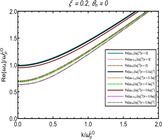
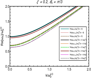
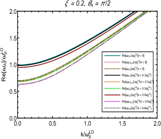
Figure 1: Real A-mode dispersion curve for various EoSs at $\xi=0.2$, $T_{c}=0.17GeV$ and $T=0.25GeV$ at different $\nu$.

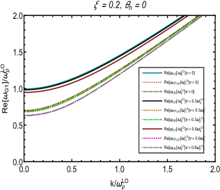
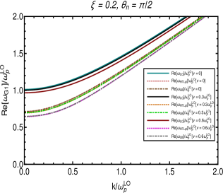
Figure 2: Real G1-mode dispersion curve for various EoSs at $\xi=0.2$, $T_{c}=0.17GeV$ and $T=0.25GeV$ at different $\nu$.

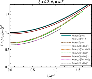
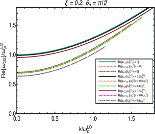
Figure 3: Real G2-mode dispersion curve for various EoSs at $\xi=0.2$, $T_{c}=0.17GeV$ and $T=0.25GeV$ at different $\nu$.

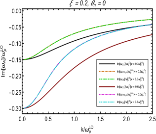
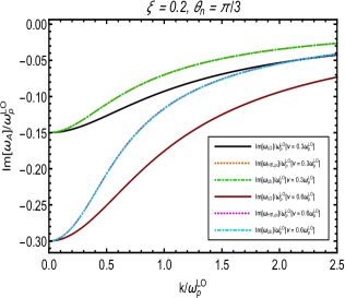
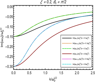
Figure 4: Imaginary A-mode dispersion curves for various EoSs at $\xi=0.2$, $T_{c}=0.17GeV$ and $T=0.25GeV$ at different $\nu$.

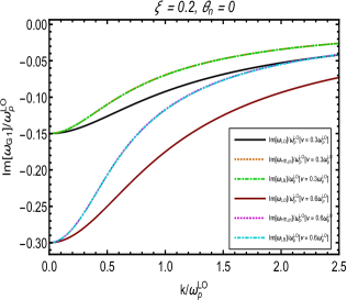
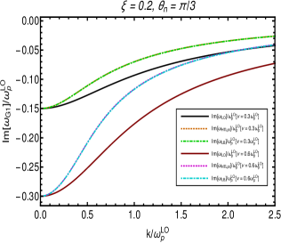
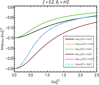
Figure 5: Imaginary G1-mode dispersion curves for various EoSs at $\xi=0.2$, $T_{c}=0.17GeV$ and $T=0.25GeV$ at different $\nu$.

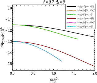
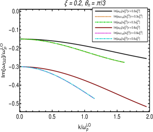
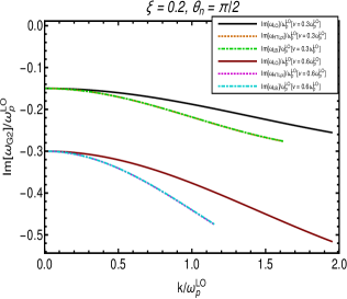
Figure 6: Imaginary G2-mode dispersion curves for various EoSs at $\xi=0.2$, $T_{c}=0.17GeV$ and $T=0.25GeV$ at different $\nu$.

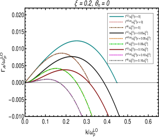
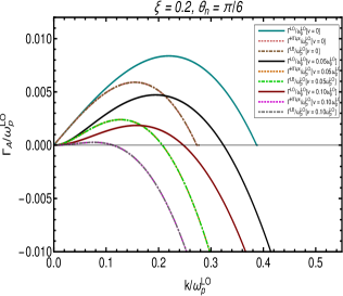
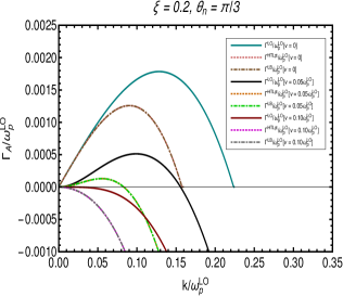
Figure 7: Dispersion curve of unstable A-mode for various EoSs at $\xi=0.2$, $T_{c}=0.17GeV$ and $T=0.25GeV$ with different $\nu$.

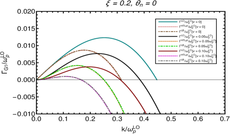
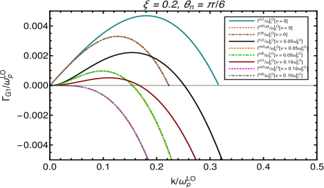
Figure 8: Dispersion curve of G1-mode for various EoSs at $\xi=0.2$, $T_{c}=0.17GeV$ and $T=0.25GeV$ with different $\nu$.

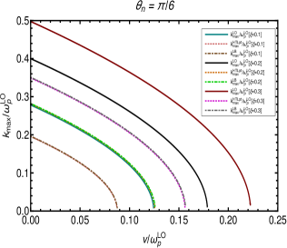
Figure 9: $k_{max}/{\omega^{LO}_{p}}$ vs $\nu/{\omega^{LO}_{p}}$ corresponding to A-mode for various EoSs at $\xi=0.2$, $T_{c}=0.17GeV$ and $T=0.25GeV$ with different $\theta_{n}$.

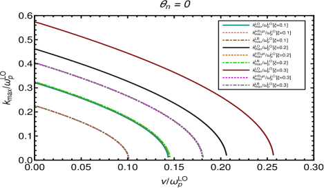
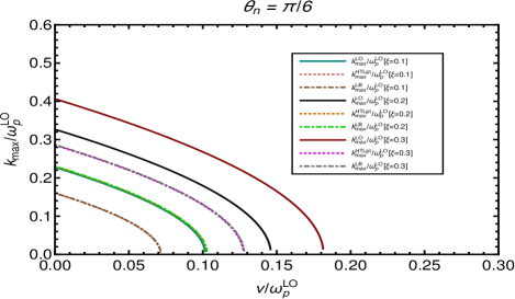
Figure 10: $k_{max}/{\omega^{LO}_{p}}$ vs $\nu/{\omega^{LO}_{p}}$ corresponding to G1-mode for various EoSs at $\xi=0.2$, $T_{c}=0.17GeV$ and $T=0.25GeV$ with different $\theta_{n}$.

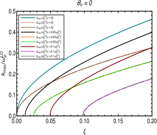
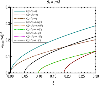
Figure 11: $k_{max}/{\omega^{LO}_{p}}$ vs $\xi$ corresponding to A-mode for various EoSs at $T_{c}=0.17GeV$ and $T=0.25GeV$ with different $\nu$ and $\theta_{n}$.

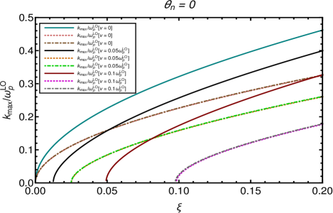
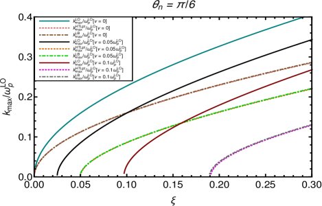
Figure 12: $k_{max}/{\omega^{LO}_{p}}$ vs $\xi$ corresponding to G1-mode for various EoSs at $T_{c}=0.17GeV$ and $T=0.25GeV$ with different $\nu$ and $\theta_{n}$.

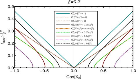
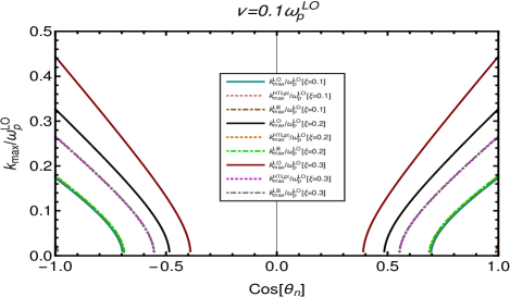
Figure 13: $k_{max}/{\omega^{LO}_{p}}$ vs Cos[$\theta_{n}$] corresponding to A-mode for various EoSs at $\nu=0.1\omega^{LO}_{p}$, $T_{c}=0.17GeV$ and $T=0.25GeV$.

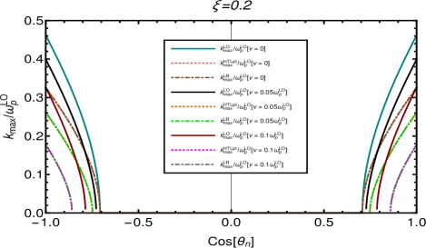
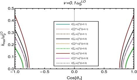
Figure 14: $k_{max}/{\omega^{LO}_{p}}$ vs Cos[$\theta_{n}$] corresponding to G1-mode for various EoSs at $\nu=0.1\omega^{LO}_{p}$, $T_{c}=0.17GeV$ and $T=0.25GeV$.

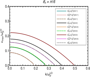
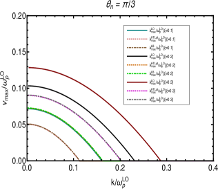
Figure 15: $\nu_{max}/{\omega^{LO}_{p}}$ vs $k/{\omega^{LO}_{p}}$ corresponding to A-mode for various EoSs at $\xi=0.2$, $T_{c}=0.17GeV$, $T=0.25GeV$ with different $\xi$ and $\theta_{n}$.

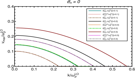
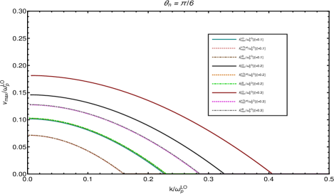
Figure 16: $\nu_{max}/{\omega^{LO}_{p}}$ vs $k/{\omega^{LO}_{p}}$ corresponding to G1-mode for various EoSs at $\xi=0.2$, $T_{c}=0.17GeV$, $T=0.25GeV$ with different $\xi$ and $\theta_{n}$.

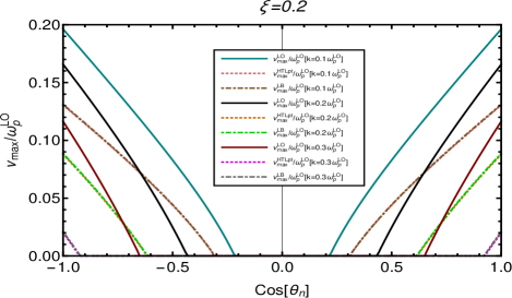
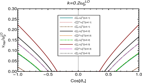
Figure 17: $\nu_{max}/{\omega^{LO}_{p}}$ vs Cos[$\theta_{n}$] corresponding to A-mode for various EoSs at $T_{c}=0.17GeV$ and $T=0.25GeV$.

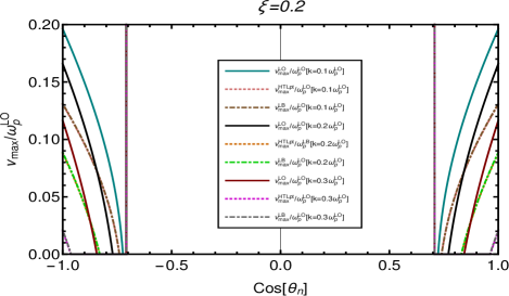
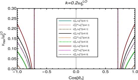
Figure 18: $\nu_{max}/{\omega^{LO}_{p}}$ vs Cos[$\theta_{n}$] corresponding to G1-mode for various EoSs at $T_{c}=0.17GeV$ and $T=0.25GeV$.

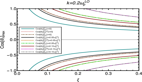
Figure 19: $Cos[\theta_{n}]_{max}$ vs $\xi$ corresponding to A-mode for various EoSs at $\xi=0.2$, $T_{c}=0.17GeV$ and $T=0.25GeV$.

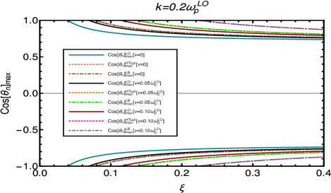
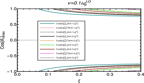
Figure 20: $Cos[\theta_{n}]_{max}$ vs $\xi$ corresponding to G1-mode for various EoSs at $\xi=0.2$, $T_{c}=0.17GeV$ and $T=0.25GeV$.

II.1 Quasi-particle description of Isotropic hot QCD medium

As mentioned earlier, the isotropic/equilibrium state of the QGP has been done within an effective quasi-particle model that describes hot QCD regarding temperature dependent effective fugacity parameters for the gluons and quark/anti-quarks chandra_quasi1 ; chandra_quasi2 . This model is denoted as EQPM (effective fugacity quasi-particle model) here. It is to be noted that there are various quasi-particle models proposed to describe hot QCD medium effects, viz. effective mass models effmass1 ; effmass2 , effective mass models with Polyakov loop polya , NJL and PNJL based effective models pnjl , and the EQPM and recent quasi-particle models based on the Gribov-Zwanziger (GZ) quantization results were leading to non-trivial IR-improved dispersion flor .

These quasi-particle models have shown their utility while studying transport properties of the QGP Bluhm ; chandra_eta ; chandra_etazeta ; PJI ; Mkap ; Mitra:2016zdw . Further, thermal conductivity has also been considered, in addition to the viscosities Mkap , again within the effective mass model along with electrical conductivity parameter for the QGP Greco , within EQPM by Mitra and Chandra Mitra:2016zdw estimated the electrical conductivity and charge diffusion coefficients employing EQPM. The EQPM has also been applied to study heavy-quark transport in isotropic Das:2012ck and anisotropic hot QCD medium  Chandra:2015gma along with quarkonia in hot QCD medium Chandra:2010xg ; Agotiya:2016bqr and dileptons in the QGP medium Chandra:2015rdz ; Chandra:2016dwy . An important point to be noted here is that the above models calculations were not able to correctly reproduce the $\eta$ and $\zeta$ that are phenomenologically extracted from the hydrodynamic simulations of the QGP Ryu ; Denicol1 , consistently agreeing with different experimental observables at RHIC. Earlier, we considered the EQPM description of a (2+1)-flavor lattice QCD EoS cheng (LEoS) . In present work, we have updated the model with the 3-loop HTL perturbative EoS (NNLO HTLpt EoS) that has recently been computed by N. Haque et, al. nhaque ; Andersen:2015eoa and agrees remarkably well with the recent lattice results bazabov2014 ; fodor2014 , and very recent (2+1)-flavor lattice EoS by Bazabov et. al bazabov2014 .

The basic quantities that we need to set-up the linearized transport equation are,

• The quasi-particle distribution functions with EQPM, $f_{eq}\equiv\{f_{g},f_{q}\}$ (describing the strong interaction effects in terms of effective fugacities $z_{g,q}$):

  $$f_{g/q}=\frac{z_{g/q}\exp[-\beta E_{p}]}{\bigg{(}1\mp z_{g/q}\exp[-\beta E_{p}]\bigg{)}},$$ (25)

  where $E_{p}=|{\bf p}|$ for the gluons and $\sqrt{|{\bf p}|^{2}+m_{q}^{2}}$ for the quark degrees of freedom ($m_{q}$ denotes the mass of the quarks). Since the model is valid in the deconfined phase of QCD (beyond $T_{c}$), therefore, the mass of the light quarks can be neglected as compared to the temperature.

• The dispersion relation both in the gluonic and quark sectors:

  $$\omega_{g/q}=E_{p}+T^{2}\partial_{T}ln(z_{g/q}).$$ (26)

• The Debye mass parameter ($m_{D}$) and the effective coupling are other important quantities that are needed in our analysis throughout. Following the definition of $m_{D}$ derived in semi-classical transport theory dmass1 ; dm_rev1 ; dm_rev2 given below in terms of equilibrium gluonic and quark/anti-quark distribution function can be employed here,

  $$m_{D}^{2} = -4\pi\alpha_{s}(T)\bigg{(}2N_{c}\int\frac{d^{3}p}{(2\pi)^{3}}\partial_{p}f_{g}({\bf p})$$ (27)

  $$+ 2N_{f}\int\frac{d^{3}p}{(2\pi)^{3}}\partial_{p}f_{q}({\bf p})\bigg{)},$$

  where, $\alpha_{s}(T)$ is the QCD running coupling constant at finite temperature qcd_coupling . Employing EQPM, we obtain the following expression,

  $${m_{D}^{2}}^{l} = 4\pi\alpha_{s}(T)T^{2}\bigg{(}\frac{2N_{c}}{\pi^{2}}PolyLog[2,z_{g}^{l}]$$ (28)

  $$- \frac{2N_{f}}{\pi^{2}}PolyLog[2,-z_{q}^{l}]\bigg{)}.$$

  where $l$ denotes different EoSs employed here with $z_{g/q}\rightarrow 1$, corresponds to LO or ideal EoS. The effective coupling constant within EQPM that can be read off from the expression for the Debye mass Jamal:2017dqs as,

  $$\alpha_{eff}\equiv\alpha_{s}(T)g(z_{g},z_{q}),$$ (29)

  where,

  $$g(z_{g},z_{q}) = \frac{\frac{2N_{c}}{\pi^{2}}PolyLog[2,z_{g}]-\frac{2N_{f}}{\pi^{2}}PolyLog[2,-z_{q}]}{\frac{N_{c}}{3}+\frac{N_{f}}{6}}.$$

In the next sub-section, we will discuss the calculation of gluon self-energy while incorporating the BGK-colliosional kernel.

II.2 Calculation of gluon self-energy

In order to describe the anisotropic hot QCD medium we follow the arguments of Ref. Romatschke:2003ms where, the anisotropic distribution function was obtained from a isotropic distribution function by rescaling (stretching and squeezing) of one direction in the momentum space as follows.

$$f({\mathbf{p}})\equiv f_{\xi}({\mathbf{p}})=C_{\xi}f(\sqrt{{\bf p}^{2}+\xi({\bf p}\cdot{\bf\hat{n}})^{2}}).$$ (31)

where, ${\mathbf{\hat{n}}}$ is an unit vector (${\bf\hat{n}}^{2}=1$) showing the direction of momentum anisotropy. $C_{\xi}$ is the normalization constant. $\xi$ is the anisotropy parameter which describes the amount of squeezing($\xi>0$) or stretching($-1<\xi<0$) of the distribution function in the ${\bf\hat{n}}$ direction.

Some authors have considered $C_{\xi}$ to be unity  Romatschke:2003ms and later on they normalize anisotropic number density to the isotropic one  Romatschke:2004jh . We want Debye mass to remain undisturbed with the effects of anisotropy so that the effects of various EoSs can be seen clearly. Hence we normalize the Debye mass, also done in Ref. Carrington:2014bla , we get,

$$C_{\xi}=\frac{\sqrt{|\xi|}}{arctan\sqrt{|\xi|}}.$$ (32)

Thus, the Debye mass is not going to get affected by anisotropy but only contains the effects of various EoSs. In small-$\xi$ limit $C_{\xi}$ can be written as,

$$C_{\xi}=1+\frac{\xi}{3}+O({\xi^{2}}).$$ (33)

Now writing down the equation for the self-energy (LABEL:selfenergy) in temporal gauge for anisotropic hot QCD medium with quasi particle description and making a change of variable as ${\mathbf{\tilde{p}}}\equiv\sqrt{{\bf p}^{2}+\xi({\bf p}\cdot{\bf\hat{n}})^{2}}$, we can obtain the following expression,

$$\Pi^{ij}(K) = m_{D}^{2}~{}C_{\xi}\int\frac{d\Omega}{4\pi}v^{i}\frac{v^{l}+\xi(\mathbf{v}\cdot\mathbf{\hat{n}})n^{l}}{(1+\xi(\mathbf{v}\cdot\mathbf{\hat{n}})^{2})^{2}}\left[\delta^{jl}(\omega-\mathbf{k}\cdot\mathbf{v})+v^{j}k^{l}\right]D^{-1}(K,\mathbf{v},\nu)+(i\nu)m_{D}^{2}~{}C_{\xi}\int\frac{d\Omega^{\prime}}{4\pi}(v^{\prime})^{i}$$ (34)

$$\times D^{-1}(K,\mathbf{v}^{\prime},\nu)\int\frac{d\Omega}{4\pi}\frac{v^{l}+\xi(\mathbf{v}\cdot\mathbf{\hat{n}})n^{l}}{(1+\xi(\mathbf{v}\cdot\mathbf{\hat{n}})^{2})^{2}}\big{[}\delta^{jl}(\omega-\mathbf{k}\cdot\mathbf{v})+v^{j}k^{l}\big{]}D^{-1}(K,\mathbf{v},\nu)\mathcal{W}^{-1}(K,\nu),$$

where the Debye mass,

$$m_{D}^{2}=-\frac{g^{2}}{2\pi^{2}}\int_{0}^{\infty}d\tilde{p}\,\tilde{p}^{2}\frac{df_{\text{iso}}(\tilde{p})}{d\tilde{p}}\text{\,.}$$ (35)

is same as given in Eq.(27) and (28). Now as we can see, Eq.(34) is a tensorial equation and hence one can not simply integrate it. We need to construct an analytical form of the gluon self-energy using the available symmetric tensors. In the next sub-section II.2.1, we shall construct $\Pi^{ij}$, analytically and then solve it.

II.2.1 Decomposition of self-energy in terms of structure functions

For isotropic hot QCD plasma we need only the transverse $P^{ij}_{T}=\delta^{ij}-k^{i}k^{j}/{k^{2}}$ and the longitudinal $P^{ij}_{L}=k^{i}k^{j}/{k^{2}}$ tensor projectors to decompose $\Pi^{ij}$. Due to presence of anisotropy vector ${\bf\hat{n}}$, we have to take into account two more projectors $P^{ij}_{n}={\tilde{n}}^{i}{\tilde{n}}^{j}/{\tilde{n}}^{2}$ and $P^{ij}_{kn}=k^{i}{\tilde{n}}^{j}+k^{j}{\tilde{n}}^{i}$ Kobes:1990dc ; Romatschke:2003ms ; Romatschke:2004jh where, $\tilde{n}^{i}=(\delta^{ij}-\frac{k^{i}k^{j}}{k^{2}})\hat{n}^{j}$ is a vector orthogonal to $k^{i}$ i.e. $\mathbf{\tilde{n}}\cdot{\mathbf{k}}=0$. Thus we can decompose the self-energy given in Eq.(LABEL:selfenergy) into following four basis as follows,

$$\Pi^{ij}=\alpha{P}^{ij}_{T}+\beta{P}^{ij}_{L}+\gamma{P}^{ij}_{n}+\delta{P}^{ij}_{kn},$$ (36)

where $\alpha$, $\beta$, $\gamma$ and $\delta$ are some scalar functions which are called structure functions. They can be determined by taking the appropriate projections of the Eq.(LABEL:selfenergy) as follows,

$$\alpha = ({P}^{ij}_{T}-{P}^{ij}_{n})\Pi^{ij},~{}~{}~{}\beta={P}^{ij}_{L}\Pi^{ij},$$

$$\gamma = (2{P}^{ij}_{n}-{P}^{ij}_{T})\Pi^{ij},~{}~{}~{}\delta=\frac{1}{2k^{2}{\tilde{n}}^{2}}{P}^{ij}_{kn}\Pi^{ij}.$$ (37)

The structure functions mainly depend on $k$, $\omega$, $\xi$ $\nu$ and $\mathbf{k\cdot{\hat{n}}}=\cos\theta_{n}$. In the limit $\xi\rightarrow 0$ it can shown that, $\alpha_{\arrowvert_{\xi,\nu=0}}=\Pi_{T}$, $\beta_{\arrowvert_{\xi,\nu=0}}=\frac{\omega^{2}}{k^{2}}\Pi_{L}$, $\gamma_{\arrowvert_{\xi,\nu=0}}=0$, $\delta_{\arrowvert_{\xi,\nu=0}}=0$, where,

$$\Pi_{T} = m^{2}_{D}\frac{\omega^{2}}{2k^{2}}\left[1+\frac{k^{2}-{\omega}^{2}}{2\omega k}\ln\frac{\omega+k}{\omega-k}\right],$$

$$\Pi_{L} = m^{2}_{D}\left[\frac{\omega}{2k}\ln\frac{\omega+k}{\omega-k}-1\right].$$ (38)

Functions $\Pi_{T}$ and $\Pi_{L}$ respectively represent the transverse and longitudinal part of the self-energy for isotropic($\xi=0$) collisionless($\nu=0$)case.

II.2.2 Structure functions in weak anisotropy limit

In the context of heavy ion collisions the anisotropy parameter is defined as, $\xi=\frac{1}{2}\frac{\langle{P^{2}_{T}}\rangle}{\langle{P^{2}_{L}}\rangle}-1$. It is essential to note that the system we are studying is in near-equilibrium, and therefore, we are only considering small values of $\xi$.

In the small anisotropy ($\xi<1$) limit all the structure functions can be calculated analytically. The following expressions for the structure functions can be obtained by expanding the Eq.(LABEL:selfenergy) upto linear order in $\xi$,

$$\alpha\left(\omega,k,\xi,\nu,\theta_{n}\right) = \frac{m_{D}^{2}}{48k}\Bigg{(}24kz^{2}-2k\xi\left(9z^{4}-13z^{2}+4\right)+2i\nu z\left(\xi\left(9z^{2}-7\right)-12\right)-2\xi\cos{2\theta_{n}}\Big{(}k\big{(}15z^{4}-19z^{2}+4\big{)}$$ (39)

$$+i\nu z\big{(}13-15z^{2}\big{)}\Big{)}+\left(z^{2}-1\right)\big{(}3\xi\left(kz\left(5z^{2}-3\right)+i\nu\left(1-5z^{2}\right)\right)\cos{2\theta_{n}}+kz\left(-7\xi+9\xi z^{2}-12\right)$$

$$+i\nu\left(\xi-9\xi z^{2}+12\right)\big{)}\ln\frac{z+1}{z-1}\Bigg{)},$$

$$\beta\left(\omega,k,\xi,\nu,\theta_{n}\right) = -\frac{(2k(kz-i\nu)^{2})\left(m_{D}^{2}\right)}{k^{2}\left(\nu\ln\frac{z+1}{z-1}+2ik\right)}\Bigg{(}1-\frac{1}{2}z\ln\frac{z+1}{z-1}+\frac{1}{12}\xi\left(1+3\cos{2\theta_{n}}\right)\left(2-6z^{2}+\left(3z^{2}-2\right)z\ln{\frac{z+1}{z-1}}\right)\Bigg{)},$$

$$\gamma\left(k,\omega,\xi,\theta_{n},\nu\right)=-\frac{m_{D}^{2}}{12k}{\xi\left(k\left(z^{2}-1\right)-i\nu z\right)\left(4-6z^{2}+3\left(z^{2}-1\right)z\ln\frac{z+1}{z-1}\right)\sin^{2}{\theta_{n}}},$$ (41)

$$\delta\left(\omega,k,\xi,\nu,\theta_{n}\right) = \frac{\xi m_{D}^{2}(kz-i\nu)\cos{\theta_{n}}}{24k^{2}\left(2k-i\nu\ln\frac{z+1}{z-1}\right)}\Bigg{(}k\left(88z-96z^{3}\right)+8i\nu\left(6z^{2}-1\right)+\ln\frac{z+1}{z-1}$$ (42)

$$\times\left(12k\left(4z^{4}-5z^{2}+1\right)-10i\nu z-3~{}i\nu\left(4z^{4}-5z^{2}+1\right)\ln\frac{z+1}{z-1}\right)\Bigg{)},$$

where $z=\frac{\omega+i\nu}{k}$, and

$$\ln\frac{z+1}{z-1}=\ln\frac{|z+1|}{|z-1|}+i\bigg{[}arg\bigg{(}\frac{z+1}{z-1}\bigg{)}+2\pi N\bigg{]}.$$ (43)

Here $N$- corresponds to the number of Riemannian sheets. In the next section, we shall discuss the formalism to find the gluonic collective modes.

III Finding the poles of the propagator (collective modes)

We can also decompose $[\Delta^{-1}(K)]^{ij}$ appearing in Eq.(24) as,

$$[\Delta^{-1}(K)]^{ij} = (k^{2}-{\omega}^{2}+\alpha){P}^{ij}_{T}+(-{\omega}^{2}+\beta){P}^{ij}_{L}$$ (44)

$$+\gamma{P}^{ij}_{n}+\delta{P}^{ij}_{kn}.$$

In order to find out the poles of the propagator $[\Delta(K)]^{ij}$, we first need to know the exact form of $[\Delta(K)]^{ij}$. To achieve that we shall first obtain the inverse of $[\Delta(K)]^{ij}$. We know that if a tensor is exist in a space spanned by some basis vector (projection operators) then its inverse should also exist in the same space, therefore we can also expand $[\Delta(K)]^{ij}$ in the tensor projector basis as of $[\Delta^{-1}(K)]^{ij}$ as follows,

$$[\Delta(K)]^{ij}=a{P}^{ij}_{L}+b{P}^{ij}_{T}+c{P}^{ij}_{n}+d{P}^{ij}_{kn}.$$ (45)

Now, using the relation $[\Delta^{-1}(K)]^{ij}[\Delta(K)]^{jl}=\delta^{il}$ one can obtain the expression for the coefficients $a$, $b$, $c$, $d$ which will yield the following result for the propagator

$$[\Delta(K)]^{ij} = \Delta_{A}({P}^{ij}_{T}-{P}^{ij}_{n})+\Delta_{G}\big{[}(k^{2}-\omega^{2}+\alpha+\gamma){P}^{ij}_{L}$$ (46)

$$+(\beta-\omega^{2}){P}^{ij}_{n}-\delta{P}^{ij}_{kn}\big{]}\,\text{,}$$

with the poles given by

$$\Delta^{-1}_{A}(K) = k^{2}-\omega^{2}+\alpha=0,$$ (47)

$$\Delta^{-1}_{G}(K) = (k^{2}-\omega^{2}+\alpha+\gamma)(\beta-\omega^{2})-k^{2}\tilde{n}^{2}\delta^{2}=0.$$

In the linear $\xi$ approximation we can neglect the term containing $\delta^{2}$ as it will be of order $\xi^{2}$, thus we will have

$$\Delta_{G}^{-1}(K)=(k^{2}-\omega^{2}+\alpha+\gamma)(\beta-\omega^{2})=0.$$ (49)

$\Delta_{G}^{-1}(K)$ can further be written as

$$\Delta_{G}^{-1}(K)=\Delta_{G1}^{-1}(k)~{}\Delta_{G2}^{-1}(k)=0,$$ (50)

Thus, we have two more dispersion equations,

$$\Delta_{G1}^{-1}(K) = k^{2}-\omega^{2}+\alpha+\gamma=0,$$ (51)

$$\Delta_{G2}^{-1}(K) = \beta-\omega^{2}=0.$$ (52)

Note that here we have got three dispersion equations 47, 51 and 52. We call these as A-, G1- and G2-mode dispersion equations respectively. In the next section, we analyze the obtained dispersion equation and present our results. In particular, we explore the instabilities in collisional QGP in small anisotropy($\xi$) and cover the whole range of $\theta_{n}$ (i.e., the angle between the propagation vector($k$) and the direction of anisotropy($\hat{n}$)).

IV Results and Discussions

We solve the dispersion equations (47), (51) and (52) numerically and discuss the results for the stable and unstable modes in the subsections IV.1 and IV.2 respectively. To distinguish the effects of various EoSs (3-loop HTLpt and Lattice Bazabov et. al, 2014) from ideal EoS (LO), we normalize the frequency $\omega$ and wave-number $k$ by $\omega^{LO}_{p}~{}(=m_{D}/\sqrt{3})$ i.e., the leading order plasma frequency.

IV.1 Stable modes

The results for real part of the stable A-, G1-, and G2-modes are shown in Fig.1, 2 and 3, while their imaginary parts are shown in Fig.4, 5 and 6, respectively. These imaginary parts are coming only because of the collisional effects. If we consider the collision-less ($\nu=0$) plasma, these effects vanish. This has been already shown in the studies by different groups Romatschke:2003ms ; Carrington:2014bla ; Jamal:2017dqs . We also did not get the imaginary part of the stable modes for the collision-less case and hence plotted only for non-zero $\nu$.

In Fig.1 we have plotted the real A-modes at fixed anisotropy parameter, $\xi=0.2$ for the cases when $\theta_{n}$ is equal to $0,~{}\pi/3$ and $\pi/2$, respectively. For each case we have shown the variation of Re$({\omega_{A}})/\omega^{Lo}_{p}$ with respect to $k/\omega^{Lo}_{p}$ at different values of $\nu$ for all three EoSs. It can be noticed that for each case (mentioned above), the three curves which starts from the value of Re$({\omega_{A}})/\omega^{Lo}_{p}$ nearly equal to unity corresponds to the ideal EoS where with an increase of the collision frequency ($\nu=0.0,0.3\omega^{Lo}_{p},0.6\omega^{Lo}_{p}$), the modes are marginally suppressed. When one consider the non-ideal EoS the similar pattern repeats but the A-modes get more suppressed due to the non-ideal effect in comparison with the ideal or leading order results. We note here that HTLpt and the lattice EoS results overlap with each other for a given $\nu$ and it is expected.

In a similar way, we have plotted the real parts of stable G1-and G2-modes in Fig-2 and Fig.3, respectively. One can notice by observing Fig-1 and 2, that they do not differ significantly. This can be understood from corresponding dispersions equations (Eq.(47) and (51)). The difference is only because of an additional contribution of the structure constant ($\gamma$) that has negligible effect on the results even for different $\theta_{n}$. This is mainly because of the small dependence of $\xi$. One can also notice from Eq.(41) that the structure constant($\gamma$) vanishes at $\theta_{n}=0$. Hence both the modes overlap which can be clearly seen in Fig. 2 and 3 for $\theta_{n}=0$. We have also got almost similar pattern for the stable G2-mode as shown in Fig.3. However, in case of G2-mode, the behavior is slightly different after a certain value of $k/\omega^{Lo}_{p}$ as the dispersion curve becomes space like (Re$(\omega)<k$).

Fig.4 is plotted for imaginary A-mode for the same values of the parameters $\nu$, $\xi$ and $\theta_{n}$ as discussed in Fig.1. In this case, we did not get the negative imaginary modes for $\nu=0.0$. Thus, we have plotted the dispersion curves only for $\nu=0.3\omega^{Lo}_{p},0.6\omega^{Lo}_{p}$. For the imaginary part of stable A-mode, one can observe from the Fig.4 that as we increase the value of $\nu$, we get Im$[\omega]/\omega^{LO}_{p}$ to be more negative. The non-ideal effects (effect of EoSs) are causing the dispersion curve to be less negative as the $k/\omega^{LO}_{p}$ increases though the curves start from the same point. Here, it can also be noted that the observations at fixed $\xi=0.2$ and different $\theta_{n}$ ($0,~{}\pi/3$ and $\pi/2$) are quite similar. This is due to the fact that negative imaginary modes do not depend on $\xi$ and $\theta$ and is a kind of check of our result that there is no imaginary mode at $\nu=0.0$.

Similarly, we have plotted the imaginary parts of stable G1- and G2-modes in Fig-5 and 6, respectively. For G1-mode we can see that the dispersion curves follow the same pattern as in the case of A-mode. Here also one can notice that results for A- and G1-modes does not seem to differ for the same reason as discussed for the stable G1 mode. For the G2-mode, unlike the case of A- and G1-modes one can see that dispersion curves goes down as we increase $k/\omega^{LO}_{p}$. This is because of the difference in the behavior of the structure functions.

IV.2 Unstable modes

Unstable modes are the positive imaginary solutions of $\omega$ in the dispersion equations (47), (51) and (52). If we substitute $\omega$ to be purely imaginary i.e. $\omega=i\Gamma$, it can be easily seen from Eq.(LABEL:beta) that $\beta>0$. Thus for G2-mode the dispersion equation (Eq.(52)) that transform to $\Gamma^{2}+\beta=0$, will never be satisfied. This is the similar case as shown for collision-less ($\nu=0$) case in earlier studies Romatschke:2003ms ; Carrington:2014bla ; Jamal:2017dqs . Thus out of all three modes there can be only two unstable modes (A and G1). Here we note that G1-mode was not reported in Ref.Schenke:2006xu . This was due to fact that in Ref.Schenke:2006xu only the case $\theta_{n}=0$ was considered (In this situation the structure function $\gamma$ vanishes and A- and G1-modes gets merged). To study unstable A- and G1-modes we have solved the corresponding dispersion equations (Eqs.(47) and (51)) numerically and shown our results in Fig.7 and 8 for the case of weakly squeezed plasma for non-zero collisional rate ($\nu\neq 0$) at different angles($\theta_{n}$).

In Fig.7, we have plotted unstable A-mode at fixed anisotropy, $\xi=0.2$ but different angles ($\theta_{n}=0,\pi/6,\pi/3~{}\text{and}~{}\pi/2$). In order to see the effect of collisions we have taken the different collisional rate ($\nu$) as shown in the figure. In a similar way, we have plotted unstable G1-mode in Fig.8. In both the cases, we find out that with the increase in $\nu$, the unstable modes suppress. The results from both the EoSs are overlapping but suppressing the instability quicker than LO case. For the reason discussed earlier, here also the results of A- and G1-modes are same at $\theta_{n}=0$. As we increase the value of $\theta_{n}$ unstable G1-mode suppresses faster than A-mode. This can be seen from Fig.8 and Fig.7 (see the case $xi=0.2$ and $\theta_{n}=\pi/6$) by comparing the value of $\Gamma_{G1}/\omega^{LO}_{p}$ with that of $\Gamma_{A}/\omega^{LO}_{p}$ at a particular $k/\omega^{LO}_{p}$. The reason is pretty clear here that G1-mode have additional contribution of structure function $\gamma$ which tries to stabilize the modes as we increase $\theta_{n}$ (because of $\sin{\theta_{n}}$ term). However, it is important to note that both the unstable modes decreases as we increase the value of $\theta_{n}$.

As mentioned earlier the unstable modes critically depend on four the parameters $k,\theta_{n},\nu~{}\text{and}~{}\xi$. Therefore, for a given set of any three parameters there must exists a maximum value of fourth parameter (which will be a function of the remaining three) at which instability will completely suppress. In the next subsections IV.2.1,  IV.2.2, and  IV.2.3, we shall discuss the suppression of instability at the maximum value of the parameters $k,~{}\nu~{}\text{and}~{}\theta_{n}$, respectively.

IV.2.1 Maximum values of the k at which instability completely suppresses

The maximum values of $k$ ($k_{max}$) at which instability for modes (A and G1) completely suppressed can be obtained by substituting $\omega=0$ in their dispersion equations. In Fig. 9 we have shown the behavior of $k_{max}$ corresponding to A-mode with respect to $\nu$ scaled with $\omega_{p}^{LO}$ at different $\xi$ ($\xi=0.1,0.2~{}\text{and}~{}0.3$) for $\theta_{n}=0,\pi/6~{}\text{and}~{}\pi/3$. In a similar way the behavior of $k_{max}$ vs $\nu$ scaled with $\omega_{p}^{LO}$ for G1-mode for $\xi=0.1,0.2~{}\text{and}~{}0.3$ at $\theta_{n}=0~{}\text{and}~{}\pi/6$ is shown in Fig.10. In both the cases we have found that with the increase in $\nu$, $k_{max}$ decreases. The same is the case when we increase $\theta_{n}$. Note that unlike for A-mode, we have not shown the plot of $k_{max}$ vs $\nu$ scaled with $\omega_{p}^{LO}$ at $\theta_{n}=\pi/3$. This is due to fact that unstable G1-mode completely suppresses at $\theta_{n}=\pi/3$ irrespective of the value of $k$. One can also note that with the increase in anisotropy, value of $k_{max}$ increases and hence for higher anisotropy, instability can sustain for larger $k$ values. At $\theta_{n}=0$, $k_{max}$ for both the modes is same but at higher value of $\theta_{n}$ ($\theta_{n}=\pi/6$), it suppresses more for G1-mode. To cross check the above facts, we have plotted, respectively, Fig. 11 and 12 for unstable A- and G1-mode for $k_{max}$ with respect to $\xi$ at different values of $\nu$ and got the similar results. Similarly, we have plotted Fig.13 and 14 for $k_{max}$ with respect to $Cos[\theta_{n}]$ for A- and G1-mode, respectively. We can observe that as we move from $\theta_{n}=\pi/2$ to $\theta_{n}=0$ or from $\theta_{n}=\pi/2$ to $\theta_{n}=\pi$, there is symmetry in values of $k_{max}$. This shows that there is a symmetry in the system for the values of $k$, where the instability completely suppress. Also at $\theta_{n}=0~{}\text{and}~{}\pi$, the values of $k_{max}$ for A- and G1- mode are overlapping. This was also expected, as discussed earlier, at $\theta_{n}=0$, $\gamma$ is zero which lead to the same dispersion equations of both the modes. For A-mode, one can also notice that at $\nu=0$, $k_{max}$ is going upto $\theta_{n}=\pm\pi/2$ while for G1-mode it is only going upto $\theta_{n}=\pm\pi/3$. Further more, in all of the above cases we found that the results of other EoSs follows the similar pattern as LO with slightly different numbers.

IV.2.2 Maximum values of the $\nu$ at which instability completely suppresses

In the similar way as we did for $k_{max}$ the value of $\nu_{max}$ can also be obtained at the point where the instabilities completely suppress. In Fig.15 we have shown the behavior of $\nu_{max}/\omega_{p}^{LO}$ for A-mode with respect to $k/\omega_{p}^{LO}$ for different $\xi$ ($\xi=0.1,0.2~{}\text{and}~{}0.3$) at $\theta_{n}=0,\pi/6~{}\text{and}~{}\pi/3$. In a similar way, we have plotted Fig.16 for G1-mode at $\theta_{n}=0~{}\text{and}~{}\pi/6$. Here we have found that with the increase in $k/\omega_{p}^{LO}$, $\nu_{max}/\omega_{p}^{LO}$ decreases and also it gives smaller numbers with the increase in $\theta_{n}$. But with the increase in anisotropy($\xi$), it increases. Again the results for A- and G1-mode are same for $\theta_{n}=0$ but for higher $\theta_{n}$ ($\theta_{n}=\pi/6$), $\nu_{max}$ corresponding to G1-mode decreases faster. In Fig.17 and 18, we have shown the plots of $\nu_{max}$ with respect to $Cos[\theta_{n}]$ for the parameters mentioned in the figures. Here also as we move from $\theta_{n}=\pi/2$ to $\theta_{n}=0$ or from $\theta_{n}=\pi/2$ to $\theta_{n}=\pi$ there is symmetry in values of $\nu_{max}/\omega_{p}^{LO}$ and hence there is a symmetry in the system. Again the EoSs are following the similar pattern with slightly different numbers.

IV.2.3 Maximum values of the $Cos[\theta_{n}]$ or $\theta_{n}$ at which instability completely suppresses

We again follow the similar procedure to obtain maximum values of $Cos[\theta_{n}]$ as we did for $\nu_{max}$ and $k_{max}$. In Fig. 19 and 20, we have plotted maximum possible value of $Cos[\theta_{n}]$ with respect to $\xi$ for A- and G1-modes, respectively with the parameters mentioned in the plots. In both the cases, we have found that as the anisotropy($\xi$) increases, the value of $Cos[\theta_{n}]_{max}$ shifted to the smaller values positive and negative values( or the higher values of $\theta_{n}$ maximum). Thus, we can say that higher the value of $\xi$, higher will be the value of maximum $\theta_{n}$(i.e., towards $\theta_{n}=\pi/2$) or lower will be the value of $Cos[\theta_{n}]_{max}$(i.e., towards $Cos[\theta_{n}]=0$), where the instabilities reach or exist.

V Summary and Conclusions

We have obtained the analytical results for the gluon self-energy in terms of structure functions in the presence of BGK collisional kernel for a hot anisotropic QCD medium in the small anisotropy limit. The dispersion equations for collective modes have been obtained regarding the structure functions of the gluon self-energy. We have studied the stable modes, which are found to have less affected by the anisotropy. We have also investigated the unstable modes and found that the presence of anisotropy and the collision frequency profoundly affects the instabilities of the system. We have incorporated the QCD medium interaction by exploiting the quasi-particle description of the hot QCD equations of state concerning quark and gluon effective fugacities in their distribution functions. The EoSs include 3-loop HTLpt and a very recent Lattice EoS along with ideal EoS.

It turns out that the results obtained for collective modes are very close (irrespective of any change in anisotropy parameter and collision frequency) for first two EoSs and differ significantly in numbers with the case of ideal EoS. This suggests us that the interactions affect the modes significantly (temperature dependence). Hence the instabilities in QGP is found to have a high impact of collisional frequency and anisotropy and also have directionality dependence.

To get a more closer picture to the experiments, one can also observe the behavior of collective mades while subsuming the non-local BGK kernel. This will be taken up in near future.

VI Acknowledgements

VC would like to sincerely acknowledge DST, Govt. of India for Inspire Faculty Award -IFA13/PH-15 and Early Career Research Award(ECRA/2016) Grant. We would like to acknowledge Sukanya Mitra for providing numerical help in effective description of hot QCD equations of state employed in the present work. We further acknowledge Amit Reza, Soumen Roy, Chkresh Singh and Manu George for their help in developing numerical understanding of the work. A. Kumar acknowledges the hospitality of IIT Gandhinagar. We would like to acknowledge people of INDIA for their generous support for the research in fundamental sciences in the country.

References

- (1) J. Adams et al. (STAR Collaboration), Nucl. Phys. A 757, 102 (2005); K. Adcox et al. PHENIX Collaboration, Nucl. Phys. A 757, 184 (2005); B.B. Back et al. PHOBOS Collaboration, Nucl. Phys. A 757, 28 (2005); I. Arsene et al. BRAHMS Collaboration, Nucl. Phys. A 757, 1 (2005).
- (2) K. Aamodt et al. (The Alice Collaboration), Phys. Rev. Lett. 105, 252302 (2010); Phys. Rev. Lett. 105, 252301 (2010); Phys. Rev. Lett. 106, 032301 (2011).
- (3) S. Ryu, J. F. Paquet, C. Shen, G. S. Denicol, B. Schenke, S. Jeon, C. Gale, Phys. Rev. Lett. 115, 132301 (2015).
- (4) G. Denicol, A. Monnai, B. Schenke, Phys. Rev. Lett. 116, 212301 (2016).
- (5) M. C. Chu and T. Matsui, Phys. Rev. D 39, 1892 (1989).
- (6) L.D.Landau and E.M.Lifshitz, Electrodynamics of continuous media, Butterworth-Heinemann, (1984).
- (7) Y. Koike, AIP Conf. Proc. 243, 916 (1992) .
- (8) S. Mrowczynski, Phys. Lett. B 314, 118 (1993).
- (9) S. Mrowczynski, Phys. Rev. C 49, 2191 (1994).
- (10) S. Mrowczynski, Phys. Lett. B 393, 26 (1997).
- (11) M. Y. Jamal, S. Mitra and V. Chandra, Phys. Rev. D 95, 094022 (2017)
- (12) Avdhesh Kumar, Jitesh. R. Bhatt, Predhiman. K. Kaw, Phys. Letts. B 757, 317-323 (2016).
- (13) Daniel F. Litim, C. Manual, Phys. Rep. 364, 451 (2002).
- (14) J.-P.Blaizot and E.Iancu, Phys. Rep. 359, 355 (2002).
- (15) S. Mrowczynski and M. H. Thoma, Phys. Rev. D 62, 036011 (2000) .
- (16) S. Mrowczynski, A. Rebhan and M. Strickland, Phys. Rev. D 70, 025004 (2004).
- (17) Yukinao Akamatsu, Naoki Yamamoto, Phys. Rev. Lett.111, 052002 (2013).
- (18) P. L. Bhatnagar, E. P. Gross, and M. Krook, Phys. Rev. 94, 511 (1954).
- (19) Bing-feng Jiang, De-fu Hou and Jia-rong Li, Phys. Rev. D 94, 074026 (2016).
- (20) Bjoern Schenke, Michael Strickland, Carsten Greiner, Markus H. Thoma, Phys. Rev. D 73, 125004 (2006).
- (21) E. S. Weibel, Phys. Rev. Lett. 2, 83 (1959).
- (22) P. B. Arnold, J. Lenaghan and G. D. Moore, JHEP 0308, 002 (2003).
- (23) S. Mrowczynski, Acta Phys. Polon. B 37, 427 (2006).
- (24) P. Romatschke and M.Strickland, Phys. Rev. D 68, 036004 (2003).
- (25) P. Romatschke and M.Strickland Phys. Rev. D 70, 116006 (2004).
- (26) B. Schenke and M. Strickland, Phys. Rev. D 76, 025023 (2007).
- (27) A. Dumitru, Y. Guo and M. Strickland, Phys. Lett. B 662, 37 (2008).
- (28) M. Martinez and M. Strickland, Phys. Rev. C 78, 034917 (2008).
- (29) M. Attems, A. Rebhan and M. Strickland, Phys. Rev. D 87, no.2, 025010 (2013).
- (30) W. Florkowski, R. Maj, R. Ryblewski and M. Strickland, Phys. Rev. C 87, no.3, 034914 (2013).
- (31) M. Carrington, T. Fugleberg, D. Pickering, and M. Thoma, Can. J. Phys. 82, 671 (2004).
- (32) V. Chandra, R. Kumar, V. Ravishankar, Phys. Rev. C 76, 054909 (2007); [Erratum: Phys. Rev. C 76, 069904 (2007)]; V. Chandra, A. Ranjan, V. Ravishankar, Eur. Phys. J. A 40, 109-117 (2009).
- (33) V. Chandra, V. Ravishankar, Phys. Rev. D 84, 074013 (2011).
- (34) A. Peshier et. al, Phys. Lett. B 337, 235 (1994); Phys.Rev. D 54, 2399 (1996).
- (35) A. Peshier, B. Kämpfer, G. Soff, Phys. Rev. C 61,045203 (2000); Phys. Rev. D 66, 094003 (2002); V. M. Bannur, Phys. Rev. C 75, 044905 (2007); ibid. C 78, 045206 (2008), JHEP 0709, 046 (2007); A. Rebhan, P. Romatschke, Phys. Rev. D 68, 0250022 (2003); M. A. Thaler, R. A. Scheider, W. Weise, Phys. Rev. C 69, 035210 (2004); K. K. Szabo, A. I. Toth, JHEP 0306, 008 (2003).
- (36) M. DÉlia, A. Di Giacomo, E. Meggiolaro, Phys. Lett. B 408, 315 (1997); Phys. Rev. D 67, 114504 (2003); P. Castorina, M. Mannarelli, Phys. Rev. C 75, 054901 (2007); Phys. Lett. B 664, 336 (2007); Paolo Alba et al., Nucl. Phys. A 934, 41-51 (2014).
- (37) A. Dumitru, R. D. Pisarski, Phys. Lett. B 525, 95 (2002); K. Fukushima, Phys. Lett. B 591, 277 (2004); S. K. Ghosh et. al, Phys. Rev. D 73, 114007 (2006); H. Abuki, K. Fukushima, Phys. Lett. B 676, 57 (2006); H. M. Tsai, B. Müller, J. Phys. G 36, 075101 (2009).
- (38) W. Florkowski, R. Ryblewski, Nan Su, K. Tywoniuk, Phys. Rev. C 94 no.4, 044904 (2016) ; Acta Phys. Polon. B 47, 1833 (2016).
- (39) P. Chakraborty, J. I. Kapusta , Phys. Rev. C 83, 014906 (2011).
- (40) M. Albright and J. I. Kapusta, Phys. Rev. C 93, 014903 (2016).
- (41) S. Mitra and V. Chandra, Phys. Rev. D 94, no.3, 034025 (2016).
- (42) V. Chandra, Phys. Rev. D 86 114008 (2012); ibid., D 84, 094025 (2011).
- (43) V. Chandra, V. Ravishankar, Eur. Phys. J. C 64, 63-72 (2009); ibid. C 59, 705-714 (2009).
- (44) M. Bluhm, B. Kampfer and K. Redlich,Phys. Rev. C 84, 025201 (2011).
- (45) A. Puglisi, S. Plumari, V. Greco, Phys. Lett. B 751, 326-330 (2015).
- (46) S. K. Das, V. Chandra and J. e. Alam, J. Phys. G 41, 015102 (2013).
- (47) V. Chandra and S. K. Das, Phys. Rev. D 93, no.9, 094036 (2016).
- (48) V. Chandra and V. Ravishankar, Nucl. Phys. A 848, 330 (2010).
- (49) V. K. Agotiya, V. Chandra, M. Y. Jamal and I. Nilima, Phys. Rev. D 94, no.9, 094006 (2016)
- (50) V. Chandra and V. Sreekanth, Phys. Rev. D 92, no.9, 094027 (2015).
- (51) V. Chandra and V. Sreekanth, arXiv:1602.07142 [nucl-th].
- (52) M. Cheng et. al, Phys. Rev. D 77, 014511 (2008).
- (53) N. Haque, A. Bandyopadhyay, J. O. Andersen, Munshi G. Mustafa, M. Strickland and Nan Su, JHEP 1405, 027 (2014).
- (54) J. O. Andersen, N. Haque, M. G. Mustafa and M. Strickland, Phys. Rev. D 93, no.5, 054045 (2016)
- (55) A. Bazabov et, al., Phys. Rev D 90, 094503 (2014).
- (56) S. Borsanyi, Z. Fodor, C. Hoelbling, S. D. Katz, S. Krieg, Kalman K. Szabo, Phys. Lett. B 370, 99-104, (2014).
- (57) P. F. Kelly et. al, Phys. Rev. Lett. 72, 3461 (1994); Phys. Rev. D 50, 4209 (1995).
- (58) M. Laine and Y. Schöder, JHEP 0503, 067 (2005).
- (59) M. E. Carrington, K. Deja and S. Mrowczynski, Phys. Rev. C 90, no.3, 034913 (2014).
- (60) R. Kobes, G. Kunstatter and A. Rebhan, Nucl. Phys. B 355, 1 (1991).