Error Analysis of Non Inf-sup Stable Discretizations of the time-dependent Navier–Stokes Equations with Local Projection Stabilization

Abstract

This paper studies non inf-sup stable finite element approximations to the evolutionary Navier–Stokes equations. Several local projection stabilization (LPS) methods corresponding to different stabilization terms are analyzed, thereby separately studying the effects of the different stabilization terms. Error estimates are derived in which the constants in the error bounds are independent of inverse powers of the viscosity. For one of the methods, using velocity and pressure finite elements of degree $l$, it will be proved that the velocity error in $L^{\infty}(0,T;L^{2}(\Omega))$ decays with rate $l+1/2$ in the case that $\nu\leq h$, with $\nu$ being the dimensionless viscosity and $h$ the mesh width. In the analysis of another method, it was observed that the convective term can be bounded in an optimal way with the LPS stabilization of the pressure gradient. Numerical studies confirm the analytical results.

1 Introduction

Let $\Omega\subset{\mathbb{R}}^{d}$, $d\in\{2,3\}$, be a bounded domain with polyhedral and Lipschitz boundary $\partial\Omega$. The incompressible Navier–Stokes equations model the conservation of linear momentum and the conservation of mass (continuity equation) by

$$\partial_{t}\boldsymbol{u}-\nu\Delta\boldsymbol{u}+(\boldsymbol{u}\cdot\nabla)\boldsymbol{u}+\nabla p =\boldsymbol{f} \text{in }\ (0,T]\times\Omega,$$

$$\nabla\cdot\boldsymbol{u} =0 \text{in }\ (0,T]\times\Omega,$$ (1)

$$\boldsymbol{u}(0,\cdot) =\boldsymbol{u}_{0}(\cdot) \text{in }\ \Omega,$$

where $\boldsymbol{u}$ is the velocity field, $p$ the kinematic pressure, $\nu>0$ the kinematic viscosity coefficient, $\boldsymbol{u}_{0}$ a given initial velocity, and $\boldsymbol{f}$ represents the external body accelerations acting on the fluid. The Navier–Stokes equations (1) are equipped with homogeneous Dirichlet boundary conditions $\boldsymbol{u}=\boldsymbol{0}$ on $\partial\Omega$.

This paper studies approximations to the Navier–Stokes equations (1) with non inf-sup stable mixed finite elements in space and the implicit Euler method in time. We use the so-called local projection stabilization (LPS) method to stabilize the pressure (since non inf-sup stable elements are used) plus other stabilization terms which aim at allowing to derive error estimates where the constants do not depend explicitly on inverse powers of the viscosity but only implicitly through norms of the solution of (1). This kind of bounds are called semi-robust or quasi-robust in the literature, see for example [4].

In the literature, one can find already investigations of LPS methods for approximating the solution of (1). LPS methods for inf-sup stable elements are analyzed in [3]. The derived error bounds depend explicitly on inverse powers of the viscosity parameter $\nu$, unless the grids are becoming sufficiently fine ($h\lesssim\sqrt{\nu}$, where $h$ is the mesh width), see also [13] where error bounds for the Oberbeck-Boussinesq model model are obtained with an assumption on the regularity of the finite element solution. In [2], the authors consider non inf-sup stable mixed finite elements with LPS stabilization. The so called term-by-term stabilization is applied, see [11]. This method is a particular type of a LPS method that is based on continuous functions, it does not need enriched finite element spaces, and an interpolation operator replaces the standard projection operator of the classical LPS methods. As in the present paper, a fully discrete scheme with the implicit Euler method as time integrator is considered. A fully discrete LPS method for inf-sup stable pairs of finite element spaces and a pressure-projection scheme is analyzed in [4].

Our analysis starts as in [2], but there are several major differences in the formulation of the discrete problem as well as in the obtained results. First of all, as an important result which was not achieved in [2], we are able to derive error bounds in which the constants do not depend on inverse powers of the diffusion parameter. Also, contrary to [2], where only one method is analyzed (with LPS stabilizations of the pressure, the divergence, and the convective term), we consider several methods, because our aim is to study separately the effects of the different stabilization terms. For all of them, error bounds with constants independent on inverse powers of the diffusion parameter are achieved with the smallest possible number of stabilization terms. Also, in contrast to [2], only moderate assumptions on the smallness of the time step $\Delta t$ are needed, like $\Delta t\leq Ch^{d/2}$ in the error analysis of the pressure, while in [2] the smallness assumption on the mesh width $Ch\leq\Delta t$ is required.

Section 3 considers a method with LPS stabilization for the pressure and a global grad-div stabilization term. The global grad-div stabilization term was proposed to reduce the violation of mass conservation of finite element methods, but there are already investigations which show that this term also stabilizes dominant convection. In [14], semi-robust error estimates are proved for the standard Galerkin method plus grad-div stabilization in the case of inf-sup stable elements, both for the continuous-in-time case and for the fully discrete case. Paper [14] considers both, the regular case and the situation in which nonlocal compatibility conditions for the solution are not assumed. The results of Section 3 can be seen as an extension of some of the results from [14] to the case of non inf-sup stable elements and also as an improvement of the results from [2]. Error bounds of order $\mathcal{O}(h^{s})$ are obtained for a sufficiently smooth solution, where $2\leq s\leq l$, $s$ being the regularity index of the solution and $l$ being the degree of the polynomials used. The error is bounded in a norm that includes the $L^{2}$ norm of the velocity at the final time step and the $L^{2}$ norm of the divergence. This rate of convergence is the same as obtained in [14] for a similar norm and also the same rate as proved in [2]. However, as we pointed out above, in [2] more terms are included in the method, the bound depends explicitly on $\nu^{-1}$, and the restriction $Ch\leq\Delta t$ is assumed. For the error bound of the pressure, we get the optimal order $\mathcal{O}(h^{s})$. However, following the ideas of [2], we are able to bound the error of the $L^{2}$ norm of a discrete in time primitive of the pressure instead of the stronger discrete in time $L^{2}$ norm of the pressure. Although Section 3 studies the term-by-term stabilization, the analysis also holds for the standard one-level LPS method, see [15, 21], with slight modifications.

In Section 4, we analyze a method with LPS stabilization for the pressure and LPS stabilization with control of the fluctuations of the gradient. For this section, the use of term-by-term stabilization is necessary since in the error analysis we need to have the same polynomial spaces for the velocity and the pressure. A key ingredient in the error analysis is the application of [8, Theorem 2.2]. This result was already applied in the error analysis in [10], where the authors proved semi-robust error bounds for the evolutionary Navier–Stokes equations and a continuous interior penalty (CIP) method in space assuming enough regularity of the solution. For the method studied in Section 4, the convective term is estimated in an optimal way (with constants independent on inverse powers of the diffusion parameter) with the help of the LPS stabilization of the gradient of the pressure. This LPS term was introduced in [6] to account for the violation of the discrete inf-sup condition by the used pair of finite elements.

Following the analysis of the previous section, Section 5 presents analogous error bounds for a method with both LPS stabilization for the pressure and the divergence.

For the methods analyzed in Sections 3 – 5, error estimates with constants independent on inverse powers of the diffusion parameter are derived with the help of stabilization terms that were not proposed for stabilizing dominant convection but to account for the non-satisfaction of the discrete inf-sup condition or the violation of the mass conservation (note that the LPS term of the velocity gradient of the method from Section 4 was not utilized for estimating the convective term). The deeper reasons for this behavior are not yet understood and their explanation is formulated as an open problem in [19].

In Section 6, it is shown that the rate of decay of the velocity error in the situation $\nu\leq h$ can be improved for the method from Section 4 by choosing different values of the stabilization parameters and increasing the regularity assumption for the pressure. Concretely, a bound of order $\mathcal{O}(h^{s+1/2})$ is proved for an error which contains the $L^{2}$ error of the velocity. This is the same order that was obtained for the CIP method in [10] under the same regularity assumptions. We are not aware of any other paper where this order is proved and it is still an open question whether the optimal expected order $\mathcal{O}(h^{s+1})$ for the $L^{2}$ error of the velocity can be achieved or not, see [19].

Finally, Section 7 presents numerical studies that confirm the analytical results.

2 Preliminaries and notation

Throughout the paper, $W^{s,p}(D)$ will denote the Sobolev space of real-valued functions defined on the domain $D\subset\mathbb{R}^{d}$ with distributional derivatives of order up to $s$ in $L^{p}(D)$. These spaces are endowed with the usual norm denoted by $\|\cdot\|_{W^{s,p}(D)}$. If $s$ is not a positive integer, $W^{s,p}(D)$ is defined by interpolation [1]. In the case $s=0$ it is $W^{0,p}(D)=L^{p}(D)$. As it is standard, $W^{s,p}(D)^{d}$ will be endowed with the product norm and, since no confusion can arise, it will be denoted again by $\|\cdot\|_{W^{s,p}(D)}$. The case $p=2$ will be distinguished by using $H^{s}(D)$ to denote the space $W^{s,2}(D)$. The space $H_{0}^{1}(D)$ is the closure in $H^{1}(D)$ of the set of infinitely differentiable functions with compact support in $D$. For simplicity, $\|\cdot\|_{s}$ (resp. $|\cdot|_{s}$) is used to denote the norm (resp. semi norm) both in $H^{s}(\Omega)$ or $H^{s}(\Omega)^{d}$. The exact meaning will be clear by the context. The inner product of $L^{2}(\Omega)$ or $L^{2}(\Omega)^{d}$ will be denoted by $(\cdot,\cdot)$ and the corresponding norm by $\|\cdot\|_{0}$. For vector-valued functions, the same conventions will be used as before. The norm of the dual space $H^{-1}(\Omega)$ of $H^{1}_{0}(\Omega)$ is denoted by $\|\cdot\|_{-1}$. As usual, $L^{2}(\Omega)$ is always identified with its dual, so one has $H^{1}_{0}(\Omega)\subset L^{2}(\Omega)\subset H^{-1}(\Omega)$ with compact injection. The following Sobolev’s embedding [1] will be used in the analysis: For $1\leq p<d/s$ let $q$ be such that $\frac{1}{q}=\frac{1}{p}-\frac{s}{d}$. There exists a positive constant $C$, independent of $s$, such that

$$\|v\|_{L^{q^{\prime}}(\Omega)}\leq C\|v\|_{W^{s,p}(\Omega)},\qquad\frac{1}{q^{\prime}}\geq\frac{1}{q},\quad v\in W^{s,p}(\Omega).$$ (2)

If $p>d/s$ the above relation is valid for $q^{\prime}=\infty$. A similar embedding inequality holds for vector-valued functions.

Using the function spaces

$$V=H_{0}^{1}(\Omega)^{d},\quad Q=L_{0}^{2}(\Omega)=\left\{q\in L^{2}(\Omega):(q,1)=0\right\},$$

the weak formulation of problem (1) is as follows: Find $(\boldsymbol{u},p)\in V\times Q$ such that for all $(\boldsymbol{v},q)\in V\times Q$,

$$(\partial_{t}\boldsymbol{u},\boldsymbol{v})+\nu(\nabla\boldsymbol{u},\nabla\boldsymbol{v})+((\boldsymbol{u}\cdot\nabla)\boldsymbol{u},\boldsymbol{v})-(\nabla\cdot\boldsymbol{v},p)+(\nabla\cdot\boldsymbol{u},q)=(\boldsymbol{f},\boldsymbol{v}),$$ (3)

and $\boldsymbol{u}(0,\cdot)=\boldsymbol{u}_{0}(\cdot)$.

The Hilbert space

$$H^{\rm div}=\{\boldsymbol{u}\in L^{2}(\Omega)^{d}\ \mid\ L^{2}(\Omega)\ni\nabla\cdot\boldsymbol{u}=0,\,\boldsymbol{u}\cdot\mathbf{n}|_{\partial\Omega}=0\}$$

will be endowed with the inner product of $L^{2}(\Omega)^{d}$ and the space

$$V^{\rm div}=\{\boldsymbol{u}\in V\ \mid\ \nabla\cdot\boldsymbol{u}=0\}$$

with the inner product of $V$.

In the error analysis, the Poincaré–Friedrichs inequality

$$\|\boldsymbol{v}\|_{0}\leq C_{PF}\|\nabla\boldsymbol{v}\|_{0}\quad\forall v\in V$$ (4)

will be used.

3 Local projection stabilization with global grad-div stabilization.

Let $\mathcal{T}_{h}$ be a family of triangulations of $\overline{\Omega}$. Given an integer $l\geq 0$ and a mesh cell $K\in\mathcal{T}_{h}$ we denote by $\mathbb{P}_{l}(K)$ the space of polynomials of degree less or equal to $l$. We consider the following finite element spaces

$$Y_{h}^{l} = \left\{v_{h}\in C^{0}(\overline{\Omega})\mid{v_{h}}_{\mid_{K}}\in{\mathbb{P}}_{l}(K),\quad\forall K\in\mathcal{T}_{h}\right\},\ l\geq 1,$$

$${\boldsymbol{Y}}_{h}^{l} = (Y_{h}^{l})^{d},\quad{\boldsymbol{X}}_{h}={\boldsymbol{Y}}_{h}^{l}\cap(H_{0}^{1})^{d},$$

$$Q_{h} = Y_{h}^{l}\cap L_{0}^{2}.$$

It will be assumed that the family of meshes is quasi-uniform and that the following inverse inequality holds for each $v_{h}\in Y_{h}^{l}$, e.g., see [12, Theorem 3.2.6],

$$\|\boldsymbol{v}_{h}\|_{W^{m,p}(K)}\leq C_{\mathrm{inv}}h_{K}^{n-m-d\left(\frac{1}{q}-\frac{1}{p}\right)}\|\boldsymbol{v}_{h}\|_{W^{n,q}(K)},$$ (5)

where $0\leq n\leq m\leq 1$, $1\leq q\leq p\leq\infty$, and $h_{K}$ is the size (diameter) of the mesh cell $K\in\mathcal{T}_{h}$.

We consider the approximation of (1) with the implicit Euler method in time and a LPS method with grad-div stabilization in space. Given ${\boldsymbol{u}}_{h}^{0}=I_{h}\boldsymbol{u}_{0}$, find $(\boldsymbol{u}_{h}^{n+1},p_{h}^{n+1})\in{\boldsymbol{X}}_{h}\times Q_{h}$ such that

$$\left(\frac{\boldsymbol{u}_{h}^{n+1}-\boldsymbol{u}_{h}^{n}}{\Delta t},\boldsymbol{v}_{h}\right)+\nu(\nabla\boldsymbol{u}_{h}^{n+1},\nabla\boldsymbol{v}_{h})+b(\boldsymbol{u}_{h}^{n+1},\boldsymbol{u}_{h}^{n+1},\boldsymbol{v}_{h})-(p_{h}^{n+1},\nabla\cdot\boldsymbol{v}_{h})$$

$$+S_{h}(\boldsymbol{u}_{h}^{n+1},\boldsymbol{v}_{h}) = ({\boldsymbol{f}}^{n+1},\boldsymbol{v}_{h})\quad\forall\boldsymbol{v}_{h}\in{\boldsymbol{X}}_{h},$$ (6)

$$(\nabla\cdot\boldsymbol{u}_{h}^{n+1},q_{h})+s_{\rm pres}(p_{h}^{n+1},q_{h}) = 0\quad\forall q_{h}\in Q_{h},$$

where

$$S_{h}(\boldsymbol{u},\boldsymbol{v}) = \mu(\nabla\cdot\boldsymbol{u},\nabla\cdot\boldsymbol{v}),$$

$$b(\boldsymbol{u},\boldsymbol{v},\boldsymbol{w}) = (B(\boldsymbol{u},\boldsymbol{v}),\boldsymbol{w})\quad\forall\boldsymbol{u},\boldsymbol{v},\boldsymbol{w}\in H_{0}^{1}(\Omega)^{d},$$

$$B(\boldsymbol{u},\boldsymbol{v}) = (\boldsymbol{u}\cdot\nabla)\boldsymbol{v}+\frac{1}{2}(\nabla\cdot\boldsymbol{u})\boldsymbol{v}\quad\forall\boldsymbol{u},\boldsymbol{v}\in H_{0}^{1}(\Omega)^{d},$$

$$s_{\rm pres}(p_{h}^{n+1},q_{h}) = \sum_{K\in\mathcal{T}_{h}}\tau_{p,K}(\sigma^{*}_{h}(\nabla p_{h}^{n+1}),\sigma^{*}_{h}(\nabla q_{h}))_{K},$$

and $\mu$ and $\tau_{p,K}$ are the grad-div and pressure stabilization parameters, respectively. In addition, $\sigma^{*}_{h}=Id-\sigma_{h}^{l-1}$, where $\sigma_{h}^{j}$ is a locally stable projection or interpolation operator from $L^{2}(\Omega)^{d}$ on ${\boldsymbol{Y}}_{h}^{j}$, that is, there exists a constant $C>0$ such that for any $K\in{\mathcal{T}}_{h}$

$$\|\sigma_{h}^{j}(\boldsymbol{v})\|_{L^{2}(K)}\leq C\|\boldsymbol{v}\|_{L^{2}(\omega_{K})},\quad\forall\boldsymbol{v}\in{L^{2}(\Omega)}^{d},$$ (7)

where $\omega_{K}$ is the union of all mesh cells whose intersection with $K$ is not empty. It will be assumed that the number of mesh cells in each set $\omega_{K}$ is bounded independently of the triangulation and of $K$. From (7), also the $L^{2}$ stability of $\sigma^{*}_{h}$ follows. The operator $\sigma_{h}^{j}$ can be chosen as a Bernardi–Girault [7], Girault–Lions [16], or the Scott–Zhang [22] interpolation operator in the space ${\boldsymbol{Y}}_{h}^{j}$ (for a proof of (7) in the case of the last two operators see [9]). The following bound holds for $\boldsymbol{v}\in H^{s}(\Omega)^{d}$,

$$\|\boldsymbol{v}-\sigma_{h}^{j}(\boldsymbol{v})\|_{L^{2}(K)}\leq Ch_{K}^{s}\|\boldsymbol{v}\|_{H^{s}(\omega_{K})},\quad 1\leq s\leq j+1$$ (8)

from which it can be deduced that

$$\|\boldsymbol{v}-\sigma_{h}^{j}(\boldsymbol{v})\|_{0}\leq Ch^{s}|\boldsymbol{v}|_{s},\quad 1\leq s\leq j+1$$ (9)

see [22, 7, 9]. Bounds (8) and (9) will be applied for $j\in\left\{l-1,l\right\}$.

In the sequel, we will assume that

$$\alpha_{1}h_{K}^{2}\leq\tau_{p,K}\leq\alpha_{2}h_{K}^{2}$$ (10)

for some positive constants $\alpha_{1},\alpha_{2}$ independent of $h$. In addition, the notations

$$(f,g)_{\tau_{p}}=\sum_{K\in{\mathcal{T}}_{h}}\tau_{p,K}(f,g)_{K},\quad\|f\|_{\tau_{p}}=(f,f)_{\tau_{p}}^{1/2}$$ (11)

are used.

The following inf-sup condition holds (see [2, Lemma 4.2]).

Lemma 1

The following inf-sup condition holds

$$\|q_{h}\|_{0}\leq\beta_{0}\left(\sup_{\boldsymbol{v}_{h}\in{\boldsymbol{X}}_{h}}\frac{(\nabla\cdot\boldsymbol{v}_{h},q_{h})}{\|\nabla\boldsymbol{v}_{h}\|_{0}}+\|\sigma_{h}^{*}(\nabla q_{h})\|_{\tau_{p}}\right)\quad\forall q_{h}\in Q_{h}.$$

Along the paper we will use the following discrete Gronwall inequality whose proof can be found in [17].

Lemma 2

Let $k,B,a_{j},b_{j},c_{j},\gamma_{j}$ be nonnegative numbers such that

$$a_{j}+k\sum_{j=0}^{n}b_{j}\leq k\sum_{j=0}^{n}\gamma_{j}a_{j}+k\sum_{j=0}^{n}c_{j}+B,\quad for\quad n\geq 0.$$

Suppose that $k\gamma_{j}<1$, for all j, and set $\sigma_{j}=(1-k\gamma_{j})^{-1}$. Then

$$a_{j}+k\sum_{j=0}^{n}b_{j}\leq\exp\left(k\sum_{j=0}^{n}\sigma_{j}\gamma_{j}\right)\left\{k\sum_{j=0}^{n}c_{j}+B\right\},\quad for\quad n\geq 0.$$

3.1 Error bound for the velocity

Let us denote by $\boldsymbol{u}^{n}=\boldsymbol{u}(\cdot,t_{n})$ and by $p^{n}=p(\cdot,t_{n})$. Following [2], we consider an approximation $\hat{\boldsymbol{u}}_{h}^{n}=R_{h}\boldsymbol{u}^{n}\in{\boldsymbol{X}}_{h}\subset{\boldsymbol{Y}}_{h}^{l}$ satisfying

$$(\boldsymbol{u}^{n}-\hat{\boldsymbol{u}}_{h}^{n},\boldsymbol{v}_{h})=0,\quad\forall\boldsymbol{v}_{h}\in{\boldsymbol{Y}}_{h}^{l-1},\quad n=0,1,\ldots,N.$$ (12)

Let us observe that the above definition for $\hat{\boldsymbol{u}}_{h}$ can be applied for any time $t$ so that we can consider that $\hat{\boldsymbol{u}}_{h}$ is continuous in the $t$ variable. The following bound holds, see [2],

$$\|\boldsymbol{u}^{n}-\hat{\boldsymbol{u}}_{h}^{n}\|_{W^{m,p}}\leq Ch^{s+1-m+d/p-d/2}|\boldsymbol{u}^{n}|_{s+1},\quad n=0,1,\ldots,N,$$ (13)

for $m=0,1$, $p\in[1,\infty]$, $s\geq 1$.

Let $\hat{p}_{h}^{n}=I_{h}p^{n}\in Q_{h}$ with $I_{h}$ being the standard interpolation operator. There exists a constant $C>0$ such that

$$\|p^{n}-\hat{p}_{h}^{n}\|_{W^{m,p}}\leq Ch^{s-m+d/p-d/2}|p^{n}|_{s},\quad n=0,1,\ldots,N,\quad m=0,1,$$ (14)

see [9].

Let us denote

$$\hat{\boldsymbol{e}}_{h}^{n}=\hat{\boldsymbol{u}}_{h}^{n}-\boldsymbol{u}^{n},\quad\boldsymbol{e}_{h}^{n}=\hat{\boldsymbol{u}}_{h}^{n}-\boldsymbol{u}_{h}^{n},\quad\hat{\lambda}_{h}^{n}=\hat{p}_{h}^{n}-p^{n},\quad\lambda_{h}^{n}=\hat{p}_{h}^{n}-p_{h}^{n}.$$ (15)

Subtracting the discrete problem (3) from the continuous problem (3) yields the error equation

$$\left(\frac{\boldsymbol{e}_{h}^{n+1}-\boldsymbol{e}_{h}^{n}}{\Delta t},\boldsymbol{v}_{h}\right)+\nu(\nabla\boldsymbol{e}_{h}^{n+1},\nabla\boldsymbol{v}_{h})+b(\hat{\boldsymbol{u}}_{h}^{n+1},\hat{\boldsymbol{u}}_{h}^{n+1},\boldsymbol{v}_{h})-b(\boldsymbol{u}_{h}^{n+1},\boldsymbol{u}_{h}^{n+1},\boldsymbol{v}_{h})$$

$$-(\lambda_{h}^{n+1},\nabla\cdot\boldsymbol{v}_{h})+(\nabla\cdot\boldsymbol{e}_{h}^{n+1},q_{h})+s_{\rm pres}(\lambda_{h}^{n+1},q_{h})+S_{h}(\boldsymbol{e}_{h}^{n+1},\boldsymbol{v}_{h})$$

$$= ({\boldsymbol{\xi}}_{v_{h}}^{n+1},\boldsymbol{v}_{h})+({\boldsymbol{\xi}}_{q_{h}}^{n+1},q_{h})+\nu(\nabla\hat{\boldsymbol{e}}_{h}^{n+1},\nabla\boldsymbol{v}_{h})+s_{\rm pres}(\hat{p}_{h}^{n+1},q_{h})$$

$$+S_{h}(\hat{\boldsymbol{u}}_{h}^{n+1},\boldsymbol{v}_{h})-(\hat{\lambda}_{h}^{n+1},\nabla\cdot\boldsymbol{v}_{h}),$$

for all $\boldsymbol{v}_{h}\in{\boldsymbol{X}}_{h}$ and $q_{h}\in Q_{h}$. In (3.1), ${\boldsymbol{\xi}}_{v_{h}}^{n+1}$ and ${\boldsymbol{\xi}}_{p_{h}}^{n+1}$ are defined as follows

$${\boldsymbol{\xi}}_{v_{h}}^{n+1} = {\boldsymbol{\xi}}_{v_{h},1}^{n+1}+{\boldsymbol{\xi}}_{v_{h},2}^{n+1},$$ (17)

$$({\boldsymbol{\xi}}_{v_{h},1}^{n+1},\boldsymbol{v}_{h}) = -\left(\partial_{t}\boldsymbol{u}^{n+1}-\frac{\hat{\boldsymbol{u}}_{h}^{n+1}-\hat{\boldsymbol{u}}_{h}^{n}}{\Delta t},\boldsymbol{v}_{h}\right),$$ (18)

$$({\boldsymbol{\xi}}_{v_{h},2}^{n+1},\boldsymbol{v}_{h}) = -b(\boldsymbol{u}^{n+1},\boldsymbol{u}^{n+1},\boldsymbol{v}_{h})+b(\hat{\boldsymbol{u}}_{h}^{n+1},\hat{\boldsymbol{u}}_{h}^{n+1},\boldsymbol{v}_{h}),$$ (19)

$$({\boldsymbol{\xi}}_{q_{h}}^{n+1},q_{h}) = (\nabla\cdot\hat{\boldsymbol{e}}_{h}^{n+1},q_{h}).$$

Remark 1  Note that the error equation (3.1) holds even for $(\boldsymbol{v}_{h},q_{h})=(0,q_{h})$ with $q_{h}\in Y_{h}^{l}$. Let $q_{h}\in Y_{h}^{l}$ and denote by $m(q_{h})$ the mean of $q_{h}$, then (3.1) gives

$$(\nabla\cdot\boldsymbol{e}_{h}^{n+1},q_{h}-m(q_{h}))+s_{\rm pres}(\lambda_{h}^{n+1},q_{h}-m(q_{h}))$$

$$= (\nabla\cdot\hat{\boldsymbol{e}}_{h}^{n+1},q_{h}-m(q_{h}))+s_{\rm pres}(\hat{p}_{h}^{n+1},q_{h}-m(q_{h})).$$

Since the terms $(\nabla\cdot\boldsymbol{e}_{h}^{n+1},m(q_{h}))$, $s_{\rm pres}(\lambda_{h}^{n+1},m(q_{h}))$, $(\nabla\cdot\hat{\boldsymbol{e}}_{h}^{n+1},m(q_{h}))$, and $s_{\rm pres}(\hat{p}_{h}^{n+1},m(q_{h}))$ vanish, it follows that

$$(\nabla\cdot\boldsymbol{e}_{h}^{n+1},q_{h})+s_{\rm pres}(\lambda_{h}^{n+1},q_{h})=(\nabla\cdot\hat{\boldsymbol{e}}_{h}^{n+1},q_{h})+s_{\rm pres}(\hat{p}_{h}^{n+1},q_{h})\quad\forall\ q_{h}\in Y_{h}^{l}.$$

Setting $(\boldsymbol{v}_{h},q_{h})=(\boldsymbol{e}_{h}^{n+1},\lambda_{h}^{n+1})$, rearranging terms, and using the Cauchy–Schwarz inequality and Young’s inequality gives

$$\frac{\|\boldsymbol{e}_{h}^{n+1}\|_{0}^{2}}{2\Delta t}-\frac{\|\boldsymbol{e}_{h}^{n}\|_{0}^{2}}{2\Delta t}+\frac{\|\boldsymbol{e}_{h}^{n+1}-\boldsymbol{e}_{h}^{n}\|_{0}^{2}}{2\Delta t}+\frac{\nu}{2}\|\nabla\boldsymbol{e}_{h}^{n+1}\|_{0}^{2}+\|\sigma_{h}^{*}(\nabla\lambda_{h}^{n+1})\|_{\tau_{p}}^{2}$$

$$+S_{h}(\boldsymbol{e}_{h}^{n+1},\boldsymbol{e}_{h}^{n+1})$$

$$\leq \left|b(\boldsymbol{u}_{h}^{n+1},\boldsymbol{u}_{h}^{n+1},\boldsymbol{e}_{h}^{n+1})-b(\hat{\boldsymbol{u}}_{h}^{n+1},\hat{\boldsymbol{u}}_{h}^{n+1},\boldsymbol{e}_{h}^{n+1})\right|+\frac{\|{\boldsymbol{\xi}}_{v_{h}}^{n+1}\|_{0}^{2}}{2}+\frac{\|\boldsymbol{e}_{h}^{n+1}\|_{0}^{2}}{2}$$

$$+\left|({\boldsymbol{\xi}}_{q_{h}}^{n+1},\lambda_{h}^{n+1})\right|+\frac{\nu}{2}\|\nabla\hat{\boldsymbol{e}}_{h}^{n+1}\|_{0}+\left|s_{\rm pres}(\hat{p}_{h}^{n+1},\lambda_{h}^{n+1})\right|$$

$$+\left|S_{h}(\hat{\boldsymbol{u}}_{h}^{n+1},\boldsymbol{e}_{h}^{n+1})\right|+\left|(\hat{\lambda}_{h}^{n+1},\nabla\cdot\boldsymbol{e}_{h})\right|.$$

Now, the terms on the right-hand sid of (3.1) will be bounded. We start with the last two terms. Applying the Cauchy–Schwarz inequality, Young’s inequality, and (13) yields

$$\left|S_{h}(\hat{\boldsymbol{u}}_{h}^{n+1},\boldsymbol{e}_{h}^{n+1})\right| =\mu\left|(\nabla\cdot\hat{\boldsymbol{u}}_{h}^{n+1},\nabla\cdot\boldsymbol{e}_{h}^{n+1})\right|\leq\frac{\mu}{8}\|\nabla\cdot\boldsymbol{e}_{h}^{n+1}\|_{0}^{2}+2\mu\|\nabla\cdot\hat{\boldsymbol{e}}_{h}^{n+1}\|_{0}^{2}$$

$$\leq\frac{1}{8}S_{h}(\boldsymbol{e}_{h}^{n+1}\,\boldsymbol{e}_{h}^{n+1})+C\mu h^{2s}\|\boldsymbol{u}\|_{L^{\infty}(H^{s+1})}^{2}.$$ (21)

Similarly, we obtain

$$\left|(\hat{\lambda}_{h}^{n+1},\nabla\cdot\boldsymbol{e}_{h})\right|\leq\frac{\mu}{8}\|\nabla\cdot\boldsymbol{e}_{h}^{n+1}\|_{0}^{2}+\frac{2}{\mu}\|\hat{\lambda}_{h}^{n+1}\|_{0}^{2}\leq\frac{1}{8}S_{h}(\boldsymbol{e}_{h}^{n+1},\boldsymbol{e}_{h}^{n+1})+\frac{C}{\mu}h^{2s}\|p\|^{2}_{L^{\infty}(H^{s})},$$ (22)

where in the last inequality (14) was applied. The nonlinear term in (3.1) can be bounded as in [14] using the skew-symmetric property of $b$

$$|b(\boldsymbol{u}_{h}^{n+1},\boldsymbol{u}_{h}^{n+1},\boldsymbol{e}_{h}^{n+1})-b(\hat{\boldsymbol{u}}_{h}^{n+1},\hat{\boldsymbol{u}}_{h}^{n+1},\boldsymbol{e}_{h}^{n+1})|$$ (23)

$$\leq |b(\boldsymbol{e}_{h}^{n+1},\hat{\boldsymbol{u}}_{h}^{n+1},\boldsymbol{e}_{h}^{n+1})|+|b(\boldsymbol{u}_{h}^{n+1},\boldsymbol{e}_{h}^{n+1},\boldsymbol{e}_{h}^{n+1})|$$

$$\leq \|\nabla\hat{\boldsymbol{u}}_{h}^{n+1}\|_{L^{\infty}}\|\boldsymbol{e}_{h}^{n+1}\|_{0}^{2}+\frac{1}{2}\|\nabla\cdot\boldsymbol{e}_{h}^{n+1}\|_{0}\|\hat{\boldsymbol{u}}_{h}^{n+1}\|_{L^{\infty}}\|\boldsymbol{e}_{h}^{n+1}\|_{0}$$

$$\leq \left(\|\nabla\hat{\boldsymbol{u}}_{h}^{n+1}\|_{L^{\infty}}+\frac{\|\hat{\boldsymbol{u}}_{h}^{n+1}\|_{L^{\infty}}^{2}}{4\mu}\right)\|\boldsymbol{e}_{h}^{n+1}\|_{0}^{2}+\frac{\mu}{4}\|\nabla\cdot\boldsymbol{e}_{h}^{n+1}\|_{0}^{2}.$$

For the fourth term on the right-hand side of (3.1), integrating by parts and using (12), (10), and (13) gives

$$|({\boldsymbol{\xi}}_{q_{h}}^{n+1},\lambda_{h}^{n+1})| = |(\hat{\boldsymbol{e}}_{h}^{n+1},\nabla\lambda_{h}^{n+1})|=|(\hat{\boldsymbol{e}}_{h}^{n+1},\sigma_{h}^{*}(\nabla\lambda_{h}^{n+1}))|$$ (24)

$$\leq \sum_{K\in{\mathcal{T}}_{h}}\frac{\|\hat{\boldsymbol{e}}_{h}^{n+1}\|_{L^{2}(K)}^{2}}{\tau_{p,K}}+\frac{1}{4}\|\sigma_{h}^{*}(\nabla\lambda_{h}^{n+1}))\|_{\tau_{p}}^{2}$$

$$\leq Ch^{2s}\|\boldsymbol{u}\|_{L^{\infty}(H^{s+1})}^{2}+\frac{1}{4}\|\sigma_{h}^{*}(\nabla\lambda_{h}^{n+1}))\|_{\tau_{p}}^{2}.$$

For the fifth term, we use (13) to get

$$\frac{\nu}{2}\|\nabla\hat{\boldsymbol{e}}_{h}^{n+1}\|_{0}^{2}\leq C\nu h^{2s}\|\boldsymbol{u}\|_{L^{\infty}(H^{s+1})}^{2}.$$ (25)

To bound the sixth term, the usual inequalities, the definition (11) of $\|\cdot\|_{\tau_{p}}$, (9), and (14) are utilized

$$\left|s_{\rm pres}(\hat{p}_{h}^{n+1},\lambda_{h}^{n+1})\right| \leq \|\sigma^{*}_{h}(\nabla\hat{p}_{h}^{n+1})\|^{2}_{\tau_{p}}+\frac{1}{4}\|\sigma^{*}_{h}(\nabla\lambda_{h}^{n+1})\|_{\tau_{p}}^{2}$$ (26)

$$\leq 2\|\sigma^{*}_{h}(\nabla\hat{\lambda}_{h}^{n+1})\|^{2}_{\tau_{p}}+2\|\sigma^{*}_{h}(\nabla p^{n+1})\|^{2}_{\tau_{p}}+\frac{1}{4}\|\sigma^{*}_{h}(\nabla\lambda_{h}^{n+1})\|_{\tau_{p}}$$

$$\leq Ch^{2}\|\nabla\hat{\lambda}_{h}^{n+1}\|_{0}^{2}+Ch^{2}\|\sigma^{*}_{h}(\nabla p^{n+1})\|_{0}^{2}+\frac{1}{4}\|\sigma^{*}_{h}(\nabla\lambda_{h}^{n+1})\|_{\tau_{p}}$$

$$\leq Ch^{2s}\|p\|_{L^{\infty}(H^{s})}^{2}+\frac{1}{4}\|\sigma^{*}_{h}(\nabla\lambda_{h}^{n+1})\|_{\tau_{p}}.$$

Inserting now (3.1) – (26) in (3.1) yields

$$\|\boldsymbol{e}_{h}^{n+1}\|_{0}^{2}-\|\boldsymbol{e}_{h}^{n}\|_{0}^{2}+\Delta t\nu\|\nabla\boldsymbol{e}_{h}^{n+1}\|_{0}^{2}+\Delta t\|\sigma_{h}^{*}(\nabla\lambda_{h}^{n+1})\|_{\tau_{p}}^{2}+\mu\Delta t\|\nabla\cdot\boldsymbol{e}_{h}^{n+1}\|_{0}^{2}$$

$$\leq \Delta t\left(1+2\|\nabla\hat{\boldsymbol{u}}_{h}^{n+1}\|_{L^{\infty}}+\frac{\|\hat{\boldsymbol{u}}_{h}^{n+1}\|_{L^{\infty}}^{2}}{2\mu}\right)\|\boldsymbol{e}_{h}^{n+1}\|_{0}^{2}+\Delta t\|{\boldsymbol{\xi}}_{v_{h}}^{n+1}\|_{0}^{2}$$

$$+C\Delta th^{2s}\left((1+\nu+\mu)\|\boldsymbol{u}\|_{L^{\infty}(H^{s+1})}^{2}+\left(1+\mu^{-1}\right)\|p\|_{L^{\infty}(H^{s})}^{2}\right),$$

such that summing over the discrete times leads to

$$\|\boldsymbol{e}_{h}^{n}\|_{0}^{2}+\Delta t\nu\sum_{j=1}^{n}\|\nabla\boldsymbol{e}_{h}^{j}\|_{0}^{2}+\Delta t\sum_{j=1}^{n}\|\sigma_{h}^{*}(\nabla\lambda_{h}^{j})\|_{\tau_{p}}^{2}+\Delta t{\mu}\sum_{j=1}^{n}\|\nabla\cdot\boldsymbol{e}_{h}^{j}\|_{0}^{2}$$

$$\leq \|\boldsymbol{e}_{h}^{0}\|_{0}^{2}+\sum_{j=1}^{n}\Delta t\left(1+2\|\nabla\hat{\boldsymbol{u}}_{h}^{j}\|_{L^{\infty}}+\frac{\|\hat{\boldsymbol{u}}_{h}^{j}\|_{L^{\infty}}^{2}}{2\mu}\right)\|\boldsymbol{e}_{h}^{j}\|_{0}^{2}+\Delta t\sum_{j=1}^{n}\|{\boldsymbol{\xi}}_{v_{h}}^{j}\|_{0}^{2}$$

$$+CTh^{2s}\left((1+\nu+\mu)\|\boldsymbol{u}\|_{L^{\infty}(H^{s+1})}^{2}+(1+\mu^{-1})\|p\|_{L^{\infty}(H^{s})}^{2}\right).$$

Let us bound $\|\hat{\boldsymbol{u}}_{h}^{j}\|_{L^{\infty}}$ and $\|\nabla\hat{\boldsymbol{u}}_{h}^{j}\|_{L^{\infty}}$, $1\leq j\leq n$. For the first term, applying (2) and (13) we have

$$\|\hat{\boldsymbol{u}}_{h}^{j}\|_{L^{\infty}} \leq \|\boldsymbol{u}^{j}\|_{L^{\infty}}+\|\boldsymbol{u}^{j}-\hat{\boldsymbol{u}}_{h}^{j}\|_{L^{\infty}}\leq C\|\boldsymbol{u}^{j}\|_{2}+Ch^{2-d/2}\|\boldsymbol{u}^{j}\|_{2}$$ (27)

$$\leq C\|\boldsymbol{u}\|_{L^{\infty}(H^{2})}.$$

Using the same argument for the second term, we reach

$$\|\nabla\hat{\boldsymbol{u}}_{h}^{j}\|_{L^{\infty}} \leq \|\nabla\boldsymbol{u}^{j}\|_{L^{\infty}}+\|\nabla\boldsymbol{u}^{j}-\nabla\hat{\boldsymbol{u}}_{h}^{j}\|_{L^{\infty}}\leq C\|\boldsymbol{u}^{j}\|_{3}+Ch^{2-d/2}\|\boldsymbol{u}^{j}\|_{3}$$ (28)

$$\leq C\|\boldsymbol{u}\|_{L^{\infty}(H^{3})}.$$

From (27) and (28) we deduce

$$1+2\|\nabla\hat{\boldsymbol{u}}_{h}^{j}\|_{L^{\infty}}+\frac{\|\hat{\boldsymbol{u}}_{h}^{j}\|_{L^{\infty}}^{2}}{2\mu}\leq\hat{M}_{u},\quad\hat{M}_{u}=1+C\left(2\|\boldsymbol{u}\|_{L^{\infty}(H^{3})}+\frac{\|\boldsymbol{u}\|_{L^{\infty}(H^{2})}^{2}}{2\mu}\right).$$ (29)

Let us assume

$$\Delta t\hat{M}_{u}\leq\frac{1}{2}.$$ (30)

Applying the Gronwall lemma, Lemma 2, we get

$$\|\boldsymbol{e}_{h}^{n}\|_{0}^{2}+\Delta t\nu\sum_{j=1}^{n}\|\nabla\boldsymbol{e}_{h}^{j}\|_{0}^{2}+\Delta t\sum_{j=1}^{n}\|\sigma_{h}^{*}(\nabla\lambda_{h}^{j})\|_{\tau_{p}}^{2}+\Delta t{\mu}\sum_{j=1}^{n}\|\nabla\cdot\boldsymbol{e}_{h}^{j}\|_{0}^{2}$$

$$\leq e^{2T\hat{M}_{u}}\left(\|\boldsymbol{e}_{h}^{0}\|_{0}^{2}+\Delta t\sum_{j=1}^{n}\|{\boldsymbol{\xi}}_{v_{h}}^{j}\|_{0}^{2}\right)$$

$$+Ce^{2T\hat{M}_{u}}\left(Th^{2s}\left((1+\nu+\mu)\|\boldsymbol{u}\|_{L^{\infty}(H^{s+1})}^{2}+(1+\mu^{-1})\|p\|_{L^{\infty}(H^{s})}^{2}\right)\right).$$

To conclude the bound we are left with the task of getting a bound for the second term on the right-hand-side of (3.1). For the first term in the truncation error we write

$$\partial_{t}\boldsymbol{u}^{j}-\frac{\hat{\boldsymbol{u}}_{h}^{j}-\hat{\boldsymbol{u}}^{j-1}_{h}}{\Delta t} = \left(\partial_{t}\boldsymbol{u}^{j}-\frac{\boldsymbol{u}^{j}-\boldsymbol{u}^{j-1}}{\Delta t}\right)+\left(\frac{\boldsymbol{u}^{j}-\boldsymbol{u}^{j-1}}{\Delta t}-\frac{\hat{\boldsymbol{u}}_{h}^{j}-\hat{\boldsymbol{u}}^{j-1}_{h}}{\Delta t}\right)$$

$$= \frac{1}{\Delta t}\int_{t_{j-1}}^{t_{j}}(t-t_{j-1})\partial_{tt}\boldsymbol{u}(t)~{}dt+\frac{1}{\Delta t}\int_{t_{j-1}}^{t_{j}}\partial_{t}(\boldsymbol{u}-\hat{\boldsymbol{u}}_{h})(t)~{}dt.$$

Applying (13) and the Cauchy-Schwarz inequality, we reach

$$\left\|\partial_{t}\boldsymbol{u}^{j}-\frac{\hat{\boldsymbol{u}}_{h}^{j}-\hat{\boldsymbol{u}}^{j-1}_{h}}{\Delta t}\right\|_{0}^{2}\leq C\Delta t\int_{t_{j-1}}^{t_{j}}\|\partial_{tt}\boldsymbol{u}\|_{0}^{2}~{}dt+\frac{h^{2s}}{\Delta t}\int_{t_{j-1}}^{t_{j}}\|\partial_{t}\boldsymbol{u}(t)\|_{s}^{2}~{}dt.$$ (33)

For the second term in the truncation error (19), we apply [14, Lemma 2] to get

$$\sup_{\boldsymbol{\phi}\in L^{2}(\Omega)^{d},\ \|\boldsymbol{\phi}\|_{0}=1}\left|b(\boldsymbol{u}^{j},\boldsymbol{u}^{j},\boldsymbol{\phi})-b(\hat{\boldsymbol{u}}_{h}^{j},\hat{\boldsymbol{u}}_{h}^{j},\boldsymbol{\phi})\right|$$ (34)

$$\leq C\left(\|\hat{\boldsymbol{u}}_{h}^{j}\|_{L^{\infty}}+\|\nabla\cdot\hat{\boldsymbol{u}}^{j}_{h}\|_{L^{2d/(d-1)}}+\|\boldsymbol{u}^{j}\|_{2}\right)\|\boldsymbol{u}^{j}-\hat{\boldsymbol{u}}_{h}^{j}\|_{1}.$$

To bound $\|\nabla\cdot\hat{\boldsymbol{u}}^{j}_{h}\|_{L^{2d/(d-1)}}$ we use (2) and (13)

$$\|\nabla\cdot\hat{\boldsymbol{u}}^{j}_{h}\|_{L^{2d/(d-1)}} \leq \|\nabla\cdot\hat{\boldsymbol{u}}^{j}\|_{L^{2d/(d-1)}}+\|\nabla\cdot(\hat{\boldsymbol{u}}^{j}_{h}-\boldsymbol{u}^{j})\|_{L^{2d/(d-1)}}$$ (35)

$$\leq C\|\boldsymbol{u}^{j}\|_{2}+Ch^{1/2}\|\boldsymbol{u}^{j}\|_{2}$$

$$\leq C\|\boldsymbol{u}\|_{L^{\infty}(H^{2})}.$$

Inserting (27) and (35) in (34) gives

$$\sup_{\boldsymbol{\phi}\in L^{2},\ \|\boldsymbol{\phi}\|_{0}=1}\left|b(\boldsymbol{u}^{j},\boldsymbol{u}^{j},\boldsymbol{\phi})-b(\hat{\boldsymbol{u}}_{h}^{j},\hat{\boldsymbol{u}}_{h}^{j},\boldsymbol{\phi})\right|\leq C\|\boldsymbol{u}\|_{L^{\infty}(H^{2})}\|\boldsymbol{u}^{j}-\hat{\boldsymbol{u}}_{h}^{j}\|_{1}.$$ (36)

Then from (33), (36), and (13) we get

$$\Delta t\sum_{j=1}^{n}\|{\boldsymbol{\xi}}_{v_{h}}^{j}\|_{0}^{2}\leq CTh^{2s}\left(\|\boldsymbol{u}\|_{L^{\infty}(H^{2})}^{2}\|\boldsymbol{u}\|_{L^{\infty}(H^{s+1})}^{2}+\|\partial_{t}\boldsymbol{u}\|_{L^{\infty}(H^{s})}^{2}\right)+C(\Delta t)^{2}\int_{t_{0}}^{t_{n}}\|\partial_{tt}\boldsymbol{u}\|_{0}^{2}~{}dt.$$

Inserting this inequality in (3.1) and applying the triangle inequality to the splitting of the error (15) finishes the proof of the error estimate for the velocity.

Theorem 1

Let the solution of (3) be sufficiently smooth in space and time, such that all norms appearing in the formulation of this theorem are well defined, and let the time step be sufficiently small such that (30) holds. Then, the following error bound holds for $2\leq s\leq l$:

$$\|\boldsymbol{u}^{n}-\boldsymbol{u}_{h}^{n}\|_{0}^{2}+\Delta t\nu\sum_{j=1}^{n}\|\nabla(\boldsymbol{u}^{j}-\boldsymbol{u}_{h}^{j})\|_{0}^{2}+\Delta t\sum_{j=1}^{n}\|\sigma_{h}^{*}(\nabla(p^{j}-p_{h}^{j}))\|_{\tau_{p}}^{2}$$

$$+\Delta t{\mu}\sum_{j=1}^{n}\|\nabla\cdot\boldsymbol{u}_{h}^{j}\|_{0}^{2}$$

$$\leq Ce^{2T\hat{M}_{u}}\left(\|\boldsymbol{e}_{h}^{0}\|_{0}^{2}+T\hat{K}_{u,p}h^{2s}+(\Delta t)^{2}\int_{t_{0}}^{t_{n}}\|\partial_{tt}\boldsymbol{u}\|_{0}^{2}~{}dt\right),$$

where $\hat{M}_{u}$ is defined in (29) and

$$\hat{K}_{u,p}=\left((1+\|\boldsymbol{u}\|_{L^{\infty}(H^{2})}^{2}+\nu+\mu)\|\boldsymbol{u}\|_{L^{\infty}(H^{s+1})}^{2}+\|\partial_{t}\boldsymbol{u}\|_{L^{\infty}(H^{s})}^{2}+(1+\mu^{-1})\|p\|_{L^{\infty}(H^{s})}^{2}\right).$$

Note that neither $\hat{M}_{u}$ nor $\hat{K}_{u,p}$ depend explicitly on negative powers of $\nu$. The error bound (1) can be summarized in the form

$$\mbox{errors on the left-hand side of \eqref{eq:after_gron_2} }\leq C(\boldsymbol{u},\partial_{t}\boldsymbol{u},\partial_{tt}\boldsymbol{u},p,T,\mu,\mu^{-1})\left(\|\boldsymbol{e}_{h}^{0}\|_{0}+h^{s}+\Delta t\right).$$

3.2 Error bound for the pressure

We will derive now a bound for the error in the pressure. Let us denote

$$\Lambda_{h}^{n}=\Delta t\sum_{j=1}^{n}\lambda_{h}^{j},\quad\hat{\Lambda}_{h}^{n}=\Delta t\sum_{j=1}^{n}\hat{\lambda}_{h}^{j}.$$

Setting $q_{h}=0$ in the error equation (3.1) yields

$$(\Lambda_{h}^{n},\nabla\cdot\boldsymbol{v}_{h}) = (\boldsymbol{e}_{h}^{n}-\boldsymbol{e}_{h}^{0},\boldsymbol{v}_{h})+\Delta t\nu\sum_{j=1}^{n}(\nabla(\boldsymbol{u}^{j}-\boldsymbol{u}_{h}^{j}),\nabla\boldsymbol{v}_{h})$$ (38)

$$+\Delta t\sum_{j=1}^{n}\left(b(\boldsymbol{u}^{j},\boldsymbol{u}^{j},\boldsymbol{v}_{h})-b(\boldsymbol{u}_{h}^{j},\boldsymbol{u}_{h}^{j},\boldsymbol{v}_{h})\right)+\Delta t\mu\sum_{j=1}^{n}(\nabla\cdot(\boldsymbol{u}^{j}-\boldsymbol{u}_{h}^{j}),\nabla\cdot\boldsymbol{v}_{h})$$

$$+(\hat{\Lambda}_{h}^{n},\nabla\cdot\boldsymbol{v}_{h})+\Delta t\sum_{j=1}^{n}\left(\partial_{t}\boldsymbol{u}^{j}-\frac{\hat{\boldsymbol{u}}_{h}^{j}-\hat{\boldsymbol{u}}_{h}^{j-1}}{\Delta t},\boldsymbol{v}_{h}\right).$$

Applying Lemma 1 we obtain

$$\|\Lambda_{h}^{n}\|_{0}\leq\beta_{0}\left(\sup_{\boldsymbol{v}_{h}\in{\boldsymbol{X}}_{h}}\frac{(\Lambda_{h}^{n},\nabla\cdot\boldsymbol{v}_{h})}{\|\nabla\boldsymbol{v}_{h}\|_{0}}+\|\sigma_{h}^{*}(\nabla\Lambda_{h}^{n})\|_{\tau_{p}}\right).$$ (39)

Let us bound the first term on the right-hand side of (39). From (38) we get with the triangle inequality, the Poincaré–Friedrichs inequality (4), and the estimate for the dual pairing

$$\sup_{\boldsymbol{v}_{h}\in{\boldsymbol{X}}_{h}}\frac{(\Lambda_{h}^{n},\nabla\cdot\boldsymbol{v}_{h})}{\|\nabla\boldsymbol{v}_{h}\|_{0}} \leq \|\boldsymbol{e}_{h}^{n}\|_{-1}+\|\boldsymbol{e}_{h}^{0}\|_{-1}+\Delta t\nu\sum_{j=1}^{n}\|\nabla(\boldsymbol{u}^{j}-\boldsymbol{u}_{h}^{j})\|_{0}$$ (40)

$$+\Delta t\sum_{j=1}^{n}\|B(\boldsymbol{u}^{j},\boldsymbol{u}^{j})-B(\boldsymbol{u}_{h}^{j},\boldsymbol{u}_{h}^{j})\|_{-1}+\Delta t\mu\sum_{j=1}^{n}\|\nabla\cdot\boldsymbol{u}_{h}^{j}\|_{0}$$

$$+\Delta t\sum_{j=1}^{n}\|\hat{\lambda}_{h}^{j}\|_{0}+\Delta t\sum_{j=1}^{n}\left\|\partial_{t}\boldsymbol{u}^{j}-\frac{\hat{\boldsymbol{u}}_{h}^{j}-\hat{\boldsymbol{u}}_{h}^{j-1}}{\Delta t}\right\|_{-1}.$$

Note that, since $\|\cdot\|_{-1}\leq C\|\cdot\|_{0}$, the first term on the right-hand side of (40) was already bounded in the derivation of the velocity error bound. To bound the third and fifth term on the right-hand side of (40), we use the fact that for any sequence $\left\{\alpha_{j}\right\}_{j=1}^{\infty}$ of nonnegative real numbers and $n\leq T/\Delta t$ by the Cauchy–Schwarz inequality holds

$$\Delta t\sum_{j=1}^{n}\alpha_{j}\leq T^{1/2}\left(\Delta t\sum_{j=1}^{n}\alpha_{j}^{2}\right)^{1/2}.$$ (41)

With this estimate and the velocity error bound (1), an estimate for the third and fifth term is obtained. Using (41) and (33), the bound of the last term on the right-hand side of (40) follows. For the sixth term, we apply (14) to get

$$\Delta t\sum_{j=1}^{n}\|\hat{\lambda}_{h}^{j}\|_{0}\leq CTh^{s}\|p\|_{L^{\infty}(H^{s})}.$$

We are left with the fourth term on the right-hand side of (40). Arguing as in [14], we obtain

$$\Delta t\sum_{j=1}^{n}\|B(\boldsymbol{u}^{j},\boldsymbol{u}^{j})-B(\boldsymbol{u}_{h}^{j},\boldsymbol{u}_{h}^{j})\|_{-1}$$

$$\leq C\Delta t\sum_{j=1}^{n}\left(\|\boldsymbol{u}_{h}^{j}\|_{L^{\infty}}+\|\nabla\cdot\boldsymbol{u}_{h}^{j}\|_{L^{2d/(d-1)}}+\|\boldsymbol{u}^{j}\|_{2}\right)\|\boldsymbol{u}^{j}-\boldsymbol{u}_{h}^{j}\|_{0}$$

$$+C\Delta t\sum_{j=1}^{n}\|\boldsymbol{u}^{j}\|_{1}\|\nabla\cdot(\boldsymbol{u}^{j}-\boldsymbol{u}_{h}^{j})\|_{0}$$

$$\leq CT\left(\max_{1\leq j\leq n}(\|\boldsymbol{u}_{h}^{j}\|_{L^{\infty}}+\|\boldsymbol{u}^{j}\|_{2}\right)\max_{1\leq j\leq n}\|\boldsymbol{u}^{j}-\boldsymbol{u}_{h}^{j}\|_{0}$$

$$+CT^{1/2}\left(\Delta t\sum_{j=1}^{n}\|\nabla\cdot\boldsymbol{u}_{h}^{j}\|_{L^{2d/(d-1)}}^{2}\right)^{1/2}\max_{1\leq j\leq n}\|\boldsymbol{u}^{j}-\boldsymbol{u}_{h}^{j}\|_{0}$$

$$+CT^{1/2}\|\boldsymbol{u}\|_{L^{\infty}(H^{1})}\left(\Delta t\sum_{j=1}^{n}\|\nabla\cdot(\boldsymbol{u}^{j}-\boldsymbol{u}_{h}^{j})\|_{0}^{2}\right)^{1/2}.$$

To bound the norms involving $\boldsymbol{u}_{h}^{j}$, the inverse inequality (5), the Sobolev embedding (2), and (27) are used to get

$$\|\boldsymbol{u}_{h}^{j}\|_{L^{\infty}} \leq \|\boldsymbol{e}_{h}^{j}\|_{L^{\infty}}+\|\hat{\boldsymbol{u}}_{h}^{j}\|_{L^{\infty}}\leq Ch^{-d/2}\|\boldsymbol{e}_{h}^{j}\|_{0}+\|\hat{\boldsymbol{u}}_{h}^{j}\|_{L^{\infty}}$$ (42)

$$\leq Ch^{-d/2}\|\boldsymbol{e}_{h}^{j}\|_{0}+\|\boldsymbol{u}^{j}-\hat{\boldsymbol{u}}_{h}^{j}\|_{L^{\infty}}+\|\boldsymbol{u}^{j}\|_{L^{\infty}}$$

$$\leq Ch^{-d/2}\|\boldsymbol{e}_{h}^{j}\|_{0}+Ch^{2-d/2}\|\boldsymbol{u}\|_{2}+C\|\boldsymbol{u}\|_{2}$$

$$\leq Ch^{-d/2}\|\boldsymbol{e}_{h}^{j}\|_{0}+C\|\boldsymbol{u}\|_{L^{\infty}(H^{2})}.$$

The term $\|\boldsymbol{e}_{h}^{j}\|_{0}$ was already bounded during the derivation of the velocity error estimate. Applying the inverse estimate (5) gives

$$\left(\Delta t\sum_{j=1}^{n}\|\nabla\cdot\boldsymbol{u}_{h}^{j}\|_{L^{2d/(d-1)}}^{2}\right)^{1/2}\leq Ch^{-1/2}\left(\Delta t\sum_{j=1}^{n}\|\nabla\cdot\boldsymbol{u}_{h}^{j}\|_{0}^{2}\right)^{1/2},$$ (43)

where the term on the right-hand side is already bounded in (1). Using (42), (43) and assuming

$$\|\boldsymbol{e}_{h}^{0}\|_{0}=\mathcal{O}(h^{d/2})\quad\mbox{and}\quad\Delta t\leq Ch^{d/2},$$ (44)

we finally reach

$$\Delta t\sum_{j=1}^{n}\|B(\boldsymbol{u}^{j},\boldsymbol{u}^{j})-B(\boldsymbol{u}_{h}^{j},\boldsymbol{u}_{h}^{j})\|_{-1}$$

$$\leq C(\boldsymbol{u},\partial_{t}\boldsymbol{u},\partial_{tt}\boldsymbol{u},p,T,\mu,\mu^{-1})\left(\max_{1\leq j\leq n}\|\boldsymbol{u}^{j}-\boldsymbol{u}_{h}^{j}\|_{0}+\left(\Delta t\sum_{j=1}^{n}\|\nabla\cdot(\boldsymbol{u}^{j}-\boldsymbol{u}_{h}^{j})\|_{0}^{2}\right)^{1/2}\right).$$

The bound of this term is finished by applying (1).

Inserting the derived inequalities in (40) and going back to (39) yields

$$\|\Lambda_{h}^{n}\|_{0} \leq \beta_{0}C(\boldsymbol{u},\partial_{t}\boldsymbol{u},\partial_{tt}\boldsymbol{u},p,T,\mu,\mu^{-1})\left(\|\boldsymbol{e}_{h}^{0}\|_{0}+h^{s}+\Delta t\right)+\beta_{0}\|\sigma_{h}^{*}(\nabla\Lambda_{h}^{n})\|_{\tau_{p}}.$$

The last term was already bounded in the derivation of the velocity error estimate, since it is by the Cauchy–Schwarz inequality

$$\|\sigma_{h}^{*}(\nabla\Lambda_{h}^{n})\|_{\tau_{p}}^{2} = \left\|\Delta t\sum_{j=1}^{n}\sigma_{h}^{*}(\nabla\lambda_{h}^{j})\right\|_{\tau_{p}}^{2}\leq n(\Delta t)^{2}\sum_{j=1}^{n}\|\sigma_{h}^{*}(\nabla\lambda_{h}^{j})\|_{\tau_{p}}^{2}$$

$$= T\Delta t\sum_{j=1}^{n}\|\sigma_{h}^{*}(\nabla\lambda_{h}^{j})\|_{\tau_{p}}^{2},$$

which is a term on the left-hand side of estimate (3.1). The estimate for the pressure error is obtained by applying finally the triangle inequality to the splitting $p^{j}-p_{h}^{j}=\lambda_{h}^{j}-\hat{\lambda}_{h}^{j}$ and using (14).

Theorem 2

Let the assumption of Theorem 1 and the assumptions (44) be satisfied, then the following error estimate holds

$$\left\|\Delta t\sum_{j=1}^{n}(p^{j}-p_{h}^{j})\right\|_{0}\leq\beta_{0}C(\boldsymbol{u},\partial_{t}\boldsymbol{u},\partial_{tt}\boldsymbol{u},p,T,\mu^{-1})\left(\|\boldsymbol{u}_{0}-\boldsymbol{u}_{h}^{0}\|_{0}+h^{s}+\Delta t\right).$$

4 Local projection stabilization with control of the fluctuation of the gradient

In this part we will concentrate on the LPS method based on the stabilization of the gradient. The stabilization term $S_{h}$ is defined by

$$S_{h}(\boldsymbol{u}_{h},\boldsymbol{v}_{h}):=\sum_{K\in\mathcal{T}_{h}}\tau_{\nu,K}\left(\sigma^{*}_{h}(\nabla\boldsymbol{u}_{h}),\sigma_{h}^{*}(\nabla\boldsymbol{v}_{h})\right)_{K},$$ (45)

where $\tau_{\nu,K}$, $K\in\mathcal{T}_{h}$, are non-negative constants. This kind of LPS method gives additional control on the fluctuation of the gradient. In the sequel we will use the notations

$$(f,g)_{\tau_{\nu}}=\sum_{K\in{\mathcal{T}}_{h}}\tau_{\nu,K}(f,g)_{K}\quad\mbox{and}\quad\|f\|_{\tau_{\nu}}=(f,g)_{\tau_{\nu}}^{1/2}.$$

For the stabilization parameter we will take $\tau_{\nu,K}\sim 1$. The same finite element spaces are used as in Section 3.

Assumption A1

There exits an interpolation operator $i_{h}\ :\ H^{2}(\Omega)\rightarrow Q_{h}$ with the approximation properties

$$\big{\|}q-i_{h}q\big{\|}_{0,K}+h_{K}\big{|}q-i_{h}q\big{|}_{1,K}\leq Ch_{K}^{s+1}\big{\|}q\big{\|}_{s+1,K}\quad\forall\ q\in H^{s+1}\big{(}K\big{)},\,1\leq s\leq l,$$ (46)

for all $K\in\mathcal{T}_{h}$. The pressure interpolation operator $i_{h}$ satisfies the orthogonality condition

$$(q-i_{h}q,r_{h})_{K}=0\quad\forall\ q\in Q\cap H^{2}(\Omega),\ r_{h}\in Y_{h}^{l-1},K\in\mathcal{T}_{h}.$$ (47)

Remark 2  The operator $i_{h}$ is the analog in the pressure space to the approximation used in the previous section to bound the velocity error.

Let us observe that the velocity and pressure spaces ${\boldsymbol{Y}}_{h}$ and $Y_{h}$, respectively, are based on piecewise polynomials of the same degree $l$ and are the same space (apart from the fact that the velocity space has $d$ components). This property is essential for applying the following lemma. This lemma can be deduced from [8, Theorem 2.2].

Lemma 3

Let $\sigma_{h}^{j}\ :\ L^{2}(\Omega)^{d}\to{\boldsymbol{Y}}_{h}^{j}$ be the interpolation operation defined in Section 3 and let $\boldsymbol{u}\in W^{1,\infty}(\Omega)^{d}$ and $\boldsymbol{v}_{h}\in{\boldsymbol{Y}}_{h}^{j}$. Then, it holds

$$\|(I-\sigma_{h}^{j})(\boldsymbol{u}\cdot\boldsymbol{v}_{h})\|_{0} \leq Ch\|\boldsymbol{u}\|_{W^{1,\infty}}\|\boldsymbol{v}_{h}\|_{0},$$

$$\|(I-\sigma_{h}^{j})(\boldsymbol{u}\cdot\boldsymbol{v}_{h})\|_{1} \leq C\|\boldsymbol{u}\|_{W^{1,\infty}}\|\boldsymbol{v}_{h}\|_{0}.$$ (48)

Lemma 3 will be applied for $j\in\left\{l-1,l\right\}$.

Remark 3  Lemma 3 holds true for $\boldsymbol{v}_{h}\in{\boldsymbol{Y}}_{h}^{j}$ with several components or $v_{h}\in Y_{h}^{j}$ with only one component.

Remark 4  In this section, in order to apply Lemma 3, we need that the velocity and pressure spaces are the same. Then, the analysis holds for the LPS method based on the term-by-term stabilization introduced in [11]. On the contrary, the analysis of the previous section also holds for the standard one-level LPS method over triangular or quadrilateral elements [15, 21] with slight modifications.

4.1 Error bound for the velocity

We consider the approximation of (3) with the implicit Euler method in time and a LPS method with LPS stabilization for the gradient of the velocity (45) and for the pressure. Given ${\boldsymbol{u}}_{h}^{0}=I_{h}\boldsymbol{u}_{0}$, find $(\boldsymbol{u}_{h}^{n+1},p_{h}^{n+1})\in({\boldsymbol{X}}_{h},Q_{h})$ such that

$$\left(\frac{\boldsymbol{u}_{h}^{n+1}-\boldsymbol{u}_{h}^{n}}{\Delta t},\boldsymbol{v}_{h}\right)+b(\boldsymbol{u}_{h}^{n+1},\boldsymbol{u}_{h}^{n+1},\boldsymbol{v}_{h})+\nu(\nabla\boldsymbol{u}_{h}^{n+1},\nabla\boldsymbol{v}_{h})-(p_{h}^{n+1},\nabla\cdot\boldsymbol{v}_{h})$$

$$+S_{h}(\boldsymbol{u}_{h}^{n+1},\boldsymbol{v}_{h}) = ({\boldsymbol{f}}^{n+1},\boldsymbol{v}_{h}),\quad\forall\boldsymbol{v}_{h}\in{\boldsymbol{X}}_{h},$$

$$(\nabla\cdot\boldsymbol{u}_{h}^{n+1},q_{h})+s_{\rm pres}(p_{h}^{n+1},q_{h}) = 0,\quad\forall q_{h}\in Q_{h}.$$

In the sequel, we will denote by $\hat{\boldsymbol{u}}_{h}^{n}$ the function defined in Assumption A1 satisfying (12) and by $\hat{p}_{h}^{n}=i_{h}p^{n}$ and we denote

$$\hat{\boldsymbol{e}}_{h}^{n}=\hat{\boldsymbol{u}}_{h}^{n}-\boldsymbol{u}^{n},\quad\boldsymbol{e}_{h}^{n}=\hat{\boldsymbol{u}}_{h}^{n}-\boldsymbol{u}_{h}^{n},\quad\hat{\lambda}_{h}^{n}=\hat{p}_{h}^{n}-p^{n},\quad\lambda_{h}^{n}=\hat{p}_{h}^{n}-p_{h}^{n}.$$

It is easy to see that $(\boldsymbol{e}_{h}^{n},\lambda_{h}^{n})$ satisfies the same equation (3.1) as in Section 3.1 and, consequently, (3.1). In the present analysis, the first term on the right-hand side of (3.1) and the last three ones will be treated differently.

Starting as for deriving (23) yields

$$|b(\boldsymbol{u}_{h}^{n+1},\boldsymbol{u}_{h}^{n+1},\boldsymbol{e}_{h}^{n+1})-b(\hat{\boldsymbol{u}}_{h}^{n+1},\hat{\boldsymbol{u}}_{h}^{n+1},\boldsymbol{e}_{h}^{n+1})|$$ (49)

$$\leq \|\nabla\hat{\boldsymbol{u}}_{h}^{n+1}\|_{L^{\infty}}\|\boldsymbol{e}_{h}^{n+1}\|_{0}^{2}+\frac{1}{2}((\nabla\cdot\boldsymbol{e}_{h}^{n+1})\hat{\boldsymbol{u}}_{h}^{n+1},\boldsymbol{e}_{h}^{n+1}).$$

To bound the second term on the right-hand side of (49), we decompose

$$((\nabla\cdot\boldsymbol{e}_{h}^{n+1})\hat{\boldsymbol{u}}_{h}^{n+1},\boldsymbol{e}_{h}^{n+1})$$ (50)

$$=\left((\nabla\cdot\boldsymbol{e}_{h}^{n+1}),{{\sigma_{h}^{l}}}(\hat{\boldsymbol{u}}_{h}^{n+1}\cdot\boldsymbol{e}_{h}^{n+1})\right)+\left((\nabla\cdot\boldsymbol{e}_{h}^{n+1}),(I-{\sigma_{h}^{l}})(\hat{\boldsymbol{u}}_{h}^{n+1}\cdot\boldsymbol{e}_{h}^{n+1})\right).$$

Using the error equation (3.1) with $(\boldsymbol{v}_{h},q_{h})=\left(\boldsymbol{0},{\sigma_{h}^{l}}(\hat{\boldsymbol{u}}_{h}^{n+1}\cdot\boldsymbol{e}_{h}^{n+1})\right)$ gives for the first term on the right-hand side of (50)

$$\left((\nabla\cdot\boldsymbol{e}_{h}^{n+1}),{\sigma_{h}^{l}}(\hat{\boldsymbol{u}}_{h}^{n+1}\cdot\boldsymbol{e}_{h}^{n+1})\right)$$ (51)

$$= s_{\rm pres}(p_{h}^{n+1},{\sigma_{h}^{l}}(\hat{\boldsymbol{u}}_{h}^{n+1}\cdot\boldsymbol{e}_{h}^{n+1}))+(\nabla\cdot\hat{\boldsymbol{e}}_{h}^{n+1},{\sigma_{h}^{l}}(\hat{\boldsymbol{u}}_{h}^{n+1}\cdot\boldsymbol{e}_{h}^{n+1})).$$

For the first term on the right-hand side in (51), arguing as in (26), we have

$$s_{\rm pres}(p_{h}^{n+1},{\sigma_{h}^{l}}(\hat{\boldsymbol{u}}_{h}^{n+1}\cdot\boldsymbol{e}_{h}^{n+1}))$$

$$\leq Ch^{2s}\|p\|_{L^{\infty}(H^{s})}^{2}+\frac{1}{8}\|\sigma^{*}_{h}(\nabla\lambda_{h}^{n+1})\|_{\tau_{p}}^{2}+Ch^{2}\|\sigma^{*}_{h}(\nabla{\sigma_{h}^{l}}(\hat{\boldsymbol{u}}_{h}^{n+1}\cdot\boldsymbol{e}_{h}^{n+1}))\|_{0}^{2}.$$

For the last term above, applying (46), the inverse estimate (5), and (7), it follows that

$$h^{2}\|\sigma^{*}_{h}(\nabla{\sigma_{h}^{l}}(\hat{\boldsymbol{u}}_{h}^{n+1}\cdot\boldsymbol{e}_{h}^{n+1}))\|_{0}^{2} \leq Ch^{2}\|\nabla{\sigma_{h}^{l}}(\hat{\boldsymbol{u}}_{h}^{n+1}\cdot\boldsymbol{e}_{h}^{n+1})\|_{0}^{2}$$

$$\leq Ch^{2}h^{-2}\|{\sigma_{h}^{l}}(\hat{\boldsymbol{u}}_{h}^{n+1}\cdot\boldsymbol{e}_{h}^{n+1})\|_{0}^{2}$$

$$\leq C\|\hat{\boldsymbol{u}}_{h}^{n+1}\|_{L^{\infty}}^{2}\|\boldsymbol{e}_{h}^{n+1}\|_{0}^{2},$$

so that

$$s_{\rm pres}(p_{h}^{n+1},{\sigma_{h}^{l}}(\hat{\boldsymbol{u}}_{h}^{n+1}\cdot\boldsymbol{e}_{h}^{n+1}))$$ (52)

$$\leq Ch^{2s}\|p\|_{L^{\infty}(H^{s})}^{2}+\frac{1}{8}\|\sigma^{*}_{h}(\nabla\lambda_{h}^{n+1})\|_{\tau_{p}}^{2}+C\|\hat{\boldsymbol{u}}_{h}^{n+1}\|_{L^{\infty}}^{2}\|\boldsymbol{e}_{h}^{n+1}\|_{0}^{2}.$$

To bound the second term on the right-hand side of (51), we get with (13) and (7)

$$(\nabla\cdot\hat{\boldsymbol{e}}_{h}^{n+1},{\sigma_{h}^{l}}(\hat{\boldsymbol{u}}_{h}^{n+1}\cdot\boldsymbol{e}_{h}^{n+1}))\leq Ch^{2s}\|\boldsymbol{u}\|_{L^{\infty}(H^{s+1})}^{2}+C\|\hat{\boldsymbol{u}}_{h}^{n+1}\|_{L^{\infty}}^{2}\|\boldsymbol{e}_{h}^{n+1}\|_{0}^{2}.$$

For the second term on the right-hand side of (50), we apply Lemma 3 and the inverse inequality (5) to obtain

$$\left((\nabla\cdot\boldsymbol{e}_{h}^{n+1}),(I-{\sigma_{h}^{l}})(\hat{u}_{h}^{n+1}\cdot\boldsymbol{e}_{h}^{n+1})\right) \leq Ch\|\nabla\cdot\boldsymbol{e}_{h}^{n+1}\|_{0}\|\hat{\boldsymbol{u}}_{h}^{n+1}\|_{W^{1,\infty}}\|\boldsymbol{e}_{h}^{n+1}\|_{0}$$

$$\leq C\|\hat{\boldsymbol{u}}_{h}^{n+1}\|_{W^{1,\infty}}\|\boldsymbol{e}_{h}^{n+1}\|_{0}^{2}.$$

Collecting all estimates, we reach

$$\left|b(\boldsymbol{u}_{h}^{n+1},\boldsymbol{u}_{h}^{n+1},\boldsymbol{e}_{h}^{n+1})-b(\hat{\boldsymbol{u}}_{h}^{n+1},\hat{\boldsymbol{u}}_{h}^{n+1},\boldsymbol{e}_{h}^{n+1})\right|$$ (53)

$$\leq C\left(\|\nabla\hat{\boldsymbol{u}}_{h}^{n+1}\|_{L^{\infty}}+\|\hat{\boldsymbol{u}}_{h}^{n+1}\|_{L^{\infty}}^{2}\right)\|\boldsymbol{e}_{h}^{n+1}\|_{0}^{2}+Ch^{2s}\left(\|p\|_{L^{\infty}(H^{s})}^{2}+\|\boldsymbol{u}\|_{L^{\infty}(H^{s+1})}^{2}\right)$$

$$+\frac{1}{8}\|\sigma^{*}_{h}(\nabla\lambda_{h}^{n+1})\|_{\tau_{p}}^{2}.$$

Remark 5  We like to emphasize the aspect that the only stabilization that was used to derive the optimal estimate (53) of the convective term (in which the constants do not depend on inverse powers of the diffusion parameter) was the LPS stabilization of the pressure – a stabilization term whose proposal does not possess any connection with dominant convection.

The last three terms on the right-hand side of (3.1) will be bounded next. The term $s_{\rm pres}(\hat{p}_{h}^{n+1},\lambda_{h}^{n+1})$ can be bounded as in (26), using (46) instead of (14), and replacing the factor 1/4 multiplying the last term in (26) by 1/8. Also, arguing similarly to (3.1) we have

$$S_{h}(\hat{\boldsymbol{u}}_{h}^{n+1},\boldsymbol{e}_{h}^{n+1}) = (\sigma^{*}_{h}(\nabla\hat{\boldsymbol{u}}_{h}^{n+1}),\sigma^{*}_{h}(\nabla\boldsymbol{e}_{h}^{n+1}))_{\tau_{\nu}}$$

$$\leq \frac{1}{4}\|\sigma^{*}_{h}(\nabla\boldsymbol{e}_{h}^{n+1})\|_{\tau_{\nu}}^{2}+\|\sigma^{*}_{h}(\nabla\hat{\boldsymbol{u}}_{h}^{n+1})\|_{\tau_{\nu}}^{2}$$

$$= \frac{1}{4}S_{h}(\boldsymbol{e}_{h}^{n+1},\boldsymbol{e}_{h}^{n+1})+\|\sigma^{*}_{h}(\nabla\hat{\boldsymbol{u}}_{h}^{n+1})\|_{\tau_{\nu}}^{2}.$$

Then, applying the $L^{2}$ stability of $\sigma_{h}^{*}$, (9), and (13) yields

$$\|\sigma_{h}^{*}(\nabla\hat{\boldsymbol{u}}_{h}^{n+1})\|_{\tau_{\nu}}^{2} \leq \|\sigma_{h}^{*}\nabla(\hat{\boldsymbol{u}}_{h}^{n+1}-\boldsymbol{u}^{n+1})\|_{\tau_{\nu}}^{2}+\|\sigma_{h}^{*}(\nabla\boldsymbol{u}^{n+1})\|_{\tau_{\nu}}^{2}$$

$$\leq C\|\nabla(\hat{\boldsymbol{u}}_{h}^{n+1}-\boldsymbol{u}^{n+1})\|_{0}^{2}+Ch^{2s}\|\boldsymbol{u}\|_{L^{\infty}(H^{s+1})}^{2}$$

$$\leq Ch^{2s}\|\boldsymbol{u}\|_{L^{\infty}(H^{s+1})}^{2},$$

so that

$$S_{h}(\hat{\boldsymbol{u}}_{h}^{n+1},\boldsymbol{e}_{h}^{n+1})\leq\frac{1}{4}S_{h}(\boldsymbol{e}_{h}^{n+1},\boldsymbol{e}_{h}^{n+1})+Ch^{2s}\|\boldsymbol{u}\|_{L^{\infty}(H^{s+1})}^{2}.$$ (54)

Finally, to bound the last term on the right-hand of (3.1), we use the orthogonality condition of the pressure interpolation operator (47), that the norm of the gradient contains all terms of the norm of the divergence and $\|\sigma_{h}^{*}(\nabla\cdot\boldsymbol{e}_{h}^{n+1})\|_{\tau_{\nu}}\leq\sqrt{d}\|\sigma_{h}^{*}(\nabla\boldsymbol{e}_{h}^{n+1})\|_{\tau_{\nu}}$ holds, that $\tau_{\nu,K}\sim 1$, and (46) to get

$$(\hat{\lambda}_{h}^{n+1},\nabla\cdot\boldsymbol{e}_{h}^{n+1}) = -(p^{n+1}-i_{h}p^{n+1},\nabla\cdot\boldsymbol{e}_{h}^{n+1})=-(p^{n+1}-i_{h}p^{n+1},\sigma_{h}^{*}(\nabla\cdot\boldsymbol{e}_{h}^{n+1}))$$ (55)

$$\leq \|p^{n+1}-i_{h}p^{n+1}\|_{\tau_{\nu}^{-1}}\|\sigma_{h}^{*}(\nabla\cdot\boldsymbol{e}_{h}^{n+1})\|_{\tau_{\nu}}$$

$$\leq C\|p^{n+1}-i_{h}p^{n+1}\|_{\tau_{\nu}^{-1}}\|\sigma_{h}^{*}(\nabla\boldsymbol{e}_{h}^{n+1})\|_{\tau_{\nu}}$$

$$\leq C\|p^{n+1}-i_{h}p^{n+1}\|_{0}^{2}+\frac{1}{4}\|\sigma_{h}^{*}(\nabla\boldsymbol{e}_{h}^{n+1})\|_{\tau_{\nu}}^{2}$$

$$\leq Ch^{2s}\|p\|_{L^{\infty}(H^{s})}^{2}+\frac{1}{4}S_{h}(\boldsymbol{e}_{h}^{n+1},\boldsymbol{e}_{h}^{n+1}).$$

Collecting all the estimates we reach

$$\|\boldsymbol{e}_{h}^{n+1}\|_{0}^{2}-\|\boldsymbol{e}_{h}^{n}\|_{0}^{2}+\Delta t\nu\|\nabla\boldsymbol{e}_{h}^{n+1}\|_{0}^{2}+\Delta t\|\sigma_{h}^{*}(\nabla\lambda_{h}^{n+1})\|_{\tau_{p}}^{2}+\|\sigma_{h}^{*}(\nabla\boldsymbol{e}_{h}^{n+1})\|_{\tau_{\nu}}^{2}$$

$$\leq C\Delta t\left(1+\|\nabla\hat{\boldsymbol{u}}_{h}^{n+1}\|_{L^{\infty}}+{\|\hat{\boldsymbol{u}}_{h}^{n+1}\|_{L^{\infty}}^{2}}\right)\|\boldsymbol{e}_{h}^{n+1}\|_{0}^{2}+\Delta t\|{\boldsymbol{\xi}}_{v_{h}}^{n+1}\|_{0}^{2}$$

$$+C\Delta th^{2s}\left((1+\nu)\|\boldsymbol{u}\|_{L^{\infty}(H^{s+1})}^{2}+\|p\|_{L^{\infty}(H^{s})}^{2}\right).$$

From (27) and (28) we deduce

$$1+\|\nabla\hat{\boldsymbol{u}}_{h}^{j}\|_{L^{\infty}}+\|\hat{\boldsymbol{u}}_{h}^{j}\|_{L^{\infty}}^{2}\leq\tilde{M}_{u},\quad\tilde{M}_{u}=1+C\bigl{(}\|\boldsymbol{u}\|_{L^{\infty}(H^{3})}+\|\boldsymbol{u}\|_{L^{\infty}(H^{2})}^{2}\bigr{)}.$$ (56)

Summing up the terms, assuming that

$$\Delta t\tilde{M}_{u}\leq\frac{1}{2},$$ (57)

and applying Lemma 2 (Gronwall) leads to

$$\|\boldsymbol{e}_{h}^{n}\|_{0}^{2}+\Delta t\nu\sum_{j=1}^{n}\|\nabla\boldsymbol{e}_{h}^{j}\|_{0}^{2}+\Delta t\sum_{j=1}^{n}\|\sigma_{h}^{*}(\nabla\lambda_{h}^{j})\|_{\tau_{p}}^{2}+\Delta t\sum_{j=1}^{n}\|\sigma_{h}^{*}(\nabla\boldsymbol{e}_{h}^{j})\|_{\tau_{\nu}}^{2}$$

$$\leq e^{2T\tilde{M}_{u}}\left(\|\boldsymbol{e}_{h}^{0}\|_{0}^{2}+\Delta t\sum_{j=1}^{n}\|{\boldsymbol{\xi}}_{v_{h}}^{j}\|_{0}^{2}+CTh^{2s}\left((1+\nu)\|\boldsymbol{u}\|_{L^{\infty}(H^{s+1})}^{2}+\|p\|_{L^{\infty}(H^{s})}^{2}\right)\right).$$

Now, we can argue exactly as in Section 3.1 to conclude

$$\|\boldsymbol{e}_{h}^{n}\|_{0}^{2}+\Delta t\nu\sum_{j=1}^{n}\|\nabla\boldsymbol{e}_{h}^{j}\|_{0}^{2}+\Delta t\sum_{j=1}^{n}\|\sigma_{h}^{*}(\nabla\lambda_{h}^{j})\|_{\tau_{p}}^{2}+\Delta t\sum_{j=1}^{n}\|\sigma_{h}^{*}(\nabla\boldsymbol{e}_{h}^{j})\|_{\tau_{\nu}}^{2}$$ (59)

$$\leq e^{2T\tilde{M}_{u}}\left(\|\boldsymbol{e}_{h}^{0}\|_{0}^{2}+CT\tilde{K}_{u,p}h^{2s}+C(\Delta t)^{2}\int_{t_{0}}^{t_{n}}\|\partial_{tt}\boldsymbol{u}\|_{0}^{2}\right),$$

with

$$\tilde{K}_{u,p}=\left((1+\|\boldsymbol{u}\|_{L^{\infty}(H^{2})}^{2}+\nu)\|\boldsymbol{u}\|_{L^{\infty}(H^{s+1})}^{2}+\|\partial_{t}\boldsymbol{u}\|_{L^{\infty}(H^{s})}^{2}+\|p\|_{L^{\infty}(H^{s})}^{2}\right).$$ (60)

The triangle inequality finishes the proof of the velocity error estimate.

Theorem 3

Let the solution of (3) be sufficiently smooth in space and time, let the time step be sufficiently small such that (57) holds, and let Assumption A1 be satisfied. Then, the following error bound holds for $2\leq s\leq l$

$$\|\boldsymbol{u}^{n}-\boldsymbol{u}_{h}^{n}\|_{0}^{2}+\Delta t\nu\sum_{j=1}^{n}\|\nabla(\boldsymbol{u}^{j}-\boldsymbol{u}_{h}^{j})\|_{0}^{2}+\Delta t\sum_{j=1}^{n}\|\sigma_{h}^{*}(\nabla(p^{j}-p_{h}^{j}))\|_{\tau_{p}}^{2}$$

$$+\Delta t\sum_{j=1}^{n}\|\sigma_{h}^{*}(\nabla(\boldsymbol{u}^{j}-\boldsymbol{u}_{h}^{j}))\|_{\tau_{\nu}}^{2}$$

$$\leq Ce^{2T\tilde{M}_{u}}\left(\|\boldsymbol{e}_{h}^{0}\|_{0}^{2}+T\tilde{K}_{u,p}h^{2s}+(\Delta t)^{2}\int_{t_{0}}^{t_{n}}\|\partial_{tt}\boldsymbol{u}\|_{0}^{2}~{}dt\right),$$

where the constants on the right-hand side are defined in (56) and (60).

4.2 Error bound for the pressure

The bound for the pressure follows the lines of Section 3.2 with the exception of the bound of the nonlinear term that can be handled as follows

$$\|B(\boldsymbol{u}^{n},\boldsymbol{u}^{n})-B(\boldsymbol{u}_{h}^{n},\boldsymbol{u}_{h}^{n})\|_{-1}\leq\sup_{\|\phi\|_{1}=1}|b(\boldsymbol{u}^{n},\boldsymbol{u}^{n}-\boldsymbol{u}_{h}^{n},\phi)|+\sup_{\|\phi\|_{1}=1}|b(\boldsymbol{u}^{n}-\boldsymbol{u}_{h}^{n},\boldsymbol{u}_{h}^{n},\phi)|.$$

Arguing as before and recalling that $\nabla\cdot\boldsymbol{u}=0$, we can prove

$$\|B(\boldsymbol{u}^{n},\boldsymbol{u}^{n})-B(\boldsymbol{u}_{h}^{n},\boldsymbol{u}_{h}^{n})\|_{-1}\leq\left(\|\boldsymbol{u}^{n}\|_{L^{\infty}}+\|\boldsymbol{u}_{h}^{n}\|_{L^{\infty}}\right)\|\boldsymbol{u}^{n}-\boldsymbol{u}_{h}^{n}\|_{0}+\sup_{\|\phi\|_{1}=1}|((\nabla\cdot\boldsymbol{u}_{h}^{n})\phi,\boldsymbol{u}_{h}^{n})|.$$

The last term can be decomposed as follows

$$((\nabla\cdot\boldsymbol{u}_{h}^{n})\phi,\boldsymbol{u}_{h}^{n})=(\nabla\cdot\boldsymbol{u}_{h}^{n},{\sigma_{h}^{l}}(\phi\cdot\boldsymbol{u}_{h}^{n}))+(\nabla\cdot\boldsymbol{u}_{h}^{n},(I-{\sigma_{h}^{l}})(\phi\cdot\boldsymbol{u}_{h}^{n})).$$ (62)

Since ${\sigma_{h}^{l}}(\phi\cdot\boldsymbol{u}_{h}^{n}))\in{\boldsymbol{Y}}_{h}^{l}$, one can use the error equation (3.1) for estimating the first term in (62). Applying in addition the definition (11) of $\|\cdot\|_{\tau_{p}}$, the choice (10) of the stabilization parameter, the stability (7) of the projection, and the inverse inequality (5) yields

$$(\nabla\cdot\boldsymbol{u}_{h}^{n},{\sigma_{h}^{l}}(\phi\cdot\boldsymbol{u}_{h}^{n})) \leq |s_{\rm pres}(\lambda_{h}^{n},{\sigma_{h}^{l}}(\phi\cdot\boldsymbol{u}_{h}^{n}))|+|s_{\rm pres}(\hat{p}_{h}^{n},{\sigma_{h}^{l}}(\phi\cdot\boldsymbol{u}_{h}^{n}))|$$

$$\leq Ch\left(\|\sigma^{*}_{h}(\nabla\lambda_{h}^{n})\|_{\tau_{p}}+\|\sigma^{*}_{h}(\nabla\hat{p}_{h}^{n})\|_{\tau_{p}}\right)\|\sigma^{*}_{h}(\nabla{\sigma_{h}^{l}}(\phi\cdot\boldsymbol{u}_{h}^{n}))\|_{0}$$

$$\leq C\left(\|\sigma^{*}_{h}(\nabla\lambda_{h}^{n})\|_{\tau_{p}}+\|\sigma^{*}_{h}(\nabla\hat{p}_{h}^{n})\|_{\tau_{p}}\right)\|\phi\cdot\boldsymbol{u}_{h}^{n}\|_{0}.$$

Applying Hölder’s and Sobolev’s inequality, we have

$$\|\phi\cdot\boldsymbol{u}_{h}^{n}\|_{0}\leq\|\phi\|_{L^{2d}}\|\boldsymbol{u}_{h}^{n}\|_{L^{2d/(d-1)}}\leq C\|\phi\|_{1}\|\boldsymbol{u}_{h}^{n}\|_{L^{2d/(d-1)}},$$

so that

$$\sup_{\|\phi\|_{1}=1}(\nabla\cdot\boldsymbol{u}_{h}^{n},{\sigma_{h}^{l}}(\phi\cdot\boldsymbol{u}_{h}^{n}))\leq C\|\boldsymbol{u}_{h}^{n}\|_{L^{2d/(d-1)}}\left(\|\sigma^{*}_{h}(\nabla\lambda_{h}^{n})\|_{\tau_{p}}+Ch^{s}\|p\|_{L^{\infty}(H^{s})}\right).$$

With the decomposition

$$\boldsymbol{u}_{h}^{n}-\boldsymbol{u}^{n}=\boldsymbol{e}_{h}^{n}+\hat{\boldsymbol{u}}_{h}^{n}-\boldsymbol{u}^{n},$$ (64)

the inverse estimate (5), (13), and (9), one obtains for the second term on the right-hand side of (62)

$$(\nabla\cdot\boldsymbol{u}_{h}^{n},(I-{\sigma_{h}^{l}})(\phi\cdot\boldsymbol{u}_{h}^{n}))\leq Ch\left(h^{-1}\|\boldsymbol{e}_{h}^{n}\|_{0}+h^{s}\|\boldsymbol{u}^{n}\|_{s+1}\right)|\boldsymbol{u}_{h}^{n}\phi|_{1}.$$ (65)

The product rule and a Sobolev embedding gives

$$|\boldsymbol{u}_{h}^{n}\cdot\phi|_{1} \leq C\left(\|\boldsymbol{u}_{h}^{n}\|_{L^{\infty}}|\phi|_{1}+\|\nabla\boldsymbol{u}_{h}^{n}\|_{L^{2d/(d-1)}}\|\phi\|_{L^{2d}}\right)$$

$$\leq C\left(\|\boldsymbol{u}_{h}^{n}\|_{L^{\infty}}+\|\nabla\boldsymbol{u}_{h}^{n}\|_{L^{2d/(d-1)}}\right)\|\phi\|_{1}.$$

Now, adding and subtracting $\boldsymbol{u}^{n}$, using decomposition (64) and applying the inverse inequality (5), (59), (13), and a Sobolev embedding we get

$$\|\nabla\boldsymbol{u}_{h}^{n}\|_{L^{2d/(d-1)}}\leq C\left[\frac{e^{T\tilde{M}_{u}}}{h^{3/2}}\left(\|\boldsymbol{e}_{h}^{0}\|_{0}^{2}+T\tilde{K}_{u,p}h^{2s}+(\Delta t)^{2}\int_{t_{0}}^{t_{n}}\|\partial_{tt}\boldsymbol{u}\|_{0}^{2}\right)^{1/2}+\|\boldsymbol{u}\|_{L^{\infty}(H^{2})}\right].$$

Assuming that $s\geq 3/2$,

$$\|\boldsymbol{e}_{h}^{0}\|_{0}=\mathcal{O}(h^{3/2})\quad\mbox{and}\quad\Delta t\leq Ch^{3/2}$$ (66)

gives $\|\nabla\boldsymbol{u}_{h}^{n}\|_{L^{2d/(d-1)}}\leq\tilde{L}_{u}$, where

$$\tilde{L}_{u}=Ce^{T\tilde{M}_{u}}\left(\|\boldsymbol{u}\|_{L^{\infty}(H^{2})}^{2}+T\tilde{K}_{u,p}+\int_{t_{0}}^{t_{n}}\|\partial_{tt}\boldsymbol{u}\|_{0}^{2}\right)^{1/2}+C\|\boldsymbol{u}\|_{L^{\infty}(H^{2})}.$$ (67)

Arguing as in (42), it follows that $\|\boldsymbol{u}_{h}^{n}\|_{L^{\infty}}\leq\tilde{L}_{u}$ whenever $\|\boldsymbol{e}_{h}^{0}\|_{0}=\mathcal{O}(h^{d/2})$ and $\Delta t\leq Ch^{d/2}$, which coincides with (66) in the case $d=3$ and is weaker than (66) in the case $d=2$. Inserting the estimates in (65) leads to

$$\sup_{\|\phi\|_{1}=1}(\nabla\cdot\boldsymbol{u}_{h}^{n},(I-\sigma_{h}^{l})(\phi\cdot\boldsymbol{u}_{h}^{n}))\leq\tilde{L}_{u}\left(\|\boldsymbol{e}_{h}^{n}\|_{0}+h^{s+1}\|\boldsymbol{u}^{n}\|_{s+1}\right).$$

Collecting all estimates and taking into account that $\|\boldsymbol{u}^{n}-\boldsymbol{u}_{h}^{n}\|_{0}\leq\|\boldsymbol{e}_{h}^{n}\|_{0}+Ch^{s+1}\|\boldsymbol{u}^{n}\|_{s+1}$ yields

$$\|B(\boldsymbol{u}^{n},\boldsymbol{u}^{n})-B(\boldsymbol{u}_{h}^{n},\boldsymbol{u}_{h}^{n})\|_{-1}$$

$$\leq \tilde{L}_{u}\big{[}\|\boldsymbol{e}_{h}^{n}\|_{0}+\|\sigma^{*}_{h}(\nabla\lambda_{h}^{n})\|_{\tau_{p}}+h^{s}\left(\|p\|_{L^{\infty}(H^{s})}+h\|\boldsymbol{u}\|_{L^{\infty}(H^{s+1})}\right)\big{]},$$

and using (41) gives

$$\sum_{j=0}^{n}\Delta t\|B(\boldsymbol{u}^{j},\boldsymbol{u}^{j})-B(\boldsymbol{u}_{h}^{j},\boldsymbol{u}_{h}^{j})\|_{-1}$$

$$\leq \tilde{L}_{u}\Bigg{[}T\left(\max_{1\leq j\leq n}\|\boldsymbol{e}_{h}^{j}\|_{0}+h^{s}\left(\|p\|_{L^{\infty}(H^{s})}+h\|\boldsymbol{u}\|_{L^{\infty}(H^{s+1})}\right)\right)$$

$$+T^{1/2}\left(\sum_{j=1}^{n}\Delta t\|\sigma^{*}_{h}(\nabla\lambda_{h}^{j})\|_{\tau_{p}}^{2}\right)^{1/2}\Bigg{]}.$$

Now, the bound for the pressure concludes as the bound of Section 3.2.

Theorem 4

Let the assumption of Theorem 3 and condition (66) be satisfied, then it holds

$$\left\|\Delta t\sum_{j=1}^{n}(p^{j}-p_{h}^{j})\right\|_{0}\leq\beta_{0}C(\boldsymbol{u},\partial_{t}\boldsymbol{u},\partial_{tt}\boldsymbol{u},p,T)\left(\|\boldsymbol{u}_{0}-\boldsymbol{u}_{h}^{0}\|_{0}+h^{s}+\Delta t\right).$$

5 Local projection stabilization with control of the fluctuation of the divergence

In this section, a LPS method is briefly studied, under the same assumptions as in Section 4, that uses instead of the stabilizing term (45) a corresponding term with the divergence

$$S_{h}(\boldsymbol{u}_{h},\boldsymbol{v}_{h}):=\sum_{K\in\mathcal{T}_{h}}\tau_{\mu,K}\left(\sigma_{h}^{*}(\nabla\cdot\boldsymbol{u}_{h}),\sigma_{h}^{*}(\nabla\cdot\boldsymbol{v}_{h})\right)_{K},$$ (68)

with $\tau_{\mu,K}\sim 1$, i.e., a local projection stabilization of the grad-div term is applied.

In Section 4, the stabilization with respect to the velocity enters the error analysis in (54) and (55). It can be readily checked that an estimate of form (54) can be derived also for (68). With respect to the other term, one applies similar steps as for deriving (55) to obtain

$$(\hat{\lambda}_{h}^{n+1},\nabla\cdot\boldsymbol{e}_{h}^{n+1}) \leq \|p^{n+1}-i_{h}p^{n+1}\|_{\tau_{\mu}^{-1}}\|\sigma_{h}^{*}(\nabla\cdot\boldsymbol{e}_{h}^{n+1})\|_{\tau_{\mu}}$$

$$\leq C\|p^{n+1}-i_{h}p^{n+1}\|_{0}^{2}+\frac{1}{4}\|\sigma_{h}^{*}(\nabla\cdot\boldsymbol{e}_{h}^{n+1})\|_{\tau_{\mu}}^{2}.$$

Altogether, the formulations of Theorems 3 and 4 apply literally also to the LPS method with the local grad-div stabilization (68).

Remark 6  Let us observe that assuming $p\in H^{s+1}(\Omega)$ instead of $p\in H^{s}(\Omega)$ we can write

$$(\hat{\lambda}_{h}^{n+1},\nabla\cdot\boldsymbol{e}_{h}^{n+1}) = -(\nabla\hat{\lambda}_{h}^{n+1},\boldsymbol{e}_{h}^{n+1})$$ (69)

$$\leq \|\hat{\lambda}_{h}^{n+1}\|_{1}\|\boldsymbol{e}_{h}^{n+1}\|_{0}$$

and then the first term is $\mathcal{O}(h^{s})$ for $p\in H^{s+1}(\Omega)$ and the second one goes to the Gronwall lemma. This means that for equal order elements only the stabilization of the pressure gives the same rate of convergence as, for example, Galerkin plus grad-div, assuming enough regularity for the pressure.

Let us also observe that assuming $p\in H^{s+1}(\Omega)$ for the method of Section 3, i.e., global grad-div stabilization plus LPS stabilization for the pressure, one can argue as in Section 4 and then apply (53) instead of (23). Then, applying (69) instead of (22) the factor $\mu^{-1}$ disappears from (3.1). As a consequence, $\mu\sim\mathcal{O}(h)$ is a possible option for the stabilization parameter since with this choice (1) holds with $\hat{K}_{u,p}$ independent of $\mu^{-1}$. Let us finally point out that in view of (1) the choice $\mu\sim\mathcal{O}(h)$ compared with $\mu\sim\mathcal{O}(1)$ gives the same rate of convergence for the $L^{2}$ norm of the velocity error but reduces the rate of convergence for the divergence by half an order.

6 A method with rate of decay $s+1/2$ of the velocity error for $\nu\leq h$

This section considers the method from Section 4, which adds a stabilization term that gives control over the fluctuation of the gradient of the velocity and the standard LPS term for the pressure in the situation that $\nu\leq h$. It is shown that with a different choice of the stabilization parameters and by assuming a higher regularity of the solution, both issues compared with Section 4, the rate of the error decay for the left-hand side of (3) can be increased to $s+1/2$.

We follow the analysis of Section 4. Instead of choosing the LPS parameter for the pressure as in (10), it will be assumed that

$$\alpha_{1}h_{K}\leq\tau_{p,K}\leq\alpha_{2}h_{K},$$ (70)

and instead of taking $\tau_{\nu,K}\sim 1$, it will be assumed that

$$c_{1}h_{K}\leq\tau_{\nu,K}\leq c_{2}h_{K},$$ (71)

with nonnegative constants $\alpha_{1},\alpha_{2},c_{1},c_{2}$. In the sequel, the assumptions for the spatial regularity of the solutions are $p\in H^{s+1}(\Omega)$ and $\boldsymbol{u},\partial_{t}\boldsymbol{u}\in H^{s+1}(\Omega)^{d}$ at almost every time for $s\geq 2$.

The analysis starts with a different estimate of the truncation error ${\boldsymbol{\xi}}_{v_{h}}^{n+1}$, defined in (17)–(19). In (3.1), the estimate of the term coming from this error is replaced by

$$\|{\boldsymbol{\xi}}_{v_{h},1}^{n+1}\|_{0}^{2}+\frac{\|\boldsymbol{e}_{h}^{n+1}\|_{0}^{2}}{4}+({\boldsymbol{\xi}}_{v_{h},2}^{n+1},\boldsymbol{e}_{h}^{n+1}).$$

The term $({\boldsymbol{\xi}}_{v_{h},2}^{n+1},\boldsymbol{e}_{h}^{n+1})$ can be decomposed in the form

$$|b(\boldsymbol{u}^{n+1},\boldsymbol{u}^{n+1},\boldsymbol{e}_{h}^{n+1})-b(\hat{\boldsymbol{u}}_{h}^{n+1},\hat{\boldsymbol{u}}_{h}^{n+1},\boldsymbol{e}_{h}^{n+1})|$$ (72)

$$\leq |((\hat{\boldsymbol{u}}_{h}^{n+1}\cdot\nabla)(\hat{\boldsymbol{u}}_{h}^{n+1}-\boldsymbol{u}^{n+1}),\boldsymbol{e}_{h}^{n+1})|+\frac{1}{2}|((\nabla\cdot\hat{\boldsymbol{u}}_{h}^{n+1})(\hat{\boldsymbol{u}}_{h}^{n+1}-\boldsymbol{u}^{n+1}),\boldsymbol{e}_{h}^{n+1})|$$

$$+|(((\hat{\boldsymbol{u}}_{h}^{n+1}-\boldsymbol{u}^{n+1})\cdot\nabla)\boldsymbol{u}^{n+1},\boldsymbol{e}_{h}^{n+1})+\frac{1}{2}|(\nabla\cdot(\hat{\boldsymbol{u}}_{h}^{n+1}-\boldsymbol{u}^{n+1})\boldsymbol{u}^{n+1},\boldsymbol{e}_{h}^{n+1})|.$$

Since $\|\nabla\boldsymbol{u}^{n+1}\|_{L^{\infty}}$ is bounded by the regularity assumption and $\|\nabla\cdot\hat{\boldsymbol{u}}_{h}^{n+1}\|_{L^{\infty}}$ is bounded in (28), the second and third terms in (72) can be bounded by

$$C\|\boldsymbol{u}\|_{L^{\infty}(H^{3})}\|\hat{\boldsymbol{u}}_{h}^{n+1}-\boldsymbol{u}^{n+1}\|_{0}\|\boldsymbol{e}_{h}^{n+1}\|_{0}.$$

Thus, we only need to bound the first and the last term in (72). Using integration by parts gives the decomposition

$$(\hat{\boldsymbol{u}}_{h}^{n+1}\cdot\nabla(\hat{\boldsymbol{u}}_{h}^{n+1}-\boldsymbol{u}^{n+1}),\boldsymbol{e}_{h}^{n+1}) = -((\nabla\cdot\hat{\boldsymbol{u}}_{h}^{n+1})(\hat{\boldsymbol{u}}_{h}^{n+1}-\boldsymbol{u}^{n+1}),\boldsymbol{e}_{h}^{n+1})$$

$$-(\hat{\boldsymbol{u}}_{h}^{n+1}\cdot\nabla\boldsymbol{e}_{h}^{n+1},\hat{\boldsymbol{u}}_{h}^{n+1}-\boldsymbol{u}^{n+1}).$$

Again, the first term can be bounded by $C\|\boldsymbol{u}\|_{L^{\infty}(H^{3})}\|\hat{\boldsymbol{u}}_{h}^{n+1}-\boldsymbol{u}^{n+1}\|_{0}\|\boldsymbol{e}_{h}^{n+1}\|_{0}$, so we only need to bound the second one. Using that the range of $\sigma_{h}^{l-1}$ is ${\boldsymbol{Y}}_{h}^{l-1}$ and the definition (12) of $\hat{\boldsymbol{u}}_{h}^{n+1}$ yields

$$(\hat{\boldsymbol{u}}_{h}^{n+1}\cdot\nabla\boldsymbol{e}_{h}^{n+1},\hat{\boldsymbol{u}}_{h}^{n+1}-\boldsymbol{u}^{n+1})$$

$$= (\sigma_{h}^{*}(\hat{\boldsymbol{u}}_{h}^{n+1}\cdot\nabla\boldsymbol{e}_{h}^{n+1}),\hat{\boldsymbol{u}}_{h}^{n+1}-\boldsymbol{u}^{n+1})$$

$$= (\sigma_{h}^{*}(\hat{\boldsymbol{u}}_{h}^{n+1}\cdot\sigma_{h}^{l-1}\nabla\boldsymbol{e}_{h}^{n+1}),\hat{\boldsymbol{u}}_{h}^{n+1}-\boldsymbol{u}^{n+1})+(\sigma_{h}^{*}(\hat{\boldsymbol{u}}_{h}^{n+1}\cdot\sigma_{h}^{*}\nabla\boldsymbol{e}_{h}^{n+1}),\hat{\boldsymbol{u}}_{h}^{n+1}-\boldsymbol{u}^{n+1}).$$

We apply Lemma 3 to the first term to obtain

$$|(\sigma_{h}^{*}(\hat{\boldsymbol{u}}_{h}^{n+1}\cdot\sigma_{h}^{l-1}\nabla\boldsymbol{e}_{h}^{n+1}),\hat{\boldsymbol{u}}_{h}^{n+1}-\boldsymbol{u}^{n+1})|$$

$$\leq Ch\|\hat{\boldsymbol{u}}_{h}^{n+1}\|_{W^{1,\infty}}\|\sigma_{h}^{l-1}\nabla\boldsymbol{e}_{h}^{n+1}\|_{0}\|\hat{\boldsymbol{u}}_{h}^{n+1}-\boldsymbol{u}^{n+1}\|_{0}$$

$$\leq C\|\hat{\boldsymbol{u}}_{h}^{n+1}\|_{W^{1,\infty}}\|\boldsymbol{e}_{h}^{n+1}\|_{0}\|\hat{\boldsymbol{u}}_{h}^{n+1}-\boldsymbol{u}^{n+1}\|_{0},$$

where in the last inequality we have applied the $L^{2}$ stability of $\sigma_{h}^{l-1}$ (7) and the inverse inequality (5). For the second term of (6), we get with (7)

$$|(\sigma_{h}^{*}(\hat{\boldsymbol{u}}_{h}^{n+1}\cdot\sigma_{h}^{*}\nabla\boldsymbol{e}_{h}^{n+1}),\hat{\boldsymbol{u}}_{h}^{n+1}-\boldsymbol{u}^{n+1})|$$

$$\leq C\sum_{K\in{\mathcal{T}}_{h}}\|\hat{\boldsymbol{u}}_{h}^{n+1}\cdot\sigma_{h}^{*}\nabla\boldsymbol{e}_{h}^{n+1}\|_{L^{2}(\omega_{K})}\|\hat{\boldsymbol{u}}_{h}^{n+1}-\boldsymbol{u}^{n+1}\|_{L^{2}(K)}$$

$$\leq C\sum_{K\in{\mathcal{T}}_{h}}\|\hat{\boldsymbol{u}}_{h}^{n+1}\cdot\sigma_{h}^{*}\nabla\boldsymbol{e}_{h}^{n+1}\|_{L^{2}(K)}\|\hat{\boldsymbol{u}}_{h}^{n+1}-\boldsymbol{u}^{n+1}\|_{L^{2}(K)}$$

$$\leq C\sum_{K\in{\mathcal{T}}_{h}}\|\hat{\boldsymbol{u}}_{h}^{n+1}\|_{L^{\infty}(K)}\|\sigma_{h}^{*}\nabla\boldsymbol{e}_{h}^{n+1}\|_{L^{2}(K)}\|\hat{\boldsymbol{u}}_{h}^{n+1}-\boldsymbol{u}^{n+1}\|_{L^{2}(K)}$$

$$\leq C\|\hat{\boldsymbol{u}}_{h}^{n+1}\|_{L^{\infty}}^{2}\sum_{K\in{\mathcal{T}}_{h}}\tau_{\nu,K}^{-1}\|\hat{\boldsymbol{u}}_{h}^{n+1}-\boldsymbol{u}^{n+1}\|_{L^{2}(K)}^{2}+\frac{1}{8}\sum_{K\in{\mathcal{T}}_{h}}\tau_{\nu,K}\|\sigma_{h}^{*}\nabla\boldsymbol{e}_{h}^{n+1}\|_{L^{2}(K)}^{2}.$$

This bound concludes the estimate of the first term on the right-hand side of (72). To bound the last term on the right-hand side of (72), integration by parts and (12) are applied

$$|\nabla\cdot(\hat{\boldsymbol{u}}^{n+1}_{h}-\boldsymbol{u}^{n+1})\boldsymbol{u}^{n+1},\boldsymbol{e}_{h}^{n+1})|$$

$$= |-(\hat{\boldsymbol{u}}^{n+1}_{h}-\boldsymbol{u}^{n+1},\sigma_{h}^{*}\nabla(\boldsymbol{u}^{n+1}\cdot\boldsymbol{e}_{h}^{n+1}))|$$

$$\leq |(\hat{\boldsymbol{u}}^{n+1}_{h}-\boldsymbol{u}^{n+1},\sigma_{h}^{*}(\nabla\boldsymbol{u}^{n+1}\boldsymbol{e}_{h}^{n+1}))|+|(\hat{\boldsymbol{u}}^{n+1}_{h}-\boldsymbol{u}^{n+1},\sigma_{h}^{*}(\nabla\boldsymbol{e}_{h}^{n+1}\boldsymbol{u}^{n+1}))|$$

$$\leq \|\hat{\boldsymbol{u}}^{n+1}_{h}-\boldsymbol{u}^{n+1}\|_{0}\|\nabla\boldsymbol{u}^{n+1}\|_{L^{\infty}}\|\boldsymbol{e}_{h}^{n+1}\|_{0}+|(\hat{\boldsymbol{u}}^{n+1}_{h}-\boldsymbol{u}^{n+1},\sigma_{h}^{*}(\nabla\boldsymbol{e}_{h}^{n+1}\boldsymbol{u}^{n+1}))|.$$

The last term can be bounded arguing exactly as in (6). Thus, collecting all estimates and using (27) to bound $\|\hat{\boldsymbol{u}}_{h}^{n+1}\|_{L^{\infty}}\leq C\|\boldsymbol{u}\|_{L^{\infty}(H^{2})}$ yields

$$|b(\boldsymbol{u}^{n+1},\boldsymbol{u}^{n+1},\boldsymbol{e}_{h}^{n+1})-b(\hat{\boldsymbol{u}}_{h}^{n+1},\hat{\boldsymbol{u}}_{h}^{n+1},\boldsymbol{e}_{h}^{n+1})|$$ (74)

$$\leq C\|\boldsymbol{u}\|_{L^{\infty}(H^{3})}\|\boldsymbol{u}^{n+1}-\hat{\boldsymbol{u}}_{h}^{n+1}\|_{0}\|\boldsymbol{e}_{h}^{n+1}\|_{0}+C\|\boldsymbol{u}\|_{L^{\infty}(H^{2})}^{2}\sum_{K\in{\mathcal{T}}_{h}}\tau_{\nu,K}^{-1}\|\hat{\boldsymbol{u}}_{h}^{n+1}-\boldsymbol{u}^{n+1}\|_{L^{2}(K)}^{2}$$

$$+\frac{1}{4}\sum_{K\in{\mathcal{T}}_{h}}\tau_{\nu,K}\|\sigma_{h}^{*}\nabla\boldsymbol{e}_{h}^{n+1}\|_{L^{2}(K)}^{2}$$

$$\leq C\|\boldsymbol{u}\|_{L^{\infty}(H^{3})}^{2}\|\boldsymbol{u}^{n+1}-\hat{\boldsymbol{u}}_{h}^{n+1}\|_{0}^{2}+\frac{1}{4}\|\boldsymbol{e}_{h}^{n+1}\|_{0}^{2}+C\|\boldsymbol{u}\|_{L^{\infty}(H^{2})}^{2}\sum_{K\in{\mathcal{T}}_{h}}\tau_{\nu,K}^{-1}\|\hat{\boldsymbol{u}}_{h}^{n+1}-\boldsymbol{u}^{n+1}\|_{L^{2}(K)}^{2}$$

$$+\frac{1}{4}\sum_{K\in{\mathcal{T}}_{h}}\tau_{\nu,K}\|\sigma_{h}^{*}\nabla\boldsymbol{e}_{h}^{n+1}\|_{L^{2}(K)}^{2}$$

$$\leq C\|\boldsymbol{u}\|_{L^{\infty}(H^{3})}^{2}\left(\max_{K\in{\mathcal{T}}_{h}}\tau_{\nu,K}^{-1}\right)\|\boldsymbol{u}^{n+1}-\hat{\boldsymbol{u}}_{h}^{n+1}\|_{0}^{2}+\frac{1}{4}\|\boldsymbol{e}_{h}^{n+1}\|_{0}^{2}+\frac{1}{4}S_{h}(\boldsymbol{e}_{h}^{n+1},\boldsymbol{e}_{h}^{n+1}),$$

where we have bounded $\min_{K\in{\mathcal{T}}_{h}}\{\tau_{\nu,K}\}\|\boldsymbol{u}\|_{L^{\infty}(H^{3})}^{2}+\|\boldsymbol{u}\|_{L^{\infty}(H^{2})}^{2}\leq C\|\boldsymbol{u}\|_{L^{\infty}(H^{3})}^{2}+\|\boldsymbol{u}\|_{L^{\infty}(H^{2})}^{2}\leq C\|\boldsymbol{u}\|_{L^{\infty}(H^{3})}^{2}$.

Thus, in the present case, instead of (3.1), we have

$$\frac{\|\boldsymbol{e}_{h}^{n+1}\|_{0}^{2}}{2\Delta t}-\frac{\|\boldsymbol{e}_{h}^{n}\|_{0}^{2}}{2\Delta t}+\frac{\|\boldsymbol{e}_{h}^{n+1}-\boldsymbol{e}_{h}^{n}\|_{0}^{2}}{2\Delta t}+\frac{\nu}{2}\|\nabla\boldsymbol{e}_{h}^{n+1}\|_{0}^{2}+\|\sigma_{h}^{*}(\nabla\lambda_{h}^{n+1})\|_{\tau_{p}}^{2}$$

$$+\frac{3}{4}S_{h}(\boldsymbol{e}_{h}^{n+1},\boldsymbol{e}_{h}^{n+1})$$

$$\leq \left|b(\boldsymbol{u}_{h}^{n+1},\boldsymbol{u}_{h}^{n+1},\boldsymbol{e}_{h}^{n+1})-b(\hat{\boldsymbol{u}}_{h}^{n+1},\hat{\boldsymbol{u}}_{h}^{n+1},\boldsymbol{e}_{h}^{n+1})\right|+\|{\boldsymbol{\xi}}_{v_{h,1}}^{n+1}\|_{0}^{2}+\frac{\|\boldsymbol{e}_{h}^{n+1}\|_{0}^{2}}{2}$$

$$+\left|({\boldsymbol{\xi}}_{q_{h}}^{n+1},\lambda_{h}^{n+1})\right|+\frac{\nu}{2}\|\nabla\hat{\boldsymbol{e}}_{h}^{n+1}\|_{0}+\left|s_{\rm pres}(\hat{p}_{h}^{n+1},\lambda_{h}^{n+1})\right|$$

$$+C\|\boldsymbol{u}\|_{L^{\infty}(H^{3})}^{2}\left(\max_{K\in{\mathcal{T}}_{h}}\tau_{\nu,K}^{-1}\right)\|\hat{\boldsymbol{e}}_{h}^{n+1}\|_{0}^{2}+\left|S_{h}(\hat{\boldsymbol{u}}_{h}^{n+1},\boldsymbol{e}_{h}^{n+1})\right|+\left|(\hat{\lambda}_{h}^{n+1},\nabla\cdot\boldsymbol{e}_{h})\right|.$$

Next, we argue as in Section 4 and apply (49), (50), and (51) as starting point for estimating the first term on the right-hand side of (6). To bound the first term on the right-hand side of (51), a similar approach as in (52) is applied, taking into account the different stabilization parameter and regularity of the solution,

$$s_{\rm pres}(p_{h}^{n+1},\sigma_{h}^{l}(\hat{\boldsymbol{u}}_{h}^{n+1}\cdot\boldsymbol{e}_{h}^{n+1}))$$

$$\leq Ch^{2s+1}\|p\|_{L^{\infty}(H^{s+1})}^{2}+\frac{1}{8}\|\sigma^{*}_{h}(\nabla\lambda_{h}^{n+1})\|_{\tau_{p}}^{2}+4\left(\max_{K\in\mathcal{T}_{h}}\tau_{p,K}\right)\|\sigma^{*}_{h}(\nabla\sigma_{h}^{l}(\hat{\boldsymbol{u}}_{h}^{n+1}\cdot\boldsymbol{e}_{h}^{n+1}))\|_{0}^{2}.$$

Now, the bound of the last term of (6) becomes different as in Section 4 since the application of the inverse inequality gives rise to a term with factor $h^{-1}$, compare (52). The triangle inequality gives

$$\|\sigma^{*}_{h}(\nabla\sigma_{h}^{l}(\hat{\boldsymbol{u}}_{h}^{n+1}\cdot\boldsymbol{e}_{h}^{n+1}))\|_{0}^{2} \leq 2\|\sigma^{*}_{h}(\nabla(\hat{\boldsymbol{u}}_{h}^{n+1}\cdot\boldsymbol{e}_{h}^{n+1}))\|_{0}^{2}$$ (77)

$$+2\|\sigma^{*}_{h}(\nabla(I-\sigma_{h}^{l})(\hat{\boldsymbol{u}}_{h}^{n+1}\cdot\boldsymbol{e}_{h}^{n+1}))\|_{0}^{2}.$$

For the second term on the right-hand side of (77), we apply the $L^{2}$ stability (7) of $\sigma_{h}^{*}$ and (48) to get

$$\|\sigma^{*}_{h}(\nabla(I-\sigma_{h}^{l})(\hat{\boldsymbol{u}}_{h}^{n+1}\cdot\boldsymbol{e}_{h}^{n+1}))\|_{0}^{2} \leq C\|\nabla(I-\sigma_{h}^{l})(\hat{\boldsymbol{u}}_{h}^{n+1}\cdot\boldsymbol{e}_{h}^{n+1})\|_{0}^{2}$$ (78)

$$\leq C\|\hat{\boldsymbol{u}}_{h}^{n+1}\|_{W^{1,\infty}}^{2}\|\boldsymbol{e}_{h}^{n+1}\|_{0}^{2}.$$

Utilizing the product rule, the triangle inequality, and (7) gives for the first term on the right-hand side of (77)

$$\|\sigma^{*}_{h}(\nabla(\hat{\boldsymbol{u}}_{h}^{n+1}\cdot\boldsymbol{e}_{h}^{n+1}))\|_{0}\leq C\|\nabla\hat{\boldsymbol{u}}_{h}^{n+1}\|_{L^{\infty}}\|\boldsymbol{e}_{h}^{n+1}\|_{0}+\|\sigma_{h}^{*}(\nabla\boldsymbol{e}_{h}^{n+1}\hat{\boldsymbol{u}}_{h}^{n+1})\|_{0}.$$ (79)

For the second term on the right-hand side of (79), we use the decomposition $\nabla\boldsymbol{e}_{h}^{n+1}=\sigma_{h}^{l-1}\nabla\boldsymbol{e}_{h}^{n+1}+\sigma^{*}\nabla\boldsymbol{e}_{h}^{n+1}$, Lemma 3, (7), and the inverse estimate (5) to obtain

$$\|\sigma_{h}^{*}(\nabla\boldsymbol{e}_{h}^{n+1}\hat{\boldsymbol{u}}_{h}^{n+1})\|_{0} \leq Ch\|\hat{\boldsymbol{u}}_{h}^{n+1}\|_{W^{1,\infty}}\|\sigma_{h}^{l-1}\nabla\boldsymbol{e}_{h}^{n+1}\|_{0}+\|\sigma_{h}^{*}((\sigma_{h}^{*}\nabla\boldsymbol{e}_{h}^{n+1})\hat{\boldsymbol{u}}_{h}^{n+1})\|_{0}$$ (80)

$$\leq C\|\hat{\boldsymbol{u}}_{h}^{n+1}\|_{W^{1,\infty}}\|\boldsymbol{e}_{h}^{n+1}\|_{0}+C\|(\sigma_{h}^{*}\nabla\boldsymbol{e}_{h}^{n+1})\hat{\boldsymbol{u}}_{h}^{n+1}\|_{0}.$$

For the second term on the right-hand-side of (80) we get

$$\|(\sigma_{h}^{*}\nabla\boldsymbol{e}_{h}^{n+1})\hat{\boldsymbol{u}}_{h}^{n+1}\|_{0}^{2} = \sum_{K\in\mathcal{T}_{h}}\|(\sigma_{h}^{*}\nabla\boldsymbol{e}_{h}^{n+1})\hat{\boldsymbol{u}}_{h}^{n+1}\|_{L^{2}(K)}^{2}$$ (81)

$$\leq \sum_{K\in\mathcal{T}_{h}}\|\hat{\boldsymbol{u}}_{h}^{n+1}\|_{L^{\infty}(K)}^{2}\|\sigma_{h}^{*}\nabla\boldsymbol{e}_{h}^{n+1}\|_{L^{2}(K)}^{2}$$

$$= \sum_{K\in\mathcal{T}_{h}}\tau_{\nu,K}^{-1}\|\hat{\boldsymbol{u}}_{h}^{n+1}\|_{L^{\infty}(K)}^{2}\tau_{\nu,K}\|\sigma_{h}^{*}\nabla\boldsymbol{e}_{h}^{n+1}\|_{L^{2}(K)}^{2}$$

$$\leq \left(\max_{K\in\mathcal{T}_{h}}\tau_{\nu,K}^{-1}\right)\|\hat{\boldsymbol{u}}_{h}^{n+1}\|_{L^{\infty}}^{2}\|\sigma_{h}^{*}(\nabla\boldsymbol{e}_{h}^{n+1})\|_{\tau_{\nu}}^{2}.$$

Altogether, we conclude from (79), (80), and (81) that

$$\|\sigma^{*}_{h}(\nabla(\hat{\boldsymbol{u}}_{h}^{n+1}\cdot\boldsymbol{e}_{h}^{n+1}))\|_{0}^{2} \leq C\|\hat{\boldsymbol{u}}_{h}^{n+1}\|_{W^{1,\infty}}^{2}\|\boldsymbol{e}_{h}^{n+1}\|_{0}^{2}$$

$$+C\|\hat{\boldsymbol{u}}_{h}^{n+1}\|_{L^{\infty}}^{2}\left(\max_{K\in\mathcal{T}_{h}}\tau_{\nu,K}^{-1}\right)\|\sigma_{h}^{*}(\nabla\boldsymbol{e}_{h}^{n+1})\|_{\tau_{\nu}}^{2}.$$

Taking into account (77), (78), and (6), we finally obtain for the last term on the right-hand side of (6)

$$4\left(\max_{K\in\mathcal{T}_{h}}\tau_{p,K}\right)\|\sigma^{*}_{h}(\nabla\sigma_{h}^{l}(\hat{\boldsymbol{u}}_{h}^{n+1}\cdot\boldsymbol{e}_{h}^{n+1}))\|_{0}^{2}$$ (83)

$$\leq Ch\|\hat{\boldsymbol{u}}_{h}^{n+1}\|_{W^{1,\infty}}^{2}\|\boldsymbol{e}_{h}^{n+1}\|_{0}^{2}$$

$$+C\|\hat{\boldsymbol{u}}_{h}^{n+1}\|_{L^{\infty}}^{2}\left(\max_{K\in\mathcal{T}_{h}}\tau_{p,K}\right)\left(\max_{K\in\mathcal{T}_{h}}\tau_{\nu,K}^{-1}\right)\|\sigma_{h}^{*}(\nabla\boldsymbol{e}_{h}^{n+1})\|_{\tau_{\nu}}^{2}.$$

Thus, assuming

$$C\|\hat{\boldsymbol{u}}_{h}^{n+1}\|_{L^{\infty}}^{2}\left(\max_{K\in\mathcal{T}_{h}}\tau_{p,K}\right)\left(\max_{K\in\mathcal{T}_{h}}\tau_{\nu,K}^{-1}\right)\leq\frac{1}{16},$$ (84)

with $C$ being the constant of the last term of (83), estimate (83) gives

$$4\left(\max_{K\in\mathcal{T}_{h}}\tau_{p,K}\right)\|\sigma^{*}_{h}(\nabla\sigma_{h}^{l}(\hat{\boldsymbol{u}}_{h}^{n+1}\cdot\boldsymbol{e}_{h}^{n+1}))\|_{0}^{2}$$ (85)

$$\leq Ch\|\hat{\boldsymbol{u}}_{h}^{n+1}\|_{W^{1,\infty}}^{2}\|\boldsymbol{e}_{h}^{n+1}\|_{0}^{2}+\frac{1}{16}S_{h}(\boldsymbol{e}_{h}^{n+1},\boldsymbol{e}_{h}^{n+1}).$$

From (6) and (85) we get now

$$s_{\rm pres}(p_{h}^{n+1},\sigma_{h}^{l}(\hat{\boldsymbol{u}}_{h}^{n+1}\cdot\boldsymbol{e}_{h}^{n+1})) \leq Ch^{2s+1}\|p\|_{L^{\infty}(H^{s+1})}^{2}+Ch\left\|\hat{\boldsymbol{u}}_{h}^{n+1}\right\|_{W^{1,\infty}}^{2}\|\boldsymbol{e}_{h}^{n+1}\|_{0}^{2},$$ (86)

$$+\frac{1}{8}\|\sigma^{*}_{h}(\nabla\lambda_{h}^{n+1})\|_{\tau_{p}}^{2}+\frac{1}{16}S_{h}(\boldsymbol{e}_{h}^{n+1},\boldsymbol{e}_{h}^{n+1}).$$

Observe that (86) is the counterpart of (52).

To bound the second term on the right-hand side of (51), applying integration by parts, (12), the Cauchy–Schwarz inequality, and Young’s inequality yields

$$\left((\nabla\cdot\hat{\boldsymbol{e}}_{h}^{n+1}),\sigma_{h}^{l}(\hat{\boldsymbol{u}}_{h}^{n+1}\cdot\boldsymbol{e}_{h}^{n+1})\right) = -\left(\hat{\boldsymbol{e}}_{h}^{n+1},\sigma^{*}_{h}(\nabla\sigma_{h}^{l}(\hat{\boldsymbol{u}}_{h}^{n+1}\cdot\boldsymbol{e}_{h}^{n+1}))\right)$$

$$\leq \frac{\|\hat{\boldsymbol{e}}_{h}^{n+1}\|_{0}^{2}}{4\varepsilon h}+\varepsilon h\|\sigma^{*}_{h}(\nabla\sigma_{h}^{l}(\hat{\boldsymbol{u}}_{h}^{n+1}\cdot\boldsymbol{e}_{h}^{n+1}))\|_{0}^{2}$$

$$\leq C\varepsilon^{-1}h^{2s+1}\|\boldsymbol{u}\|_{L^{\infty}(H^{s+1})}+\varepsilon h\|\sigma^{*}_{h}(\nabla\sigma_{h}^{l}(\hat{\boldsymbol{u}}_{h}^{n+1}\cdot\boldsymbol{e}_{h}^{n+1}))\|_{0}^{2}$$

with some $\varepsilon>0$. Now, the second term on the right-hand side can be estimated the same way as the second term of (6). The parameter $\varepsilon$ can be chosen sufficiently small so that

$$C\varepsilon h\|\hat{\boldsymbol{u}}_{h}^{n+1}\|_{L^{\infty}}^{2}\left(\max_{K\in\mathcal{T}_{h}}\tau_{\nu,K}^{-1}\right)\leq\frac{1}{16},$$ (88)

and hence, the second term of (6) can be bounded by (85).

Collecting terms and assuming that condition (84) holds, instead of (53), we reach

$$\left|b(\boldsymbol{u}_{h}^{n+1},\boldsymbol{u}_{h}^{n+1},\boldsymbol{e}_{h}^{n+1})-b(\hat{\boldsymbol{u}}_{h}^{n+1},\hat{\boldsymbol{u}}_{h}^{n+1},\boldsymbol{e}_{h}^{n+1})\right|$$

$$\leq C\left(\|\nabla\hat{\boldsymbol{u}}_{h}^{n+1}\|_{L^{\infty}}+h\|\hat{\boldsymbol{u}}_{h}^{n+1}\|_{W^{1,\infty}}^{2}\right)\|\boldsymbol{e}_{h}^{n+1}\|_{0}^{2}+\frac{1}{8}\|\sigma^{*}_{h}(\nabla\lambda_{h}^{n+1})\|_{\tau_{p}}^{2}$$

$$+\frac{1}{8}S_{h}(\boldsymbol{e}_{h}^{n+1},\boldsymbol{e}_{h}^{n+1})+Ch^{2s+1}\left(\|p\|_{L^{\infty}(H^{s+1})}^{2}+\varepsilon^{-1}\|\boldsymbol{u}\|_{L^{\infty}(H^{s+1})}^{2}\right).$$

Now, we argue as in Section 4, taking into account that $p\in H^{s+1}(\Omega)$ and applying (70) and (71). The estimate of the fourth term on the right-hand side of (6) uses the approach of (24) and the choice of the stabilization parameter (70). The seventh term is bounded by (13) and the stabilization parameter (71). To get a higher order of the fifth term of (3.1), we have to assume that

$$\nu\leq h.$$ (89)

Collecting all estimates gives, instead of (4.1),

$$\|\boldsymbol{e}_{h}^{n}\|_{0}^{2}+\Delta t\nu\sum_{j=1}^{n}\|\nabla\boldsymbol{e}_{h}^{j}\|_{0}^{2}+\Delta t\sum_{j=1}^{n}\|\sigma_{h}^{*}(\nabla\lambda_{h}^{j})\|_{\tau_{p}}^{2}+\frac{\Delta t}{4}\sum_{j=1}^{n}\|\sigma_{h}^{*}(\nabla\boldsymbol{e}_{h}^{j})\|_{\tau_{\nu}}^{2}\qquad\qquad$$

$$\quad\leq e^{2TM_{u}}\left(\|\boldsymbol{e}_{h}^{0}\|_{0}^{2}+2\Delta t\sum_{j=1}^{n}\|{\boldsymbol{\xi}}_{v_{h},1}^{j}\|_{0}^{2}+CTh^{2s+1}\left(\|\boldsymbol{u}\|_{L^{\infty}(H^{s+1})}^{2}+\|p\|_{L^{\infty}(H^{s+1})}^{2}\right)\right),$$

where

$$1+C\left(\|\nabla\hat{\boldsymbol{u}}_{h}^{n+1}\|_{L^{\infty}}+h\|\hat{\boldsymbol{u}}_{h}^{n+1}\|_{W^{1,\infty}}^{2}\right)\leq M_{u}=1+C\|\boldsymbol{u}\|_{L^{\infty}(H^{3})}\left(1+\|\boldsymbol{u}\|_{L^{\infty}(H^{3})}\right).$$ (90)

Note that we apply (3.1) and (33) under the assumption $\partial_{t}\boldsymbol{u}\in H^{s+1}(\Omega)^{d}$ to bound $\|{\boldsymbol{\xi}}_{v_{h},1}^{j}\|_{0}^{2}$. Then, instead of (59), we obtain

$$\|\boldsymbol{e}_{h}^{n}\|_{0}^{2}+\Delta t\nu\sum_{j=1}^{n}\nu\|\nabla\boldsymbol{e}_{h}^{j}\|_{0}^{2}+\Delta t\sum_{j=1}^{n}\|\sigma_{h}^{*}(\nabla\lambda_{h}^{j})\|_{\tau_{p}}^{2}+\Delta t\sum_{j=1}^{n}\|\sigma_{h}^{*}(\nabla\boldsymbol{e}_{h}^{j})\|_{\tau_{\nu}}^{2}$$

$$\leq e^{2TM_{u}}\left(\|\boldsymbol{e}_{h}^{0}\|_{0}^{2}+CTK_{u,p}h^{2s+1}+C(\Delta t)^{2}\int_{t_{0}}^{t_{n}}\|\partial_{tt}\boldsymbol{u}\|_{0}^{2}\right),$$

with

$$K_{u,p}=\left(\left(1+\varepsilon^{-1}+\|\boldsymbol{u}\|_{L^{\infty}(H^{3})}^{2}\right)\|\boldsymbol{u}\|_{L^{\infty}(H^{s+1})}^{2}+\|\partial_{t}\boldsymbol{u}\|_{L^{\infty}(H^{s+1})}^{2}+\|p\|_{L^{\infty}(H^{s+1})}^{2}\right),$$ (91)

$\varepsilon$ being the value in (88). The triangle inequality finishes the proof of the velocity error estimate.

Theorem 5

Let the assumptions of Theorem 3 be satisfied, let in particular $\boldsymbol{u},\partial_{t}\boldsymbol{u}\in L^{\infty}(0,T;H^{s+1}(\Omega)^{d})$ and $p\in L^{\infty}(0,T;H^{s+1}(\Omega))$. Let the stabilization parameters be chosen such that (84) is satisfied and let condition (89) hold. Then, the following error bound is valid

$$\|\boldsymbol{u}^{n}-\boldsymbol{u}_{h}^{n}\|_{0}^{2}+\Delta t\nu\sum_{j=1}^{n}\|\nabla(\boldsymbol{u}^{j}-\boldsymbol{u}_{h}^{j})\|_{0}^{2}+\Delta t\sum_{j=1}^{n}\|\sigma_{h}^{*}(\nabla(p^{j}-p_{h}^{j}))\|_{\tau_{p}}^{2}$$

$$+\Delta t\sum_{j=1}^{n}\|\sigma_{h}^{*}(\nabla(\boldsymbol{u}^{j}-\boldsymbol{u}_{h}^{j}))\|_{\tau_{\nu}}^{2}$$

$$\leq Ce^{2TM_{u}}\left(\|\boldsymbol{e}_{h}^{0}\|_{0}^{2}+TK_{u,p}h^{2s+1}+(\Delta t)^{2}\int_{t_{0}}^{t_{n}}\|\partial_{tt}\boldsymbol{u}\|_{0}^{2}~{}dt\right),$$

where the constants on the right-hand side are defined in (90) and (91).

Remark 7  The bound for the pressure follows the steps of Section 4.2 with the only difference that due to the change in the size of the pressure stabilization parameter instead of (4.2) we get

$$(\nabla\cdot(\boldsymbol{u}_{h}^{n}-\boldsymbol{u}^{n}),\sigma_{h}^{l}(\phi\cdot\boldsymbol{u}_{h}^{n}))\leq Ch^{-1/2}\left(\|\sigma^{*}(\nabla\lambda_{h}^{n})\|_{\tau_{p}}+\|\sigma^{*}_{h}(\nabla\hat{p}_{h}^{n})\|_{\tau_{p}}\right)\|\phi\cdot\boldsymbol{u}_{h}^{n}\|_{0},$$

and

$$\sup_{\|\phi\|_{1}=1}(\nabla\cdot(\boldsymbol{u}_{h}^{n}-\boldsymbol{u}^{n}),\sigma_{h}^{l}(\phi\cdot\boldsymbol{u}_{h}^{n}))$$

$$\quad\quad\leq C\|\boldsymbol{u}_{h}^{n}\|_{L^{2d/(d-1)}}\left(h^{-1/2}\|\sigma^{*}_{h}(\nabla\lambda_{h}^{n})\|_{\tau_{p}}+Ch^{s+1/2}\|p\|_{L^{\infty}(H^{s+1})}\right).$$

The factor $h^{-1/2}$ remains during the analysis in front of $\|\sigma^{*}_{h}(\nabla\lambda_{h}^{n})\|_{\tau_{p}}$ such that a higher rate of error decay for the pressure error cannot be proved with this approach.

The last term in the second line of (4.2) has the same principal form as the last term of (6). In contrast to the analysis for the velocity, we did not find a way to replace the application of the inverse estimate by a more sophisticated approach that leads to an improvement of the rate of error decay for the pressure.

7 Numerical studies

Numerical studies will be presented for the sake of supporting the analytical results. Simulations were performed at a problem defined in $\Omega=(0,1)^{2}$ and the time interval $(0,5]$ with the prescribed solution

$$\boldsymbol{u} = \cos(t)\begin{pmatrix}\sin(\pi x-0.7)\sin(\pi y+0.2)\\ \cos(\pi x-0.7)\cos(\pi y+0.2)\end{pmatrix},$$

$$p = \cos(t)(\sin(x)\cos(y)+(\cos(1)-1)\sin(1)).$$

The version of the Scott–Zhang operator proposed in [5] was used for computing the local projection. The numerical studies were performed with the code MooNMD [20].

   

Figure 1: Grid 1 and 2, level 0.

We will concentrate on the convergence with respect to the mesh width. As temporal discretization, the second order Crank–Nicolson scheme with the small time step $\Delta t=0.001$ was applied. Hence, the temporal error possesses a negligible impact on the first refinements of the coarsest grids presented in Figure 1. The nonlinear problems in each discrete time were solved until the Euclidean norm of the residual vector was less than $10^{-13}$.

7.1 LPS with global grad-div stabilization

Here, method (3) analyzed in Section 3, with the Crank–Nicolson scheme instead of the implicit Euler method, will be studied.

The asymptotic choice of the LPS stabilization parameter is given in (10). From numerical studies, we could see that $\tau_{p,K}=h_{K}^{2}$ is an appropriate selection with respect to the accuracy of the computational results. From the statements of Theorem 1 and 2, it follows that the grad-div stabilization parameter should be a constant. Numerical tests showed that $\mu=0.1$ is a good choice. In addition, since in the considered example the pressure solution is smooth, it would be possible to obtain in the last term of (22)

$$\frac{C}{\mu}h^{2(s+1)}\|p\|^{2}_{L^{\infty}(H^{s+1})},$$

such that also the choice $\mu\sim h$ is possible without reducing the order of convergence. Thus, also results for $\mu=0.1h_{K}$ will be presented. Note that $\mu\sim h$ is the choice that is proposed for the equal-order SUPG/PSPG/grad-div stabilized finite element method of the Oseen equations, compare [18, Rem. 5.42].

Besides a number of standard errors, an error is monitored that is an approximation of the left-hand side of (1). The approximation consists in considering instead of the pressure term, the term

$$\Delta t\sum_{j=1}^{n}\tau_{p}\|\nabla(p^{j}-p_{h}^{j})\|_{0}^{2},$$ (93)

with $\tau_{p}=h^{2}$ and $h=h_{0}2^{-l}$, $l$ being the index of the level with $h_{0}=\sqrt{2}$ for Grid 1 and $h_{0}=1$ for Grid 2. Using (7), the pressure term on the left-hand side of (1) can be estimated from above with (93) times a constant.

   

   

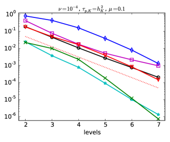
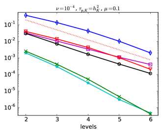
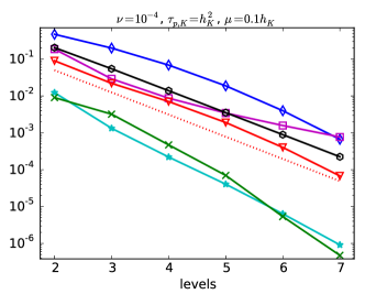
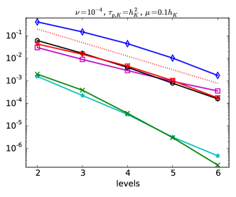
Figure 2: LPS with global grad-div stabilization, $P_{2}/P_{2}$ pair of finite element spaces, Grid 1 (left) and Grid 2 (right), dotted line: slope for second order convergence.

   

   

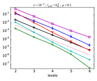
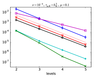
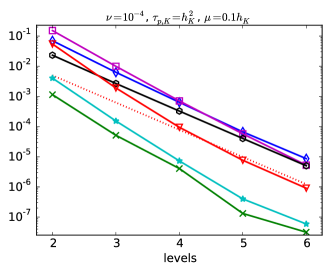
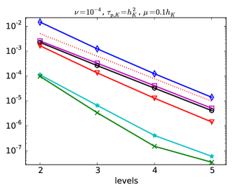
Figure 3: LPS with global grad-div stabilization, $P_{3}/P_{3}$ pair of finite element spaces, Grid 1 (left) and Grid 2 (right), dotted line: slope for third order convergence, same legend as in Figure 2.

Results presented with the $P_{2}/P_{2}$ pair of finite elements are presented in Figure 2 and with the $P_{3}/P_{3}$ pair of spaces in Figure 3. These results agree with the analytical predictions. Concerning the grad-div stabilization parameter there are only minor differences in the results. For the $P_{3}/P_{3}$ pair of spaces, $\mu=0.1h_{K}$ gives a somewhat better approximation of the pressure.

Figure 4 displays a representative result for the dependency of the errors on the viscosity. It can be seen that all errors, in particular the approximation of the error on the left-hand side of (1), are bounded for $\nu\to 0$. This behavior coincides with the analytical prediction.

   

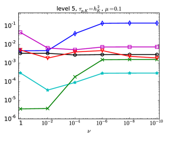
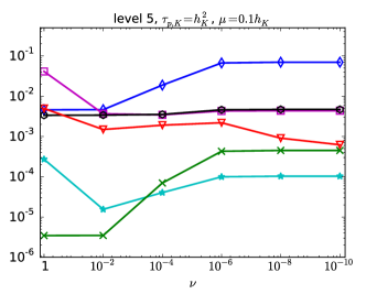
Figure 4: LPS with global grad-div stabilization, $P_{2}/P_{2}$ pair of finite element spaces, Grid 1, behavior of errors with respect to $\nu^{-1}$, same legend as in Figure 2.

7.2 A method with rate of decay $s+1/2$ of the velocity error for $\nu\leq h$

Simulations for the method analyzed in Section 6 were performed on the irregular Grid 2, to prevent any superconvergence effects, for $\nu=10^{-8}$, such that condition (89) is satisfied, and for the final time $T=0.5$. The remaining setup of the simulations was as described in Section 7.1.

The methods incorporating the fluctuations of the velocity gradient were implemented as follows. Generally, the nonlinear problems were solved with a fixed point iteration (Picard iteration). Since the matrix representing the fluctuations of the gradient possesses a wider stencil than all other matrices for the velocity-velocity coupling, we put the term with the fluctuations of the velocity gradient on the right-hand side in the Picard iteration. In order to achieve a satisfying rate of convergence of this iteration, numerical tests showed that the parameters $\{\tau_{\nu,K}\}$ should be rather small. In addition, we could see that increasing these parameters above a certain value leads to a notable increase of the errors. Altogether, for the irregular Grid 2, $\tau_{\nu,K}=0.01h_{K}$ turned out to be an appropriate choice. In view of condition (84), the LPS parameters for the pressure were chosen to be $\tau_{p,K}=10^{-4}h_{K}$.

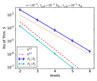
Figure 5: A method with rate of decay $s+1/2$ of the velocity error for $\nu\leq h$, computational results on Grid 2.

An error bound for the considered method was derived in Theorem 5. In the numerical simulations, the terms with the fluctuations on the left-hand side of (5) were approximated by

$$\Delta t\sum_{j=1}^{n}\|\sigma_{h}^{*}(\nabla(I_{h}p^{j}-p_{h}^{j}))\|_{\tau_{p}}^{2},\quad\Delta t\sum_{j=1}^{n}\|\sigma_{h}^{*}(\nabla(I_{h}\boldsymbol{u}^{j}-\boldsymbol{u}_{h}^{j}))\|_{\tau_{\nu}}^{2},$$

where $I_{h}$ is the Lagrangian interpolant. With the interpolants of the solution, these terms can be simply computed by matrix-vector operations with the matrix of the fluctuations.

Computational results are presented in Figure 5. One can observe the proposed rates of decay of the velocity error. Having a detailed look on the individual contributions of the error, we could see that the $L^{2}$ error and the fluctuations of the velocity gradient were dominant.