Unbiased approximations of products of expectations

Abstract

We consider the problem of approximating the product of $n$ expectations with respect to a common probability distribution $\mu$. Such products routinely arise in statistics as values of the likelihood in latent variable models. Motivated by pseudo-marginal Markov chain Monte Carlo schemes, we focus on unbiased estimators of such products. The standard approach is to sample $N$ particles from $\mu$ and assign each particle to one of the expectations. This is wasteful and typically requires the number of particles to grow quadratically with the number of expectations. We propose an alternative estimator that approximates each expectation using most of the particles while preserving unbiasedness. We carefully study its properties, showing that in latent variable contexts the proposed estimator needs only $\mathcal{O}(n)$ particles to match the performance of the standard approach with $\mathcal{O}(n^{2})$ particles. We demonstrate the procedure on two latent variable examples from approximate Bayesian computation and single-cell gene expression analysis, observing computational gains of the order of the number of expectations, i.e. data points, $n$.

Keywords: Latent variable models, Markov chain Monte Carlo, pseudo-marginal, approximate Bayesian computation

1 Introduction

Let $X$ be a random variable with probability measure, or distribution, $\mu$ on a measurable space $(E,\mathcal{E})$, and $L^{1}(\mu)$ the class of integrable, real-valued functions, i.e. $L^{1}(\mu)=\{f:\int_{E}\left|f(x)\right|\mu({\rm d}x)<\infty\}$. For a sequence of non-negative “potential” functions $G_{1},\ldots G_{n}\in L^{1}(\mu)$, we consider approximations of products of $n$ expectations

$$\gamma:=\prod_{p=1}^{n}\mathbb{E}\left[G_{p}(X)\right]=\prod_{p=1}^{n}\mu(G_{p}),$$ (1)

where we denote $\mu(f):=\int_{E}f(x)\mu({\rm d}x)$ for $f\in L^{1}(\mu)$. These arise, e.g., as values of the likelihood function in latent variable models. We concentrate on unbiased approximations of $\gamma$; these can be used, e.g., within pseudo-marginal Markov chain methods for approximating posterior expectations (Beaumont, 2003; Andrieu & Roberts, 2009). To motivate this general problem, and because our main result in the sequel relates to latent variable models, we provide the following generic example of such a model.

Example 1.

Let $g$ be a Markov transition density and $Y_{1},\ldots,Y_{n}$ be i.i.d. $\mathsf{Y}$-valued random variables distributed according to the probability density function $\nu$ where

$$\nu(y):=\mathbb{E}\left[g(X,y)\right]=\int_{E}g(x,y)\mu({\rm d}x),\qquad y\in\mathsf{Y}.$$

That is, the $Y_{p}$ are independent and distributed according to $g(X_{p},\cdot)$ where $X_{p}\sim\mu$. For observations $y_{1},\ldots,y_{n}$, respectively, of $Y_{1},\ldots,Y_{n}$, we can write

$$\prod_{p=1}^{n}\nu(y_{p})=\prod_{p=1}^{n}\mathbb{E}\left[g(X,y_{p})\right]=\prod_{p=1}^{n}\mathbb{E}\left[G_{p}(X)\right]=\gamma,$$

where the potential functions are defined via $G_{p}(x):=g(x,y_{p})$, for $p\in\{1,\ldots,n\}$.

Remark 1.

To see that $\gamma$ can be viewed as a value of the likelihood function, let $\theta\in\Theta$ be a statistical parameter and $\{(\mu_{\theta},g_{\theta}):\theta\in\Theta\}$ parameterized families of distributions and Markov transition densities. The likelihood function $L$ is then $L(\theta):=\prod_{p=1}^{n}\nu_{\theta}(y_{p})$ where

$$\nu_{\theta}(y):=\mathbb{E}\left[g_{\theta}(X,y)\right]=\int_{E}g_{\theta}(x,y)\mu_{\theta}({\rm d}x),\qquad y\in\mathsf{Y},$$

and clearly $L(\theta)$ is of the form (1) for any $\theta\in\Theta$.

The focus of this paper is approximations of $\gamma$ using $N$ independent and $\mu$-distributed random variables $\zeta:=(\zeta_{1},\ldots,\zeta_{N})$, which we will refer to throughout as particles. A straightforward approach to constructing an unbiased approximation of $\gamma$ is to approximate each expectation $\mathbb{E}\left[G_{p}(X)\right]=\mu(G_{p})$ independently using $M$ particles, where $N=Mn$. To be precise, we define

$$\gamma_{{\rm simple}}^{N}:=\prod_{p=1}^{n}\frac{1}{M}\sum_{i=1}^{M}G_{p}(\zeta_{(p-1)M+i}).$$ (2)

We will often refer to the second moment condition

$$\max_{p\in\{1,\ldots,n\}}\mu(G_{p}^{2})<\infty,$$ (3)

and in order to simplify the presentation we define the normalized sequence of potential functions $\bar{G}_{1},\ldots,\bar{G}_{n}$ via $\bar{G}_{p}:=G_{p}/\mu(G_{p})$. The following lack-of-bias, consistency, second moment and variance properties are easily established. We denote convergence in probability by $\overset{P}{\rightarrow}$.

Proposition 1.

We have $\mathbb{E}\left[\gamma_{{\rm simple}}^{N}\right]=\gamma$, $\gamma_{{\rm simple}}^{N}\overset{P}{\rightarrow}\gamma$ as $N\rightarrow\infty$ and

$$\mathbb{E}\left[\left(\gamma_{{\rm simple}}^{N}/\gamma\right)^{2}\right]=\prod_{p=1}^{n}\left\{1+\left[\mu(\bar{G}_{p}^{2})-1\right]/M\right\},$$ (4)

so ${\rm var}(\gamma_{{\rm simple}}^{N})$ is finite and converges to $0$ as $M\rightarrow\infty$ if and only if (3) holds.

The approximation $\gamma_{{\rm simple}}^{N}$ is straightforward to compute and analyze since it is a product of averages of independent random variables. However, each particle is only used to approximate one of the expectations in the product, and in situations where these particles are expensive to obtain this may be wasteful. An alternative approach is to use

$$\gamma_{{\rm biased}}^{N}:=\prod_{p=1}^{n}\frac{1}{N}\sum_{i=1}^{N}G_{p}(\zeta_{i}),$$ (5)

which is consistent and not wasteful, but also not unbiased in general.

Proposition 2.

We have $\gamma_{{\rm biased}}^{N}\overset{P}{\rightarrow}\gamma$ as $N\rightarrow\infty$ but $\mathbb{E}\left[\gamma_{{\rm biased}}^{N}\right]\neq\gamma$ in general.

We propose in the sequel an approximation $\gamma_{{\rm recycle}}^{N}$ that is unbiased like $\gamma_{{\rm simple}}^{N}$ but which is closer to $\gamma_{{\rm biased}}^{N}$ in that it uses most of the particles to approximate each expectation in the product while remaining computationally tractable. The approximation $\gamma_{{\rm recycle}}^{N}$ can be viewed as an unbiased approximation of $\gamma_{{\rm perm}}^{N}$, the rescaled permanent of a particular rectangular matrix of random variables, which is never worse in terms of variance than $\gamma_{{\rm simple}}^{N}$ but is very computationally costly to compute in general. The approximation $\gamma_{{\rm recycle}}^{N}$ is an extension of the importance sampling approximation of the permanent of a square matrix proposed by Kuznetsov (1996) to the case of rectangular matrices. While it is possible for $\gamma_{{\rm recycle}}^{N}$ to have a higher variance than $\gamma_{{\rm simple}}^{N}$, we show that in many statistical scenarios it requires far fewer particles to obtain a given variance, e.g. in the latent variable setting described above. In particular, under weak assumptions, one needs to take $N=\mathcal{O}(n)$ to control the relative variance of $\gamma_{{\rm recycle}}^{N}$ but one requires $N=\mathcal{O}(n^{2})$ to control the relative variance of $\gamma_{{\rm simple}}^{N}$.

The paper is structured as follows. In Section 2 we draw the connection with matrix permanents, define the proposed estimator $\gamma_{{\rm recycle}}^{N}$, and analyze basic properties such as unbiasedness and consistency. In Section 3 we compare the behavior of $\gamma_{{\rm simple}}^{N}$ and $\gamma_{{\rm recycle}}^{N}$ as $n$ increases under various assumptions on the potential functions, while in Section 4 we consider latent variable models. Finally, Section 5 provides simulation studies showing the effect of using $\gamma_{{\rm recycle}}^{N}$ rather than $\gamma_{{\rm simple}}^{N}$ in pseudo-marginal Markov chain Monte Carlo methods for estimating the parameters of a g-and-k model, commonly used as a test application for approximate Bayesian computation methodology, and of a Poisson-Beta model for single-cell gene expression. In both cases we observe computational speedups of the order of the number of data points $n$. Section 6 provides a discussion and potential future works. All proofs are housed in the appendix or the supplementary materials.

2 The associated permanent and its approximation

For integers $i\leq j$ we denote $\left\llbracket i,j\right\rrbracket=\{i,\ldots,j\}$. We adopt the convention that $\prod_{j\in\emptyset}G_{j}=1$, and will occasionally use the notation $x_{p:q}=(x_{p},\ldots,x_{q})$ for $p,q\in\mathbb{N}$ with $p\leq q$. An alternative approximation of $\gamma$ on the basis of the particles $\zeta=(\zeta_{1},\ldots,\zeta_{N})$ is obtained by first rewriting $\gamma$ in (1) as, with $X_{1},\ldots,X_{p}$ independent $\mu$-distributed random variables,

$$\gamma=\prod_{p=1}^{n}\mathbb{E}\left[G_{p}(X)\right]=\mathbb{E}\left[\prod_{p=1}^{n}G_{p}(X_{p})\right].$$

Indeed, $\gamma_{{\rm biased}}^{N}$ is a V-statistic of order $n$ for $\gamma$, and the corresponding U-statistic for $\gamma$ is

$$\gamma_{{\rm perm}}^{N}:=\sum_{k\in P(N,n)}\left|P(N,n)\right|^{-1}\prod_{p=1}^{n}G_{p}(\zeta_{k_{p}}),$$ (6)

where $P(N,n)=\{k\in\left\llbracket 1,N\right\rrbracket^{n}:k_{i}=k_{j}\iff i=j\}$ is the set of $n$-permutations of $N$, whose cardinality is $\left|P(N,n)\right|=N!/(N-n)!$. We observe that $\gamma_{{\rm perm}}^{N}$ is exactly $\left|P(N,n)\right|^{-1}$ times the permanent of the rectangular matrix $A$ (see, e.g., Ryser, 1963, p. 25) with entries $A_{ij}=G_{i}(\zeta_{j})$ since then

$${\rm perm}(A)=\sum_{k\in P(N,n)}\prod_{p=1}^{n}A_{p,k_{p}}=\sum_{k\in P(N,n)}\prod_{p=1}^{n}G_{p}(\zeta_{k_{p}}).$$

The approximation $\gamma_{{\rm perm}}^{N}$ is unbiased and consistent since it is a U-statistic and moreover it is less variable than $\gamma_{{\rm simple}}^{N}$ in terms of the convex order (see, e.g., Shaked & Shanthikumar, 2007, Section 3.A), defined by $X\preceq_{{\rm cx}}Y$ if $\mathbb{E}\left[\phi(X)\right]\leq\mathbb{E}\left[\phi(Y)\right]$ for all convex functions $\phi:\mathbb{R}\rightarrow\mathbb{R}$ such that the expectations are well-defined. Since $x\mapsto x$ and $x\mapsto-x$ are convex functions, convex-ordered random variables necessarily have the same expectation, and since $x\mapsto x^{2}$ is convex, $X\preceq_{{\rm cx}}Y$ implies ${\rm var}(X)\leq{\rm var}(Y)$. Convex-ordered families of random variables also allow one to order the asymptotic variances of associated pseudo-marginal Markov chains (Andrieu & Vihola, 2016, Theorem 10). In order to express the second moments of $\gamma_{{\rm perm}}^{N}/\gamma$ and $\gamma_{{\rm recycle}}^{N}/\gamma$, we define the function $\psi_{N}:\left\llbracket 1,N\right\rrbracket^{n}\rightarrow\mathbb{R}_{+}$ by

$$\psi_{N}(r):=\left\{\prod_{p=1}^{n}\mu(\bar{G}_{p}\prod_{j:r_{j}=p}\bar{G}_{j})\right\}\left\{\prod_{i=n+1}^{N}\mu(\prod_{j:r_{j}=i}\bar{G}_{j})\right\},\qquad r\in\left\llbracket 1,N\right\rrbracket^{n},$$ (7)

where $fg$ denotes pointwise product so that $\mu(fg)=\int f(x)g(x)\mu({\rm d}x)$. We now state basic properties of $\gamma_{{\rm perm}}^{N}$, which can be compared with Proposition 1.

Theorem 1.

The following hold:

1. $\mathbb{E}[\gamma_{{\rm perm}}^{N}]=\gamma$ and $\gamma_{{\rm perm}}^{N}\preceq_{{\rm cx}}\gamma_{{\rm simple}}^{N}$.

2. $\gamma_{{\rm perm}}^{N}\overset{P}{\rightarrow}\gamma$ as $N\rightarrow\infty$.

3. The second moment of $\gamma_{{\rm perm}}^{N}/\gamma$ is, with $K\sim{\rm Uniform}(P(N,n))$,

   $$\mathbb{E}[(\gamma_{{\rm perm}}^{N}/\gamma)^{2}]=\mathbb{E}[\prod_{p=1}^{n}\bar{G}_{p}(\zeta_{p})\bar{G}_{p}(\zeta_{K_{p}})]=\mathbb{E}\left[\psi_{N}(K)\right]=\mathbb{E}[\prod_{p=1}^{n}\mu\big{(}\bar{G}_{p}\prod_{j:K_{j}=p}\bar{G}_{j}\big{)}].$$

4. ${\rm var}(\gamma_{{\rm perm}}^{N})$ is finite and ${\rm var}(\gamma_{{\rm perm}}^{N})\rightarrow 0$ as $N\rightarrow\infty$ if and only if (3) holds.

This suggests that $\gamma_{{\rm perm}}^{N}$ is a superior approximation of $\gamma$ in comparison to $\gamma_{{\rm simple}}^{N}$. However, computing $\gamma_{{\rm perm}}^{N}$ is equivalent to computing the permanent of a rectangular matrix, which has no known polynomial-time algorithm. In fact, computing the permanent of a square matrix is #P-hard (Valiant, 1979). Using an extension of the importance sampling estimator of the permanent of a square matrix due to Kuznetsov (1996), we define the following unbiased approximation of $\gamma_{{\rm perm}}^{N}$ and hence $\gamma$,

$$\gamma_{{\rm recycle}}^{N}:=\prod_{p=1}^{n}\frac{1}{N-p+1}\sum_{j=1}^{N}G_{p}(\zeta_{j})\mathbb{I}\left(j\notin\{K_{1},\ldots,K_{p-1}\}\right),$$ (8)

where $K:=(K_{1},\ldots,K_{n})$ is a $\left\llbracket 1,N\right\rrbracket^{n}$-valued random variable whose distribution given $\zeta$ is defined by the sequence of conditional probabilities

$$\mathbb{P}\left[K_{p}=i\mid\zeta,K_{1},\ldots,K_{p-1}\right]\propto G_{p}(\zeta_{i})\mathbb{I}\left(i\notin\{K_{1},\ldots,K_{p-1}\}\right).$$ (9)

In (9) we take $G_{p}(\zeta_{i})/\sum_{j=1}^{N}G_{p}(\zeta_{j})\mathbb{I}\left(j\notin\{K_{1},\ldots,K_{p-1}\}\right)$ to be $1$ when the denominator is equal to $0$. That is, when the denominator is $0$, then $K_{p}\mid(\zeta,K_{1},\ldots,K_{p-1})\sim{\rm Uniform}(\left\llbracket 1,N\right\rrbracket\setminus\{K_{1},\ldots,K_{p-1}\})$. The choice of the conditional distribution of $K_{p}$ when $\sum_{j=1}^{N}G_{p}(\zeta_{j})\mathbb{I}\left(j\notin\{K_{1},\ldots,K_{p-1}\}\right)=0$ is in some sense arbitrary, as in any case $\gamma_{{\rm recycle}}^{N}=0$ whenever this happens. We now state basic properties of $\gamma_{{\rm recycle}}^{N}$, which can be compared with Theorem 1.

Algorithm 1 Computing $\gamma_{{\rm recycle}}^{N}$

1. Sample $\zeta_{1},\ldots,\zeta_{N}\sim\mu$ independently, and set $Z_{0}\leftarrow 1$.

2. For $p=1,\ldots,n$:

   1. Set $Z_{p}\leftarrow Z_{p-1}\sum_{j=1}^{N}G_{p}(\zeta_{j})\mathbb{I}\left(j\notin\{K_{1},\ldots,K_{p-1}\}\right)/(N-p+1)$.

   2. Sample $K_{p}\mid(K_{1},\ldots,K_{p-1})$ according to (9).

3. Set $\gamma_{{\rm recycle}}^{N}\leftarrow Z_{n}$.

Theorem 2.

The following hold:

1. $\mathbb{E}\left[\gamma_{{\rm recycle}}^{N}\mid\zeta\right]=\gamma_{{\rm perm}}^{N}$, $\mathbb{E}\left[\gamma_{{\rm recycle}}^{N}\right]=\gamma$ and $\gamma_{{\rm perm}}^{N}\preceq_{{\rm cx}}\gamma_{{\rm recycle}}^{N}$.

2. $\gamma_{{\rm recycle}}^{N}\overset{P}{\rightarrow}\gamma$ as $N\rightarrow\infty$.

3. Let $S=(S_{1},\ldots,S_{n})$ be a vector of independent random variables with $S_{p}\sim{\rm Uniform}(\left\llbracket p,N\right\rrbracket)$ for $p\in\left\llbracket 1,n\right\rrbracket$. The second moment of $\gamma_{{\rm recycle}}^{N}/\gamma$ is

   $$\mathbb{E}\left[(\gamma_{{\rm recycle}}^{N}/\gamma)^{2}\right]=\mathbb{E}[\prod_{p=1}^{n}\bar{G}_{p}(\zeta_{p})\bar{G}_{p}(\zeta_{S_{p}})]=\mathbb{E}\left[\psi_{N}(S)\right].$$

4. ${\rm var}(\gamma_{{\rm recycle}}^{N})$ is finite and ${\rm var}(\gamma_{{\rm recycle}}^{N})\rightarrow 0$ as $N\rightarrow\infty$ if and only if

   $$\max_{p\in\left\llbracket 1,n\right\rrbracket,\>B\subseteq\left\llbracket 1,p\right\rrbracket}\mu(G_{p}\prod_{j\in B}G_{j})<\infty.$$ (10)

Corollary 1.

If $\max_{p\in\left\llbracket 1,n\right\rrbracket}\mu(G_{p}^{n+1})<\infty$ then ${\rm var}(\gamma_{{\rm recycle}}^{N})\rightarrow 0$ as $N\rightarrow\infty$.

Remark 2.

We observe that $\mathbb{E}[(\gamma_{{\rm perm}}^{N}/\gamma)^{2}]=\mathbb{E}\left[\psi_{N}(K)\right]\leq\mathbb{E}\left[\psi_{N}(S)\right]=\mathbb{E}[(\gamma_{{\rm recycle}}^{N}/\gamma)^{2}]$, where $K$ and $S$ are defined in the statements of Theorems 1 and 2, respectively.

Remark 3.

While (3) is sufficient for $\gamma_{{\rm perm}}^{N}$ and $\gamma_{{\rm simple}}^{N}$ to have finite variance converging to $0$ as $N\rightarrow\infty$, this is not sufficient in general for $\gamma_{{\rm recycle}}^{N}$, which requires (10) instead.

The estimator $\gamma_{{\rm simple}}^{N}$ uses only $N/n$ out of $N$ particles to estimate each expectation in the product; in contrast $\gamma_{{\rm recycle}}^{N}$ uses $N-p$ particles for the $p$th expectation $\mu(G_{p})$. In this sense, the latter recycles most of the particles for each term, and we therefore refer to $\gamma_{{\rm recycle}}^{N}$ as the recycled estimator in the sequel. While Remark 3 implies that it is not possible for ${\rm var}(\gamma_{{\rm recycle}}^{N})\leq{\rm var}(\gamma_{{\rm simple}}^{N})$ in general, we show in the coming section that ${\rm var}(\gamma_{{\rm recycle}}^{N})$ can be orders of magnitude smaller than ${\rm var}(\gamma_{{\rm simple}}^{N})$ in many statistical settings.

3 Scaling of the number of particles with $n$

We investigate the variance of $\gamma_{{\rm recycle}}^{N}$ in comparison to $\gamma_{{\rm simple}}^{N}$ in the large $n$ regime. In particular, we show that only $N=\mathcal{O}(n)$ particles are required to control the relative variance of $\gamma_{{\rm recycle}}^{N}$ in some scenarios in which $N=\mathcal{O}(n^{2})$ particles are required to control the relative variance of $\gamma_{{\rm simple}}^{N}$. We also show that this cannot always be true, in some situations $N=\mathcal{O}(n^{2})$ is a lower bound on the number of particles required to control the relative variance of $\gamma_{{\rm perm}}^{N}$, and therefore $\gamma_{{\rm recycle}}^{N}$. To simplify the presentation, we define $c_{p}:=\mu(\bar{G}_{p}^{2})-1$, for $p\in\left\llbracket 1,n\right\rrbracket$. We will occasionally make reference to the following assumption when considering the large $n$ regime

$$1<\inf_{p\geq 1}c_{p}\leq\sup_{p\geq 1}c_{p}<\infty.$$ (11)

We begin by observing that from Proposition 1, if (11) holds and $M=\left\lceil\alpha n^{\beta}\right\rceil$ then the second moment of $\gamma_{{\rm simple}}^{N}/\gamma$ is bounded above as $n\rightarrow\infty$ if and only if $\alpha>0$ and $\beta\geq 1$. Since $N=Mn$, this implies that to stabilize the relative variance of $\gamma_{{\rm simple}}^{N}$ in the large $n$ regime one must take $N=\mathcal{O}(n^{2})$.

The second moment of $\gamma_{{\rm recycle}}^{N}/\gamma$ is more complex to analyze because it involves interactions between different potential functions. The following results consider three particular situations. The first is a favorable scenario, in which it follows that if $N=\alpha n$ for $\alpha>1$ and (11) holds with $c=\sup_{p\geq 1}c_{p}$, then $\mathbb{E}[(\gamma_{{\rm recycle}}^{N}/\gamma)^{2}]\leq\exp\left(c/\left[\alpha-1\right]\right)$.

Proposition 3.

Assume $G_{1}(X),\ldots,G_{n}(X)$ are mutually independent when $X\sim\mu$. Then

$$\mathbb{E}\left[\left(\gamma_{{\rm recycle}}^{N}/\gamma\right)^{2}\right]=\prod_{p=1}^{n}\left[1+c_{p}/(N-p+1)\right].$$ (12)

The second scenario is also favorable: if the potential functions are negatively correlated in a specific sense, $\gamma_{{\rm recycle}}^{N}=\gamma_{{\rm perm}}^{N}$ and again it is sufficient to take $N=\mathcal{O}(n)$ to control the second moment of $\gamma_{{\rm recycle}}^{N}/\gamma$.

Proposition 4.

Assume that for any distinct $p,q\in\left\llbracket 1,n\right\rrbracket$, $G_{p}(X)G_{q}(X)=0$ almost surely. Then $\gamma_{{\rm recycle}}^{N}=\gamma_{{\rm perm}}^{N}$ almost surely, and $\mathbb{E}\left[(\gamma_{{\rm recycle}}^{N}/\gamma)^{2}\right]\leq\prod_{p=1}^{n}\left[1+c_{p}/(N-p+1)\right]$.

The third scenario is not favorable, corresponding to the case where the potential functions are identical. At least a quadratic in $n$ number of particles is required to control $\mathbb{E}[(\gamma_{{\rm recycle}}^{N}/\gamma)^{2}]$ in this setting. Loosely speaking, positive correlations between $G_{p}(X)$ and $G_{q}(X)$ tend to increase the second moment of $\gamma_{{\rm recycle}}^{N}/\gamma$, while correlations have no effect on the second moment of $\gamma_{{\rm simple}}^{N}/\gamma$. Nevertheless, we show in Proposition 6 that when the moments of $\bar{G}_{1}(X)$ increase no more quickly than those associated to rescaled Bernoulli random variables, $\gamma_{{\rm recycle}}^{N}$ has a smaller variance than $\gamma_{{\rm simple}}^{N}$. Hence the recycled estimator may be useful, even if not orders of magnitude better, in some applications involving the same potential functions, e.g. the Poisson estimator of Beskos et al. (2006), based on general methods by Bhanot & Kennedy (1985) and Wagner (1988).

Proposition 5.

Assume $G_{1}=\cdots=G_{n}$. Then $\mathbb{E}\left[(\gamma_{{\rm recycle}}^{N}/\gamma)^{2}\right]\geq\mathbb{E}\left[(\gamma_{{\rm perm}}^{N}/\gamma)^{2}\right]\geq(1+c_{1})^{n^{2}/N}$.

Proposition 6.

Let $G_{1}=\cdots=G_{n}$ and assume that $\mu(\bar{G}_{1}^{\ell})\leq\mu(\bar{G_{1}}^{2})^{\ell-1}$ for $\ell\in\left\llbracket 3,n\right\rrbracket$. Then $\mathbb{E}\left[(\gamma_{{\rm recycle}}^{N}/\gamma)^{2}\right]\leq\mathbb{E}\left[(\gamma_{{\rm simple}}^{N}/\gamma)^{2}\right]$.

Our final general result is motivated by approximate Bayesian computation applications, in which it is often the case that the potential functions are indicator functions. In this case, it is also true that $\gamma_{{\rm recycle}}^{N}$ has a smaller variance than $\gamma_{{\rm simple}}^{N}$.

Proposition 7.

Let $A_{1},\ldots,A_{n}\in\mathcal{E}$ satisfy $\mu(A_{p})>0$ for $p\in\left\llbracket 1,n\right\rrbracket$. Let $G_{p}:=\mathbb{I}{}_{A_{p}}$ for $p\in\left\llbracket 1,n\right\rrbracket$. Then $\mathbb{E}\left[(\gamma_{{\rm recycle}}^{N}/\gamma)^{2}\right]\leq\mathbb{E}\left[(\gamma_{{\rm simple}}^{N}/\gamma)^{2}\right]$.

Remark 4.

An alternative approximation of $\gamma$ can be obtained by sampling a number of permutations $\sigma_{1},\ldots,\sigma_{q}$ of $\left\llbracket 1,n\right\rrbracket$ and calculating $\gamma_{{\rm simple}}^{N}$ using each permutation. That is, if we define

$$\gamma_{{\rm simple}}^{N}(\sigma)=\prod_{p=1}^{n}\frac{1}{M}\sum_{i=1}^{M}G_{p}(\zeta_{\sigma((p-1)M+i)}),$$

then $q^{-1}\sum_{i=1}^{q}\gamma_{{\rm simple}}^{N}(\sigma_{i})$ is also an approximation of $\gamma_{{\rm perm}}^{N}$ and hence $\gamma$. This strategy does not scale well with $n$, however. For example, if (11) holds and $M=\left\lceil\alpha n^{\beta}\right\rceil$ with $\alpha>0$ and $\beta\in(0,1)$ we require $q$ to grow exponentially with $n$ to stabilize the relative variance of $q^{-1}\sum_{i=1}^{q}\gamma_{{\rm simple}}^{N}(\sigma_{i})$. The crucial observation to establish this is that for non-negative random variables $W_{1},\ldots,W_{q}$ with identical means and variances, we have $\mathbb{E}\left[(q^{-1}\sum_{i=1}^{q}W_{i})^{2}\right]\geq q^{-1}\mathbb{E}\left[W_{1}^{2}\right]$, and the argument follows from Proposition 1.

4 Latent variable models

The assumption of mutual independence in Proposition 3 is very strong in statistical settings. However, we show now that in latent variable models the expected second moment of $\gamma_{{\rm recycle}}^{N}/\gamma$ is very similar to (12), where the expectation $\mathsf{E}$ is w.r.t. the law of the observations $Y_{1},\ldots,Y_{n}\overset{i.i.d.}{\sim}\nu$. For the remainder of this section, we denote by $\bar{G}_{1}$ the random function $x\mapsto g(x,Y_{1})/\nu(Y_{1})$ for $Y_{1}\sim\nu$. We begin by verifying (10) for latent variable models under a finite expected second moment condition for $\bar{G}_{1}(X)$ when $X\sim\mu$. This condition has appeared in the literature in a variety of places, see e.g. Breiman & Friedman (1985), Buja (1990), Schervish & Carlin (1992), Liu et al. (1995) and Khare & Hobert (2011).

Proposition 8.

In the setting of Example 1, assume that $\mathsf{E}\left[\mu(\bar{G}_{1}^{2})\right]<\infty$. If $Y_{1},\ldots,Y_{n}\overset{i.i.d.}{\sim}\nu_{0}$ where $\nu_{0}$ is absolutely continuous with respect to $\nu$, then (10) holds almost surely.

The following Theorem is our main result in terms of applicability to statistical scenarios. It suggests that when considering the expected second moment of $\gamma_{{\rm recycle}}^{N}/\gamma$, it is as if the random variables $G_{1}(X),\ldots,G_{n}(X)$ are “mutually independent on average”, and allows easy comparison with the corresponding expected second moment of $\gamma_{{\rm simple}}^{N}/\gamma$.

Theorem 3.

In the setting of Example 1, and letting $\mathsf{E}$ denoting expectation w.r.t. $Y_{1},\ldots,Y_{n}$,

$$\mathsf{E}\left[\mathbb{E}\left[\left(\gamma_{{\rm recycle}}^{N}/\gamma\right)^{2}\right]\right]=\prod_{p=1}^{n}\left[1+C/(N-p+1)\right],\qquad C=\mathsf{E}\left[\mu(\bar{G}_{1}^{2})\right]-1.$$

Remark 5.

In the setting of Example 1, it is straightforward to obtain from Proposition 1 that $\mathsf{E}[\mathbb{E}[(\gamma_{{\rm simple}}^{N}/\gamma)^{2}]]=\left(1+C/M\right)^{n}$, where $C$ is as in Theorem 3. Hence, one requires $N=\left\lceil\alpha n\right\rceil$ for $\alpha>1$ to control the expected relative variance of $\gamma_{{\rm recycle}}^{N}$ but one requires $M=\mathcal{O}(n)$ and hence $N=\mathcal{O}(n^{2})$ to control the expected relative variance of $\gamma_{{\rm simple}}^{N}$ when $1<C<\infty$. In addition, it is clear that $\mathsf{E}[\mathbb{E}[(\gamma_{{\rm recycle}}^{N}/\gamma)^{2}]]<\mathsf{E}[\mathbb{E}[(\gamma_{{\rm simple}}^{N}/\gamma)^{2}]]$ for any $N$ that is an integer multiple of $n>1$.

Remark 6.

The condition $\mathsf{E}\left[\mu(\bar{G}_{1}^{2})\right]<\infty$ is not very strong, but is not always satisfied. For example, if $\mu$ is ${\rm Uniform}(0,1)$ and $g(x,\cdot)$ is ${\rm Uniform}(0,x)$ for each $x\in(0,1)$ then simple calculations show that $\mathsf{E}\left[\mu(\bar{G}_{1}^{2})\right]=\infty$.

5 Applications

We consider Bayesian inference in two latent variable model applications, employing $\gamma_{{\rm recycle}}^{N}$ or $\gamma_{{\rm simple}}^{N}$ to approximate $L(\theta)$ in a pseudo-marginal version of a random-walk Metropolis Markov chain. General guidelines for tuning the value of $N$ in such chains have been proposed by Doucet et al. (2015) and Sherlock et al. (2015), who suggest that one should choose $N$ such that the relative variance of the estimator is roughly $2$. While the relative variance typically varies with $\theta$, if the posterior distribution for $\theta$ is reasonably concentrated near the true parameter $\theta_{0}$, in practice one can often choose $N$ so that the estimator has a relative variance of $2$ at some point close to $\theta_{0}$. In both applications below, following Roberts & Rosenthal (2001), we tune the proposal for the random-walk Metropolis algorithm using a shorter run of the Markov chain. Specifically, we choose the proposal density

$$q(\theta,\theta^{\prime})=\mathcal{N}(\theta^{\prime};\theta,d^{-1/2}2.38\hat{\Sigma}),$$

where $\hat{\Sigma}$ is the estimated covariance matrix of the posterior distribution and $\theta\in\mathbb{R}^{d}$. All computations were performed in the R programming language with C++ code accessed via the ‘Rcpp’ package (Eddelbuettel & François, 2011). Effective sample sizes were computed using the ‘mcmcse’ package (Flegal et al., 2017).

Using $\gamma_{{\rm perm}}^{N}$ instead of $\gamma_{{\rm simple}}^{N}$ to approximate each $L(\theta)$ in a pseudo-marginal Markov chain can only decrease the asymptotic variance of ergodic averages of functions $\varphi$ with ${\rm var}_{\pi}(\varphi)<\infty$. This is a consequence of Andrieu & Vihola (2016, Theorem 10) and Theorem 1. Using $\gamma_{{\rm recycle}}^{N}$ does not have the same guarantee in general, but Theorem 3 suggests that if the estimators perform similarly for a set of $\theta$ with large posterior mass, then this should result in greatly improved performance over $\gamma_{{\rm simple}}^{N}$ for large $n$.

5.1 Approximate Bayesian computation: g-and-k model

Approximate Bayesian computation (ABC) is a branch of simulation-based inference used when the likelihood function cannot be evaluated pointwise but one can simulate from the model for any value of the statistical parameter. While there are a number of variants, in general the methodology involves comparing a summary statistic associated with the observed data with summary statistics associated with pseudo-data simulated using different parameter values (see Marin et al., 2012, for a recent review). When the data are modelled as $n$ observations of i.i.d.  random variables with distribution $\mu$, it is commonplace to summarize the data using some fixed-dimensional summary statistic independent of $n$, for computational rather than statistical reasons. This summarization, or dimension reduction, can in principle involve little loss of information about the parameters — in exponential families sufficient statistics of fixed dimension exist and could be computed or approximated — but in practice this is not always easy to achieve. An alternative approach that we adopt here is to eschew dimension reduction altogether and treat the model as a standard latent variable model, essentially using the noisy ABC methodology of Fearnhead & Prangle (2012). This may be viewed as an alternative to the construction of summaries using the Wasserstein distance recently proposed by Bernton et al. (2017). One possible outcome of this is that less data may be required to achieve a given degree of posterior concentration; a theoretical treatment of this is beyond the scope of this paper.

The $g$-and-$k$ distribution has been used as an example application for ABC methods since Allingham et al. (2009). The distribution is parameterized by $\theta=(A,B,g,k)$ and a sample $X$ from this distribution can be expressed as

$$X=A+B\left\{1+c\frac{1-\exp(-gZ)}{1+\exp(-gZ)}\right\}\left\{1+Z^{2}\right\}^{k}Z,$$

where $Z\sim\mathcal{N}(0,1)$ is a standard normal random variable and we fix the value $c=4/5$. We consider here observations $y_{1},\ldots,y_{n}$ of $n$ independent random variables $Y_{i}=X_{i}+\epsilon U_{i}$ where $X_{i}\overset{i.i.d.}{\sim}g\text{-and-}k(\theta_{0})$ and $U_{i}\overset{i.i.d.}{\sim}{\rm Uniform}(-\epsilon,\epsilon)$ with $\theta_{0}=(3,1,2,0.5)$ and $\epsilon=1/5$. The values of $c$ and $\theta_{0}$ follow Allingham et al. (2009). We let $\mu_{\theta}$ denote the distribution of $X\sim g\text{-and-}k(\theta)$, and define $G_{p}=\mathbb{I}_{(y_{p}-\epsilon,y_{p}+\epsilon)}$, so that $\gamma(\theta)=\prod_{p=1}^{n}\mu_{\theta}(G_{p})$ is equivalent to the likelihood $L(\theta)$ associated with $\theta$. We take $n=100$ and, following Allingham et al. (2009), we put independent ${\rm Uniform}(0,10)$ priors on each component of $\theta$. In order to have a relative variance of $\gamma_{{\rm recycle}}^{N}(\theta_{0})$ of roughly $2$, it was sufficient to take $N=100n=10^{4}$ whereas for $\gamma_{{\rm simple}}^{N}(\theta_{0})$ we required $N=100n^{2}=10^{6}$. Using both estimators resulted in very similar Markov chains, but the computational cost of using the simple estimator was over $30$ times greater; it took $25.6$ hours to simulate a simple chain of length $10^{6}$ and $8.4$ hours to simulate a recycled chain of length $10^{7}$. It would have taken over $10$ days to simulate a simple chain of length $10^{7}$. Figure 1 shows posterior density estimates associated with the recycled chain; effective sample sizes for each component were above $80,000$. In this example, simulating from $\mu$ is approximately $1200$ times more expensive than evaluating a potential function. Finally, we observe that the posterior distribution for $\theta$ places most of its mass near $\theta_{0}$ despite using $n=100$; in contrast Allingham et al. (2009) used $n=10^{5}$ and Figure 1 shows more concentration overall and better identification of the $g$ parameter than their Figure 3. This suggests that this type of latent variable approach may be preferable to dimension-reducing summaries in some i.i.d. ABC models.

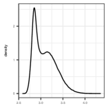
(a) $A$

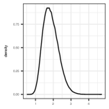
(b) $B$

(c) $g$

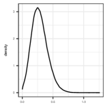
(d) $k$

Figure 1: Posterior density estimates for $\theta$ for the g-and-k model.

5.2 Poisson-Beta model for gene expression

Peccoud & Ycart (1995) proposed a continuous-time birth-and-death process in a random environment to model single-cell gene expression levels; this model enjoys strong experimental support (Delmans & Hemberg, 2016). Letting $V=(V_{t})_{t\geq 0}$ denote the $\mathbb{Z}_{+}$-valued process counting the amount of transcribed mRNA and $W=(W_{t})_{t\geq 0}$ denote the $\{0,1\}$-valued process indicating whether the gene is inactive or active, the Markov process $X=(X_{t})_{t\geq 0}=(V,W)$ is described by, with $X_{t}=(v,w)$,

$$\mathbb{P}\left[X_{t+dt}=(v^{\prime},w^{\prime})\right]=\begin{cases}v\,dt+o(dt)&(v^{\prime},w^{\prime})=(v-1,w),\\ {}[k_{{\rm on}}(1-w)+k_{{\rm off}}w]\,dt+o(dt)&(v^{\prime},w^{\prime})=(v,1-w),\\ \lambda\,dt+o(dt)&(v^{\prime},w^{\prime},w)=(v+1,1,1),\\ 0&\text{otherwise}.\end{cases}$$

The statistical parameters $k_{{\rm on}}$, $k_{{\rm off}}$ and $\lambda$ are respectively the rates at which: the gene switches from inactive to active, the gene switches from active to inactive, and, mRNA is transcribed when the gene is active. The rate of mRNA degradation is assumed here to be $1$. Peccoud & Ycart (1995) derive the probability generating function of the stationary distribution of this process, from which one obtains the probability mass function of the stationary marginal distribution of $V$

$$\mu(v)=\frac{\lambda^{v}\int_{0}^{1}t^{k_{{\rm on}}+v-1}(1-t)^{k_{{\rm off}}-1}e^{-\lambda t}\,dt}{v!\>{\rm Beta}(k_{{\rm on}},k_{{\rm off}})},\qquad v\in\mathbb{Z}_{+}.$$

As observed by, e.g., Kim & Marioni (2013), straightforward calculations provide that this is equivalent to the probability mass function of $X\sim\text{Poisson-Beta}(\lambda,k_{{\rm on}},k_{{\rm off}})$, defined hierarchically by $X\mid S\sim{\rm Poisson}(\lambda S)$ where $S\sim{\rm Beta}(k_{{\rm on}},k_{{\rm off}})$. This model was also mentioned in Wills et al. (2013), who described the Poisson-Beta model directly.

In an experiment, one might observe in the stationary regime mRNA counts with noise for $n$ independent cells, which can therefore be modelled as $n$ independent random variables $Y_{1},\ldots,Y_{n}$ with distribution $Y_{i}=X_{i}+\sigma Z_{i}$ where $X_{i}\overset{{\rm ind}}{\sim}\text{Poisson-Beta}(\lambda,k_{{\rm on}},k_{{\rm off}})$ and $Z_{1},\ldots,Z_{n}$ are independent standard normal random variables. Hence, this can be viewed as a latent variable model with $\theta=(\lambda,k_{{\rm on}},k_{{\rm off}})$, $\mu_{\theta}=\text{Poisson-Beta}(\theta)$ and $G_{p}(x)=\mathcal{N}(y_{p};x,\sigma^{2})$, and likelihood function values $L(\theta)$ are exactly of the form described in Remark 1. We simulated data $y_{1},\ldots,y_{n}$ with $n=1000$, $\theta_{0}=(500,2,8)$ and $\sigma=5$, and proceeded to conduct Bayesian inference via pseudo-marginal MCMC with independent exponential priors on $\lambda$, $k_{{\rm on}}$ and $k_{{\rm off}}$ with means of $1000$, $10$ and $10$, respectively. In order to have a relative variance of $\gamma_{{\rm recycle}}^{N}(\theta_{0})$ of roughly $2$, it was sufficient to take $N=20n=2\times 10^{4}$ whereas for $\gamma_{{\rm simple}}^{N}(\theta_{0})$ we required $N=20n^{2}=2\times 10^{7}$. Using both estimators resulted in very similar Markov chains, but the computational cost of using the simple estimator was approximately $600$ times greater; it took $12.25$ hours to simulate a simple chain of length $10^{4}$ and $6.15$ hours to simulate a recycled chain of length $3\times 10^{6}$. It would have taken over $153$ days to simulate a simple chain of length $3\times 10^{6}$. Figure 2 shows posterior density estimates associated with the recycled chain; effective sample sizes for each component were above $23,000$. In this example, simulating from $\mu$ is approximately $2700$ times more expensive than evaluating a potential function.

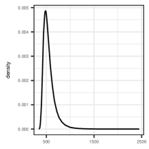
(a) $\lambda$

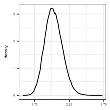
(b) $k_{{\rm on}}$

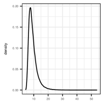
(c) $k_{{\rm off}}$

Figure 2: Posterior density estimates for $\theta$ for the Poisson-Beta model.

6 Discussion

We have proposed an unbiased estimator of a product of expectations that involves using, or recycling, most of the random variables simulated. This results in considerable decreases in the computational time required to approximate such a product accurately when the number of terms in the product, $n$, is large and the computational cost of simulating random variables is significantly larger than that of evaluating functions involved in the terms. In latent variable models, we have shown that the number of samples $N$ required for a given relative variance is proportional to $n$, while for a simple estimator one requires $N$ to be proportional to $n^{2}$. We have demonstrated that the use of the recycled estimator proposed here successfully reduces computational time for Bayesian inference using pseudo-marginal Markov chain Monte Carlo from days or months to hours in some situations. It would be interesting to see if the methodology could be combined with the correlated particle filter methodology of Deligiannidis et al. (2015) to bring further improvements.

Relating the results on numbers of samples required to common notions of asymptotic time complexity requires some care. For a given relative variance in the setting of Theorem 3, one can choose $\alpha$ such that the following approximately holds. The number of samples required for the recycled estimator is $\alpha n$ and the number of function evaluations is slightly less than $\alpha n^{2}$ while for the simple estimator we require $\alpha n^{2}$ samples and $\alpha n^{2}$ function evaluations. The computational time for the recycled estimator can be expressed as $\alpha n(c_{s}+nc_{g}+nc_{r})$ where $c_{s}$ is the cost of sampling from $\mu$, $c_{g}$ the cost of evaluating a potential function, and $c_{r}$ is the problem-independent time per particle associated with Step 2(b) in Algorithm 1. For the simple estimator, the computational time is $\alpha n^{2}(c_{s}+c_{g})$ and so the recycled estimator is $(c_{g}+c_{s})/(c_{g}+c_{r})$ times faster than the simple estimator as $n\rightarrow\infty$, so that the improvement depends almost entirely on the relative differences between $c_{s}$, $c_{g}$ and $c_{r}$. In both our applications, $c_{s}$ is over a thousand times larger than $c_{g}$.

There are alternative unbiased approximations of the permanent of a rectangular matrix that could be used in place of the approach due to Kuznetsov (1996). In particular, it is straightforward to extend the algorithm of Kou & McCullagh (2009) to the rectangular case. However, we have found the corresponding approximation to be orders of magnitude worse than Kuznetsov’s for the rectangular matrices used here. This is due to the fact that Kou & McCullagh’s algorithm is specifically designed to overcome deficiencies of Kuznetsov’s algorithm for square matrices by emphasizing the importance of large values in relation to others in the same column. In the rectangular case, Kou & McCullagh’s algorithm overcompensates in this regard as this consideration is less important. There are also much more computationally expensive approximations of the permanent, such as Wang & Jasra (2016), which may be useful in situations where simulations are very expensive in comparison to function evaluations.

It would be of interest to obtain accurate, general lower bounds for the second moment of $\gamma_{{\rm perm}}^{N}$ to complement the upper bounds for $\gamma_{{\rm recycle}}^{N}$, particularly in the setting of Example 1 to complement Theorem 3. We have been able to show that in the setting of Proposition 3, there we have $\mathbb{E}\left[(\gamma_{{\rm perm}}^{N}/\gamma)^{2}\right]\geq\prod_{p=1}^{n}\left[1+c_{p}/N\right]$ but the argument did not extend naturally to the setting of Theorem 3. Finally, it is straightforward to define $\gamma_{{\rm recycle}}^{N}$ alternatively by choosing a permutation $\sigma$ of $\left\llbracket 1,n\right\rrbracket$ according to any distribution and re-ordering the $G_{1},\ldots,G_{n}$ as $G_{\sigma(1)},\ldots,G_{\sigma(n)}$. The corresponding condition to (10), if the distribution for $\sigma$ places mass on every possible permutation of $\left\llbracket 1,n\right\rrbracket$, is then $\max_{p\in\left\llbracket 1,n\right\rrbracket,\>B\subseteq\left\llbracket 1,n\right\rrbracket}\mu(G_{p}\prod_{j\in B}G_{j})<\infty$.

It is straightforward to define a recycled estimator of a product of $n$ expectations, each with respect to a different distribution. Letting $\mu_{1},\ldots,\mu_{n}$ denote the distributions, one can define a common dominating probability distribution $\tilde{\mu}$ and take, for each $p\in\left\llbracket 1,n\right\rrbracket$, $\tilde{G}{}_{p}=G_{p}\cdot{\rm d}\mu_{p}/{\rm d}\tilde{\mu}$ so that $\tilde{\mu}(\tilde{G}_{p})=\mu_{p}(G_{p})$. That is, one can re-express the product of expectations as a product of expectations all with respect to $\tilde{\mu}$. The results of Sections 2 and 3 then apply, and the recycled estimator could be very useful when $\tilde{\mu}(\tilde{G}_{p}^{2})/\tilde{\mu}(\tilde{G}_{p})^{2}$ is not too large for any $p\in\left\llbracket 1,n\right\rrbracket$. One can also compare variances of the simple estimator with the recycled estimator through Proposition 1 and Theorem 2, even though in this case the simple estimator would use blocks of independent random variables from $\mu_{1},\ldots,\mu_{n}$ whereas the recycled estimator would use independent $\tilde{\mu}$-distributed random variables.

Appendices

Appendix A Proof of Theorem 1

The following lemma provides a sufficient condition for two random variables to be convex-ordered, which is useful for our analysis.

Lemma 1.

Let $X$ and $Y$ be random variables such that $\mathbb{E}[X]$ and $\mathbb{E}[Y]$ are well-defined. Then $X\preceq_{{\rm cx}}Y$ if there exists a probability space with random variables $X^{\prime}$ and $Y^{\prime}$ equal in distribution respectively to $X$ and $Y$, and an additional random variable $Z^{\prime}$ such that $\mathbb{E}\left[Y^{\prime}\mid Z^{\prime}\right]=X^{\prime}$ almost surely.

Proof.

For convex $\phi$, Jensen’s inequality provides

$$\mathbb{E}\left[\phi(Y^{\prime})\right]=\mathbb{E}\left[\mathbb{E}\left[\phi(Y^{\prime})\mid Z^{\prime}\right]\right]\geq\mathbb{E}\left[\phi(\mathbb{E}\left[Y^{\prime}\mid X^{\prime}\right])\right]=\mathbb{E}\left[\phi(X^{\prime})\right],$$

so $\mathbb{E}\left[\phi(Y)\right]\geq\mathbb{E}\left[\phi(X)\right]$. ∎

Remark 7.

Lemma 1 is related to the deeper and well-known Strassen Representation Theorem (Strassen, 1965, Theorem 8) which states, with the notation of Lemma 1, that $X\preceq_{{\rm cx}}Y$ if and only if $\mathbb{E}\left[Y^{\prime}\mid X^{\prime}\right]=X^{\prime}$ almost surely. In fact, $\mathbb{E}\left[Y^{\prime}\mid Z^{\prime}\right]=X^{\prime}$ implies $\mathbb{E}\left[Y^{\prime}\mid X^{\prime},Z^{\prime}\right]=X^{\prime}$, which is equivalent to a conditional convex order between $X$ and $Y$, and which implies $X\preceq_{{\rm cx}}Y$ (cf. Leskelä & Vihola, 2017, Proposition 2.1(ii)).

Lemma 2.

Let $R$ be a $\left\llbracket 1,N\right\rrbracket^{n}$-valued random variable independent of $\zeta$. Then

$$\mathbb{E}\left[\prod_{p=1}^{n}\bar{G}_{p}(\zeta_{p})\bar{G}_{p}(\zeta_{R_{p}})\right]=\mathbb{E}\left[\psi_{N}(R)\right].$$

Proof.

From the law of total expectation $\mathbb{E}\left[\prod_{p=1}^{n}\bar{G}_{p}(\zeta_{p})\bar{G}_{p}(\zeta_{R_{p}})\right]=\mathbb{E}\left[\mathbb{E}\left[\prod_{p=1}^{n}\bar{G}_{p}(\zeta_{p})\bar{G}_{p}(\zeta_{R_{p}})\mid R\right]\right]$, and by collecting together terms involving the independent $\zeta_{1},\ldots,\zeta_{N}$, for any $r\in\left\llbracket 1,N\right\rrbracket^{n}$,

$$\mathbb{E}\left[\prod_{p=1}^{n}\bar{G}_{p}(\zeta_{p})\bar{G}_{p}(\zeta_{r_{p}})\mid R=r\right] =\mathbb{E}\left[\left\{\prod_{p=1}^{n}\bar{G}_{p}(\zeta_{p})\prod_{j:r_{j}=p}\bar{G}_{j}(\zeta_{p})\right\}\left\{\prod_{i=n+1}^{N}\prod_{j:r_{j}=i}\bar{G}_{j}(\zeta_{i})\right\}\right]$$

$$=\left\{\prod_{p=1}^{n}\mathbb{E}\left[\bar{G}_{p}(\zeta_{p})\prod_{j:r_{j}=p}\bar{G}_{j}(\zeta_{p})\right]\right\}\left\{\prod_{i=n+1}^{N}\mathbb{E}\left[\prod_{j:r_{j}=i}\bar{G}_{j}(\zeta_{i})\right]\right\}$$

$$=\left\{\prod_{p=1}^{n}\mu\left(\bar{G}_{p}\prod_{j:r_{j}=p}\bar{G}_{j}\right)\right\}\left\{\prod_{i=n+1}^{N}\mu\left(\prod_{j:r_{j}=i}\bar{G}_{j}\right)\right\}.\qed$$

Proof of Theorem 1.

The lack-of-bias follows from the fact that that $\gamma_{{\rm perm}}^{N}$ is a U-statistic. Recalling that $N=Mn$, let $C(N,n)$ be the set of partitions of $\left\llbracket 1,N\right\rrbracket$ such that each $A\in C(N,n)$ consists of elements of cardinality exactly $M$ denoted $A_{1},\ldots,A_{n}$. Then for any $A\in C(N,n)$, $\gamma_{A}^{N}:=\prod_{p=1}^{n}\frac{1}{N}\sum_{i\in A_{p}}G_{p}(\zeta_{i})$ is equal in distribution to $\gamma_{{\rm simple}}^{N}$. Moreover, by symmetry we have

$$\gamma_{{\rm perm}}^{N}=\sum_{k\in P(N,n)}\frac{(N-n)!}{(N)!}\prod_{p=1}^{n}G_{p}(\zeta_{k_{p}})=\sum_{A\in C(N,n)}\frac{1}{|C(N,n)|}\gamma_{A}^{N}=\mathbb{E}\left[\gamma_{S}^{N}\mid\zeta\right],$$

where in the last equality $S\sim{\rm Uniform}(C(N,n))$. Hence, Lemma 1 implies $\gamma_{{\rm perm}}^{N}\preceq_{{\rm cx}}\gamma_{{\rm simple}}^{N}$. The consistency follows from the Strong Law of Large Numbers for U-statistics (Hoeffding, 1961). For the second moment of $\gamma_{{\rm perm}}^{N}/\gamma$, from the definition (6) of $\gamma_{{\rm perm}}^{N}$, we have

$$\mathbb{E}\left[\left(\gamma_{{\rm perm}}^{N}/\gamma\right)^{2}\right] =\left|P(N,n)\right|^{-2}\mathbb{E}\left[\sum_{k\in P(N,n)}\sum_{r\in P(N,n)}\prod_{p=1}^{n}\bar{G}_{p}(\zeta_{k_{p}})\bar{G}_{p}(\zeta_{r_{p}})\right]$$

$$=\left|P(N,n)\right|^{-1}\sum_{k\in P(N,n)}\mathbb{E}\left[\prod_{p=1}^{n}\bar{G}_{p}(\zeta_{p})\bar{G}_{p}(\zeta_{k_{p}})\right]=\mathbb{E}\left[\prod_{p=1}^{n}\bar{G}_{p}(\zeta_{p})\bar{G}_{p}(\zeta_{K_{p}})\right],$$

the second equality following from the exchangeability of $\zeta$. Applying Lemma 2 we obtain

$$\mathbb{E}\left[\prod_{p=1}^{n}\bar{G}_{p}(\zeta_{p})\bar{G}_{p}(\zeta_{K_{p}})\right] =\mathbb{E}\left[\left\{\prod_{p=1}^{n}\mu\left(\bar{G}_{p}\prod_{j:K_{j}=p}\bar{G}_{j}\right)\right\}\left\{\prod_{i=n+1}^{N}\mu\left(\prod_{j:K_{j}=i}\bar{G}_{j}\right)\right\}\right]$$

$$=\mathbb{E}\left[\prod_{p=1}^{n}\mu\left(\bar{G}_{p}\prod_{j:K_{j}=p}\bar{G}_{j}\right)\right],$$

the second equality following since $\mu(\bar{G}_{p})=1$ for each $p\in\left\llbracket 1,n\right\rrbracket$ and $K$ being $P(N,n)$-valued implies $\max_{i\in\left\llbracket n+1,N\right\rrbracket}\left|\{j:K_{j}=i\}\right|\leq 1$. For the last part, assume first that (3) holds. We observe then that $\max_{k\in P(N,n),p\in\left\llbracket 1,n\right\rrbracket}\mu(\bar{G}_{p}\prod_{j:k_{j}=p}\bar{G}_{j})<\infty$ since for any $k\in P(N,n)$ and $p\in\left\llbracket 1,n\right\rrbracket$, $\left|\{j:k_{j}=p\}\right|\leq 1$ and the Cauchy–Schwarz inequality implies that $\mu(\bar{G}_{p}\bar{G}_{q})^{2}\leq\mu(\bar{G}_{p}^{2})\mu(\bar{G}_{q}^{2})<\infty$ for any $p,q\in\left\llbracket 1,n\right\rrbracket$. It follows that ${\rm var}(\gamma_{{\rm perm}}^{N})<\infty$. We can write

$$\mathbb{E}\left[(\gamma_{{\rm perm}}^{N}/\gamma)^{2}\right]=\mathbb{E}\left[\psi_{N}(K)\right]=\mathbb{P}(A)+\mathbb{P}(A^{\complement})\mathbb{E}\left[\psi_{N}(K)\mid A^{\complement}\right],$$

where $A=\{K\in P(N,n)\>:\>\min\{K_{1},\ldots,K_{n}\}>n\}$. We observe that $\mathbb{P}(A)=\prod_{i=1}^{n}\frac{N-n-i+1}{N-i+1}\rightarrow 1$ for fixed $n$ as $N\rightarrow\infty$, and for $k\in P(N,n)$ we have

$$\mathbb{E}\left[\psi_{N}(K)\mid A^{\complement}\right]\leq\max_{k\in P(N,n)}\psi_{N}(k)=\max_{k\in P(N,n)}\prod_{p=1}^{n}\mu(\bar{G}_{p}\prod_{j:k_{j}=p}\bar{G}_{j})\leq\prod_{p=1}^{n}\max_{q\in\left\llbracket 1,n\right\rrbracket}\mu\left(\bar{G}_{p}\bar{G}_{q}\right),$$

where the R.H.S. is finite and independent of $N$. Hence, $\mathbb{E}\left[(\gamma_{{\rm perm}}^{N}/\gamma)^{2}\right]\rightarrow 1$ and ${\rm var}(\gamma_{{\rm perm}}^{N})\rightarrow 0$, as desired. Finally, assume that $\mu(G_{q}^{2})=\infty$ for some $q\in\left\llbracket 1,n\right\rrbracket$ and let $k=(1,\ldots,n)$. We have then

$$\mathbb{E}\left[(\gamma_{{\rm perm}}^{N}/\gamma)^{2}\right]=\mathbb{E}\left[\psi_{N}(K)\right]\geq\left|P(N,n)\right|^{-1}\psi_{N}(k),$$

and since $\psi_{N}(k)=\prod_{p=1}^{n}\mu(\bar{G}_{p}^{2})=\infty$, we conclude that ${\rm var}(\gamma_{{\rm perm}}^{N})=\infty$. ∎

Appendix B Proof of Theorem 2

Proof of Theorem 2.

This is a consequence of Lemmas 3, 4, 5, and 6 below. ∎

Lemma 3.

$\mathbb{E}\left[\gamma_{{\rm recycle}}^{N}\mid\zeta\right]=\gamma_{{\rm perm}}^{N}$, $\mathbb{E}\left[\gamma_{{\rm recycle}}^{N}\right]=\gamma$ and $\gamma_{{\rm perm}}^{N}\preceq_{{\rm cx}}\gamma_{{\rm recycle}}^{N}$.

Proof.

Combining (8) and (9) we obtain,

$$\mathbb{E}\left[\gamma_{{\rm recycle}}^{N}\mid\zeta\right]=\left|P(N,n)\right|^{-1}\sum_{k\in P(N,n)}\prod_{p=1}^{n}G_{p}(\zeta_{k_{p}})=\gamma_{{\rm perm}}^{N}.$$

It follows that $\mathbb{E}\left[\gamma_{{\rm recycle}}^{N}\right]=\mathbb{E}\left[\gamma_{{\rm perm}}^{N}\right]=\gamma$ and by Lemma 1, $\gamma_{{\rm perm}}^{N}\preceq_{{\rm cx}}\gamma_{{\rm recycle}}^{N}$. ∎

Lemma 4.

$\gamma_{{\rm recycle}}^{N}\overset{P}{\rightarrow}\gamma$ as $N\rightarrow\infty$.

Proof.

Let $\tilde{Z}_{p,N}:=(N-p+1)^{-1}\sum_{j=1}^{N}G_{p}(\zeta_{j})\mathbb{I}(j\notin\{K_{1},\dots,K_{p-1}\})$ for $p\in\left\llbracket 1,n\right\rrbracket$, so that $\gamma_{{\rm recycle}}^{N}=\sum_{p=1}^{n}\tilde{Z}_{p,N}$. We will show $\tilde{Z}_{p,N}\stackrel{{\scriptstyle P}}{{\rightarrow}}\mu(G_{p})$ for every $p\in\left\llbracket 1,n\right\rrbracket$ and deduce, by Slutsky’s Theorem, that $\gamma_{{\rm recycle}}^{N}\stackrel{{\scriptstyle P}}{{\rightarrow}}\gamma$. Since $(N-p+1)/N\rightarrow 1$ as $N\rightarrow\infty$, $\tilde{Z}_{p,N}\stackrel{{\scriptstyle P}}{{\rightarrow}}\mu(G_{p})$ is equivalent to $\tilde{Z}_{p,N}(N-p+1)/N\stackrel{{\scriptstyle P}}{{\rightarrow}}\mu(G_{p})$. Since

$$\frac{N-p+1}{N}\tilde{Z}_{p,N}=\frac{\sum_{j=1}^{N}G_{p}(\zeta_{j})}{N}-\frac{\sum_{i=1}^{p-1}G_{p}(\zeta_{K_{i}})}{N},$$

and $N^{-1}\sum_{j=1}^{N}G_{p}(\zeta_{j})\stackrel{{\scriptstyle P}}{{\rightarrow}}\mu(G_{p})$ as $N\to\infty$ by the weak Law of Large Numbers, it suffices to show that $N^{-1}\sum_{i=1}^{p-1}G_{p}(\zeta_{K_{i}})\stackrel{{\scriptstyle P}}{{\rightarrow}}0$ as $N\to\infty$. Since $\sum_{i=1}^{p-1}G_{p}(\zeta_{K_{i}})=0$ for $p=1$, it suffices to show the result for $p\geq 2$. For any $\epsilon>0$,

$$\mathbb{P}\left[\frac{\sum_{i=1}^{p-1}G_{p}(\zeta_{K_{i}})}{N}\geq\epsilon\right] \leq\mathbb{P}\left[\frac{(p-1)}{N}\max_{j\in\left\llbracket 1,N\right\rrbracket}G_{p}(\zeta_{j})\geq\epsilon\right]$$

$$\leq\sum_{j=1}^{N}\mathbb{P}\left[G_{p}(\zeta_{j})\geq\frac{\epsilon N}{p-1}\right]=\frac{p-1}{\epsilon}\frac{N\epsilon}{p-1}\mathbb{P}\left[G_{p}(\zeta_{1})\geq\frac{\epsilon N}{p-1}\right]$$

$$\leq\frac{p-1}{\epsilon}\mathbb{E}\left[G_{p}(\zeta_{1})\mathbb{I}\left\{G_{p}(\zeta_{1})\geq\frac{\epsilon N}{p-1}\right\}\right].$$

Since $\mathbb{E}\left[G_{p}(\zeta_{1})\right]=\mu(G_{p})<\infty$, the last term converges to $0$ as $N\rightarrow\infty$ since it is the tail of a convergent integral, and we conclude. ∎

Lemma 5.

The second moment of $\gamma_{{\rm recycle}}^{N}/\gamma$ can be expressed as

$$\mathbb{E}\left[(\gamma_{{\rm recycle}}^{N}/\gamma)^{2}\right]=\mathbb{E}\left[\prod_{p=1}^{n}\bar{G}_{p}(\zeta_{p})\bar{G}_{p}(\zeta_{S_{p}})\right]=\mathbb{E}\left[\psi_{N}(S)\right],$$

where $S=(S_{1},\ldots,S_{n})$ is a vector of independent random variables with $S_{p}\sim{\rm Uniform}(\left\llbracket p,N\right\rrbracket)$ for $p\in\left\llbracket 1,n\right\rrbracket$.

Proof.

We obtain from (8) and (9) that

$$\mathbb{E}\left[(\gamma_{{\rm recycle}}^{N}/\gamma)^{2}\biggm{|}\zeta\right]=\left|P(N,n)\right|^{-2}\sum_{k\in P(N,n)}\prod_{p=1}^{n}\left[\bar{G}_{p}(\zeta_{k_{p}})\sum_{j\in\left\llbracket 1,N\right\rrbracket\setminus\{k_{1},\ldots,k_{p-1}\}}\bar{G}_{p}(\zeta_{j})\right].$$

From exchangeability of $\zeta$ and the law of total expectation, we then obtain

$$\mathbb{E}\left[(\gamma_{{\rm recycle}}^{N}/\gamma)^{2}\right]=\left|P(N,n)\right|^{-1}\mathbb{E}\left[\prod_{p=1}^{n}\bar{G}_{p}(\zeta_{p})\sum_{j=p}^{N}\bar{G}_{p}(\zeta_{j})\right]=\mathbb{E}\left[\prod_{p=1}^{n}\bar{G}_{p}(\zeta_{p})\bar{G}_{p}(\zeta_{S_{p}})\right],$$

and conclude by applying Lemma 2. ∎

Lemma 6.

${\rm var}(\gamma_{{\rm recycle}}^{N})$ is finite and ${\rm var}(\gamma_{{\rm recycle}}^{N})\rightarrow 0$ as $N\rightarrow\infty$ if and only if (10) holds.

Proof.

Assume (10) holds. From Lemma 5 and (7),

$$\mathbb{E}\left[(\gamma_{{\rm recycle}}^{N}/\gamma)^{2}\right]=\mathbb{E}\left[\psi_{N}(S)\right]=\mathbb{P}(A)+\mathbb{P}(A^{\complement})\mathbb{E}\left[\psi_{N}(S)\mid A^{\complement}\right],$$

where $A=\{S\>:\>\min_{i}S_{i}>n\;\text{and}\;S_{i}\neq S_{j},\quad\forall i\neq j\}$. We observe that $\mathbb{P}(A)=\prod_{i=1}^{n}\frac{N-n-i+1}{N-i+1}\rightarrow 1$ for fixed $n$ as $N\rightarrow\infty$. We consider first the term $\prod_{p=1}^{n}\mu(\bar{G}_{p}\prod_{j:S_{j}=p}\bar{G}_{j})$ in (7). For each $p\in\left\llbracket 1,n\right\rrbracket$, we can write $\mu(\bar{G}_{p}\prod_{j:S_{j}=p}\bar{G}_{j})=\mu(\bar{G}_{p}\prod_{j\in B}\bar{G}_{j})$ for $B=\{j\in\left\llbracket 1,n\right\rrbracket:S_{j}=p\}$ and $B\subseteq\left\llbracket 1,p\right\rrbracket$ from the definition of $S$. Hence,

$$\prod_{p=1}^{n}\mu(\bar{G}_{p}\prod_{j:S_{j}=p}\bar{G}_{j})\leq\prod_{p=1}^{n}\max_{B\subseteq\left\llbracket 1,p\right\rrbracket}\mu(\bar{G}_{p}\prod_{j\in B}\bar{G}_{j})<\infty,$$

by (10). Now, the term $\prod_{i=n+1}^{N}\mu(\prod_{j:S_{j}=i}\bar{G}_{j})$ is a product of at most $n$ terms different from $1$, each of which can be written as $\mu(\prod_{j:S_{j}=i}\bar{G}_{j})=\mu(\prod_{j\in\tilde{B}}\bar{G}_{j})$ for some $\tilde{B}\subseteq\left\llbracket 1,n\right\rrbracket$ and hence as $\mu(\prod_{j:S_{j}=i}\bar{G}_{j})=\mu(\bar{G}_{p}\prod_{j\in B}\bar{G}_{j})$ for $p=\max(\tilde{B})$ and $B\subseteq\left\llbracket 1,p\right\rrbracket$. Therefore,

$$\prod_{i=n+1}^{N}\mu\left(\prod_{j:S_{j}=i}\bar{G}_{j}\right)\leq\left\{\max_{p\in\left\llbracket 1,n\right\rrbracket,B\subseteq\left\llbracket 1,p\right\rrbracket}\mu\left(\bar{G}_{p}\prod_{j\in B}\bar{G}_{j}\right)\right\}^{n}<\infty$$

again by (10). It follows that

$$\mathbb{E}\left[\psi_{N}(S)\mid A^{\complement}\right]\leq\left\{\max_{p\in\left\llbracket 1,n\right\rrbracket,B\subseteq\left\llbracket 1,p\right\rrbracket}\mu(\bar{G}_{p}\prod_{j\in B}\bar{G}_{j})\right\}^{2n},$$

where the R.H.S. is finite and independent of $N$. Hence, $\mathbb{E}\left[(\gamma_{{\rm recycle}}^{N}/\gamma)^{2}\right]\rightarrow 1$ and ${\rm var}(\gamma_{{\rm recycle}}^{N})\rightarrow 0$, as desired.

Suppose now that (10) does not hold. Then there exists $q\in\left\llbracket 1,n\right\rrbracket$ and $B\in\left\llbracket 1,q\right\rrbracket$ such that $\mu(G_{q}\prod_{j\in B}G_{j})=\infty$. We treat separately the case where $q\in B$ and when $q\notin B$. If $q\in B$, then let $s\in\left\llbracket 1,N\right\rrbracket^{n}$ be defined by $s_{p}=q$ for $p\in B$ and $s_{p}=p$ for $p\in\left\llbracket 1,n\right\rrbracket\setminus B$. It can then be checked that

$$\psi_{N}(s)=\mu\left(\bar{G}_{q}\prod_{j\in B}\bar{G}_{j}\right)\left[\prod_{p\in B}\mu(\bar{G}_{p})\right]\left[\prod_{p\in\left\llbracket 1,n\right\rrbracket\setminus B}\mu(\bar{G}_{p}^{2})\right],$$

so $\psi_{N}(s)=\infty$ because $\mu(\bar{G}_{q}\prod_{j\in B}\bar{G}_{j})=\infty$ and the other terms are non-zero. Since $\mathbb{P}(S=s)>0$, where $S$ is defined in Lemma 5, it follows that $\mathbb{E}\left[(\gamma_{{\rm recycle}}^{N}/\gamma)^{2}\right]=\mathbb{E}\left[\psi_{N}(S)\right]=\infty$. If instead $q\notin B$, then let $s\in\left\llbracket 1,N\right\rrbracket^{n}$ be defined by $s_{p}=q$ for all $p\in B$, $s_{q}=r$ for some $r\in B\setminus\{q\}$ and $s_{p}=p$ for $p\in\left\llbracket 1,n\right\rrbracket\setminus B$. It can then be checked that

$$\psi_{N}(s)=\mu\left(\bar{G}_{q}\prod_{j\in B}\bar{G}_{j}\right)\mu\left(\bar{G}_{r}\bar{G}_{q}\right)\left[\prod_{p\in B\setminus\{r\}}\mu\left(\bar{G}_{p}\right)\right]\left[\prod_{p\in\left\llbracket 1,n\right\rrbracket\setminus\{r\}}\mu\left(\bar{G}_{p}^{2}\right)\right],$$

so $\psi_{N}(s)=\infty$ because $\mu(\bar{G}_{q}\prod_{j\in B}\bar{G}_{j})=\infty$ and the other terms are non-zero. Since $\mathbb{P}(S=s)>0$, it follows as before that $\mathbb{E}\left[(\gamma_{{\rm recycle}}^{N}/\gamma)^{2}\right]=\mathbb{E}\left[\psi_{N}(S)\right]=\infty$. ∎

Proof of Corollary 1.

By Theorem 2, it suffices to show that $\max_{p\in\left\llbracket 1,n\right\rrbracket}\mu(G_{p}^{n+1})<\infty$ implies (10). Consider an arbitrary term $\mu\big{(}G_{p}\prod_{j\in B}G_{j}\big{)}$ in (10). The generalized Hölder inequality (see, e.g., Kufner et al., 1977, p. 67) implies that

$$\mu(G_{p}\prod_{j\in B}G_{j})\leq\mu(G_{p}^{|B|+1})^{1/(|B|+1)}\prod_{j\in S}\mu(G_{j}^{|B|+1})^{1/(|B|+1)}.$$

Since $|B|+1\leq(n+1)$ we have $\mu(G_{j}^{|B|+1})^{1/(|B|+1)}\leq\mu(G_{j}^{n+1})^{1/(n+1)}$ by applying the Hölder inequality to $G_{j}$ and the constant random variable equal to 1. Therefore

$$\mu(G_{p}\prod_{j\in B}G_{j})\leq\mu(G_{p}^{n+1})^{1/(n+1)}\prod_{j\in B}\mu(G_{j}^{n+1})^{1/(n+1)}\leq\max_{p\in\left\llbracket 1,n\right\rrbracket}\mu(G_{p}^{n+1}),$$

and so $\max_{p\in\left\llbracket 1,n\right\rrbracket}\mu(G_{p}^{n+1})<\infty$ implies (10). ∎

Appendix C Proofs of Propositions 3–5

Proof of Proposition 3.

From the assumption it follows that $\mu\big{(}\bar{G}_{p}\prod_{j:s_{j}=p}\bar{G}_{j}\big{)}=\mu\big{(}\bar{G}_{p}^{2}\big{)}^{\mathbb{I}(s_{p}=p)}$ and $\mu\big{(}\prod_{j:s_{j}=p}\bar{G}_{j}\big{)}=1$. Therefore by Lemma 5, and with $S=(S_{1},\ldots,S_{n})$ a vector of independent random variables with $S_{p}\sim{\rm Uniform}(\left\llbracket p,N\right\rrbracket)$ for $p\in\left\llbracket 1,n\right\rrbracket$,

$$\mathbb{E}\left[(\gamma_{{\rm recycle}}^{N}/\gamma)^{2}\right]=\mathbb{E}\left[\psi_{N}(S)\right]=\mathbb{E}\left[\prod_{p=1}^{n}\mu\big{(}\bar{G}_{p}^{2}\big{)}^{\mathbb{I}(S_{p}=p)}\right]=\prod_{p=1}^{n}\mathbb{E}\left[\mu\big{(}\bar{G}_{p}^{2}\big{)}^{\mathbb{I}(S_{p}=p)}\right].$$

We conclude from $\mathbb{P}(S_{p}=p)=1/(N-p+1)$ and $c_{p}=\mu\big{(}\bar{G}_{p}^{2})-1$. ∎

Proof of Proposition 4.

Almost surely, we have $\sum_{i=1}^{N}G_{p}(\zeta_{i})G_{q}(\zeta_{i})=0$ so

$$\sum_{j=1}^{N}G_{p}(\zeta_{j})\mathbb{I}\left(j\notin\{K_{1},\ldots,K_{p-1}\}\right)=\sum_{j=1}^{N}G_{p}(\zeta_{j}),$$

and hence

$$\gamma_{{\rm recycle}}^{N}=\prod_{p=1}^{n}\frac{1}{N-p+1}\sum_{j=1}^{N}G_{p}(\zeta_{j})=\frac{1}{\left|P(N,n)\right|}\sum_{k\in P(N,n)}\prod_{p=1}^{n}G_{p}(\zeta_{k_{p}})=\gamma_{{\rm perm}}^{N}.$$

The inequality holds because $\mu\big{(}\bar{G}_{p}\prod_{j:s_{j}=p}\bar{G}_{j}\big{)}\leq\mu\big{(}\bar{G}_{p}^{2}\big{)}^{\mathbb{I}(s_{p}=p)}$ and $\mu\big{(}\prod_{j:s_{j}=p}\bar{G}_{j}\big{)}\leq 1$, following the same reasoning as in the proof of Proposition 3. ∎

Proof of Proposition 5.

Theorem 2 implies that $\mathbb{E}[(\gamma_{{\rm recycle}}^{N}/\gamma)^{2}]\geq\mathbb{E}[(\gamma_{{\rm perm}}^{N}/\gamma)^{2}]$, and Theorem 1 implies that $\mathbb{E}[(\gamma_{{\rm perm}}^{N}/\gamma)^{2}]=\mathbb{E}\left[\psi(K)\right]=\mathbb{E}[(1+c_{1})^{Z}]$, where $K\sim{\rm Uniform}(P(N,n))$ and $Z=\sum_{p=1}^{n}\mathbb{I}(K_{p}\leq n)$. Jensen’s inequality then provides $\mathbb{E}[(1+c_{1})^{Z}]\geq(1+c_{1})^{\mathbb{E}[Z]}$, and we conclude since $\mathbb{E}[Z]=\sum_{p=1}^{n}\mathbb{E}[\mathbb{I}\{K_{p}\leq n\}]=\sum_{p=1}^{n}\mathbb{P}[K_{p}\leq n]=n^{2}/N$. ∎

Appendix D Proof of Proposition 8 and Theorem 3

Proof of Proposition 8.

First assume that $Y_{1},\ldots,Y_{n}\overset{i.i.d.}{\sim}\nu$, and let $p\in\left\llbracket 1,n\right\rrbracket$ and $B\subseteq\left\llbracket 1,p\right\rrbracket$ be arbitrary, and $\mathsf{E}$ denote expectation w.r.t. the law of $Y_{1},\ldots,Y_{n}$. From $\bar{G}_{p}(x)=g(x,y_{p})/\nu(y_{p})$ for $p\in\left\llbracket 1,n\right\rrbracket$ we obtain

$$\mathsf{E}\left[\mu(\bar{G}_{p}\prod_{j\in B}\bar{G}_{j})\right] =\int\nu^{\otimes p}(y_{1:p})\mu({\rm d}x)\frac{g(x,y_{p})}{\nu(y_{p})}\prod_{j\in B}\frac{g(x,y_{j})}{\nu(y_{j})}{\rm d}y_{1:p}$$

$$=\int\mu({\rm d}x)\frac{g(x,y_{p})^{1+\mathbb{I}(p\in B)}}{\nu(y_{p})^{\mathbb{I}(p\in B)}}{\rm d}y_{p},$$

which is equal to $1$ if $p\notin B$ and to $\mathsf{E}\left[\mu(\bar{G}_{1}^{2})\right]$ if $p\in B$. It follows that $\mathsf{E}\left[\mu(\bar{G}_{p}\prod_{j\in B}\bar{G}_{j})\right]<\infty$ and so $\mu(\bar{G}_{p}\prod_{j\in B}\bar{G}_{j})$ is finite almost surely. The extension to $Y_{1},\ldots,Y_{n}\overset{i.i.d.}{\sim}\nu_{0}$ is immediate. ∎

To prove Theorem 3 we first need the following Lemma.

Lemma 7.

Let $r\in\left\llbracket 1,n\right\rrbracket^{\ell}$ satisfy $r_{1}<\cdots<r_{\ell}$. Then $\mathsf{E}\left[\mu(\bar{G}_{r_{1}}\cdots\bar{G}_{r_{\ell}})\mid Y_{r_{1}+1},\ldots,Y_{n}\right]=\mu(\bar{G}_{r_{2}}\cdots\bar{G}_{r_{\ell}})$.

Proof.

Without loss of generality, let $r_{i}=i$ for $i\in\llbracket 1,\ell\rrbracket$. Then,

$$\mathsf{E}\left[\mu(\bar{G}_{1}\cdots\bar{G}_{\ell})\mid Y_{2},\ldots,Y_{n}\right] =\int_{\mathsf{Y}}\int_{E}\frac{g(x,y_{1})}{\nu(y_{1})}\left[\prod_{k=2}^{\ell}\bar{G}_{k}(x)\right]\mu({\rm d}x)\nu(y_{1}){\rm d}y_{1}$$

$$=\int_{E}\int_{\mathsf{Y}}g(x,y_{1}){\rm d}y_{1}\left[\prod_{k=2}^{\ell}\bar{G}_{k}(x)\right]\mu({\rm d}x),$$

and we conclude since $\int_{\mathsf{Y}}g(x,y_{1}){\rm d}y_{1}=1$. ∎

Proof of Theorem 3.

We can write $\mathsf{E}\left[\mathbb{E}\left[(\gamma_{{\rm recycle}}^{N}/\gamma)^{2}\right]\right]=\mathbb{E}\left[\mathsf{E}\left[\psi_{N}(S,Y)\right]\right]$, where

$$\psi_{N}(s,y):=\left\{\prod_{p=1}^{n}\mu\left(\bar{G}_{p}\prod_{j:s_{j}=p}\bar{G}_{j}\right)\right\}\left\{\prod_{i=n+1}^{N}\mu\left(\prod_{j:s_{j}=i}\bar{G}_{j}\right)\right\},\qquad s\in\left\llbracket 1,N\right\rrbracket^{n},\>y\in\mathsf{Y}^{n},$$

with $\bar{G}_{p}(x)=g(x,y_{p})/\nu(y_{p})$ for $p\in\left\llbracket 1,n\right\rrbracket$. Since $S$ and $Y$ are independent, we consider terms of the form $\mathsf{E}\left[\psi_{N}(s,Y)\right]$, and define

$$\psi_{N,q}(s_{q:n},y_{q:n}):=\left\{\prod_{p=q}^{n}\mu\left(\bar{G}_{p}\prod_{j=q}^{p}\bar{G}_{j}^{\mathbb{I}\{s_{j}=p\}}\right)\right\}\left\{\prod_{i=n+1}^{N}\mu\left(\prod_{j=q}^{n}\bar{G}_{j}^{\mathbb{I}\{s_{j}=i\}}\right)\right\},$$

for $q\in\left\llbracket 1,n\right\rrbracket$, which satisfies $\psi_{N,1}\equiv\psi_{N}$. We will show that for $s\in\left\llbracket 1,N\right\rrbracket\times\cdots\times\left\llbracket n,N\right\rrbracket$ and $q\in\left\llbracket 1,n-1\right\rrbracket$,

$$\mathsf{E}\left[\psi_{N,q}(s_{q:n},Y_{q:n})\right]=\mathsf{E}\left[\mu(\bar{G}_{q}^{2})\right]^{\mathbb{I}(s_{q}=q)}\mathsf{E}\left[\psi_{N,q+1}(s_{q+1:n},Y_{q+1:n})\right],$$ (13)

by considering the cases $s_{q}=q$ and $s_{q}\neq q$. If $s_{q}=q$ then,

$$\mathsf{E}\left[\psi_{N,q}(s_{q:n},Y_{q:n})\right] = \mathsf{E}\left[\mathsf{E}\left[\psi_{N,q}(s_{q:n},Y_{q:n})\mid Y_{q+1:n}\right]\right]$$

$$= \mathsf{E}\left[\mathsf{E}\left[\mu(\bar{G}_{q}^{2})\psi_{N,q+1}(s_{q+1:n},Y_{q+1:n})\mid Y_{q+1:n}\right]\right]$$

$$= \mathsf{E}\left[\mu(\bar{G}_{q}^{2})\right]\mathsf{E}\left[\psi_{N,q+1}(s_{q+1:n},Y_{q+1:n})\right],$$

while if $s_{q}\neq q$ then,

$$\mathsf{E}\left[\psi_{N,q}(s_{q:n},Y_{q:n})\right]=\mathsf{E}\left[\mathsf{E}\left[\psi_{N,q}(s_{q:n},Y_{q:n})\mid Y_{q+1:n}\right]\right]$$

$$= \mathsf{E}\left[\mathsf{E}\left[\mu(\bar{G}_{q})\left\{\prod_{p=q+1}^{n}\mu\left(\bar{G}_{p}\prod_{j=q}^{p}\bar{G}_{j}^{\mathbb{I}\{s_{j}=p\}}\right)\right\}\left\{\prod_{i=n+1}^{N}\mu\left(\prod_{j=q}^{n}\bar{G}_{j}^{\mathbb{I}\{s_{j}=i\}}\right)\right\}\mid Y_{q+1:n}\right]\right]$$

$$= \mathsf{E}\left[\psi_{N,q+1}(s_{q+1:n},Y_{q+1:n})\right],$$

where the last equality follows from $\mu(\bar{G}_{q})=1$ and Lemma 7. Hence, (13) holds for all $S$ with positive probability and $q\in\left\llbracket 1,n-1\right\rrbracket$. From $\mathsf{E}\left[\psi_{N,n}(s_{n},Y_{n})\right]=\mathsf{E}\left[\mu(\bar{G}_{n}^{2})\right]^{\mathbb{I}(s_{n}=n)}$ and (13), we conclude that

$$\mathsf{E}\left[\mathbb{E}\left[\psi_{N}(S,Y)\right]\right]=\prod_{p=1}^{n}\mathbb{E}\left[\mathsf{E}\left[\mu(\bar{G}_{p}^{2})\right]^{\mathbb{\mathbb{I}}(S_{p}=p)}\right]=\prod_{p=1}^{n}\left[1+C/(N-p+1)\right].\qed$$

Supplementary materials

The supplementary materials consist of proofs of Propositions 1, 2, 6 and 7.

Appendix E Proofs of Propositions 1 and 2

Proof of Proposition 1.

Let $Z_{p,M}:=\frac{1}{M}\sum_{i=1}^{M}G_{p}(\zeta_{(p-1)M+i})$ for $p\in\left\llbracket 1,n\right\rrbracket$. Since $\mathbb{E}\left[Z_{p,M}\right]=\mu(G_{p})$ for each $p\in\left\llbracket 1,n\right\rrbracket$ and $Z_{1,M},\ldots,Z_{n,M}$ are independent random variables we obtain $\mathbb{E}\left[\gamma_{{\rm simple}}^{N}\right]=\prod_{p=1}^{n}\mu(G_{p})=\gamma$. As $M\rightarrow\infty$, $Z_{p,M}\overset{P}{\rightarrow}\mu(G_{p})$ for each $p\in\left\llbracket 1,n\right\rrbracket$ by the Weak Law of Large Numbers, and so $\gamma_{{\rm simple}}^{N}\overset{P}{\rightarrow}\gamma$ as $M\rightarrow\infty$ by Slutsky’s Theorem. To obtain the expression for the second moment (see, e.g., Goodman, 1962) we have

$$\mathbb{E}\left[\left(\gamma_{{\rm simple}}^{N}\right)^{2}\right]=\prod_{p=1}^{n}\mathbb{E}\left[Z_{p,M}^{2}\right]=\prod_{p=1}^{n}\left[{\rm var}(Z_{p,M})+\mu(G_{p})^{2}\right],$$

from which we conclude using ${\rm var}(Z_{p,M})=\left[\mu(G_{p}^{2})-\mu(G_{p})^{2}\right]/M$ and the definition of $\bar{G}_{1},\ldots,\bar{G}_{n}$. ∎

Proof of Proposition 2.

Let $Z_{p,N}:=\frac{1}{N}\sum_{i=1}^{N}G_{p}(\zeta_{i})$ for $p\in\left\llbracket 1,n\right\rrbracket$. The Weak Law of Large Numbers provides that $Z_{p,N}\overset{P}{\rightarrow}\mu(G_{p})$ for each $p\in\left\llbracket 1,n\right\rrbracket$ as $N\rightarrow\infty$ and so $\gamma_{{\rm biased}}^{N}\overset{P}{\rightarrow}\gamma$ as $N\rightarrow\infty$ by Slutsky’s Theorem. However, we observe that

$$\mathbb{E}\left[\gamma_{{\rm biased}}^{N}\right]=\mathbb{E}\left[\prod_{p=1}^{n}\frac{1}{N}\sum_{i=1}^{N}G_{p}(\zeta_{i})\right]=\mathbb{E}\left[\prod_{p=1}^{n}G_{p}(\zeta_{K_{p}})\right],$$

where $K$ is a vector of $n$ independent ${\rm Uniform}(\left\llbracket 1,N\right\rrbracket)$ random variables and this is not in general equal to $\gamma$. ∎

Appendix F Proofs of Propositions 6 and 7

To prove Propositions 6 and 7 we need some additional lemmas.

Lemma 8 (See, e.g., Esary et al. 1967).

For any random variable $X$ and non-decreasing real-valued functions $g_{1}$ and $g_{2}$, $\mathbb{E}\left[g_{1}(X)g_{2}(X)\right]\geq\mathbb{E}\left[g_{1}(X)\right]\mathbb{E}\left[g_{2}(X)\right]$.

Lemma 9.

Let $B_{1},\ldots,B_{n}$ be Bernoulli r.v.s with $B_{1}\sim{\rm Bernoulli}(n/N)$ and

$$B_{p}\mid(B_{1},\ldots,B_{p-1})\sim{\rm Bernoulli}\left(\frac{n-\sum_{j=1}^{p-1}B_{j}}{N-p+1}\right).$$ (14)

Then, for any $m_{1},\ldots,m_{n}$ all greater than or equal to $1$, $\mathbb{E}\left[\prod_{p=1}^{n}m_{p}^{B_{p}}\right]\leq\prod_{p=1}^{n}\mathbb{E}\left[m_{p}^{B_{p}}\right]$.

Proof.

For any $\ell\in\left\llbracket 1,n\right\rrbracket$, define $Z_{\ell}=\sum_{p=1}^{\ell}B_{p}$. From (14), $(B_{1},\ldots,B_{\ell-1})$ and $B_{\ell}$ are conditionally independent given $Z_{\ell-1}$ and so

$$\mathbb{E}\left[-\prod_{p=1}^{\ell}m_{p}^{B_{p}}\right]=\mathbb{E}\left[\mathbb{E}\left[-m_{\ell}^{B_{\ell}}\mid Z_{\ell-1}\right]\mathbb{E}\left[\prod_{p=1}^{\ell-1}m_{p}^{B_{p}}\mid Z_{\ell-1}\right]\right].$$

We now show that $g_{1}(Z_{\ell-1}):=\mathbb{E}\left[-m_{\ell}^{B_{\ell}}\mid Z_{\ell-1}\right]$ and $g_{2}(Z_{\ell-1}):=\mathbb{E}\left[\prod_{p=1}^{\ell-1}m_{p}^{B_{p}}\mid Z_{\ell-1}\right]$ are non-decreasing functions of $Z_{\ell-1}$ so that $\mathbb{E}\left[g_{1}(Z_{\ell-1})g_{2}(Z_{\ell-1})\right]\geq\mathbb{E}\left[g_{1}(Z_{\ell-1})\right]\mathbb{E}\left[g_{2}(Z_{\ell-1})\right]$ by Lemma 8. That $g_{1}$ is non-decreasing follows from (14) and $m_{p}\geq 1$. Interpreting $(B_{1},\ldots,B_{\ell-1})$ as a draw from a hypergeometric experiment, we can rewrite $g_{2}(Z_{\ell-1})=\mathbb{E}\left[\prod_{j=1}^{Z_{\ell-1}}m_{I_{j}}\right]$ where $I_{1},\ldots I_{Z_{\ell-1}}$ are drawn uniformly without replacement from $\left\llbracket 1,\ell-1\right\rrbracket$. Hence, from $m_{p}\geq 1$ for all $p\in\left\llbracket 1,\ell-1\right\rrbracket$ and a simple coupling argument we obtain that $g_{2}$ is also non-decreasing. It follows that $\mathbb{E}\left[\prod_{p=1}^{\ell}m_{p}^{B_{p}}\right]\leq\mathbb{E}\left[m_{\ell}^{B_{\ell}}\right]\mathbb{E}\left[\prod_{p=1}^{\ell-1}m_{p}^{B_{p}}\right]$ and since $\ell$ is arbitrary we can conclude. ∎

Proof of Proposition 6.

Let $m=\mu(\bar{G}_{1}^{2})$ and observe that for every $s$ with $s_{p}\in\left\llbracket p+1,n\right\rrbracket$

$$\psi_{N}(s)\leq\left(\prod_{p=1}^{n}m^{\left|\{j:s_{j}=p\}\right|}\right)\prod_{p=n+1}^{N}m^{\left(\left|\{j:s_{j}=p\}\right|-1\right)\vee 0}=m^{\sum_{p=1}^{n}b_{p}},$$

where $b_{p}=\mathbb{I}\left(s_{p}\leq n\text{ or }s_{p}\in\{s_{1},\ldots,s_{p-1}\}\right)$. Hence, $\mathbb{E}\left[(\gamma_{{\rm recycle}}^{N}/\gamma)^{2}\right]=\mathbb{E}\left[\psi_{N}(S)\right]\leq\mathbb{E}\left[m^{\sum_{p=1}^{n}B_{p}}\right]$ where $S$ is as defined in Theorem 2. From Lemma 9, we conclude that

$$\mathbb{E}\left[(\gamma_{{\rm recycle}}^{N}/\gamma)^{2}\right]\leq\mathbb{E}\left[m^{\sum_{p=1}^{n}B_{p}}\right]\leq\prod_{p=1}^{n}\mathbb{E}\left[m^{B_{p}}\right]=\mathbb{E}\left[(\gamma_{{\rm simple}}^{N}/\gamma)^{2}\right].\qed$$

Lemma 10.

Let $G_{1},\ldots,G_{n}$ be as in the statement of Proposition 7. Then for any $s\in\left\llbracket 1,N\right\rrbracket^{n}$ such that $s_{p}\geq p$ for all $p\in\left\llbracket 1,n\right\rrbracket$ we have $\psi_{N}(s)\leq\prod_{p=1}^{n}\mu(\bar{G}_{p}^{2})^{b_{p}}$, where $b_{p}=\mathbb{I}\left(s_{p}\in\left\llbracket 1,n\right\rrbracket\cup\{s_{1},\ldots,s_{p-1}\}\right)$.

Proof.

Define $m_{p}:=1/\mu(A_{p})$. It follows that $\bar{G}_{p}=m_{p}\mathbb{I}_{A_{p}}$ and $\mu(\bar{G}_{p}^{2})=m_{p}$. Moreover, for $i_{1},\ldots,i_{p}\in\left\llbracket 1,n\right\rrbracket$ we have $\mu(\prod_{j=1}^{p}\bar{G}_{i_{j}})\leq\left(\prod_{j=1}^{p}m_{i_{j}}\right)/\max_{j\in\left\llbracket 1,p\right\rrbracket}m_{i_{j}}$, with equality if the sets $A_{i_{1}},\ldots,A_{i_{p}}$ are nested, i.e. $A_{i_{j}}\subseteq A_{i_{k}}$ or $A_{i_{k}}\subseteq A_{i_{j}}$ for distinct $j,k\in\left\llbracket 1,p\right\rrbracket$. Since $\psi_{N}(s)$ is a non-decreasing function of products of expressions of the form $\mu(\prod_{j=1}^{p}\bar{G}_{i_{j}})$, we can upper bound $\psi_{N}(s)$ by assuming henceforth that $A_{1},\ldots,A_{n}$ are nested, in which case we observe that $\mu(\prod_{j=1}^{p}\bar{G}_{i_{j}})=\left(\prod_{j=1}^{p}m_{i_{j}}\right)/\max_{j\in\left\llbracket 1,p\right\rrbracket}m_{i_{j}}\leq\prod_{j=2}^{p}m_{i_{j}}$. Plugging this inequality carefully into $\psi_{N}(s)$ using the definition of $b_{1},\ldots,b_{n}$ gives $\psi_{N}(s)\leq\prod_{p=1}^{n}m_{p}^{b_{p}}$. ∎

Proof of Proposition 7.

From Theorem 2 and Lemma 10 we have

$$\mathbb{E}\left[\left(\gamma_{{\rm recycle}}^{N}/\gamma\right)^{2}\right]=\mathbb{E}\left[\psi_{N}(S)\right]\leq\mathbb{E}\left[\prod_{p=1}^{n}\mu(\bar{G}_{p}^{2})^{B_{p}}\right],$$

where $S$ is as defined in Theorem 2, and $B_{p}=\mathbb{I}\left(S_{p}\in\left\llbracket 1,n\right\rrbracket\cup\{S_{1},\ldots,S_{p-1}\}\right)$ for $p\in\left\llbracket 1,n\right\rrbracket$. From Lemma 9,

$$\mathbb{E}\left[\prod_{p=1}^{n}\mu(\bar{G}_{p}^{2})^{B_{p}}\right]\leq\prod_{p=1}^{n}\mathbb{E}\left[\mu(\bar{G}_{p}^{2})^{B_{p}}\right]=\prod_{p=1}^{n}\mathbb{E}\left[1+\frac{\mu(\bar{G}_{p}^{2})-1}{N/n}\right]=\mathbb{E}\left[\left(\gamma_{{\rm simple}}^{N}/\gamma\right)^{2}\right].\qed$$

References

- (1)
- Allingham et al. (2009) Allingham, D., King, R. A. R. & Mengersen, K. L. (2009), ‘Bayesian estimation of quantile distributions’, Stat. Comput. 19(2), 189–201.
- Andrieu & Roberts (2009) Andrieu, C. & Roberts, G. O. (2009), ‘The pseudo-marginal approach for efficient Monte Carlo computations’, Ann. Statist. 37(2), 697–725.
- Andrieu & Vihola (2016) Andrieu, C. & Vihola, M. (2016), ‘Establishing some order amongst exact approximations of MCMCs’, Ann. Appl. Probab. 26(5), 2661–2696.
- Beaumont (2003) Beaumont, M. A. (2003), ‘Estimation of population growth or decline in genetically monitored populations’, Genetics 164(3), 1139–1160.
- Bernton et al. (2017) Bernton, E., Jacob, P. E., Gerber, M. & Robert, C. P. (2017), ‘Inference in generative models using the Wasserstein distance’, arXiv preprint arXiv:1701.05146 .
- Beskos et al. (2006) Beskos, A., Papaspiliopoulos, O., Roberts, G. O. & Fearnhead, P. (2006), ‘Exact and computationally efficient likelihood-based estimation for discretely observed diffusion processes (with discussion)’, J. R. Stat. Soc. B 68(3), 333–382.
- Bhanot & Kennedy (1985) Bhanot, G. & Kennedy, A. D. (1985), ‘Bosonic lattice gauge theory with noise’, Phys. Lett. B 157(1), 70–76.
- Breiman & Friedman (1985) Breiman, L. & Friedman, J. H. (1985), ‘Estimating optimal transformations for multiple regression and correlation’, J. Amer. Statist. Assoc. 80(391), 580–598.
- Buja (1990) Buja, A. (1990), ‘Remarks on functional canonical variates, alternating least squares methods and ACE’, Ann. Statist. pp. 1032–1069.
- Deligiannidis et al. (2015) Deligiannidis, G., Doucet, A. & Pitt, M. K. (2015), ‘The correlated pseudo-marginal method’, arXiv preprint arXiv:1511.04992 .
- Delmans & Hemberg (2016) Delmans, M. & Hemberg, M. (2016), ‘Discrete distributional differential expression (D3E) - a tool for gene expression analysis of single-cell RNA-seq data’, BMC Bioinform. 17(1), 110.
- Doucet et al. (2015) Doucet, A., Pitt, M. K., Deligiannidis, G. & Kohn, R. (2015), ‘Efficient implementation of Markov chain Monte Carlo when using an unbiased likelihood estimator’, Biometrika 102(2), 295–313.
- Eddelbuettel & François (2011) Eddelbuettel, D. & François, R. (2011), ‘Rcpp: Seamless R and C++ integration’, J. Stat. Softw. 40(8), 1–18.
- Esary et al. (1967) Esary, J. D., Proschan, F. & Walkup, D. W. (1967), ‘Association of random variables, with applications’, Ann. Math. Stat. 38(5), 1466–1474.
- Fearnhead & Prangle (2012) Fearnhead, P. & Prangle, D. (2012), ‘Constructing summary statistics for approximate Bayesian computation: semi-automatic approximate Bayesian computation’, J. R. Stat. Soc. B 74(3), 419–474.
- Flegal et al. (2017) Flegal, J. M., Hughes, J., Vats, D. & Dai, N. (2017), mcmcse: Monte Carlo Standard Errors for MCMC, Riverside, CA, Denver, CO, Coventry, UK, and Minneapolis, MN. R package version 1.3-2.
- Goodman (1962) Goodman, L. A. (1962), ‘The variance of the product of k random variables’, J. Amer. Statist. Assoc. 57(297), 54–60.
- Hoeffding (1961) Hoeffding, W. (1961), The strong law of large numbers for U-statistics, Technical report, North Carolina State University, Dept. of Statistics.
- Khare & Hobert (2011) Khare, K. & Hobert, J. P. (2011), ‘A spectral analytic comparison of trace-class data augmentation algorithms and their sandwich variants’, Ann. Statist. 39(5), 2585–2606.
- Kim & Marioni (2013) Kim, J. K. & Marioni, J. C. (2013), ‘Inferring the kinetics of stochastic gene expression from single-cell rna-sequencing data’, Genome Biol. 14(1), R7.
- Kou & McCullagh (2009) Kou, S. C. & McCullagh, P. (2009), ‘Approximating the -permanent’, Biometrika 96(3), 635–644.
- Kufner et al. (1977) Kufner, A., John, O. & Fucik, S. (1977), Function spaces, Vol. 3, Noordhoff, Leyden.
- Kuznetsov (1996) Kuznetsov, N. Y. (1996), ‘Computing the permanent by importance sampling method’, Cybernet. Systems Anal. 32(6), 749–755.
- Leskelä & Vihola (2017) Leskelä, L. & Vihola, M. (2017), ‘Conditional convex orders and measurable martingale couplings’, Bernoulli . To appear.
- Liu et al. (1995) Liu, J. S., Wong, W. H. & Kong, A. (1995), ‘Covariance structure and convergence rate of the Gibbs sampler with various scans’, J. R. Stat. Soc. B pp. 157–169.
- Marin et al. (2012) Marin, J.-M., Pudlo, P., Robert, C. P. & Ryder, R. J. (2012), ‘Approximate Bayesian computational methods’, Stat. Comput. 22(6), 1167–1180.
- Peccoud & Ycart (1995) Peccoud, J. & Ycart, B. (1995), ‘Markovian modeling of gene-product synthesis’, Theor. Popul. Biol. 48(2), 222–234.
- Roberts & Rosenthal (2001) Roberts, G. O. & Rosenthal, J. S. (2001), ‘Optimal scaling for various Metropolis–Hastings algorithms’, Statist. Sci. 16(4), 351–367.
- Ryser (1963) Ryser, H. J. (1963), Combinatorial Mathematics, Vol. 14 of Carus Mathematical Monographs, Math. Assoc. America.
- Schervish & Carlin (1992) Schervish, M. J. & Carlin, B. P. (1992), ‘On the convergence of successive substitution sampling’, J. Comput. Graph. Statist. 1(2), 111–127.
- Shaked & Shanthikumar (2007) Shaked, M. & Shanthikumar, J. G. (2007), Stochastic Orders, Springer, New York.
- Sherlock et al. (2015) Sherlock, C., Thiery, A. H., Roberts, G. O. & Rosenthal, J. S. (2015), ‘On the efficiency of pseudo-marginal random walk Metropolis algorithms’, Ann. Statist. 43(1), 238–275.
- Strassen (1965) Strassen, V. (1965), ‘The existence of probability measures with given marginals’, Ann. Math. Statist. pp. 423–439.
- Valiant (1979) Valiant, L. G. (1979), ‘The complexity of computing the permanent’, Theoret. Comput. Sci. 8(2), 189–201.
- Wagner (1988) Wagner, W. (1988), ‘Unbiased multi-step estimators for the Monte Carlo evaluation of certain functional integrals’, J. Comput. Phys. 79(2), 336–352.
- Wang & Jasra (2016) Wang, J. & Jasra, A. (2016), ‘Monte Carlo algorithms for computing -permanents’, Stat. Comput. 26(1-2), 231–248.
- Wills et al. (2013) Wills, Q. F., Livak, K. J., Tipping, A. J., Enver, T., Goldson, A. J., Sexton, D. W. & Holmes, C. (2013), ‘Single-cell gene expression analysis reveals genetic associations masked in whole-tissue experiments’, Nature Biotechnol. 31(8), 748–752.