Entropy production and isotropization in Yang-Mills theory with use of quantum distribution function

Abstract

We investigate thermalization process in relativistic heavy ion collisions in terms of the Husimi-Wehrl (HW) entropy defined with the Husimi function, a quantum distribution function in a phase space. We calculate the semiclassical time evolution of the HW entropy in Yang-Mills field theory with the phenomenological initial field configuration known as the McLerran-Venugopalan model in a non-expanding geometry, which has instabilty triggered by initial field fluctuations. HW-entropy production implies the thermalization of the system and it reflects the underlying dynamics such as chaoticity and instability. By comparing the production rate with the Kolmogorov-Sinaï rate, we find that the HW entropy production rate is significantly larger than that expected from chaoticity. We also show that the HW entropy is finally saturated when the system reaches a quasi-stationary state. The saturation time of the HW entropy is comparable with that of pressure isotropization, which is around $1$ fm/c in the present calculation in the non-expanding geometry.

1 Introduction

A new form of matter consisting of deconfined quarks and gluons is formed in high-energy heavy-ion collisions at Relativistic Heavy Ion Collider (RHIC) and Large Hadron Collider (LHC) WPBRAHMS ; WPPHENIX ; WPPHOBOS ; WPSTAR ; Muller12 . The created matter is opaque for colored particles, shows hydrodynamical behavior and collectivity of quarks, and finally decays into hadrons. Then it is considered to be a quark gluon plasma (QGP) Kolb:2003dz ; Gyulassy:2004zy . While quantitative studies on the QGP properties are in progress using hydrodynamical models combined with jet and hadronic transport, its formation process is not yet clear. For example, the early thermalization problem remains as one of the serious problems in high-energy heavy-ion collisions Heinz02 . Hydrodynamical-model analyses suggest that the created matter becomes close to local equilibrium at $\tau_{\mathrm{th}}=0.6\mathchar 45\relax 1.0~{}\mathrm{fm}/c$ after the contact, and this thermalization time is significantly shorter than the perturbative QCD estimate Baier01 ; Baier02 .

In tackling the early thermalization problem, the classical Yang-Mills field plays an important role. The created matter in the initial stage is described well by the classical Yang-Mills field, and is often called “glasma” Glasma . In the glasma, both the color-electronic and -magnetic fields are parallel to the collision axis, the pressure is anisotropic, and the anisotropy leads to instabilities triggered by initial field fluctuations Arnold05 ; Romatschke06-1 ; Romatschke06-2 ; Berges08 ; Berges09 ; Berges12 ; Fukushima12 ; Tsutsui15 ; Tsutsui16 . Fluctuations of classical fields may be regarded as particles, then the glasma instability is expected to produce many particles and cause early thermalization. Actually, recent studies Epelbaum13 ; Ruggieri14 ; Ruggieri15 ; Kurkela15 have successfully shown early-time isotropization of the pressure required by the hydrodynamical model analyses. For the detailed understanding of the thermalization process, however, we need to evaluate the entropy of the system, which is a very important key concept that characterises thermalization. In Ref. EntropyReview , the required amount of entropy produced in the glasma is estimated to be 3000 per rapidity or the 55 % of the total entropy. Nevertheless, in many of previous works Arnold05 ; Romatschke06-1 ; Romatschke06-2 ; Berges08 ; Berges09 ; Berges12 ; Fukushima12 ; Epelbaum13 ; Ruggieri14 ; Ruggieri15 ; Kurkela15 ; Taya:2016ovo ; Berges:2017eom , the entropy production itself has not been discussed, and the relation between the isotropization and thermalization remains unclear.

Entropy production in the classical Yang-Mills field theory has been discussed based on the Kolmogorov-Sinaï entropy production rate (KS rate) Muller ; Biro1993 ; kunihiro ; Iida13 and the Husimi-Wehrl entropy Tsukiji2015 ; Tsukiji2016 : Entropy of classical systems is obtained by the Wehrl entropyWehrl1978 ; Wehrl1979 , $S_{\mathrm{W}}=-\mathrm{Tr}f\log f$, where $f$ is the phase space distribution function and $\mathrm{Tr}$ denotes the integral over the phase space. In quantum systems, the Wigner function Wigner ; Hillery:1983ms ; Mrowczynski:1994nf ; Fukushima:2006ax ($f_{W}$) is a candidate of the distribution function, since it is defined through a mere Weyl transformation Weyl1931 of the density matrix and should contain full information equivalent to the density matrix. However the Wigner function is not appropriate as the distribution function to discuss entropy production; it is not semi-positive definite and cannot be regarded as the phase space probability distribution. In addition, even if $f_{W}\geq 0$ is satisfied everywhere, the Wehrl entropy does not increase in the semiclassical time evolution due to the Liouville theorem.

One possible solution for the phase space distribution function in calculating the Wehrl entropy is the Husimi function Husimi ($f_{H}$). The Husimi function is obtained from the Wigner function by smearing in the phase space within the allowance of the uncertainty principle, and it is shown to be semi-positive definite. In fact, Husimi function is an expectation value of the density matrix with respect to the wave packet with the minimal uncertainty, which is nothing but a coherent state KTakahashi1986 ; KTakahashi1989 . We call the Wehrl entropy defined with the Husimi function the Husimi-Wherl (HW) entropy KMOS ; Tsukiji2015 ; Tsukiji2016 ; Wehrl1978 ; Wehrl1979 . The HW entropy is shown to be approximately the same as the von Neumann entropy at high temperatures KMOS . In inverse harmonic oscillators, the HW entropy is found to increase in time and the growth rate agrees with the KS rate, the sum of the positive Lyapunov exponents KMOS . The increase of the HW entropy implies information loss caused by instabilities and/or chaoticities combined with the coarse-graining in the phase space, and it is expected to play a crucial role in thermalization.

We can obtain the HW entropy in field theories by regarding the field strength and its canonical conjugate momentum as the phase space variables. In Ref. Tsukiji2016 , the present authors have calculated the semiclassical time evolution of the HW entropy of the classical Yang-Mills fields with a random initial condition, and have confirmed that the HW entropy growth rate is consistent with the KS rate kunihiro . This agreement suggests the entropy production is caused by the chaoticity of the classical Yang-Mills fields, since the KS rate characterizes the chaoticity of the system.

In this article, we discuss entropy production in Yang-Mills field theory starting from the glasma-like configuration given by the McLerran-Venugapalan(MV) model MV1994 ; Kovner1995 in the non-expanding geometry Iida14 based on the framework developed in Tsukiji2015 ; Tsukiji2016 . Quantum fluctuations are incorporated around the initial glasma-like field configuration, and we compare the time scales of the entropy production with that of other quantities such as the pressure isotropization and the equilibration of the local energy distribution.

This paper is organized as follows. In Sec. 2, we introduce the quantum distribution functions and entropy in field theories as well as the initial condition in the MV model in the non-expanding geometry. In Sec. 3, we explain the numerical method to calculate the semiclassical time evolution of the HW entropy and pressure. We show the results in the Sec. 4. Section 5 is devoted to the summary of our work.

2 Husimi-Wehrl entropy from classical Yang-Mills dynamics

2.1 Quantum distribution functions and entropy in Yang-Mills theory

The Husimi-Wehrl entropy of the Yang-Mills field is obtained as a natural extension of that in quantum mechanics by regarding $(A(x),E(x))$ as canonical variables. We define the Wigner and Husimi functions on the lattice, as a straightforward extension of those in quantum mechanics Mrowczynski:1994nf ; Fukushima:2006ax . The semiclassical time-evolution of the Wigner function is given by the classical equation of motion (see Eq.(6) below), then we can obtain the Husimi function from thus constructed Wigner function at each time.

In the $\text{SU}(N_{c})$ Yang-Mills field theory on a $L^{3}$ lattice in the temporal gauge, the Hamiltonian in the non-compact formalism is given by

$$H=\frac{1}{2}\sum_{x,a,i}E^{a}_{i}(x)^{2}+\frac{1}{4}\sum_{x,a,i,j}F^{a}_{ij}(x)^{2},$$ (1)

where $(A^{ai}(x),E^{ai}(x)=F^{ai0}(x))$ are the canonical variables, $F^{a}_{ij}=\partial_{i}A^{a}_{j}(x)-\partial_{j}A^{a}_{i}(x)+\sum_{b,c}f^{abc}A^{b}_{i}(x)A^{c}_{j}(x)$ is the field strength tensor, and $N_{D}=3L^{3}(N_{c}^{2}-1)$ is the total degrees of freedom (DOF). We take the dimensionless gauge field $A$ and conjugate momentum $E$ and space-time variables $x$ normalized by the lattice spacing $a$ throughout this article. Then the Wigner function $f_{\scriptscriptstyle{W}}[A,E;t]$ is defined by a Weyl transform of the density matrix $\hat{\rho}$ as

$$f_{\scriptscriptstyle{W}}[A,E;t]= \int\frac{DA^{\prime}}{g}\,e^{i{E\cdot A^{\prime}}/{\hbar g^{2}}}\left\langle A+A^{\prime}/{2}\mid\hat{\rho}(t)\mid{A-A^{\prime}/2}\right\rangle,$$ (2)

where $A\cdot E=\sum_{i,a,x}A^{a}_{i}(x)E^{a}_{i}(x)$ denotes the inner product. It should be noted that the coupling constant $g$ appears in the denominator in the integral measure, since $g$ is included in the definitions of $A$ and $E$. The expectation value of a physical quantity $X$ is given by integrating the product of $f_{\scriptscriptstyle{W}}[A,E;t]$ and $X$ in the Weyl representation denoted by $X_{\rm W}[A,E]$ as;

$$\langle X\rangle(t)=\int D\Gamma\,f_{\scriptscriptstyle{W}}[A,E;t]\,X_{\rm W}[A,E]\ ,$$ (3)

where $D\Gamma=DA\,DE/(2\pi\hbar g^{2})^{N_{D}}$. For instance, let $X$ be transverse (longitudinal) pressure $P_{T,L}$. The pressure is given by the diagonal part of the energy-momentum tensor $T^{\mu\nu}$. The expectation value is then given by

$$\langle P_{T}\rangle = \frac{1}{2}\langle T^{11}+T^{22}\rangle=\frac{1}{2}\langle E^{a3}E^{a3}\rangle+\frac{1}{2}\langle B^{a3}B^{a3}\rangle,$$ (4)

$$\langle P_{L}\rangle = \langle T^{33}\rangle=\langle E^{a}_{\perp}E^{a}_{\perp}\rangle+\langle B^{a}_{\perp}B^{a}_{\perp}\rangle-\frac{1}{2}\langle E^{a3}E^{a3}\rangle-\frac{1}{2}\langle B^{a3}B^{a3}\rangle,$$ (5)

where the $E^{a}_{\perp}(B^{a}_{\perp})$ is the transverse component of the color electric (magnetic) field, and $E^{a}_{\perp}E^{a}_{\perp}=\frac{1}{2}E^{a1}E^{a1}+\frac{1}{2}E^{a2}E^{a2}$ ($B^{a}_{\perp}B^{a}_{\perp}=\frac{1}{2}B^{a1}B^{a1}+\frac{1}{2}B^{a2}B^{a2}$). The color magnetic field is defined as $B^{ai}=-\frac{\epsilon^{ijk}}{2}F^{a}_{jk}$, and the $\epsilon^{ijk}$ is a completely antisymmetric (Levi-Civita) tensor ($\epsilon^{123}=1$). The time evolution of the Wigner function is derived from the von Neumann equation,

$$\frac{\partial}{\partial t}f_{\scriptscriptstyle{W}}[A,E;t]=\frac{\partial H}{\partial A}\cdot\frac{\partial f_{\scriptscriptstyle{W}}}{\partial E}-\frac{\partial H}{\partial E}\cdot\frac{\partial f_{\scriptscriptstyle{W}}}{\partial A}+\mathcal{O}(\hbar^{2}).$$ (6)

In the semiclassical approximation in which we ignore $\mathcal{O}(\hbar^{2})$ terms, $f_{\scriptscriptstyle{W}}$ is found to be constant along the classical trajectory given by the classical equation of motion (EOM) Polkovnikov:2009ys ,

$$\dot{E}=-\frac{\partial H}{\partial A},\,\dot{A}=\frac{\partial H}{\partial E}.$$ (7)

The Husimi function is defined as the smeared Wigner function with the minimal Gaussian packet,

$$f_{\scriptscriptstyle{H}}[A,E;t]= \int D\Gamma^{\prime}\ G(A-A^{\prime},E-E^{\prime};\Delta)f_{\scriptscriptstyle{W}}[A^{\prime},E^{\prime};t]\ ,$$ (8)

$$G(A,E;\Delta)= 2^{N_{D}}\exp(-\Delta A^{2}/\hbar g^{2}-E^{2}/\Delta\hbar g^{2})\ ,$$ (9)

where $\Delta=a\Delta_{\mathrm{phys}}$ is the dimensionless parameter corresponding to the Gaussian-smearing range. It should be noted that the Husimi function is also obtained as the expectation value of the density matrix in the coherent state as in quantum mechanics KTakahashi1986 . Then the Husimi function is semi-positive definite, $f_{H}[A,E;t]\geq 0$, while the Wigner function is not. We finally define the Husimi-Wehrl entropy as the Boltzmann’s entropy or the Wehrl’s classical entropy Wehrl1978 by adopting the Husimi function for the phase space distribution,

$${S_{\mathrm{HW}}}(t)=-\int D\Gamma\,f_{\scriptscriptstyle{H}}[A,E;t]\,\log f_{\scriptscriptstyle{H}}[A,E;t].$$ (10)

The HW entropy is gauge invariant, and the semiclassical time evolution does not break the gauge invariance as shown in Appendix A.

2.2 Initial condition

We consider two nuclei moving at the velocity of light along the $z$ axis. These nuclei collide at time $t=0$ and $z=0$, and glasma is formed between the two nuclei. In the framework of the color glass condensate (CGC), the gluons with small Bjorken $x$ are described by the classical field and those with large Bjorken $x$ and quarks are regarded as color sources. The color-source distribution is assumed to be Gaussian in the McLerran-Venugopalan (MV) model MV1994 ; Kovner1995 .

We adopt a glasma-like initial condition which mimics the MV model in the non-expanding geometry Iida14 . As in the MV model, we generate the Gaussian random color sources for a target nucleus $\rho^{(t)}$ and a projectile $\rho^{(p)}$,

$$\langle\rho^{(t)a}({\bf x_{\perp}})\rho^{(t)b}({\bf y_{\perp}})\rangle=g^{4}\mu_{\mathrm{phys}}^{2}\delta^{ab}\delta^{(2)}({\bf x_{\perp}}-{\bf y_{\perp}}),$$

$$\langle\rho^{(p)a}({\bf x_{\perp}})\rho^{(p)b}({\bf y_{\perp}})\rangle=g^{4}\mu_{\mathrm{phys}}^{2}\delta^{ab}\delta^{(2)}({\bf x}_{\perp}-{\bf y}_{\perp}),$$ (11)

where ${\bf x}_{\perp}\equiv(x,y)$ and $a,b$ are the color indices. On the lattice, the delta function $\delta^{(2)}({\bf x}_{\perp}-{\bf y}_{\perp})$ is replaced by the Kronecker delta $\delta_{{\bf x}_{\perp},{\bf y}_{\perp}}/a^{2}$, and Eq. (11) reads $\langle\rho^{(i)a}({\bf x_{\perp}})\rho^{(j)b}({\bf y_{\perp}})\rangle=g^{4}\mu^{2}\delta^{ij}\delta^{ab}\delta_{{\bf x}_{\perp},{\bf y}_{\perp}}(i,j=p,t)$, where $\mu=a\mu_{\mathrm{phys}}$ and $\rho^{(i)a}$ is given in the lattice unit. Gauge fields are given by $\alpha_{i}^{(t)}=iV\partial_{i}V^{\dagger}$ and $\alpha_{i}^{(p)}=iW\partial_{i}W^{\dagger}$ ($i=x,y$) with Wilson lines, $V^{\dagger}({\bf x_{\perp}})=e^{i\Lambda^{(t)}({\bf x_{\perp}})}$ and $W^{\dagger}({\bf x_{\perp}})=e^{i\Lambda^{(p)}({\bf x_{\perp}})}$, which are created by the color sources;

$$-{\bf\partial}^{2}_{\perp}\Lambda^{(t)}({\bf x_{\perp}})=\rho^{(t)}({\bf x_{\perp}}),\quad-{\bf\partial}^{2}_{\perp}\Lambda^{(p)}({\bf x_{\perp}})=\rho^{(p)}({\bf x_{\perp}}).$$ (12)

Gauge fields, electric fields and magnetic fields are then given by

$$A^{i}=\alpha_{i}^{(t)}+\alpha_{i}^{(p)},A^{z}=0,$$ (13)

$$E^{i}=0,E^{z}=i\sum_{i}\left(\left[\alpha_{i}^{(t)},\alpha_{i}^{(p)}\right]\right),$$ (14)

$$B^{i}=0,B^{z}=i\left(\left[\alpha_{1}^{(t)},\alpha_{2}^{(p)}\right]+\left[\alpha_{1}^{(p)},\alpha_{2}^{(t)}\right]\right).$$ (15)

The above gauge fields are classical and uniform in the $z$ direction, and there is no quantum fluctuations for a given source. In order to make the initial Wigner function $f_{W}[A,E,t=0]$ taking into account quantum fluctuations, the uncertainty relation between $A$ and $E$, the initial Wigner function is set to be a glasma-like field configuration with a Gaussian fluctuation around it. With $A_{\rm MV}$ and $E_{\rm MV}$ being the solutions of Eqs. (13) and (14), the initial Wigner function is obtained as

$$f_{W}[A,E;t=0]=G(A-A_{\rm MV},E-E_{\rm MV};\omega)\ ,$$ (16)

where $\omega=a\omega_{\mathrm{phys}}$ is the parameter of the Gaussian width.

2.3 Physical scale

We have two dimensionful parameters, $g^{2}\mu_{\mathrm{phys}}$ and $\omega_{\mathrm{phys}}$, in the initial condition, one dimensionful parameter, $\Delta_{\mathrm{phys}}$, in the calculation of the HW entropy, and one dimensionless parameter, $\hbar g^{2}$, in addition to the lattice spacing $a$. The factor $\hbar g^{2}$ appears from the field redefinition, $gA\to A$ and $gE\to E$, then the uncertainty relation is modified as $(\Delta A)^{2}\,(\Delta E)^{2}\geq(\hbar g^{2}/2)^{2}$ for each component of $A$ and $E$. This relation is consistent with the classical field dominance in the weak coupling regime. Since the saturation scale $Q_{s}$ is the fundamental scale in the color glass condensate, we take $\mu_{\mathrm{phys}}\simeq Q_{s}$ and $\omega_{\mathrm{phys}}\simeq Q_{s}$.

We now set the physical scale. We consider heavy-ion collisions at RHIC and LHC energies, then $g=1(\alpha_{s}=0.15)$ and $Q_{s}\simeq 2~{}\mathrm{GeV}$ may be reasonable. We also assume that the total lattice area in the $xy$ plane is equal to the transverse area of the colliding nuclei. Then the parameters are fixed as

$$\mu_{\mathrm{phys}} \simeq Q_{s}\simeq 2\ {\rm[GeV]}\ ,$$ (17)

$$aL \simeq \sqrt{\pi}R_{A}\simeq 7\sqrt{\pi}\ {\rm[fm]}\ .$$ (18)

From these equations, we get

$$g^{2}\mu_{\mathrm{phys}}aL\simeq 120.$$ (19)

The lattice spacing $a$ is inversely proportional to the lattice size $L$.

3 Numerical methods

It is not an easy task to perform numerical calculation of the HW entropy, Eq. (10), especially in field theories. We need $2N_{D}$ dimensional integral of a function $f_{H}$, which additionally requires $2N_{D}$ dimensional integral to obtain, where $N_{D}$ is very large in field theories. The logarithmic term $-\log f_{\scriptscriptstyle{H}}$ takes a large value when $f_{\scriptscriptstyle{H}}$ is small and the integrand exhibits an acute peak. The Monte-Carlo method is then effective and necessary for a large-dimensional integral.

We have developed numerical methods to calculate the time evolution of the Husimi-Wehrl entropy in semiclassical approximation in quantum mechanical systems Tsukiji2015 and the Yang-Mills field theory Tsukiji2016 . In this section, we recapitulate our formalism. We introduce two methods based on the test particle (TP) method to calculate the HW entropy, which were applied to Yang-Mills field theory in Ref. Tsukiji2016 . The test particle method is applied also to calculate other physical quantities such as pressure.

3.1 Test particle method and Husimi-Wehrl entropy

In the TP method, we express the Wigner function by a sum of the delta functions,

$$f_{\scriptscriptstyle{W}}[A,E;t]= \frac{(2\pi\hbar g^{2})^{N_{\mathrm{D}}}}{N_{\mathrm{TP}}}\sum_{\alpha=1}^{N_{\mathrm{TP}}}\delta^{N_{\mathrm{D}}}(A-A_{\alpha}(t))\,\delta^{N_{\mathrm{D}}}(E-E_{\alpha}(t)),$$ (20)

where $N_{\rm TP}$ is the total number of the test particles, the number of the delta functions used to express the Wigner function. The variables $(A_{\alpha}(t),E_{\alpha}(t))=\{(A_{\alpha,i}^{a}(\mathbb{x},t),E_{\alpha,i}^{a}(\mathbb{x},t))\mid i=1,2,3,a=1,2,\ldots N_{c}^{2}-1\}$ represent the phase space coordinates of test particles at time $t$. The initial conditions of the test particles, $(A_{\alpha}(0),\,E_{\alpha}(0))$  $(i=1,\,2,\dots,\,{N_{\mathrm{TP}}})$, are chosen so as to well sample $f_{\scriptscriptstyle{W}}[A,E,0]$ in Eq. (16). The time evolution of the coordinates $(A_{\alpha}(t),E_{\alpha}(t))$ is determined by the canonical equation of motion, Eq. (7), which is derived from the EOM for $f_{\scriptscriptstyle{W}}[A,E,t]$ in the semiclassical approximation. Substituting the test-particle representation of the Wigner function Eq. (20) into Eq. (8), the Husimi function is readily expressed as

$$f_{\scriptscriptstyle{H}}[A,E;t]= \frac{1}{{N_{\mathrm{TP}}}}\sum_{\alpha=1}^{{N_{\mathrm{TP}}}}G(A-A_{\alpha}(t),E-E_{\alpha}(t);\Delta)\ .$$ (21)

It is noteworthy that the Husimi function here is a smooth function in contrast to the corresponding Wigner function in Eq. (20).

With the Wigner function Eq.(21), the HW entropy in the test-particle method Eq. (10) is now obtained as,

$$S_{\mathrm{HW}}^{\mathrm{(TP,pTP)}} =-\frac{1}{{N_{\mathrm{TP}}}}\sum_{\alpha=1}^{N_{\mathrm{TP}}}\int D\Gamma\,G(A\!-\!A_{\alpha},E\!-\!E_{\alpha};\Delta)\log\left[\frac{1}{{N_{\mathrm{TP}}}}\sum_{\beta=1}^{{N_{\mathrm{TP}}}}G(A\!-\!A_{\beta},E\!-\!E_{\beta};\Delta)\right]$$

$$\simeq-\frac{1}{{N_{\mathrm{MC}}}{N_{\mathrm{TP}}}}\sum_{k=1}^{N_{\mathrm{MC}}}\sum_{\alpha=1}^{N_{\mathrm{TP}}}\log\left[\frac{1}{{N_{\mathrm{TP}}}}\sum_{\beta=1}^{{N_{\mathrm{TP}}}}G(A_{\alpha}\!-\!A_{\beta}\!+\!\mathcal{A}_{k},E_{\alpha}\!-\!E_{\beta}\!+\!\mathcal{E}_{k};\Delta)\right].$$ (22)

Note here that the integral over $(A,E)$ has a support only around the positions of the test particles $(A_{\alpha}(t),\,E_{\alpha}(t))$ due to the Gaussian function for each $\alpha$, and we can effectively perform the Monte-Carlo integration. We generate random numbers $(\mathcal{A}_{\alpha,k},\mathcal{E}_{\alpha,k})$ $(k=1,\cdots,{N_{\mathrm{MC}}})$ with zero mean and standard deviations of $(\sqrt{\hbar g^{2}/2\Delta},\sqrt{\hbar g^{2}\Delta/2})$, with ${N_{\mathrm{MC}}}$ being the total number of Monte-Carlo samples. Then we obtain the HW entropy as shown in the second line of Eq. (22). The width parameter $\Delta$ needed to define the Husimi function $f_{\scriptscriptstyle{H}}$ is set to be $\Delta/\omega=1$. At present, $\Delta$ is treated merely as an input parameter. We have checked the dependence of results on $\Delta$ and confirm that main conclusions remain unchanged.

The TP method has a following problem. In the case where $\alpha=\beta$ in Eq. (22), the Husimi function, the argument of the logarithm, tends to take a large value, which generally leads to an underestimate of the HW entropy. Since this underestimate arises from the $f_{\scriptscriptstyle{W}}$ sampled with a finite number of delta functions (test particles), the HW entropy in the TP method is essentially underestimated, though this artifact vanishes when $N_{TP}\rightarrow\infty$. In order to evade the problem, we also introduce a parallel test particle (pTP) method, where we prepare independent sets of test particles $(A_{\alpha},E_{\alpha})$ and $(A_{\beta},E_{\beta})$ for in and out of the logarithm in Eq. (22). In the pTP method, the HW entropy tends to be overestimated. The phase space distance of test particles grows exponentially in chaotic or unstable systems, then we may not have any test particle $(A_{\beta},E_{\beta})$ inside the logarithm in the vicinity of the test particle $(A_{\alpha},E_{\alpha})$ prepared outside the logarithm. In this case, the argument of the logarithm becomes very small, and $-\log f_{\scriptscriptstyle{H}}$ is overestimated. While both the TP and pTP methods have problems stemming from the formalism, the results should converge at large ${N_{\mathrm{TP}}}$ from below and above in the TP and pTP methods, respectively, and the converged value of ${S_{\mathrm{HW}}}$ exists between the TP and pTP results at a finite ${N_{\mathrm{TP}}}$.

3.2 Product ansatz

While the TP and pTP methods can be, in principle, applied to the field theory on the lattice, the DOF is large and numerical-cost is demanding. For example, we need to adopt very large number of test particles, ${N_{\mathrm{TP}}}$, to make the Monte-Carlo integration converge. Since the Husimi function is equivalent to the expectation value of the density matrix in the coherent state, it has a value in the range of $0\leq f_{\scriptscriptstyle{H}}\leq 1$. The Gaussian Eq. (9) take the maximal value $2^{N_{D}}$, then the required number of test particles is ${N_{\mathrm{TP}}}>2^{N_{D}}$ in order to respect the $f_{\scriptscriptstyle{H}}$ range. Thus we need to invoke some approximation scheme in practical calculations.

We here adopt a product ansatz to avoid this difficulty. In the ansatz, we assume that the total Husimi function is given as a product of that for each degree of freedom,

$$f_{\scriptscriptstyle{H}}^{\mathrm{(PA)}}[A,E;t]=\prod^{N_{D}}_{I}f_{\scriptscriptstyle{H}}^{(I)}(A_{I},E_{I};t)\ ,$$ (23)

where $I=(i,a)$ denotes the direction ($i=x,y,z$) and color indices ($a=1,2,3$), and $f_{\scriptscriptstyle{H}}^{(I)}=\int\prod_{J\not=I}dA_{J}dE_{J}/2\pi\hbar g^{2}\,f_{\scriptscriptstyle{H}}[A,E;t]$ is obtained by integrating out other degrees of freedom than $I$. By substituting this ansatz into Eq. (10), we obtain the HW entropy as a sum of the HW entropy for each degree of freedom;

$${S_{\mathrm{HW}}^{\mathrm{(PA)}}}=\sum^{N_{D}}_{I=1}S_{\rm HW}^{(I)}=-\sum^{N_{D}}_{I=1}\int\frac{dA_{I}dE_{I}}{2\pi\hbar g^{2}}f_{\scriptscriptstyle{H}}^{(I)}\,\log f_{\scriptscriptstyle{H}}^{(I)}\ .$$ (24)

Some comments are in order here; First, the entropy in the product ansatz $S_{\mathrm{HW}}^{\mathrm{(PA)}}$ gives the upper bound of $S_{\mathrm{HW}}$ due to the subadditivity of entropy Tsukiji2016 ;

$$S_{\mathrm{HW}}\leq S_{\mathrm{HW}}^{\mathrm{(PA)}}.$$ (25)

It is found that the HW entropy obtained with product ansatz is found to overestimate the entropy by 10-20 % in a few-dimensional quantum mechanical system Tsukiji2016 . Secondly, the maximum value of the HW entropy in the TP method is shifted with the product ansatz, while the minimum value remains unchanged. For a one-dimensional case, there is a minimum of ${S_{\mathrm{HW}}}=1$ Wehrl1979 ; Lieb1978 . When the Wigner function is a Gaussian, $f_{\scriptscriptstyle{W}}(A,E)=G(A,E;\omega)$, the Husimi function is also a Gaussian, $f_{\scriptscriptstyle{H}}(A,E)=[2\sqrt{\Delta\omega}/(\Delta+\omega)]^{N_{D}}\exp[-(\Delta\omega\,A^{2}+E^{2})/\hbar g^{2}(\Delta+\omega)]$, and the HW entropy is found to be ${S_{\mathrm{HW}}}=N_{D}(1-\log[2\sqrt{\Delta\omega}/(\Delta+\omega)])\geq N_{D}$. The equality holds when we take $\Delta=\omega$. The HW entropy will have an upper bound in the TP method, when all the test particles are separated from each other, and we find ${S_{\mathrm{HW}}}\leq N_{D}+\log({N_{\mathrm{TP}}}/2^{N_{D}})$ Tsukiji2015 . In the TP method with the product ansatz, the HW entropy for each DOF has the above upper bound for $N_{D}=1$, $S_{\mathrm{HW}}^{(I)}\leq 1+\log({N_{\mathrm{TP}}}/2)$. Thus the upper bound of the HW entropy with the product ansatz becomes larger than that without the ansatz,

$$S_{\mathrm{HW}}^{\mathrm{(PA)}}\leq N_{D}\left[1+\log({N_{\mathrm{TP}}}/2)\right]\ .$$ (26)

Thirdly, the HW entropy in the product ansatz $S_{\mathrm{HW}}^{\mathrm{(PA)}}$ is not gauge invariant. Nevertheless we might expect that the gauge dependence does not cause serious problems in entropy production because gauge degrees of freedom dose not significantly contribute to chaoticity and instability Iida13 ; Tsutsui15 , and that the production rate of the HW entropy from random initial condition in the product ansatz agrees with the gauge invariant KS rate Tsukiji2016 .

3.3 Vacuum subtraction

When we calculate observables in field theories, it is generally necessary to subtract vacuum expectation values. It also applies to the present semiclassical treatment. Let $X$ be a physical quantity and $\langle X\rangle_{\rm MV}$ be the expectation value calculated by using the Winger function, as given in Eqs. (3) and (20). When we calculate an expectation value of $X$, we subtract the vacuum contribution $\langle X\rangle_{\rm vac}$ arising from quantum fluctuations. We have evaluated the vacuum expectation value by using the fluctuation part of $(A,E)$,

$$\langle X(t)\rangle= \langle X(t)\rangle_{\mathrm{MV}}-\langle X(t=0)\rangle_{\rm vac}$$

$$= \frac{1}{N_{\mathrm{TP}}}\sum_{\alpha=1}^{N_{\mathrm{TP}}}\left[X(A_{\alpha}(t),E_{\alpha}(t))-X(\delta A_{\alpha}(0),\delta E_{\alpha}(0))\right]\ .$$ (27)

with $A_{\alpha}(0)=A_{\rm MV}+\delta A_{\alpha}(0)$ and $E_{\alpha}(0)=E_{\rm MV}+\delta E_{\alpha}(0)$.

For example, in the case of $X=P_{T,L}$, the expectation values are given by

$$\langle P_{T}(t)\rangle= \frac{1}{2}\langle E^{a3}(t)E^{a3}(t)\rangle+\frac{1}{2}\langle B^{a3}(t)B^{a3}(t)\rangle$$

$$- \left[\frac{1}{2}\langle\delta E^{a3}(0)\delta E^{a3}(0)\rangle+\frac{1}{2}\langle\delta B^{a3}(0)\delta B^{a3}(0)\rangle\right],$$ (28)

$$\langle P_{L}(t)\rangle= \langle E^{a}_{\perp}(t)E^{a}_{\perp}(t)\rangle+\langle B^{a}_{\perp}(t)B^{a}_{\perp}(t)\rangle-\frac{1}{2}\langle E^{a3}(t)E^{a3}(t)\rangle-\frac{1}{2}\langle B^{a3}(t)B^{a3}(t)\rangle$$

$$- \left[\langle\delta E^{a}_{\perp}(0)\delta E^{a}_{\perp}(0)\rangle+\langle\delta B^{a}_{\perp}(0)\delta B^{a}_{\perp}(0)\rangle-\frac{1}{2}\langle\delta E^{a3}(0)\delta E^{a3}(0)\rangle-\frac{1}{2}\langle\delta B^{a3}(0)\delta B^{a3}(0)\rangle\right]\ .$$

4 Results

We shall now discuss the numerical results of the time evolution of the HW entropy and the pressure based on the numerical methods explained in Sec. 3. We mainly show the results on the $64^{3}$ lattice, and also show some of the results on the $16^{3}$ and $32^{3}$ lattices for comparison. The $64^{3}$ lattice may be a reasonable choice to discuss heavy-ion collisions at RHIC and LHC based on the classical Yang-Mills fields. The classical Yang-Mills field theory is a low-energy effective theory and has a ultraviolet cut off. At $L=64$, the lattice spacing is $a\simeq 2Q_{s}^{-1}$, which corresponds to the diameter of one color flux tube.

4.1 Husimi-Wehrl entropy production

In Fig. 1, we show the time evolution of the HW entropy on the $32^{3}$ and $64^{3}$ lattices obtained by the TP and pTP methods with the product ansatz. The HW entropy per DOF starts from the minimum value, ${S_{\mathrm{HW}}}/N_{D}=1$, then increases rapidly and almost linearly until $g^{2}\mu t=3$ at almost a common rate on the $32^{3}$ and $64^{3}$ lattices, and shows slow increase in the later stage. In the later stage, e.g. $g^{2}\mu t=10$, the HW entropy takes a smaller value on the $64^{3}$ lattice. The pTP method gives the upper bound of the HW entropy and the TP methods gives the lower bounds, then we can guess that the converged value in the limit of ${N_{\mathrm{TP}}}\to\infty$ exists between the results of the two methods as discussed in Ref. Tsukiji2016 .

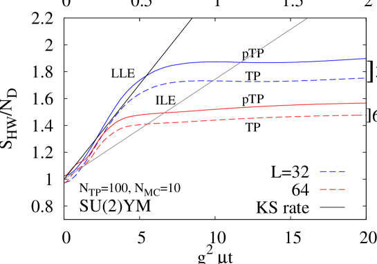
Figure 1: The time evolution of HW entropy by TP and pTP methods in the SU(2) Yang-Mills (YM) lattice field theory on the $32^{3}$ and $64^{3}$ lattices. The horizontal axis shows the time, where the lower (upper) scale is the dimensionless time $g^{2}\mu t$ (the physical time $t_{\mathrm{phys}}$ [fm/c]). The vertical axis is the HW entropy per DOF, $S_{\mathrm{HW}}^{\mathrm{(PA)}}/N_{D}$. The upper (lower) two lines are results on the $32^{3}$ ($64^{3}$) lattice. In the both lattice results, the upper solid (lower dotted) line is the result in the pTP (TP) method. The black (gray) straight line, “KS rate”, is the entropy production rate given by the sum of the positive LLE (ILE) given in Appendix B.

The growth rate of the HW entropy in the linearly increasing stage may be characterised by the Kolmogorov-Sinaï (KS) rate, which is the sum of positive Lyapunov exponents and reflects the underlying dynamics. Due to the scale invariance of classical Yang-Mills, the KS rate scales as $\lambda_{\rm KS}/L^{3}=c_{\rm KS}\times\varepsilon^{1/4}$ kunihiro , where $\varepsilon=\langle H\rangle/L^{3}$ is the energy density. Then the HW entropy is expected to increase as

$$\frac{{S_{\mathrm{HW}}}(t)}{{N_{\mathrm{D}}}}=\frac{{S_{\mathrm{HW}}}(t=0)}{{N_{\mathrm{D}}}}+\frac{\lambda_{\rm KS}}{{N_{\mathrm{D}}}}\,t=1+\frac{c_{\rm KS}}{3(N^{2}_{\rm c}-1)}\,\frac{\varepsilon^{1/4}}{g^{2}\mu}\times g^{2}\mu t.$$ (30)

We consider two types of the KS rate, the local and intermediate KS rates, $\lambda^{\rm LLE}_{\rm KS}$ and $\lambda^{\rm ILE}_{\rm KS}$, obtained from the local and intermediate Lyapunov exponents, LLE and ILE, defined locally in time and in an intermediate time period, respectively kunihiro . For the SU(2) Yang-Mills theory, the coefficient is obtained as $c^{\rm LLE(ILE)}_{\rm KS}\simeq 1.9(1.0)$ by fitting to the data as shown in Appendix B.

In the case of random initial condition discussed in Appendix B, the growth rate in the early time is characterized well by the local KS rate, $\lambda_{\rm KS}^{\rm LLE}$. On the other hand, the entropy growth rate in the intermediate time toward the saturation agrees with the intermediate KS rate, $\lambda_{\rm KS}^{\rm ILE}$. While the local KS rate obtained from the second derivative of the Hamiltonian at initial time is sensitive to the gluon-field configuration itself, the intermediate KS rate represents the intrinsic property of the chaotic system that dose not depend on initial conditions.

In Fig. 1, we compare the numerically obtained HW entropy and that expected from the KS rates. The black straight lines in Fig. 1 show the entropy increase expected from the local and intermediate KS rates. In the present calculation on the $64^{3}$ lattice, the total energy (energy density) amounts to $\langle{H}\rangle=6.5\times 10^{5}$ ($\varepsilon=2.48$), then the slope from the local (intermediate) KS rates, $\frac{c^{\rm LLE(ILE)}_{\rm KS}}{3(N^{2}_{\rm c}-1)}\,\frac{\varepsilon^{1/4}}{g^{2}\mu}$, is evaluated to be $0.14(0.074)$. As seen in Fig. 1, the growth rate of the HW entropy in the early time is around $d{S_{\mathrm{HW}}}/d(g^{2}\mu t)/{N_{\mathrm{D}}}\simeq 0.14$, which is close to the local KS rate and significantly larger than the intermediate KS rate. This comparison implies that we cannot explain the entropy production from the MV model initial condition only by intrinsic chaoticity, and that some instability may be the trigger of the entropy production. In fact, the initial field configuration of the MV model has strong instabilities and the HW entropy is considered to saturate even without showing the intermediate KS rate.

The HW entropy production rate per degrees of freedom in the early stage is almost independent of the lattice size. In addition to $32^{3}$ and $64^{3}$ lattices shown in Fig. 1, similar production rate is found on smaller lattices, $4^{3}$, $8^{3}$ and $16^{3}$. At least, this lattice-size independence dose not come from the chaoticity of the system because the KS rates depend on the lattice size. The energy density on the $32^{3}$ lattice is $\varepsilon=3.53$, and the slopes from the local and intermediate KS rates are evaluated as $0.08$ and $0.04$, respectively, which are smaller than the KS rates on the $64^{3}$ lattice. This fact suggests that another possible mechanism exists to create the HW entropy such as the initial instability.

The amount of the produced entropy on the $64^{3}$ lattice is $\Delta S/N_{D}\simeq 0.4$ and may be in the same order of the expected entropy production. The longitudinal thickness of glasma at the initial stage should be in the order of $Q_{s}^{-1}$, and the present calculation in the nonexpanding geometry corresponds to a very thick nuclei, $aL=120\,Q_{s}^{-1}$. The produced entropy per unit rapidity for color SU(3) is expected to be

$$\frac{\Delta S_{\mathrm{HW}}}{120\Delta Y}=\frac{0.4\times 3(N_{c}^{2}-1)L^{3}}{1200}\simeq 2000\ .$$ (31)

This value is around half of the expected entropy, $\Delta S/\Delta Y\simeq 4500$ EntropyReview , but several systematic uncertainties in the present setup could easily account for a factor of two. Calculation of the entropy production in an expanding geometry is desired.

4.2 Classical equilibration

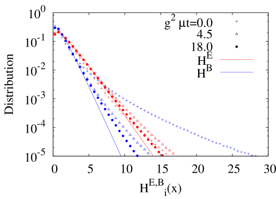
Figure 2: Electric and magnetic local energy distribution in the SU(2) Yang-Mills theory on the $64^{3}$ lattice. The red (blue) crosses, triangles and circles show the electric (magnetic) energy distributions at $g^{2}\mu t=0,4.5$ and $18$, respectively. The red (blue) line shows a fit function $\sqrt{H^{E(B)}}\exp(-H^{E(B)}/T)$ to the electric (magnetic) energy distribution at $g^{2}\mu t=18$.

The present calculation shows that the HW entropy approximately saturates at $g^{2}\mu t\simeq 7(5)$ on the $32^{3}$ $(64^{3})$ lattice, then some kind of quasi-stationary state is formed. In Fig. 2, we show the distribution of the electric and magnetic local energies,

$$H^{E}_{i}(\mathbb{x})=\frac{1}{2}\sum_{a=1}^{N_{c}^{2}-1}\left(E^{a}_{i}(\mathbb{x})\right)^{2}\ ,\quad H^{B}_{i}(\mathbb{x})=\frac{1}{2}\sum_{a=1}^{N_{c}^{2}-1}\left(B^{a}_{i}(\mathbb{x})\right)^{2}\quad(i=x,y,z)\ .$$ (32)

In the thermal equilibrium in the classical regime, the distribution of $(A,E)$ would be described by the Boltzmann distribution,

$$\mathcal{Z}=\int D\Gamma\,\exp(-H/T)=\prod_{i,\mathbb{x}}\left[\int\frac{d^{3}E_{i}(\mathbb{x})}{2\pi\hbar g^{2}}\ e^{-H^{E}_{i}(\mathbb{x})/T}\right]\int DA\ e^{-\sum_{i,\mathbb{x}}H^{B}_{i}(\mathbb{x})/T}\ .$$ (33)

For the electric energy distribution, we can rewrite the measure as $d^{3}E=\sqrt{H^{E}}\,dH^{E}\,d\Omega$ with $d\Omega$ being the solid angle in the color space, and the distribution function can be given as $\sqrt{H^{E}}\exp(-H^{E}/T)$. Actually, the electric energy distribution in the later stage is described well by this distribution except for the high energy region as shown by the solid line in Fig. 2. The magnetic energy distribution is also found to follow the same function but with a different temperature. Similar Boltzmann distribution of the energy is found in Ref. Biro1993 . Thus the saturation of the HW entropy seems to be related to the quasi-statinary state, where approximate equilibrium is reached among the electric energies and among the magnetic energies but with a different temperature.

The saturation time and saturated value of the HW entropy per DOF decrease with increasing lattice size, as shown in Fig. 1. It should be noted that the above quasi-statinary state is, however, different from the true equilibrium of gluons: In addition that the electric and magnetic temperatures are different, the long-term evolution with the classical Yang-Mills equation does not reach the Bose-Einstein distribution of the high-momentum modes but reach the classical statistical distribution. Since the classical statistical distribution in field theories does not have a well-defined continuum limit, it is reasonable to find the lattice size dependence of the saturation time and saturated value of the HW entropy.

4.3 Isotropization of pressure

In Fig. 3, we show the time evolution of the ratio of the pressure to the energy density ratio in the longitudinal and transverse directions, $P_{L,T}/\varepsilon$, on the $16^{3}$, $32^{3}$ and $64^{3}$ lattices. Because the energy-momentum tensor is traceless, the relation $2P_{L}/\varepsilon+P_{T}/\varepsilon=1$ is satisfied. While the classical configuration of the MV model has the completely anisotropic pressure $P_{L}=-P_{T}$ at initial time, the quantum fluctuations modifies this relation and the initial value $P_{L}/\varepsilon$ ($P_{T}/\varepsilon$) is not equal to $1.0$ ($-1.0$).

The isotropization of the pressure can be found to occur in Fig. 3. The lattice size dependence of the isotropization time is strong in the smaller lattices, $L<32$, and For larger lattices $(L\geq 32)$, the isotropization time almost converges $g^{2}\mu t\simeq 10$, as seen from the $L=32$ and $L=64$ results, This isotropization time roughly agrees with the time of the HW entropy saturation. It also happens to agree with the isotropization time obtained in the expanding geometry with fluctuation effects from the finite coupling Epelbaum13 .

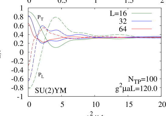
Figure 3: Time evolution of the pressure in the SU(2) Yang-Mills (YM) theory. The horizontal axis is the time axis. The lower (upper) scale is the dimensionless time scale $g^{2}\mu t$ (the physical time $t_{\mathrm{phys}}$ [fm/c]). The vertical axis is the longitudinal and transversal pressure normalized by the energy density, $P_{L,T}/\varepsilon$. The dotted (solid) lines are the longitudinal pressure. The green, blue and red lines corresponds to the results on the $16^{3}$, $32^{3}$ and $64^{3}$ lattices respectively.

5 Summary and conclusion

The aim of this paper is to understand the thermalization in the relativistic heavy ion collisions by focusing on the entropy production. We calculate the Husimi-Wherl (HW) entropy in the Yang-Mills field theory with the phenomenological initial condition given by the McLerran-Venugopalan (MV) model but in the non-expanding geometry. The HW entropy constructed from the Husimi function plays an important role in thermodynamics of quantum systems and its production implies the thermalization of the system.

We calculate the semiclassical time evolution of the Wigner function by solving the classical equation of motion which keeps the gauge invariance of the HW entropy. In actual calculations, we use the product ansatz to reduce the numerical cost at the cost of breaking the gauge invariance of the HW entropy. Nevertheless the HW entropy in the product ansatz agrees with the result without the product ansatz within 10-20% in a few-dimensional quantum mechanical system Tsukiji2016 and production rate of the HW entropy in the product ansatz agrees with the Kolmogolov-Sinaï (KS) rate.

We have found that the HW entropy increases linearly in early time and saturates at later times. The growth rate of the HW entropy is independent of the lattice size and is significantly larger than the intermediate KS rate, defined as the sum of the positive intermediate Lyapunov exponents. This implies that we cannot explain the entropy production from MV initial condition only by intrinsic chaoticity. It also suggests that the large amount of the entropy may be produced by the initial instability. When the HW entropy saturates, the electric and magnetic local energy distributions reach the classical statistical equilibrium except for the high energy regions. The saturation time agrees with the equilibrium time of the local energy distribution and the isotropization time of the pressure, which suggests the thermalization of the gluon field is realized in the sense of the HW entropy production. The saturation time is around $1$ fm/c. In order to reach more quantitative and realistic conclusions, the evaluation the HW entropy in the expanding geometry is desired, which is under progress.

Appendix A Gauge invariance of Husimi-Wehrl entropy

We give proof of the invariance of Husimi-Wehrl entropy with the residual gauge freedom in temporal gauge.

A.1 Gauge invariance of Wigner function

In temporal gauge ($A_{0}=0$), the gauge transformation is given by

$$A_{i} \to A^{\prime}_{i}=\Omega A_{i}\Omega^{-1}+i\Omega\partial_{i}\Omega^{-1},$$

$$E_{i} \to E^{\prime}_{i}=\Omega E_{i}\Omega^{-1}.$$ (34)

A vector in Hilbert space is transformed by

$$|A\rangle\to|A^{\prime}\rangle=\hat{\Omega}|A\rangle=|\Omega A\Omega^{-1}+i\Omega\partial\Omega^{-1}\rangle.$$ (35)

When the density matrix $\rho$ is gauge covariant;

$$\rho\to\hat{\rho}^{\prime}=\hat{\Omega}\hat{\rho}\hat{\Omega}^{-1},$$ (36)

we can prove the gauge invariance of the Wigner function.

The Wigner function is transformed by

$$f_{\scriptscriptstyle{W}}[A,E]\to f_{\scriptscriptstyle{W}}[A^{\prime},E^{\prime}]$$

$$= \int\frac{Da}{(2\pi\hbar g^{2})^{{N_{\mathrm{D}}}}}\mathrm{e}^{iE^{\prime}\cdot a/\hbar g^{2}}\langle A^{\prime}+a/2|\hat{\rho}^{\prime}|A^{\prime}-a/2\rangle$$

$$= \int\frac{Da^{\prime}}{(2\pi\hbar g^{2})^{{N_{\mathrm{D}}}}}\mathrm{e}^{iE^{\prime}\cdot a^{\prime}/\hbar g^{2}}\langle A^{\prime}+a^{\prime}/2|\hat{\rho}^{\prime}|A^{\prime}-a^{\prime}/2\rangle$$

$$= \int\frac{Da^{\prime}}{(2\pi\hbar g^{2})^{{N_{\mathrm{D}}}}}\mathrm{e}^{iE^{\prime}\cdot(a^{\prime}-i\Omega\partial\Omega^{-1})/\hbar g^{2}}\langle A^{\prime}+\frac{a^{\prime}}{2}-\frac{i}{2}\Omega\partial\Omega^{-1}|\hat{\rho}^{\prime}|A^{\prime}-\frac{a^{\prime}}{2}+\frac{i}{2}\Omega\partial\Omega^{-1}\rangle$$

$$= \int\frac{Da}{(2\pi\hbar g^{2})^{{N_{\mathrm{D}}}}}\mathrm{e}^{i\Omega E\Omega^{-1}\cdot\Omega a\Omega^{-1}/\hbar g^{2}}\langle A+\frac{a}{2}|\hat{\Omega}^{\dagger}\Omega\hat{\rho}\Omega^{-1}\Omega|A-\frac{a}{2}\rangle$$

$$= f_{\scriptscriptstyle{W}}[A,E].$$ (37)

We use the transformation of the $|A\pm a/2\rangle$,

$$|A\pm a/2\rangle\to\hat{\Omega}|A\pm a/2\rangle = |\Omega A\Omega^{-1}\pm\Omega a\Omega^{-1}/2+i\Omega\partial\Omega^{-1}\rangle$$ (38)

$$= |A^{\prime}\pm a^{\prime}/2\mp i\Omega\partial\Omega^{-1}/2\rangle.$$

The equation (37) shows the gauge invariance of the Wigner function.

A.2 Gauge invariance of Husimi function and Husimi-Wehrl entropy

It is easy to prove the gauge invariance of the Husimi function from the above discussion.

The gauge transformation of the Husimi function is given by

$$f_{\scriptscriptstyle{H}}[A,E]\to f_{\scriptscriptstyle{H}}[A^{\prime},E^{\prime}]$$

$$= \int\frac{D\bar{A}D\bar{E}}{(\pi\hbar g^{2})^{{N_{\mathrm{D}}}}}\mathrm{e}^{-\Delta(A^{\prime}-\bar{A})^{2}/\hbar-(E^{\prime}-\bar{E})^{2}/\Delta\hbar g^{2}}f_{\scriptscriptstyle{W}}[\bar{A},\bar{E}]$$

$$= \int\frac{D\bar{A^{\prime}}D\bar{E^{\prime}}}{(\pi\hbar g^{2})^{{N_{\mathrm{D}}}}}\mathrm{e}^{-\Delta(A^{\prime}-\bar{A}^{\prime})^{2}/\hbar g^{2}-(E^{\prime}-\bar{E}^{\prime})^{2}/\Delta\hbar g^{2}}f_{\scriptscriptstyle{W}}[\bar{A}^{\prime},\bar{E}^{\prime}]$$

$$= \int\frac{D\bar{A}D\bar{E}}{(\pi\hbar g^{2})^{{N_{\mathrm{D}}}}}\mathrm{e}^{-\Delta(\Omega A\Omega^{-1}-\Omega\bar{A}\Omega^{-1})^{2}/\hbar g^{2}-(\Omega E\Omega^{-1}-\Omega\bar{E}\Omega^{-1})^{2}/\Delta\hbar g^{2}}f_{\scriptscriptstyle{W}}[\bar{A},\bar{E}]$$

$$= f_{\scriptscriptstyle{H}}[A,E].$$ (39)

This equation show the gauge invariance of Husimi function. The gauge invariance of Husimi-Wehrl entropy follows from these facts.

A.3 Gauge invariance in semiclassical approximation

In this subsection, we prove that the semiclassical time evolution dose not break the gauge invariance of the HW entropy.

When the Wigner function is gauge invariant at initial time, it is gauge invariant at any time in semiclassical approximation.

$$f_{\scriptscriptstyle{W}}[A,E;t]\to f_{\scriptscriptstyle{W}}[A^{\prime},E^{\prime};t]$$

$$= f_{\scriptscriptstyle{W}}[A^{\prime},E^{\prime};t=0]$$

$$= f_{\scriptscriptstyle{W}}[A,E;t=0]=f_{\scriptscriptstyle{W}}[A,E;t]$$ (40)

Because the classical path is gauge covariant, the $(A^{\prime},E^{\prime};t)$ at time $t$ and $t=0$ are on the same gauge orbit.

Therefore, the semiclassical time evolution keeps the gauge invariant of the HW entropy.

Appendix B Lyapunov exponents in SU(2) Yang-Mills theory

In this Appendix, we show the calculated results of the Lyapunov exponents in the SU(2) Yang-Mills theory and show that the Lyapunov exponents are proportional to $\varepsilon^{1/4}$, where $\varepsilon$ is the energy density. Results for the SU(3) Yang-Mills theory is given in Ref. kunihiro . Our numerical formalism and set-up are the same as that of Ref. kunihiro . To detect the intrinsic property of the system such as chaoticity, we set the initial condition as $E=0$ and $A$ is randomly chosen around zero.

B.1 Results

We summarize our results in Table 1 and Fig. 4. Our results show the Lyapunov exponents are proportional to the $\varepsilon^{1/4}$ and we determine the coefficients by fitting the results;

$$\lambda^{\rm LLE}_{\rm max} = c^{\rm LLE}_{\rm max}\times\varepsilon^{1/4}=1.3\times\varepsilon^{1/4},$$ (41)

$$\lambda^{\rm LLE}_{\rm KS}/L^{3} = c^{\rm LLE}_{\rm KS}\times\varepsilon^{1/4}=1.9\times\varepsilon^{1/4},$$ (42)

$$\lambda^{\rm ILE}_{\rm max} = c^{\rm ILE}_{\rm max}\times\varepsilon^{1/4}=0.3\times\varepsilon^{1/4},$$ (43)

$$\lambda^{\rm ILE}_{\rm KS}/L^{3} = c^{\rm ILE}_{\rm KS}\times\varepsilon^{1/4}=1.0\times\varepsilon^{1/4}.$$ (44)

Table 1: Lyapunov exponents in SU(2) classical Yang-Mills theory

$L^{3}$	$\varepsilon$	$\lambda^{\rm LLE}_{\rm max}$	$\lambda^{\rm LLE}_{\rm KS}$	$\lambda^{\rm ILE}_{\rm max}$	$\lambda^{\rm ILE}_{\rm KS}$
$4^{3}$	0.054	0.569	38.1	0.137	15.9
$4^{3}$	0.38	0.938	66.0	0.196	42.7
$4^{3}$	2.14	1.48	124	0.339	78.2
$4^{3}$	7.17	2.07	254	0.616	112
$4^{3}$	18.6	2.73	254	0.616	139
$4^{3}$	79.9	4.14	383	0.939	189

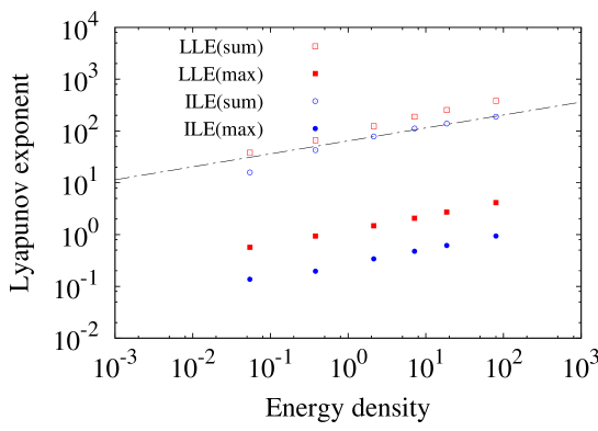
Figure 4: Lyapunov exponents in the SU(2) Yang-Mills lattice field theory with random initial condition, $\lambda^{\rm LLE}_{\rm max},\lambda^{\rm LLE}_{\rm KS},\lambda^{\rm ILE}_{\rm max},\lambda^{\rm ILE}_{\rm KS}$. The blocken line is $4^{3}\times\varepsilon^{1/4}$.

B.2 Comparison with Husimi-Wherl entropy

We reexamine the result in the Ref. Tsukiji2016 with the Lyapunov exponents in SU(2) Yang-Mills theory. Fig. 5 shows the time evolution of the HW entropy in SU(2) Yang-Mills theory with the Gaussian random initial condition around the origin. The black (gray) straight line shows the HW entropy with the growth rate given by the local (intermediate) KS rate defined as the sum of positive LLE (ILE). The growth rate caused by instabilities in the early time is characterized by the local KS rate and the entropy growth rate in the intermediate time caused by chaoticity, which is the intrinsic property of the Yang-Mills system, is characterized by the intermediate KS rate.

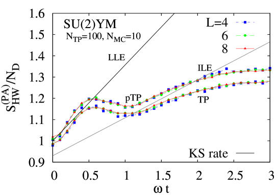
Figure 5: The time evolution of HW entropy by TP and pTP methods in the SU(2) Yang-Mills (YM) lattice field theory with random initial condition. The blue squre, green circle and red triangle lines are the HW entropy per one degree of freedom on $4^{3},6^{3}$ and $8^{3}$ lattices, respectively. The black (gray) solid line shows the growth rate of local (intermediate) KS rate.

References

- (1) I. Arsene et al. [BRAHMS Collaboration], Nucl. Phys. A 757, 1 (2005).
- (2) K. Adcox et al. [PHENIX Collaboration], Nucl. Phys. A 757, 184 (2005).
- (3) B. B. Back et al. [PHOBOS Collaboration], J. Phys. G 31, S41 (2005).
- (4) J. Adams et al. [STAR Collaboration], Nucl. Phys. A 757, 102 (2005).
- (5) B. Muller, J. Schukraft, and B. Wyslouch, Annu. Rev. Nucl. Part. Sci. 62, 361 (2012).
- (6) P. F. Kolb and U. W. Heinz, In *Hwa, R.C. (ed.) et al.: Quark gluon plasma* 634-714.
- (7) M. Gyulassy and L. McLerran, Nucl. Phys. A 750, 30 (2005).
- (8) U. Heinz and P. Kolb, Nucl. Phys. A702 269 (2002).
- (9) R. Baier, A.H. Mueller, D. Schiff, and D.T. Son, Phys. Lett. B 502, 51 (2001).
- (10) R. Baier, A.H. Mueller, D. Schiff, and D.T. Son, Phys. Lett. B 539, 46 (2002).
- (11) T. Lappi and L. McLerran, Nucl. Phys. A772 220 (2006).
- (12) P. Arnold, J. Lenaghan, G. D. Moore, and L. G. Yaffe, Phys. Rev. Lett. 94, 072302 (2005).
- (13) P. Romatschke and R. Venugopalan, Phys. Rev. Lett. 96, 062302 (2006).
- (14) P. Romatschke and R.Venugopalan, Phys. Rev. D74, 045011 (2006).
- (15) J. Berges, S. Scheffler, and D. Sexty, Phys. Rev. D 77, 034504 (2008).
- (16) J. Berges, D. Gelfand, S. Scheffler, D Sexty, Phys. Lett. B 677, 210 (2009).
- (17) K. Fukushima and F.Gelis, Nucl. Phys. A874, 108-129 (2012).
- (18) J. Berges, S. Scheffler, S. Schlichting, and D. Sexty, Phys. Rev. D 85, 034507 (2012).
- (19) S. Tsutsui, H. Iida, T. Kunihiro, and A. Ohnishi, Phys. Rev. D 91, 076003 (2015).
- (20) S. Tsutsui, T. Kunihiro and A. Ohnishi, Phys. Rev. D 94, 016001 (2016).
- (21) T. Epelbaum and F. Gelis, Phys. Rev. Lett. 111, 232301 (2013); Nucl. Phys. A926, 122 (2014).
- (22) M. Ruggieri, F. Scardina, S. Plumari, and V. Greco, Phys. Rev. C 89, 054914 (2014).
- (23) M. Ruggieri, A. Puglisi, L. Oliva, S. Plumari, F. Scardina, and V. Greco, Phys. Rev. C 92, 064904 (2015).
- (24) A. Kurkela and Y. Zhu, Phys. Rev. Lett. 115, 182301 (2015).
- (25) B. Muller and A. Schafer, Int. J. Mod. Phys. E 20, 2235 (2011).
- (26) H. Taya, Phys. Rev. D 96, no. 1, 014033 (2017).
- (27) J. Berges, K. Reygers, N. Tanji and R. Venugopalan, Phys. Rev. C 95, no. 5, 054904 (2017).
- (28) B. Muller and A. Trayanov, Phys. Rev. Lett. 68, 3387 (1992).
- (29) T. S. Biro, C. Gong, B. Muller and A. Trayanov, Int. J. Mod. Phys. C 5, 113 (1994).
- (30) T. Kunihiro, B. Müller, A. Ohnishi, A. Schäfer, T.T. Takahashi and A. Yamamoto, Phys. Rev. D82, 114015 (2010).
- (31) H. Iida, T. Kunihiro, B. Muller, A. Ohnishi, A. Schafer, and T.T. Takahashi, Phys. Rev. D 88, 094006 (2013).
- (32) H. Tsukiji, H. Iida, T. Kunihiro, A. Ohnishi, and T. T. Takahashi, Prog. Theor. Exp. Phys. 083A01 (2015).
- (33) H. Tsukiji, H. Iida, T. Kunihiro, A. Ohnishi, and T. T. Takahashi, Phys. Rev. D 94, 091502(R) (2016).
- (34) A. Wehrl, Rev. Mod. Phys. 50, 221 (1978).
- (35) A. Wehrl, Rep. Math. Phys. 16, 353 (1979).
- (36) E.P. Wigner, Phys. Rev. 40, 749 (1932).
- (37) M. Hillery, R. F. O’Connell, M. O. Scully and E. P. Wigner, Phys. Rept. 106, 121 (1984).
- (38) S. Mrowczynski and B. Muller, Phys. Rev. D 50, 7542 (1994).
- (39) K. Fukushima, F. Gelis and L. McLerran, Nucl. Phys. A 786, 107 (2007).
- (40) H. Weyl, The Theory of Groups and Quantum Mechanics, (Dover, N.Y., 1931).
- (41) K. Husimi, Proc. Phys. Math. Soc. Jpn. 22, 123 (1940).
- (42) K. Takahashi, J. Phys. Soc. Jpn. 55, 762 (1986).
- (43) K. Takahashi, Prog. Theor. Phys. Suppl. 98, 109 (1989).
- (44) T. Kunihiro, B. Müller, A. Ohnishi, and A. Schafer, Prog. Theor. Phys. 121, 555 (2009).
- (45) L. McLerran and R. Venugopalan, Phys. Rev. D49, 2233 (1994); ibid. 49 3552 (1994); ibid. 50, 2225 (1994).
- (46) A. Kovner, L. McLerran, and H. Weigert, Phys. Rev. D 52, 3809 (1995).
- (47) H. Iida, T. Kunihiro, A. Ohnishi, and T. T. Takahashi, arXiv: 1410.7309.
- (48) A good review is A. Polkovnikov, Annals Phys. 325, 1790 (2010).
- (49) E. H. Lieb, Commun. Math. Phys. 62 (1978) 35.