Bisimulation and Hennessy-Milner Logic for Generalized Synchronization Trees

Abstract

In this work, we develop a generalization of Hennessy-Milner Logic (HML) for Generalized Synchronization Trees (GSTs) that we call Generalized Hennessy Milner Logic (GHML). Importantly, this logic suggests a strong relationship between (weak) bisimulation for GSTs and ordinary bisimulation for Synchronization Trees (STs). We demonstrate that this relationship can be used to define the GST analog for image-finiteness of STs. Furthermore, we demonstrate that certain maximal Hennessy-Milner classes of STs have counterparts in maximal Hennessy-Milner classes of GSTs with respect to GST weak bisimulation. We also exhibit some interesting characteristics of these maximal Hennessy-Milner classes of GSTs.

1 Introduction

In the context of discrete systems modeled as Synchronization Trees (STs), Hennessy and Milner first noticed a relationship between bisimulation and a simple modal logic, subsequently to be known as Hennessy-Milner logic (HML) [14]. In particular, they observed that HML characterizes bisimulation within the class of image-finite STs in the following sense: two image-finite STs are bisimilar if and only if they satisfy exactly the same HML formulas. Subsequent to Hennessy and Milner’s original work, HML has likewise been shown to characterize bisimulation within other classes of STs (though not the class of all STs [17]). Indeed, any class of STs for which modal equivalence implies bisimulation is known as a Hennessy-Milner class (HM class), and a number of maximal ones have been exhibited [15].

Such characterizations of bisimulation have significant ramifications for the verification of system properties: if two systems belong to the same HM class, then they can be checked for bisimulation equivalence by checking HML formulas instead. In addition, if two such systems are not bisimilar, then an HML formula can bear witness to this lack of bisimilarity [3]. For a simple logic such as HML, this is a considerable advantage. Moreover, the existence of maximal HM classes is particularly important in the study of STs and process algebra, given the inherent compositionality of those objects. In particular, it is useful to know which operations preserve membership in a maximal HM class; this has been considered for some cases in [15].

Recently, the authors have proposed Generalized Synchronization Trees (GSTs) [10] as a flexible modeling framework for non-discrete systems such as continuous or hybrid systems. Despite their broader applicability, GSTs have many similarities to STs: elegant composition operators between GSTs are plentiful, and there are well defined notions of bisimulation (see [10]). Thus, GSTs are natural candidates for the treatment of both HML-like logics and HM classes, especially with a view to studying the composition of continuous and hybrid systems. This paper launches such a study and makes three crucial contributions on the topic of modal logic for non-discrete systems: first, we define a novel generalization of HML that has semantic parity with trajectories in GSTs; second, we use this logic to define a notion of image finiteness for GSTs; and third, we exhibit a partial characterization of maximal HM classes in the context of our generalized HML. The third contribution is particularly novel, since there seem to be no results at all about maximal HM classes for generic hybrid system models, much less results in a framework as flexible and compositional as GSTs. Since GSTs can exhibit infinite – and even continuous – non-determinism, they offer a particularly rich setting in which to explore the structure of HM classes.

There are other results in the hybrid systems literature that relate bisimulation to modal logics (see e.g. [5]), but these results typically focus on establishing that bisimulation preserves the satisfaction of formulas from some modal logic. Almost none consider the problem of specifying when modal equivalence implies bisimilarity, i.e. the identification of Hennessy-Milner classes. The few papers that do consider the problem of identifying HM classes seem to be concerned with probabilistic systems: see [6, 7, 8, 18, 9, 4, 2] for example. However, in most of these papers, the following quote is emblematic of the source of these results: “… the probabilistic systems we are considering, without explicit nondeterminism, resemble deterministic systems quite closely, rather than nondeterministic systems” [6]. In other words, these papers typically end up with something like an image-finite assumption, and that forms the basis of their HM classes. On the other hand, the papers that do not have an image-finiteness assumption ([18, 9]) always consider more complicated logics than HML, and do not address questions of maximal HM classes.

2 Background

This section describes several foundational results that will be used subsequently. The first subsection contains background material on GSTs, including a review of the relevant notions of bisimulation for the same. The second subsection contains background material on HML and Hennessy and Milner’s result for image-finite processes. The third subsection describes some maximal Hennessy-Milner classes over Kripke structures [15] and some necessary preliminaries on the canonical model [11]. Table 1 describes some common notation that will be used throughout this section and the rest of the paper.

$Sys_{1}\;\overset{\rightarrow}{\rule{5.8pt}{0.5pt}}_{X}\;Sys_{2}$	:	$Sys_{2}$ simulates $Sys_{1}$ (w.r.t. simulation notion $X$)
$Sys_{1}\;\overset{\leftrightarrow}{\rule{5.8pt}{0.5pt}}_{X}\;Sys_{2}$	:	$Sys_{1}$ and $Sys_{2}$ are bisimilar (w.r.t. simulation notion $X$)
$s\;\overset{\leftrightarrow}{\rule{5.8pt}{0.5pt}}_{X}\;t$	:	States (or worlds, nodes) $s$ and $t$ are bisimilar (w.r.t. simulation notion $X$)
$Sys_{1}\;\approx_{Y}\;Sys_{2}$	:	$Sys_{1}$ and $Sys_{2}$ satisfy the same formulas of logic $Y$
$s\;\approx_{Y}\;t$	:	States (or worlds, nodes) $s$ and $t$ satisfy the same formulas of logic $Y$

Table 1: Notation for simulation, bisimulation and modal equivalence.

2.1 Generalized Synchronization Trees

This section summarizes the theory of GSTs as presented in [10]; the interested reader is referred to that reference for more details.

GSTs extend Milner’s Synchronization Trees (STs) via a generalized notion of tree. In particular, the essential element of a GST is the tree partial order, a well known structure in the mathematical literature (see [16], for example).

Definition 1 (Tree [16, 10]).

A tree is a triple $\langle P,\preceq,p_{0}\rangle$, where $\langle P,\preceq\rangle$ is a partial order, $p_{0}\in P$, and the following hold.

1. $p_{0}\preceq p$ for all $p\in P$ ($p_{0}$ is called the root of the tree)

2. For any $p\in P$ the set $[p_{0},p]\triangleq\{p^{\prime}\in P:p_{0}\preceq p^{\prime}\preceq p\}$ is totally ordered by $\preceq$.

In this definition of a tree, there is no inherent notion of edge, or “discrete” transition, so unlike STs external interactivity cannot be captured by labeling edges; such action labels need a different encoding. The definition of GSTs below suggests just such a scheme.

Definition 2 (Generalized Synchronization Tree [10]).

Let $L$ be a set of labels. Then a Generalized Synchronization Tree (GST) is a tuple $\langle P,\preceq,p_{0},\mathcal{L}\rangle$, where:

1. $\langle P,\preceq,p_{0}\rangle$ is a tree in the sense of Definition 1; and

2. $\mathcal{L}\in P\backslash\{p_{0}\}\rightarrow L$ is the labeling function (may be partial).

Intuitively, labels in a GST are affixed to nodes in the tree. If the tree is discrete, it can be converted into an ST by moving the node labels onto the incoming edge from the nodes parent (note that roots are not labeled in GSTs, so this operation is well-defined).

Another consequence of a lack of discrete transitions is that bisimulation must be defined differently than for STs. Specifically, bisimulation between GSTs is defined in trajectories, which are totally ordered sets of nodes in a GST that play roughly the same role as transitions (or sequences of transitions) in discrete bisimulation.

Definition 3 (Trajectory [10]).

Let $\langle P,\preceq,p_{0},\mathcal{L}\rangle$ be a GST, and let $p\in P$. Then a trajectory from $p$ is either:

1. the set $(p,p^{\prime}]\triangleq\{p^{\prime\prime}\in P:p\prec p^{\prime\prime}\preceq p^{\prime}\}$ for some $p^{\prime}\succ p$, or

2. a (set-theoretic) maximal linear subset $P^{\prime}\subseteq P$ with the property that for all $p^{\prime}\in P^{\prime}$, $p^{\prime}\succ p$.

Trajectories of the first type are called bounded, while those of the second type are called (potentially) unbounded.

To account for the labels on the nodes of a trajectory, we define a notion of order equivalence to parallel the notion of identically labeled transitions in a ST:

Definition 4 (Order Equivalence [10]).

Let $\langle P,\preceq_{P},p_{0},\mathcal{L}_{P}\rangle$ and $\langle Q,\preceq_{Q},q_{0},\mathcal{L}_{Q}\rangle$ be GSTs, let $T_{p},T_{q}$ be trajectories from $p\in P$ and $q\in Q$ respectively. Then $T_{p}$ and $T_{q}$ are order-equivalent if there exists a bijection $\lambda\in T_{P}\rightarrow T_{Q}$ such that:

1. $p_{1}\preceq_{P}p_{2}$ if and only if $\lambda(p_{1})\preceq_{Q}\lambda(p_{2})$ for all $p_{1},p_{2}\in T_{P}$, and

2. $\mathcal{L}_{P}(p)=\mathcal{L}_{Q}(\lambda(p))$ for all $p\in T_{P}$

When $\lambda$ has this property, we say that $\lambda$ is an order equivalence from $T_{P}$ to $T_{Q}$.

We now recall the two notions of simulation from [10]; corresponding notions of bisimulation can be defined in the obvious way [10].

Definition 5 (Weak Simulation for GSTs [10]).

Let $G_{1}=\langle P,\preceq_{P},p_{0},\mathcal{L}_{P}\rangle$ and $G_{2}=\langle Q,\preceq_{Q},q_{0},\mathcal{L}_{Q}\rangle$ be GSTs. Then $R\subseteq P\times Q$ is a weak simulation from $G_{1}$ to $G_{2}$ if, whenever $\langle p,q\rangle\in R$ and $p^{\prime}\succeq p$, then there is a $q^{\prime}\succeq q$ such that:

1. $\langle p^{\prime},q^{\prime}\rangle\in R$, and

2. Trajectories $(p,p^{\prime}]$ and $(q,q^{\prime}]$ are order-equivalent.

We say $G_{1}\overset{\rightarrow}{\rule{5.8pt}{0.5pt}}_{w}G_{2}$ if there is a weak simulation $R$ from $G_{1}$ to $G_{2}$ with $\langle p_{0},q_{0}\rangle\in R$.

Definition 6 (Strong Simulation for GSTs [10]).

Let $G_{1}=\langle P,\preceq_{P},p_{0},\mathcal{L}_{P}\rangle$ and $G_{2}=\langle Q,\preceq_{Q},q_{0},\mathcal{L}_{Q}\rangle$ be GSTs. Then $R\subseteq P\times Q$ is a strong simulation from $G_{1}$ to $G_{2}$ if, whenever $\langle p,q\rangle\in R$ and $T_{p}$ is a trajectory from $p$, there is a trajectory $T_{q}$ from $q$ and bijection $\lambda\in T_{p}\rightarrow T_{q}$ such that:

1. $\lambda$ is an order equivalence from $T_{p}$ to $T_{q}$, and

2. $\langle p^{\prime},\lambda(p^{\prime})\rangle\in R$ for all $p^{\prime}\in T_{p}$.

We write $G_{1}\overset{\rightarrow}{\rule{5.8pt}{0.5pt}}_{s}G_{2}$ if there is a strong simulation $R$ from $G_{1}$ to $G_{2}$ with $\langle p_{0},q_{0}\rangle\in R$.

2.2 Hennessy-Milner Logic and a Hennessy-Milner Class

2.2.1 Hennessy-Milner Logic

Hennessy-Milner Logic is defined as follows; note the lack of atomic propositions.

Definition 7 (Hennessy-Milner Logic (HML) [14]).

Given a set of labels, $L$, Hennessy-Milner Logic (HML) is the set of formulas $\Phi_{\text{HML}}(L)$ specified as follows, where $\ell\in L$:

$$\varphi:=\top\quad|\quad\neg\varphi\quad|\quad\varphi_{1}\wedge\varphi_{2}\quad|\quad\langle\ell\rangle\varphi.$$ (1)

In [14], the semantics of this logic are defined in following familiar way over STs.

Definition 8 (Semantics of HML [14]).

A satisfaction relation of HML for a set of STs $\mathcal{P}$ is a set $\models\subseteq\mathcal{P}\times\Phi_{\text{HML}}(L)$ such that:

1. $p\models\top$ for all $p\in\mathcal{P}$;

2. $p\models\neg\varphi$ if and only if $p~{}\cancel{\models}~{}\varphi$;

3. $p\models\varphi_{1}\wedge\varphi_{2}$ if and only if $p\models\varphi_{1}$ and $p\models\varphi_{2}$; and

4. $p\models\langle l\rangle\varphi$ if and only if there exists a $p^{\prime}$ such that $p\overset{l}{\rightarrow}p^{\prime}$ and $p^{\prime}\models\varphi$.

Here $p\overset{l}{\rightarrow}p^{\prime}$ means $p^{\prime}$ is a subtree of $p$ whose root is a child of the root of $p$, with the edge connecting the roots labeled by $l$.

Remark 1.

We will freely avail ourselves of usual derived operators such as $\bot$, $\vee$, $\rightarrow$ and $[\ell]$.

2.2.2 Bisimulation and a Hennessy-Milner Class

Hennessy and Milner noticed that STs satisfying the same HML formulas need not be bisimilar; i.e. $p\approx_{\text{HML}}q\;\;\cancel{\Rightarrow}\;\;p\;\overset{\leftrightarrow}{\rule{5.8pt}{0.5pt}}\;q$ in general [14]. Nevertheless, they exhibited a class of STs for which HML modal equivalence does imply bisimilarity: that is the class of image-finite STs.

Definition 9 (Image-Finite Process [14]).

A ST $p\in\mathcal{P}$ is said to be image-finite if for each subtree $q$ of $p$ (including $p$ itself) and each label $\ell\in\mathcal{L}$, the set $\{q^{\prime}:q\overset{\ell}{\rightarrow}q^{\prime}\}$ is finite.

Hennessy and Milner proved the following theorem.

Theorem 1 (Image-Finite Hennessy-Milner Theorem [14]).

Let $p$ and $q$ be any two image-finite STs. Then

$$p\;\overset{\leftrightarrow}{\rule{5.8pt}{0.5pt}}\;q\Longleftrightarrow p\approx_{\text{HML}}q.$$ (2)

Remark 2.

Any theorem with a conclusion of the form (2) is called a Hennessy-Milner Theorem. Likewise, any class of STs (or systems, Kripke structures, etc.) for which a Hennessy-Milner Theorem can be exhibited is called a Hennessy-Milner class.

2.3 The Canonical Model and (Maximal) Hennessy-Milner Classes

Since Hennessy and Milner’s work [14], other Hennessy-Milner classes have been exhibited. In particular, Visser, via Hollenberg [15], has generalized the idea of a Hennessy-Milner class to Kripke structures, and exhibited certain maximal Hennessy-Milner classes of Kripke structures. This section describes the characterization of these classes.

As a prelude, we introduce the following familiar definitions of modal logic, Kripke structure and bisimulation between Kripke structures.

Definition 10 (Modal Logic [11]).

By a modal logic, we mean formulas constructed as in Definition 7 but with the addition of propositional variables (atomic propositions). The set of formulas with a set of propositional variables $\Theta$ and a set of labels $L$ is denoted by $\Phi_{\Theta}(L)$.

Definition 11 (Kripke structure [11, 15]).

A Kripke structure of a set of labels $L$ and a set of propositional variables $\Theta$ is a tuple $\mathbf{S}=(S,\{R_{\ell}\subseteq S\times S:\ell\in L\},V)$ where

• $S$ is the set of states (or worlds);

• for each $\ell\in L$, $R_{\ell}\subseteq S\times S$ is a transition relation for label $\ell$; and

• $V:\Theta\rightarrow 2^{S}$ is a function that maps propositional variables to sets of states.

Definition 12 (Satisfaction relation for a Kripke structure).

Given a Kripke structure $\mathbf{S}=(S,\{R_{\ell}\subseteq S\times S:\ell\in L\},V)$, a satisfaction relation $\models\subseteq S\times\Phi_{\Theta}(L)$ is defined as in Definition 7 with the addition that for any $\theta\in\Theta$, $s\models\theta$ if and only if $s\in V(\theta)$.

Definition 13 (Bisimulation between Kripke structures).

Given two Kripke structures $\mathbf{S}$ and $\mathbf{T}$, we say that $s\in S$ and $t\in T$ are bisimilar or $s\;\overset{\leftrightarrow}{\rule{5.8pt}{0.5pt}}_{K}\;t$ if there is a bisimulation relation $\sim$ such that $s\sim t$, and for all $s^{\prime}\in S,t^{\prime}\in T$, and $\theta\in\Theta$, $s^{\prime}\sim t^{\prime}$ implies $s^{\prime}\models\theta\Leftrightarrow t^{\prime}\models\theta$. Bisimulation between Kripke structures is defined in the obvious way.

2.3.1 The Canonical Model for a Modal Logic

The so-called canonical model – called the Henkin model in [15] – is a special Kripke structure that is one of the most important tools in the study of (normal) modal logic(s). In the canonical model states (or worlds) are defined in terms of the modal formulas that they satisfy. In our context it has an important connection to the maximal Hennessy-Milner classes we will consider; see Subsection 2.3.2. This subsection is meant to be a summary of the relevant material in [11]; the full details can be found therein.

In order to define the canonical model, we must first establish certain consistency criteria that we will enforce on any “reasonable” set of formulas. Any such “reasonable” set of formulas will (somewhat confusingly) be called a logic.

Definition 14 (Logic [11]).

A set of modal formulas $\Lambda\subseteq\Phi_{\Theta}(L)$ is called a logic if it satisfies:

1. $\Lambda$ contains all of the tautologies: that is all of the formulas which are true irrespective of how we assign truth values to modal sub-formulas and propositional variables; and

2. $\Lambda$ is closed under modus ponens: if $\varphi_{1}\in\Lambda$ and $\varphi_{1}\rightarrow\varphi_{2}\in\Lambda$, then $\varphi_{2}\in\Lambda$.

Definition 15 ($\Lambda$-Consistent Set of Modal Formulas [11]).

Given a logic $\Lambda\subseteq\Phi_{\Theta}(L)$, a set of modal formulas $\Gamma\subseteq\Phi_{\Theta}(L)$ is said to be $\Lambda$-consistent if there is no formula of the form $\varphi_{0}\rightarrow(\varphi_{1}\rightarrow(\dots\rightarrow(\varphi_{n}\rightarrow\bot)\dots)$ in $\Lambda$, where $\varphi_{0},\dots,\varphi_{n}\in\Gamma$.

Definition 16 ($\Lambda$-maximal set of formulas [11]).

Given a logic $\Lambda$, a set of formulas $\Gamma\subseteq\Phi_{\Theta}(L)$ is said to be $\Lambda$-maximal if it satisfies the following two properties:

1. $\Gamma$ is $\Lambda$-consistent; and

2. for all $\varphi\in\Phi_{\Theta}(L)$, either $\varphi\in\Gamma$ or $\neg\varphi\in\Gamma$.

Lemma 1 (Lindenbaum’s Lemma [11]).

Given a logic $\Lambda$ and a $\Lambda$-consistent set of formulas $\Gamma$, there exists a $\Lambda$-maximal set of formulas $\Gamma_{0}\subseteq\Phi_{\Theta}(L)$ such that $\Gamma\subseteq\Gamma_{0}$.

Corollary 1 (The set of maximal $\Lambda$-consistent sets of formulas is non-empty [11]).

Given a logic $\Lambda$, let $S^{\Lambda}$ denote the set of $\Lambda$-maximal sets of formulas. Then $S^{\Lambda}$ is non-empty.

For our purposes, Corollary 1 tells us that the set of maximally consistent sets of formulas is non-empty, and hence, can be used as the set of worlds for the canonical model. The next step in the construction of the canonical model is to define the transitions between these states; these must ensure that a state – a $\Lambda$-maximal set of formulas – satisfies a modal formula if an only if that formula is an element of the set. This desirable property – called the “Henkin property” in [15] – is the essence of the value of the canonical model. It turns out that some additional conditions must be imposed on a logic $\Lambda$ before transitions can be defined between $\Lambda$-maximal sets of formulas in such a way that the Henkin property holds.

Definition 17 (Normal Logic [11]).

A logic $\Lambda$ is normal if it satisfies:

1. for all $\varphi_{1},\varphi_{2}\in\Phi_{\Theta}(L)$ and $\ell\in L$, the formula $[\ell](\varphi_{1}\rightarrow\varphi_{2})\rightarrow([\ell]\varphi_{1}\rightarrow[\ell]\varphi_{2})$ is in $\Lambda$;

2. for all $\varphi\in\Lambda$ and $\ell\in L$, $[\ell]\varphi\in\Lambda$.

With this definition in hand, we can define the canonical model.

Definition 18 (Canonical (Henkin) Model [11, 15]).

Let $\Lambda\subseteq\Phi_{\Theta}(L)$ be a normal logic. Then the canonical model is the Kripke structure $\mathbf{C}^{\Lambda}=(S^{\Lambda},\{R_{\ell}^{\Lambda}:\ell\in L\},V^{\Lambda})$ defined as follows:

• $S^{\Lambda}$ is the set of states (worlds);

• for each $\ell\in L$, the transition relation $R_{\ell}^{\Lambda}\subseteq S^{\Lambda}\times S^{\Lambda}$ is defined such that $sR_{\ell}t$ if and only if $\varphi\in t$ implies that $\langle\ell\rangle\varphi\in s$.

• the valuation $V^{\Lambda}:\Theta\rightarrow S^{\Lambda}$ is defined such that $V(p)=\{s\in S^{\Lambda}:p\in s\}$.

Theorem 2 (The Canonical Model Satisfies the Henkin Property [11, 15]).

For any state $s$ in the canonical model $\mathbf{C}^{\Lambda}$ and any formula $\varphi\in\Phi_{\Theta}(L)$: $s\models\varphi\Longleftrightarrow\varphi\in s$ (the aforementioned Henkin property).

2.3.2 Hennessy-Milner Classes for Kripke Structures

It is important to note that in Hennessy and Milner’s definition of image-finite STs, all subtrees must be image-finite: in other words, the set of image-finite STs is closed under subtrees. Thus, one could think about generalizing Theorem 1 by examining when modal equivalence implies bisimulation for a larger class of STs that is closed under subtrees. The following definition captures that spirit in the context of Kripke structures, but it does so without insisting on image-finiteness.

Definition 19 (Visser/Hollenberg Hennessy-Milner Property [15]).

Let $\mathfrak{H}$ be a set of Kripke structures. $\mathfrak{H}$ is said to satisfy the Visser/Hollenberg Hennessy-Milner Property (VHHM property) with respect to $\Phi_{\Theta}(L)$ if for any two Kripke structures $\mathbf{S},\mathbf{T}\in\mathfrak{H}$ and any two states $s^{\prime}\in S$ and $t^{\prime}\in T$

$$s^{\prime}\;\overset{\leftrightarrow}{\rule{5.8pt}{0.5pt}}\;t^{\prime}\quad\Leftrightarrow\quad s^{\prime}\approx_{\Phi_{\Theta}(L)}t^{\prime}.$$ (3)

Remark 3.

We use the terminology VHHM property to distinguish this property from another definition of Hennessy-Milner Property in the literature, which considers only modal equivalence and bisimulation between initial states (the points of pointed Kripke structures). For example, this definition is used in [13]. However, we note that a number of other sources use what we call the VHHM property; see [12] for example.

Definition 20 (Visser-Hollenberg Hennessy-Milner Class).

We say that any set of Kripke structures that satisfies the Visser/Hollenberg Hennessy-Milner Property is a Visser-Hollenberg Hennessy-Milner class (VHHM class).

Definition 19 seems innocuous, but in fact the VHHM property is a nontrivial strengthening of the HM property described in Remark 3. To the best of our knowledge, there are no results in the literature that compare VHHM classes with this alternate definition of HM classes. We will revisit this in Section 5.2 where we exhibit a Kripke structure that fails to be a member of any VHHM class because it fails to satisfy the conditions of Definition 19.

Importantly, though, there is an elegant characterization of maximal VHHM classes due to Visser and reported in [15]. We first define the notion of a “Henkin-like” model [15].

Definition 21 (Henkin-like model [15]).

Let $\mathbf{C}^{K}$ be the canonical model associated with the smallest normal logic $K$. Then a Henkin-like model is any Kripke structure $\mathbf{HC}^{K}=(S^{K},\{R^{\mathbf{H}K}_{\ell}\subseteq R^{K}_{\ell}:\ell\in L\},V^{K})$ that satisfies the Henkin property (see Theorem 2 and the discussion preceding it).

Thus, a Henkin-like model is simply the canonical model with transitions removed in such a way that a state satisfies a formula if and only that formula is an element of the state (recall that the states in $\mathbf{C}^{K}$ are sets of formulas). Henkin-like models form the basis for maximal VHHM classes in the following sense.

Theorem 3 (Maximal VHHM Classes [15]).

Let $\mathbf{HC}^{K}$ be any Henkin-like model, and let $\mathsf{S}(\mathbf{HC}^{K})$ be the set of generated sub-models of $\mathbf{HC}^{K}$. Then

1. The set of all Kripke structures that are bisimilar to a model in $\mathsf{S}(\mathbf{HC}^{K})$ is a maximal VHHM class; that is it is maximal in a set-theoretic sense. We denote such a class by $\mathsf{BS}(\mathbf{HC}^{K})$ .

2. Let $\mathfrak{H}$ be any set of Kripke structures that satisfies the VHHM property. Then $\mathfrak{H}\subseteq\mathsf{BS}(\mathbf{HC}^{K})$ for at least one Henkin-like model $\mathbf{HC}^{K}$.

The basic idea behind Theorem 3 is this: a set of models $\mathsf{BS}(\mathbf{HC}^{K})$ is necessarily a VHHM class because modal equivalence is a bisimulation relation over a single Henkin-like model (each maximal set of formulas is satisfied only by its own unique state in the model). Thus, Henkin-like models effectively “canonicalize” different VHHM classes because a given Henkin-like model associates a particular transition structure with each and every (maximal) set of formulas that can be satisfied in any Kripke structure ($K$ is sound and complete with respect to Kripke structures).

Maximal VHHM classes are related to the VHHM class of image finite models in the following way.

Theorem 4 (Image Finite Kripke structures [15]).

Each maximal VHHM class of Theorem 3 contains every Kripke structure that is bisimilar to an image finite Kripke structure. Hence, each maximal VHHM class contains all image finite Kripke structures, and the class of image finite Kripke structures is itself a VHHM class.

3 Generalized Hennessy-Milner Logic

In this section, our aim is to define a logic akin to HML but with GSTs as the intended models. We proceed by first defining the syntax and then the semantics of our logic.

3.1 HML for GSTs: Syntax

Our generalization of HML will be mostly recognizable, but the $\langle\thickspace\rangle$ modality requires some significant modifications. In particular, recall that in weak bisimulation for GSTs, transitions are replaced by trajectories (see Definition 3) and labels by functions over trajectories. To capture this notion, we generalize the way we label the $\langle\;\rangle$ modality.

Definition 22 (Domain of modalities).

A domain of modalities is a totally ordered set, $(\mathcal{I},\preceq_{\mathcal{I}})$, together with a set of labels $L$.

Intuitively, a domain of modalities will be used to define the trajectory-like structures appearing in our modalities. However, we eventually need such a domain of modalities to satisfy some additional properties to ensure certain formulas exist. Hence, we provide the following definitions.

Definition 23 (Spanned by an interval).

Given a totally ordered set $\mathcal{I}$, we say a subset $I\subseteq\mathcal{I}$ is spanned by an interval, if there exists an interval $[i_{0},i_{1}]=\{i\in\mathcal{I}:i_{0}\preceq_{\mathcal{I}}i\preceq_{\mathcal{I}}i_{1}\}$ such that $I\subseteq[i_{0},i_{1}]$ and $\{i_{0},i_{1}\}\subset I$; this is equivalent to saying that $I$ contains its least upper bound (LUB) and greatest lower bound (GLB). We say that $i_{0}$ and $i_{1}$ are the left and right endpoints of $I$, respectively, and they will be denoted by ${\mathop{{I}_{~{}}\negthinspace}\limits^{\vbox to-1.50694pt{\kern-1.80835pt\hbox{$\leftharpoonup$}\vss}}\negthinspace}$ and ${\mathop{{I}_{~{}}\negthinspace}\limits^{\vbox to-1.50694pt{\kern-1.80835pt\hbox{$\rightharpoonup$}\vss}}\negthinspace}$, respectively.

Definition 24 (Left-open subset).

A subset $I$ of a totally ordered set $\mathcal{I}$ is left open if there exists a set $I^{\prime}\subseteq\mathcal{I}$ spanned by an interval such that $I=I^{\prime}\backslash\{{\mathop{{I^{\prime}}_{~{}}\negthinspace}\limits^{\vbox to-1.50694pt{\kern-1.80835pt\hbox{$\leftharpoonup$}\vss}}\negthinspace}\}$

Definition 25 (Closed under left-open concatenation).

We say that a totally ordered set $\mathcal{I}$ is closed under left-open concatenation if for any two left-open subsets $I_{1},I_{2}\subseteq\mathcal{I}$, there exists another left-open set $I_{3}$ such that there is an order preserving bijection from $I_{3}$ to the totally ordered set $I_{1};I_{2}=(\{1\}\times I_{1})\cup(\{2\}\times I_{2})$ under the lexicographic ordering. A totally ordered set $\mathcal{I}$ that is closed under left-open concatenation will be denoted $\bar{\mathcal{I}}$.

Example 1.

Any totally ordered set that can be embedded in an order-preserving additive group structure is closed under left-open concatenation. $\mathbb{N}$, $\mathbb{R}$ and $\mathbb{R}\times\mathbb{N}$ are examples.

Remark 4.

Henceforth, we will work exclusively with total orders that are closed under left-open concatenation when we construct a domain of modalities.

Definition 26 (Modal execution).

Let $(\bar{\mathcal{I}},L)$ be a domain of modalities. A modal execution is a map from a left-open subset of $\bar{\mathcal{I}}$ to the set of labels, $L$. The set of modal executions over $(\bar{\mathcal{I}},L)$ will be denoted $\mathcal{M}(\bar{\mathcal{I}},L)$.

The notion of a modal execution is almost usable as a label for our generalized diamond modalities, but it is too tied to the specific domain of the function in question. This will prove cumbersome in the future, so we restrict ourselves to equivalence classes of such modalities.

Definition 27 (Order Equivalent Modal Executions).

Let $E_{1}:I_{1}\rightarrow L$ and $E_{2}:I_{2}\rightarrow L$ be two modal executions from a domain of modalities $(\bar{\mathcal{I}},L)$. We say that $E_{1}$ is order equivalent to $E_{2}$ if there exists an order preserving bijection $\lambda:I_{1}\rightarrow I_{2}$ such that $E_{1}(i)=E_{2}(\lambda(i))$ for all $i\in I_{1}$. If $E_{1}$ is order equivalent to $E_{2}$, then we write $E_{1}\overset{\text{o.e}}{\sim}E_{2}$. This definition parallels Definition 4 for GST trajectories.

Theorem 5 (Order Equivalence is an equivalence relation).

$\overset{\text{o.e.}}{\sim}$ is an equivalence relation between modal executions. We denote by the equivalence class $\{E^{\prime}\in\mathcal{M}(\bar{\mathcal{I}},L):E\overset{\text{o.e.}}{\sim}E^{\prime}\}$ by $|E|$, and the set of such equivalence classes by $|\mathcal{M}(\bar{\mathcal{I}},L)|$.

Definition 28 (Set of Generalized HML (GHML) formulas).

Given a domain of modalities $(\bar{\mathcal{I}},L)$, the set of Generalized HML (GHML) formulas is the set of formulas, $\Phi_{\text{GHML}}(\bar{\mathcal{I}},L)$, inductively defined according to the following rules:

$$\varphi:=\thickspace\top\quad|\quad\neg\varphi\quad|\quad\varphi_{1}\wedge\varphi_{2}\quad|\quad\langle\negthinspace\langle|E|\hskip 1.0pt\rangle\negthinspace\rangle\varphi$$ (4)

where $|E|$ is an equivalence class of modal executions over the domain of modalities $(\bar{\mathcal{I}},L)$.

The formal semantics of this logic will be presented in next subsection within Definition 31.

We have chosen to define our logic without propositional variables in order to mirror Hennessy and Milner’s original work. However, in Section 5 we will consider a modal logic with a syntax based on Definition 28, and so we describe here such a modal logic.

Definition 29 (GHML Modal Logic).

A GHML modal logic is a modal logic with all of the connectives from Definition 28 plus propositional variables. If $\Theta$ is the set of propositional variables, then we denote the set of these formulas by $\Phi_{\text{GHML-}\Theta}(\bar{\mathcal{I}},L)$.

A number of the proof theoretic results from Section 2.3.1 apply equally well to a GHML modal logic: the definition of a logic (Definition 14), the definition of $\Lambda$-consistency and the definition of $\Lambda$-maximality all apply directly to a GHML modal logic. On the other hand, Lindenbaum’s lemma (Lemma 1) requires a different proof because of the multiplicity of modalities. Nevertheless, it is still true, as the following theorem asserts.

Theorem 6 ($\Lambda$-maximal sets of GHML formulas).

Let $\Lambda\subseteq\Phi_{\text{GHML-}\Theta}(\bar{\mathcal{I}},L)$ be a logic, and let $\Gamma\subseteq\Phi_{\text{GHML-}\Theta}(\bar{\mathcal{I}},L)$ be a $\Lambda$-consistent set of formulas. Then there exists a $\Lambda$-maximal set $\Gamma_{0}\subseteq\Phi_{\text{GHML-}\Theta}(\bar{\mathcal{I}},L)$ such that $\Gamma\subseteq\Gamma_{0}$.

Proof.

Because the collection of GHML modal logic formulas is a set, this is a straightforward application of Zorn’s lemma. ∎

3.2 HML for GSTs: Semantics

We define the semantics of GHML for a GST model $G$ in terms of the set of the sub-GSTs of $G$; because each GST is itself defined in terms of sets, we may soundly define the following notion of a sub-GST rooted at a node.

Definition 30 (Sub-GST rooted at a node).

Let $G=(P,\preceq,p_{0},\mathcal{L})$ be a GST. We let $G|_{p}$ denote the sub-GST of $G$ rooted at $p$, i.e. $G|_{p}\triangleq(\{p^{\prime}\in P|p^{\prime}\succeq p\},\preceq,p,\mathcal{L})$.

Now we can formally define the semantics of the generalized HML formulas defined above.

Definition 31 (Satisfaction relation over GHML formulas).

Let $G=(P,\preceq,p_{0},\mathcal{L})$ be a GST, and let $\mathcal{G}_{\text{sub}}:=\{G|_{p}:p\in P\}$. A satisfaction relation, $\models$, is a relation $\models\thickspace\subseteq\thickspace\mathcal{G}_{\text{sub}}\times\Phi_{\text{GHML}}(\bar{\mathcal{I}},L)$ that is defined inductively over GHML formulas. Satisfaction of the formula $\langle\negthinspace\langle|E|\hskip 1.0pt\rangle\negthinspace\rangle\varphi$ is defined in the following way: $G\models\langle\negthinspace\langle|E|\hskip 1.0pt\rangle\negthinspace\rangle\varphi$ if and only if there exists an interval $(p_{0},p]$; a left-open set $I\subset\bar{\mathcal{I}}$; and an order preserving bijection $\lambda:I\rightarrow(p_{0},p]$ such that

1. $\mathcal{L}\circ\lambda\in|E|$

2. $G|_{p}\models\varphi$.

The satisfaction relation is defined for other formulas in the usual way.

Intuitively, a GST satisfies the formula $\langle\negthinspace\langle|E|\hskip 1.0pt\rangle\negthinspace\rangle\top$ when it has a trajectory emanating from its root that is order equivalent to every $E\in|E|$ (recall that all elements of $|E|$ are order equivalent to each other). Importantly, this logic also yields formulas that are analogous to HML formulas on discrete GSTs when there are at least two points in $\bar{\mathcal{I}}$. In particular, if $i_{0}\preceq i_{1}$, then $\{i_{0},i_{1}\}$ is spanned by the interval $[i_{0},i_{1}]$, and the singleton point $\{i_{1}\}$ is a left-open set. Thus, $\mathcal{M}(\bar{\mathcal{I}},L)$ contains modal executions that are order-equivalent to discrete transitions in a GST. Of course, discrete transitions are the essence of the semantics for the labeled modalities in HML.

4 A First Hennessy-Milner Theorem: “Image-finite” GSTs

In this section, our objective is to define something like a class of image-finite GSTs with the ultimate intention of defining a Hennessy-Milner class of GSTs. We introduce this section with an example to show that the most straightforward definition of image-finiteness is too exclusive to be of much interest.

Example 2.

Consider the following GST defined on the unit interval $[0,1]\subset\mathbb{R}$: $G_{[0,1]}:=([0,1],\leq_{\mathbb{R}},0,(0,1]\rightarrow\{\alpha\})$.

The point of Example 2 is that $G_{[0,1]}$ has uncountably many nodes that are accessible from the root, $0$, with a single trajectory: that is for any $x,y\in(0,1]$ there is an order preserving bijection between $(0,x]$ and $(0,y]$. Since these trajectories’ nodes are labeled by a single label, $\alpha$, they are thus order equivalent in the sense of Definition 4. Nevertheless, this GST appears to be about as simple as one could wish for in terms of nondeterminism: there is essentially no branching behavior at all.

4.1 GSTs as Discrete Structures

The discussion following Example 2 suggests a way of looking at GSTs that will be profitable, especially when it comes to examining GHML formulas and constructing Hennessy-Milner classes. In particular, we use equivalence classes of modal executions to label discrete transitions on a Kripke structure; we show that such a construction captures the relevant structure of a given class of GSTs with respect to bisimulation and GHML satisfaction.

Definition 32 (Captured by a Domain of modalities).

Let $\mathcal{U}$ be a set of GSTs. We say that $\mathcal{U}$ is captured by a domain of modalities $(\bar{\mathcal{I}},L)$ if every trajectory from every GST in $\mathcal{U}$ is order equivalent to some modal execution over $(\bar{\mathcal{I}},L)$.

Definition 33 (Surrogate Kripke Structure).

Let $\mathcal{U}$ be a set of GSTs that is captured by a domain of modalities $(\bar{\mathcal{I}},L)$. For any GST $G=(P,\preceq_{P},p_{0},\mathcal{L})$ in $\mathcal{U}$, we define a surrogate Kripke structure, $\mathbf{G}=(P,\{R^{G}_{|E|}\subseteq P\times P:|E|\in\mathcal{M}(\bar{\mathcal{I}},L)\},V)$, as follows:

• the set of states is $P$; and

• $p_{1}\overset{|E|}{\rightarrow}p_{2}$ – i.e. $p_{1}R^{G}_{|E|}p_{2}$ – if and only if $p_{1}\preceq_{P}p_{2}$ and $(p_{1},p_{2}]$ is order equivalent to an element of $|E|$; and

• $V:\Theta\rightarrow\{P\}$ indicates all propositional variables are true in all states in $P$.

Remark 5.

We will not consider valuations in this section, but they will be used in the next section. Thus, for the purposes of this section, we may regard surrogate Kripke structures as labeled transition systems.

Example 3 (Surrogate Kripke Structure for $G_{[0,1]}$).

If we let $\bar{\mathcal{I}}=(\mathbb{R},\leq_{\mathbb{R}})$ and $L=\{\alpha\}$, then Figure 1 shows some of the transitions that appear in the surrogate Kripke structure for the GST $G_{[0,1]}$ from Example 2.

Figure 1: GST and surrogate Kripke structure from Example 3; we define $E:(0,1]\rightarrow\{\alpha\}$.

The idea of a surrogate Kripke structure seems simple enough, but its importance is indicated by the following two theorems: one relates GHML formulas to HML formulas, and the other relates ordinary bisimulation to weak bisimulation for GSTs.

Theorem 7 (Relating GHML formulas on $G$ to HML formulas on $\mathbf{G}$).

Let $(\bar{\mathcal{I}},L)$ be a domain of modalities, and let $\mathcal{U}$ be a set of GSTs captured by $(\bar{\mathcal{I}},L)$. Furthermore, consider HML over the set of labels given by $|\mathcal{M}(\bar{\mathcal{I}},L)|$. Then for every $G=(P,\preceq_{P},p_{0},\mathcal{L})\in\mathcal{U}$,

1. for all $\varphi\in\Phi_{\text{GHML}}(\bar{\mathcal{I}},L)$, $G\models\varphi~{}\Rightarrow~{}p_{0}\models\varphi_{\langle\rangle}$ and

2. for all $\phi\in\Phi_{\text{HML}}(|\mathcal{M}(\bar{\mathcal{I}},L)|)$, $p_{0}\models\phi~{}\Rightarrow~{}G\models\phi_{\langle\negthinspace\langle\hskip 1.0pt\rangle\negthinspace\rangle}$.

The notation $\varphi_{\langle\rangle}$ indicates that the GHML formula $\varphi$ is converted to an HML formula by replacing each $\langle\negthinspace\langle|E|\hskip 1.0pt\rangle\negthinspace\rangle$ modality with the corresponding HML modality $\langle|E|\rangle$. $\phi_{\langle\negthinspace\langle\hskip 1.0pt\rangle\negthinspace\rangle}$ indicates an analogous conversion from an HML formula to a GHML formula.

Proof.

This is a straightforward proof by induction on formula structure (the base case is $\top$, which has an identical meaning in HML and GHML). The ability to match HML modalities to GHML modalities (and conversely) is assured by the way we have constructed the surrogate Kripke structure, and in particular, the fact that we have labeled trajectories by equivalence classes of modal executions. ∎

Theorem 8 (Weak bisimulation between GSTs and bisimulation between surrogates).

Let $\mathcal{U}$ and $(\bar{\mathcal{I}},L)$ be as in Theorem 7. Furthermore, let $G_{1}=(P,\preceq_{P},p_{0},\mathcal{L}_{P})$ and $G_{2}=(Q,\preceq_{Q},q_{0},\mathcal{L}_{Q})$ be two GSTs in $\mathcal{U}$. Then

$$G_{1}\;\overset{\leftrightarrow}{\rule{5.8pt}{0.5pt}}_{w}\;G_{2}\quad\Longleftrightarrow\quad p_{0}\;\overset{\leftrightarrow}{\rule{5.8pt}{0.5pt}}\;q_{0}.$$ (5)

where the bisimulation $p_{0}\;\overset{\leftrightarrow}{\rule{5.8pt}{0.5pt}}\;q_{0}$ is taken in the context of the surrogate Kripke structures $\mathbf{G_{1}}$ and $\mathbf{G_{2}}$.

Proof.

This theorem, like Theorem 7, is a consequence of the way that we defined the surrogate Kripke structure: in particular, any weak bisimulation relation between $G_{1}$ and $G_{2}$ is a bisimulation relation between $\mathbf{G_{1}}$ and $\mathbf{G_{2}}$ and conversely. ∎

Theorems 7 and 8 together reinforce that weak bisimulation is very much a discrete notion. In the context of GHML formulas and the construction of Hennessy-Milner classes, though, this will prove to be an advantage.

4.2 “Image-Finite” GSTs

If we reconsider Example 2 in the context of Theorems 7 and 8, then a natural means of defining “image-finite” GSTs emerges. In particular, it is evident that the surrogate Kripke structure $\mathbf{G}_{[0,1]}$ (see Figure 1) is bisimilar to the two state Kripke structure $\mathbf{M}$ depicted in Figure 2.

Figure 2: A Kripke structure $\mathbf{M}$ that is bisimilar to $\mathbf{G_{[0,1]}}$; again, we define $E:(0,1]\rightarrow\{\alpha\}$.

Of course $\mathbf{M}$ is image-finite, and so we have just exemplified a serviceable means by which we can define image-finiteness for GSTs.

Definition 34 (Image-finite GST).

Let $\mathcal{U}$ and $(\bar{\mathcal{I}},L)$ be as before. Then a GST $G\in\mathcal{U}$ is image finite if its surrogate Kripke structure is $\overset{\leftrightarrow}{\rule{5.8pt}{0.5pt}}_{K}$ to an image-finite Kripke structure.

In Definition 34, we really mean bisimulation according to $\overset{\leftrightarrow}{\rule{5.8pt}{0.5pt}}_{K}$ of Definition 13, so that the surrogate Kripke structure ends up being bisimilar to a Kripke structure that also has a “universal” valuation. Hence, the surrogate Kripke structure and its image-finite pair can be regarded simply as labeled transition systems with the usual notion of bisimulation $\overset{\leftrightarrow}{\rule{5.8pt}{0.5pt}}$. We introduce this requirement in preparation for the treatment of maximal classes to come.

Of course because of Theorem 7 and 8, this definition of image-finiteness implies a Hennessy-Milner class of GSTs through the use of Hennessy and Milner’s original theorem.

Theorem 9 (Image-finite GSTs form a Hennessy-Milner class).

Let $\mathcal{U}$ and $(\bar{\mathcal{I}},L)$ be as before. Then the set of image-finite GSTs in $\mathcal{U}$ forms a Hennessy-Milner class according to weak bisimulation. That is any two image finite GSTs from $\mathcal{U}$ are weakly bisimilar if and only if they satisfy the same GHML formulas.

5 Maximal Hennessy-Milner Classes for GSTs

The construction of surrogate Kripke structures in Definition 33 combined with Theorems 7 and 8 suggests that the maximal VHHM classes of Section 2.3.2 have analogs as maximal HM classes of GSTs with respect to weak bisimulation. In this section we demonstrate that this is indeed the case, although the translation is not exact. We also exhibit some interesting GST-specific properties that these classes possess.

5.1 Characterizing Maximal VHHM Classes of GSTs

The essential assumption required for the proof of Theorem 3 is the VHHM property: that is a VHHM class of Kripke structures cannot contain two states that satisfy the same formulas yet are not bisimilar. Since we are interested in weak bisimulation and GHML formulas, we can straightforwardly define a VHHM property for GSTs as follows.

Definition 35 (VHHM class for GSTs).

Let $\mathcal{U}$ be a set of GSTs, and let $(\bar{\mathcal{I}},L)$ be a domain of modalities that captures $\mathcal{U}$, so that $\approx_{\text{GHML}}$ is interpreted with respect to $\Phi_{\text{GHML}-\Theta}(\bar{\mathcal{I}},L)$. Then we say that a subset $\mathfrak{h}\subseteq\mathcal{U}$ satisfies the VHHM property for GSTs if for any two sub-GSTs $G_{1}|_{p}$ and $G_{2}|_{q}$ from the set $\mathfrak{h}$ (possibly with $G_{1}=G_{2}$),

$$G_{1}|_{p}\;\;\overset{\leftrightarrow}{\rule{5.8pt}{0.5pt}}_{w}\;G_{2}|_{q}\quad\Longleftrightarrow\quad G_{1}|_{p}\;\approx_{\text{GHML}}\;G_{2}|_{q}.$$ (6)

Of course this definition will help us define maximal VHHM classes of GSTs because of Theorem 7 and 8, which relate GHML formulas and weak bisimulation for GSTs to HML formulas and bisimulation for Kripke structures. Hence, we have the following theorem.

Theorem 10 (Maximal VHHM classes for GSTs are restrained by maximal VHHM classes for their surrogates).

Let $\mathcal{U}$ and $(\bar{\mathcal{I}},L)$ be as in Definition 35. If $\mathfrak{h}\subseteq\mathcal{U}$ is a VHHM class of GSTs, then the set of surrogate Kripke structures $\{\mathbf{G}:G\in\mathfrak{h}\}$ satisfies the VHHM property of Definition 20 with respect to $\Phi_{\text{HML}}(|\mathcal{M}(\bar{\mathcal{I}},L)|)$.

Proof.

This is a direct consequence of Theorems 7 and 8. First, check that for any node $p$ in a surrogate Kripke structure $\mathbf{G_{1}}$ and node $q$ in surrogate Kripke structure $\mathbf{G_{2}}$, $p\;\approx_{\text{HML}}\;q$ implies $p\;\overset{\leftrightarrow}{\rule{5.8pt}{0.5pt}}_{K}\;q$. Because of Theorem 7, we know that $p\;\approx_{\text{HML}}\;q$ implies $G_{1}|_{p}\approx_{\text{GHML}}G_{2}|_{q}$. But $\mathfrak{h}$ is a VHMM class of GSTs, so the preceding implies that $G_{1}|_{p}\;\overset{\leftrightarrow}{\rule{5.8pt}{0.5pt}}_{w}\;G_{2}|_{q}$, and Theorem 8 then implies that $p\;\overset{\leftrightarrow}{\rule{5.8pt}{0.5pt}}_{K}\;q$ as required. The converse follows by using first Theorem 8 and then Theorem 7. ∎

The essential intuition here is that any set of GSTs that satisfies the VHHM property will yield a set of surrogate Kripke structures that satisfies the VHHM property; then by part 2 of Theorem 3, these surrogate Kripke structures will be contained in a maximal VHHM class of Kripke structures. Thus, a VHHM class of GSTs can only be enlarged so long as its surrogate Kripke structures do not escape a maximal VHHM class of Kripke structures, so every maximal VHHM class of GSTs can be matched to at least one maximal VHHM class of Kripke structures. This is expressed in the following corollary.

Corollary 2.

Let $\mathcal{U}$ and $(\bar{\mathcal{I}},L)$ be as in Definition 35. If $\mathfrak{h}\subseteq\mathcal{U}$ is a VHHM class of GSTs, then there exists a Henkin-like model $\mathbf{HC}^{K}$ such that $\{\mathbf{G}:G\in\mathfrak{h}\}\subseteq\mathsf{BS}(\mathbf{HC}^{K})$. Furthermore, if there is a set $\mathfrak{h}^{\prime}\subseteq\mathcal{U}$ such that $\mathfrak{h}\subseteq\mathfrak{h}^{\prime}$ and $\{\mathbf{G}:G\in\mathfrak{h}^{\prime}\}\subseteq\mathsf{BS}(\mathbf{HC}^{K})$, then $\mathfrak{h}^{\prime}$ is a VHHM class of GSTs.

However, we have not yet established that every maximal VHHM class of Kripke structures corresponds to a maximal VHHM class of GSTs. Indeed, the fact that Theorem 3 makes no assumptions about valuations immediately suggests that several maximal VHHM classes of the form $\mathsf{BS}(\mathbf{HC}^{K})$ will correspond to the same maximal VHHM class of GSTs. As it turns out, there are other yet more profound redundancies in the Henkin-like models derived from the canonical model over the smallest normal logic, $K$. These differences are described in the following theorem, though it too falls short of an absolute characterization of maximal VHHM classes for GSTs.

Theorem 11 (Maximal VHHM classes for GSTs and refined Henkin-like models).

Let $\mathcal{U}$ and $(\bar{\mathcal{I}},L)$ be as in Definition 35, and let $\mathfrak{h}\subseteq\mathcal{U}$ be a VHHM class of GSTs. Furthermore, let $\Delta$ be the smallest normal logic that contains all of the following:

• the propositional variables $\Theta$;

• $\forall|E_{1}|,|E_{2}|\in|\mathcal{M}(\bar{\mathcal{I}},L)|$, the schema $\langle|E_{1}|\rangle\langle|E_{2}|\rangle\varphi\rightarrow\langle|E_{1;2}|\rangle\varphi$ ; and

• $\forall|E|,|E_{1}|,|E_{2}|\in|\mathcal{M}(\bar{\mathcal{I}},L)|$ such that there is an order equivalence $\lambda:\;I_{1};I_{2}\rightarrow\text{dom}(E)$ with $E\circ\lambda(1,\cdot)\in|E_{1}|$ and $E\circ\lambda(2,\cdot)\in|E_{2}|$, the schema $\langle|E|\rangle\varphi\rightarrow\langle|E_{1}|\rangle\langle|E_{2}|\rangle\varphi$.

Then $\{\mathbf{G}:G\in\mathfrak{h}\}\subseteq\mathsf{BS}(\mathbf{HC}^{\Delta})$ for some Henkin-like model $\mathbf{HC}^{\Delta}$ that preserves the first-order transition-relation properties imposed on $\mathbf{C}^{\Delta}$ by the schemata above. Furthermore, if there is a set $\mathfrak{h}^{\prime}\subseteq\mathcal{U}$ such that $\mathfrak{h}\subseteq\mathfrak{h}^{\prime}$ and $\{\mathbf{G}:G\in\mathfrak{h}^{\prime}\}\subseteq\mathsf{BS}(\mathbf{HC}^{\Delta})$, then $\mathfrak{h}^{\prime}$ is a VHHM class of GSTs.

Proof.

(Theorem 11.) All of the additions to the logic $\Delta$ reflect structure in surrogate Kripke structures (including in the valuations used), and Theorem 3 remains applicable when confined to such restricted Kripke structures. ∎

The reader will recognize in the formulas $\langle|E_{1}|\rangle\langle|E_{2}|\rangle\varphi\rightarrow\langle|E_{1;2}|\rangle\varphi$ and $\langle|E|\rangle\varphi\rightarrow\langle|E_{1}|\rangle\langle|E_{2}|\rangle\varphi$ the schemata for something like transitivity and weak density, respectively [11]. That the surrogate Kripke structures satisfy these conditions is a reflection of the unique semantics we have specified for GHML: in particular, following one trajectory in a GST followed by another implies the existence of a third, “longer” trajectory (transitivity), and following a non-trivial trajectory implies the existence of “smaller” trajectories ending and beginning from some intermediary point (weak density). On the other hand, the additional constraint on the Henkin-like model in Theorem 11 is necessary because just satisfying the relevant schemata under one valuation is not enough to impose the first-order transition relation properties that surrogate Kripke structures possess (see [11]).

It is also worth noting that our choice of equivalence classes of modal executions is relevant here. Had we not chosen to label transitions in the surrogate Kripke structure with such equivalence classes, there would be multiple order-equivalent transitions between any two nodes. This would lead to additional Henkin-like models that fail to respect the semantics of weak bisimulation: i.e. among a collection of order-equivalent transitions, some could be present in the Henkin-like model while some could be absent.

Finally, it is important to note that neither Corollary 2 nor Theorem 11 imply that every maximal VHHM class of Kripke structures corresponds to a maximal VHHM class of GSTs in $\mathcal{U}$. For one, the set $\mathcal{U}$ may be deficient. For another, it remains as future work to show that every Henkin-like model over the canonical model for logic $\Delta$ reflects the surrogate Kripke structure of some GST.

5.2 Properties of Maximal VHHM Classes of GSTs

In this subsection we make two small remarks that identify some properties of interest with regard to maximal VHHM classes of GSTs.

First, we note that maximal VHHM classes are not so small that modal equivalence within such a class implies strongly bisimulation (Definition 6). That is to say there is a maximal VHHM class which contains two GSTs that satisfy the same formulas yet are not strongly bisimilar. Such a situation is illustrated in the following example.

Example 4.

Consider the domain of modalities given by the set $\bar{\mathcal{I}}=(\mathbb{R},\leq_{\mathbb{R}})$ and the set $L=\{\alpha,\beta\}$. Furthermore, for a subset $A$ of $[0,1]\subset\mathbb{R}$, define the GST $G_{A}$ as $G_{A}=([0,1]\cup\left(\{1\}\times A\right),\preceq_{A},0,\mathcal{L}_{A})$ where $\preceq_{A}=\cup_{a\in A}\{(x,(1,a)):x\leq a\}~{}\cup\leq_{\mathbb{R}\cap[0,1]}$ and $\mathcal{L}_{A}:x\mapsto\alpha~{};(1,a)\mapsto\beta$. We claim that the GSTs $G_{\mathbb{Q}\cap(0,1)}$ and $G_{(0,1)\backslash\mathbb{Q}}$ together satisfy the VHHM property: in fact their surrogate Kripke structures are both bisimilar to the same image-finite Kripke structure. Nevertheless, they are clearly not strongly bisimilar, since there is no order preserving way of matching $\mathbb{Q}\cap(0,1)$ with $(0,1)\backslash\mathbb{Q}$.

Second, we note that there are GSTs that don’t belong to any VHHM class. This is ultimately because there are Kripke structures that don’t belong to any VHHM class of Kripke structures: the following example describes just such a Kripke structure.

Example 5.

Consider the Kripke structure depicted in Figure 3 with a valuation that assigns all propositional variables to be true in all states. We claim that the shaded states satisfy the same formulas, yet they are clearly not bisimilar. Hence, this Kripke structure doesn’t belong to any VHHM class of Kripke structures.

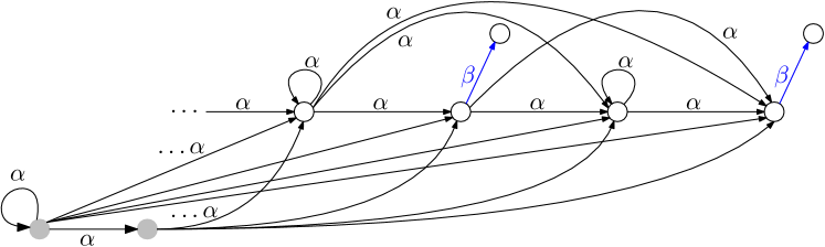
Figure 3: Kripke structure for Theorem 5. $L=\{\alpha,\beta,\alpha.\beta\}$; all black arrows have label $\alpha$; $\alpha.\beta$ transitions are not shown but span each concatenated $\alpha$ transition and $\beta$ transition.

The proof of the claim in Example 5 is nontrivial, and as far as we know, there are no results even suggesting that such Kripke structures exist. Importantly, Example 5 implies a similar example for GSTs because it contains a Kripke structure that also satisfies the schemata in Theorem 11. The following example makes this explicit.

Example 6.

Recall the definition of $G_{A}$ from Example 4, and consider the GST $G_{X}$ for $X=\{1/2+1/(n+2):n\in\mathbb{N}\}\subset(0,1)$. Then $G_{X}$ doesn’t belong to any VHHM class of GSTs because its surrogate Kripke structure is bisimilar to the Kripke structure in Example 5 (when it is suitably relabeled).

6 Conclusions and Future Work

In this paper we have proposed a generalization of Hennessy-Milner logic that is suitable for GSTs, and we have used this logic to exhibit some results regarding Hennessy-Milner classes with respect to weak bisimulation. Nevertheless, there is a great deal of work still to be done. One key avenue of future research lies in deciding whether the characterization in Theorem 11 really describes all maximal VHHM classes of GSTs (given a sufficiently large set of GSTs to begin with). Another important avenue of future work is to investigate what implications these VHHM classes have for common hybrid system models, such as the behavioral modeling framework of [19].

References

- [1]
- [2] Carlos E. Budde, Pedro R. D’Argenio, Pedro Sánchez Terraf & Nicolás Wolovick (2014): A Theory for the Semantics of Stochastic and Non-deterministic Continuous Systems. In: Stochastic Model Checking. Rigorous Dependability Analysis Using Model Checking Techniques for Stochastic Systems, Lecture Notes in Computer Science, Springer, Berlin, Heidelberg, pp. 67–86, 10.1007/978-3-662-45489-3_3.
- [3] Rance Cleaveland (1990): On automatically explaining bisimulation inequivalence. In: International Conference on Computer Aided Verification, Springer, pp. 364–372, 10.1007/BFb0023750.
- [4] Pedro R. D’Argenio & Pedro Sánchez Terraf (2012): Bisimulations for non-deterministic labelled Markov processes. Mathematical Structures in Computer Science 22(1), pp. 43–68, 10.1017/S0960129511000454.
- [5] J M Davoren & Paulo Tabuada (2007): On Simulations and Bisimulations of General Flow Systems. In: Hybrid Systems: Computation and Control, Springer Berlin Heidelberg, Berlin, Heidelberg, pp. 145–158, 10.1007/978-3-540-71493-4_14.
- [6] Josée Desharnais, Abbas Edalat & Prakash Panangaden (2002): Bisimulation for Labelled Markov Processes. Information and Computation 179(2), pp. 163–193, 10.1006/inco.2001.2962.
- [7] E. Doberkat (2005): Stochastic Relations: Congruences, Bisimulations and the Hennessy–Milner Theorem. SIAM Journal on Computing 35(3), pp. 590–626, 10.1137/S009753970444346X.
- [8] Ernst-Erich Doberkat (2007): The Hennessy–Milner equivalence for continuous time stochastic logic with mu-operator. Journal of Applied Logic 5(3), pp. 519–544, 10.1016/j.jal.2006.05.001.
- [9] Ernst-Erich Doberkat & Pedro Sánchez Terraf (2017): Stochastic non-determinism and effectivity functions. Journal of Logic and Computation 27(1), pp. 357–394, 10.1093/logcom/exv049.
- [10] James Ferlez, Rance Cleaveland & Steve Marcus (2014): Generalized Synchronization Trees. In: Foundations of Software Science and Computation Structures (FoSSaCS), Springer Berlin Heidelberg, Berlin, Heidelberg, pp. 304–319, 10.1007/978-3-642-54830-7_20.
- [11] Robert Goldblatt (1992): Logics of Time and Computation, Second edition. CSLI Lecture Notes, Stanford University, Center for the Study of Language and Information. Available at http://www.press.uchicago.edu/ucp/books/book/distributed/L/bo3615704.html.
- [12] Robert Goldblatt (1995): Saturation and the Hennessy-Milner Property. In Alban Ponse, Maarten de Rijke & Yde Venema, editors: Modal Logic and Process Algebra: A Bisimulation Perspective, Center for the Study of Language and Information Publication Lecture Notes, Cambridge University Press, pp. 107–129.
- [13] Valentin Goranko & Martin Otto (2007): Model theory of modal logic. In Johan Van Benthem and Frank Wolter Patrick Blackburn, editor: Studies in Logic and Practical Reasoning, Handbook of Modal Logic 3, Elsevier, pp. 249–329, 10.1016/S1570-2464(07)80008-5.
- [14] Matthew Hennessy & Robin Milner (1985): Algebraic laws for nondeterminism and concurrency. Journal of the ACM, 10.1145/2455.2460.
- [15] Marco Hollenberg (1995): Hennessy-Milner Classes and Process Algebra. In Alban Ponse, Maarten de Rijke & Yde Venema, editors: Modal Logic and Process Algebra: A Bisimulation Perspective, Center for the Study of Language and Information Publication Lecture Notes, Cambridge University Press, pp. 187–216.
- [16] Thomas Jech (2003): Set Theory, Third Millenium edition. Springer Monographs in Mathematics, Springer-Verlag Berlin Heidelberg, 10.1007/3-540-44761-X.
- [17] Robin Milner (1990): Operational and Algebraic Semantics of Concurrent Processes. In: Handbook of Theoretical Computer Science (Vol. B), MIT Press, Cambridge, MA, USA, pp. 1201–1242, 10.1016/B978-0-444-88074-1.50024-X.
- [18] Pedro Sánchez Terraf (2015): Bisimilarity is not Borel. Mathematical Structures in Computer Science, pp. 1–20, 10.1017/S0960129515000535.
- [19] Jan Willems (2007): The Behavioral Approach to Open and Interconnected Systems. IEEE Control Systems Magazine 27(6), pp. 46–99, 10.1109/MCS.2007.906923.