AN UNKNOTTING INDEX FOR VIRTUAL KNOTS

K. KAUR, S. KAMADA, A. KAWAUCHI and M. PRABHAKAR

Abstract

In this paper we introduce the notion of an unknotting index for virtual knots. We give some examples of computation by using writhe invariants, and discuss a relationship between the unknotting index and the virtual knot module. In particular, we show that for any non-negative integer $n$ there exists a virtual knot whose unknotting index is $(1,n)$.

1 Introduction

Virtual knot theory was introduced by L. H. Kauffman [11] as a generalization of classical knot theory. A diagram of a virtual knot may have virtual crossings which are encircled by a small circle and are not regarded as (real) crossings. A virtual knot is an equivalence class of diagrams where the equivalence is generated by moves in Figs. 1 and 2.

The purpose of this paper is to introduce an unknotting index $U(K)$ for a virtual knot, whose idea is an extension of the usual unknotting number for classical knots. The unknotting index of a virtual knot is a pair of non-negative integers which is considered as an ordinal number with respect to the dictionary order. The definition is given in Section 2. As the usual unknotting number for classical knots, it is not easy to determine the value of the unknotting index of a given virtual knot. We provide some examples of computation by using writhe invariants of virtual knots in Section 4. In Section 5 we discuss the unknotting index using the virtual knot module. An estimation of the unknotting index using the index $e(M)$ of the virtual knot module $M$ is given (Theorem 5.1). Then we show that for any non-negative integer $n$, there exists a virtual knot $K$ with $U(K)=(0,n)$ (Example 4.5 or Proposition 5.4) and there exists a virtual knot $K$ with $U(K)=(1,n)$ (Theorem 5.5).

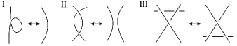
Figure 1: Classical Reidemeister moves: RI, RII and RIII

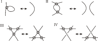
Figure 2: Virtual Reidemeister moves: VRI, VRII, VRIII and VRIV

2 An unknotting index for virtual knots

In this section, we define an unknotting index for virtual knots.

Let $D$ be a diagram of a virtual knot $K$. For a pair $(m,n)$ of non-negative integers, we say that $D$ is $(m,n)$-unknottable if the diagram $D$ is changed into a diagram of the trivial knot by changing $m$ crossings of $D$ into virtual crossings and by applying crossing change operations on $n$ crossings of $D$. Let ${\mathcal{U}}(D)$ denote the set of such pairs $(m,n)$. Note that $D$ is $(c(D),0)$-unknottable, where $c(D)$ is the number of crossings of $D$. Thus, ${\mathcal{U}}(D)$ is non-empty.

Definition 2.1.

• The unknotting index of a diagram $D$, denoted by $U(D)$, is the minimum among all pairs $(m,n)$ such that $D$ is $(m,n)$-unknottable. Namely, $U(D)$ is the minimum among the family ${\mathcal{U}}(D)$. (The minimality is taken with respect to the dictionary order.)

• The unknotting index of a virtual knot $K$, denoted by $U(K)$, is the minimum among all pairs $(m,n)$ such that $K$ has a diagram $D$ which is $(m,n)$-unknottable. Namely, $U(K)$ is the minimum among the family $\{U(D)\mid\mbox{$D$ presents $K$}\}$.

For example, when $D$ is the diagram on the left of Fig. 3, the figure shows that $(0,1)$ and $(2,0)$ belong to ${\mathcal{U}}(D)$. Since $(0,0)$ is not an element of ${\mathcal{U}}(D)$, we have $U(D)=(0,1)$. (Actually, ${\mathcal{U}}(D)=\{(0,1),(0,2),(1,1),(2,0),(2,1),(3,0)\}$. In order to determine $U(D)$ it is often unnecessary to find all elements of ${\mathcal{U}}(D)$.) Thus, for the left-handed trefoil $K$, $U(K)=(0,1)$. (Note that a virtual knot $K$ is trivial iff $U(K)=(0,0)$.)

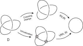
Figure 3:

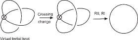
Figure 4:

For the (left-handed) virtual trefoil, which is presented by the diagram of the left of Fig. 4, $U(K)=(0,1)$.

A flat virtual knot diagram is a virtual knot diagram by forgetting the over/under-information of every real crossing. A flat virtual knot is an equivalence class of flat virtual knot diagrams by flat Reidemeister moves which are Reidemeister moves (Figs. 1 and 2) without the over/under-information.

Lemma 2.2.

Let $K$ be a virtual knot and $\overline{K}$ its flat projection. If $\overline{K}$ is non-trivial, then $U(K)\geq(1,0)$.

Proof: Assume that $U(K)=(0,n)$ for some $n$. There is a diagram $D$ of $K$ such that $D$ becomes a diagram of the trivial knot by $n$ crossing changes. The flat virtual knot diagram $\overline{D}$ obtained from $D$ is a diagram of the trivial knot, which implies $\overline{K}$ is trivial. $\square$

Example 2.3.

Let $D$ be the diagram depicted in Fig. 5 and $K$ the virtual knot presented by $D$, which is called Kishino’s knot. It is nontrivial as a virtual knot (cf. [1, 7, 9, 16, 17]) and the flat projection $\overline{K}$ is nontrivial as a flat virtual knot (cf. [7, 9]). Thus $U(K)\geq(1,0)$. It is easily seen that $D$ is $(1,0)$-unknottable. Therefore, $U(K)=(1,0)$.

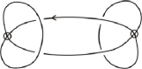
Figure 5: Kishino’s knot

3 Gauss diagrams and writhe invariants

We recall Gauss diagrams and writhe invariants of virtual knots. In what follows, we assume that virtual knots are oriented.

A Gauss diagram of a virtual knot diagram $D$ is an oriented circle where the pre-images of the over crossing and under crossing of each crossing are connected by a chord. To indicate the over/under-information, chords are directed from the over crossing to the under. Corresponding to each crossing $c$ in a virtual knot diagram, there are two points $\overline{c}$ and $\underline{c}$ which present the over crossing and the under crossing for $c$ in the oriented circle. The sign of each chord is the sign of the corresponding crossing. The sign of a crossing or a chord $c$ is also called the writhe of $c$ and denoted by $w(c)$ in this paper.

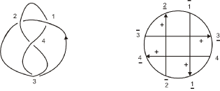
Figure 6: Gauss diagram for a diagram of the figure eight knot

In terms of a Gauss diagram, virtualizing a crossing of a diagram corresponds to elimination of a chord, and a crossing change corresponds to changing the direction and the sign of a chord. In what follows, for a Gauss diagram, we refer to changing the direction and the sign of a chord $c$ as a crossing change at $c$.

Writhe invariants were defined by some researchers independently. The writhe polynomial was defined by Cheng–Gau [2], which is equivalent to the affine index polynomial defined by Kauffman [13]. Satoh–Taniguchi [20] introduced the $k$-th writhe $J_{k}$ for each $k\in{\mathbb{Z}}\setminus\{0\}$, which is indeed a coefficient of the affine index polynomial. (Invariants related to these are found in Cheng [3], Dye [5] and Im–Kim–Lee [8].)

The writhe polynomial $W_{G}(t)$ stated below is the one in [2] multiplied by $t^{-1}$. This convention makes it easier to see the relationship between $W_{G}(t)$ and the affine index polynomial or the $k$-th writhe $J_{k}$.

Let $c$ be a chord of a Gauss diagram $G$. Let $r_{+}$ (respectively, $r_{-}$) be the number of positive (resp. negative) chords intersecting with $c$ transversely from right to left when we see them from the tail toward the head of $c$. Let $l_{+}$ (respectively, $l_{-}$) be the number of positive (resp. negative) chords intersecting with $c$ transversely from left to right. The index of $c$ is defined as

$${\rm Ind}(c)=r_{+}-r_{-}-l_{+}+l_{-}.$$

The writhe polynomial $W_{G}(t)$ of $G$ is defined by

$$W_{G}(t)=\sum_{c~{}:~{}{\rm Ind}(c)\neq 0}w(c)t^{{\rm Ind}(c)}.$$

For each integer $k$, the $k$-th writhe $J_{k}(G)$ is the number of positive chords with index $k$ minus that of negative ones with index $k$. Then

$$W_{G}(t)=\sum_{k\neq 0}J_{k}(G)t^{k}.$$

The $k$-th writhe $J_{k}(G)$ is an invariant of the virtual knot presented by $G$ when $k\neq 0$.

The writhe polynomial $W_{K}(t)$ and the $k$-th writhe $J_{k}(K)$ of a virtual knot $K$ is defined by those for a Gauss diagram presenting $K$.

The odd writhe $J(G)$ defined by Kauffman [12] is

$$\sum_{c\in Odd(G)}w(c),$$

where $w(c)$ denotes the writhe and $Odd(G)$ is the set of chords with odd indices.

4 Unknotting indices of some virtual knots

We give examples of computation of the unknotting indices for some virtual knots using writhe invariants.

Lemma 4.1 ([20]).

Let $G$ and $G^{\prime}$ be Gauss diagrams such that $G^{\prime}$ is obtained from $G$ by a crossing change. Then one of the following occurs.

• $W_{G}(t)-W_{G^{\prime}}(t)=\epsilon(t^{m}+t^{-m})$ for some integer $m\in{\mathbb{Z}}\setminus\{0\}$ and $\epsilon\in\{\pm 1\}$.

• $W_{G}(t)=W_{G^{\prime}}(t)$

Proof: Let $c$ be the chord of $G$ such that a crossing change at $c$ changes $G$ to $G^{\prime}$. Let $c^{\prime}$ be the chord of $G^{\prime}$ obtained from $c$ by the crossing change. Then ${\rm Ind}(c^{\prime})=-{\rm Ind}(c)$ and $w(c^{\prime})=-w(c)$. For any chord $d$ of $G$, except $c$, the index ${\rm Ind}(d)$ and the writhe $w(d)$ are preserved by the crossing change at $c$. When ${\rm Ind}(c)\neq 0$, let $m={\rm Ind}(c)$ and $\epsilon=w(c)$, and we obtain the first case. When ${\rm Ind}(c)=0$, we have the second case. $\square$

By this lemma, we have the following.

Proposition 4.2 (cf. Theorem 1.5 of [20]).

Let $K$ be a virtual knot.

• If $J_{k}(K)\neq J_{-k}(K)$ for some $k\in{\mathbb{Z}}\setminus\{0\}$, then $(1,0)\leq U(K)$.

• $(0,\sum_{k\neq 0}|J_{k}(K)|/2)\leq U(K)$.

Proof: (1) Suppose that $(1,0)>U(K)$. This implies that $K$ has a Gauss diagram $G$ which can be transformed by crossing changes into a Gauss diagram presenting the unknot. By Lemma 4.1, the writhe polynomial $W_{G}(t)$ must be reciprocal, i.e., $J_{k}(G)=J_{-k}(G)$ for all $k\in{\mathbb{Z}}\setminus\{0\}$. (This is (i) of Theorem 1.5 of [20].) This contradicts the hypothesis. Thus, $(1,0)\leq U(K)$.

(2) If $(1,0)\leq U(K)$, then the inequality holds. Thus, we consider the case of $(1,0)>U(K)=(0,n)$. Let $G$ be a Gauss diagram of $K$ which can be transformed by $n$ crossing changes into a Gauss diagram presenting the unknot. By Lemma 4.1, we see that $\sum_{k\neq 0}|J_{k}(K)|\leq 2n$. $\square$

Remark 4.3.

If $K$ has a Gauss diagram $G$ which can be transformed by crossing changes into a Gauss diagram presenting the unknot, then $J_{k}(G)=J_{-k}(G)$ for all $k\in{\mathbb{Z}}\setminus\{0\}$. In this case, $\sum_{k\neq 0}|J_{k}(K)|/2=\sum_{k>0}|J_{k}(K)|=\sum_{k<0}|J_{k}(K)|$. (This is (ii) of Theorem 1.5 of [20].) Thus, we may say that $(0,\sum_{k>0}|J_{k}(K)|)\leq U(K)$ instead of the inequality in the second assertion of Proposition 4.2.

Corollary 4.4.

Let $K$ be a virtual knot and $J(K)$ the odd writhe. Then

$$(0,|J(K)/2|)\leq U(K).$$

Proof: By definition, $|J(K)|\leq\sum_{k\neq 0}|J_{k}(K)|$. The inequality in the second assertion of Proposition 4.2 implies the desired inequality. $\square$

We consider unknotting indices for some virtual knots.

Example 4.5.

Let $K$ be the virtual knot presented by a diagram $D$ depicted in Fig. 7 or Fig. 7(a). Then $U(K)=(0,n)$.

Proof: Since all crossings in $D$ are odd and have the same writhe, the odd writhe of $K$ is $\pm 2n$. By Corollary 4.4, $(0,n)\leq U(K)$. By crossing changes at crossings labelled with even numbers, we obtain a diagram of the trivial knot. Therefore $(0,n)\geq U(K)$. $\square$

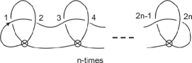
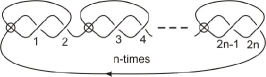
(a)

Figure 7:

Let $p$ be an odd integer. By a standard diagram of the $(2,p)$-torus knot, we mean a diagram obtained from a diagram of the $2$-braid $\sigma_{1}^{p}$ by taking closure.

Example 4.6.

If $K$ is a virtual knot presented by a diagram $D$ which is obtained from a standard diagram of the $(2,p)$-torus knot by virtualizing some crossings, then

$$U(K)\leq(0,c/2),$$

where $c$ is the number of crossings of $D$. Moreover, if $c$ is even then $U(K)=(0,c/2)$.

Proof: Let $G$ be the Gauss diagram corresponding to the diagram $D$ of $K$. An example is shown in Fig. 8. When $c\geq 2$, there exists a pair of chords as in Fig. 9, which can be removed by a crossing change at one of the chords and an RII move. If the resulting Gauss diagram still has such a pair of chords, then we remove the chords by a crossing change and an RII move. In this way, we can change $G$ into a Gauss diagram presenting the trivial knot by at most $c/2$ crossing changes. Hence, $U(K)\leq(0,c/2)$. If $c$ is even, then each chord of $G$ is an odd chord. The odd writhe of $K$ is $\pm c$. By Corollary 4.4, $(0,c/2)\leq U(K)$. Hence $U(K)=(0,c/2)$. $\square$

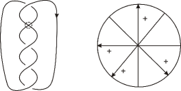
Figure 8: Closure of a virtual 2-braid with $U(K)=(0,2)$

Figure 9:

Next, we consider a virtual knot presented by a diagram obtained from a diagram of a twisted knot.

Let $D_{0}$ be the diagram illustrated in Fig. 10, which we call a standard diagram of a twisted knot. All crossings of $D_{0}$ except the crossings labeled $1$ and $2$ are positive. The signs of crossings labeled $1$ and $2$ are the same, which depends on the number of crossings.

Let $D$ be a diagram obtained from $D_{0}$ by virtualizing some crossings. Let $K$ be the virtual knot presented by $D$.

If the crossings labeled 1 and 2 in Fig. 10 are both virtualized in $D$, then the diagram $D$ presents the trivial knot. Hence $U(K)=(0,0)$.

If the crossings labeled 1 and 2 in Fig. 10 are intact, then $U(K)\leq(0,1)$. In particular, if $K$ is nontrivial, then $U(K)=(0,1)$.

Let $K$ be a virtual knot presented by a diagram $D$ which is obtained from a standard diagram $D_{0}$ of a twisted knot by virtualizing some crossings such that exactly one of the crossings labeled 1 and 2 ( in Fig. 10) is virtualized. The Gauss diagram $G$ corresponding to $D$ is as shown in Fig. 10, where the directions of horizontal chords are shown as an example. (The directions of horizontal chords depend on the parity of the number of crossings of $D_{0}$ and on the positions where we apply virtualization.) For convenience, let $c$ be the chord which intersects all other chords in $G$ as in Fig. 10. Let $l$ (or $r$) be the number of chords of $G$ intersecting with $c$ from left to right (or right to left) when we see the Gauss diagram as in Fig. 10, where we forget the direction of $c$. Recall that all horizontal chords have positive writhe.

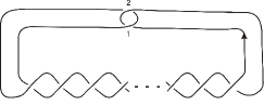
Figure 10:

Example 4.7.

Let $K$ be a virtual knot presented by a diagram $D$ which is obtained from a standard twisted knot diagram by virtualizing some crossings such that exactly one of the crossings labeled 1 and 2 ( in Fig. 10) is virtualized. Then

$$U(K)=\begin{cases}(0,|J(K)/2|),&\mbox{ if $|l-r|\leq 1$ }\\ (1,0),&\mbox{otherwise}\end{cases}$$

where $l$ and $r$ are the numbers described above.

Proof: Let $G$ be the Gauss diagram of $D$.

1. Suppose that $|l-r|\leq 1$. We observe that by crossing changes, i.e., changing the directions and the signs, of some chords in $G$, we can change $G$ into a Gauss diagram presenting the trivial knot. If there exists a pair of chords as in Fig. 11 in $G$, then by a crossing change and an RII move, we can remove the pair. If the resulting Gauss diagram still has such a pair of chords, then we remove the chords by a crossing change and an RII move. Repeat this procedure until we get a Gauss diagram $G_{1}$ whose horizontal chords are all directed in the same direction.

Figure 11:

• When $l=r$, the Gauss diagram $G_{1}$ has only one chord $c$, which presents a trivial knot. The number of crossing changes is $l$. On the other hand, all chords of $G$ except $c$ are odd chords having positive writhe. The odd writhe number $J(K)$ is $2l$. By Corollary 4.4, $U(K)=(0,l)=(0,|J(K)/2|)$.

• When $l=r+1$, the Gauss diagram $G_{1}$ has two chords, $c$ and a horizontal chord $c_{1}$, by $r$ times of crossing changes. Since all horizontal chords are positive, $J(K)=J(G)=l+r+w(c)$.

  • Suppose that $w(c)=-1$. In this case, the Gauss diagram $G_{1}$ presents the trivial knot. Thus we have $U(K)\leq(0,r)$. On the other hand, $J(K)=2r$. By Corollary 4.4, we have $U(K)=(0,|J(K)/2|)$.

  • Suppose that $w(c)=1$. Apply a crossing change to $G_{1}$ at $c_{1}$ and obtain a Gauss diagram $G_{2}$ with two chords $c$ and $c_{2}$ where $c_{2}$ is the horizontal chord obtained from $c_{1}$ with $w(c_{2})=-1$. Since $G_{2}$ presents the trivial knot, we have $U(K)\leq(0,l)$. On the other hand, $J(K)=2l$. By Corollary 4.4, we have $U(K)=(0,|J(K)/2|)$.

• When $r=l+1$, by a similar argument as above, we see that $U(K)=(0,|J(K)/2|)$.

2. Suppose that $|l-r|>1$. Let $c_{1},c_{2}\dots,c_{n}$ be the horizontal chords of $G$. For $i=1,\dots,n$, the index ${\rm Ind}(c_{i})$ is $1$ or $-1$. Note that ${\rm Ind}(c)=r-l$ or $l-r$ according to the direction of $c$ is upward or downward. Let $k={\rm Ind}(c)$. Then $J_{k}(G)=w(c)$ and $J_{-k}(G)=0$. By Proposition 4.2, $(1,0)\leq U(K)$.

Removing the chord $c$ from $G$, we obtain a Gauss diagram presenting the trivial knot. Hence, $U(K)=(1,0)$. $\square$

We used writhe invariants for lower bounds for the unknotting number. A research using the arrow polynomial (Dye–Kauffman [6]) or equivalently Miyazawa polynomial (Miyazawa [17, 18]) by the first and the fourth authors will be discussed elsewhere.

5 From the virtual knot module

In this section we discuss the unknotting index from a point view of the virtual knot module.

The group of a virtual knot is defined by a Wirtinger presentation obtained from a diagram as usual as in classical knot theory [11]. A geometric interpretation of the virtual knot group is given in [10] and a characterization of the group is in [19, 21].

For the group $G$ of a virtual knot $K$, let $G^{\prime}$ and $G^{\prime\prime}$ be the commutator subgroup and the second commutator subgroup of $G$. Then the quotient group $M=G^{\prime}/G^{\prime\prime}$ forms a finitely generated $\Lambda$-module, called the virtual knot module, where $\Lambda={\mathbb{Z}}[t,t^{-1}]$ denotes the Laurent polynomial ring. A characterization of a virtual knot module is given by [15, Theorem 4.3]. Let $e(M)$ be the minimal number of $\Lambda$-generators of $M$. Then the following.

Theorem 5.1.

If $U(K)=(m,n)$, then $e(M)\leq m+n$.

Theorem 5.1 is obtained from the following lemma.

Lemma 5.2.

Let $K$ and $K_{1}$ be virtual knots, and let $M$ and $M_{1}$ be their virtual knot modules. Suppose that a diagram of $K_{1}$ is obtained from a diagram of $K$ by $(1)$ virtualizing a crossing or by $(2)$ a crossing change. Then $|e(M)-e(M_{1})|\leq 1$.

Proof: Suppose that a diagram $D_{1}$ of $K_{1}$ is obtained from a diagram $D$ of $K$ by virtualizing a crossing or a crossing change at a crossing $c$.

Let $P=(x_{1},x_{2},\dots,x_{u}|r_{1},r_{2},\dots,r_{v})$ be a Wirtinger presentation of the group $G$ of $K$ obtained from $D$ with edge generators $x_{1},x_{2},\dots,x_{u}$ such that the last word $r_{v}$ is $x_{u}^{-1}x_{i}^{-1}x_{u-1}x_{i}$ for an $i<u-1$ which is a relation around the crossing $c$.

Let $P_{0}=(x_{1},x_{2},\dots,x_{u-1}|\,\tilde{r}_{1},\tilde{r}_{2},\dots,\tilde{r}_{v})$ be the group presentation of a group $G_{0}$ obtained from $P$ by writing the letter $x_{u}$ to $x_{u-1}$ and rewriting the words $r_{1},r_{2},\dots,r_{v}$ as the words $\tilde{r}_{1},\tilde{r}_{2},\dots,\tilde{r}_{v}$ in the letters $x_{1},x_{2},\dots,x_{u-1}$. Then the word $\tilde{r}_{v}$ is given by $x_{u-1}^{-1}x_{i}^{-1}x_{u-1}x_{i}$.

(1) We consider the case of virtualizing the crossing $c$. The group $G_{1}$ of $K_{1}$ has the Wirtinger presentation $P_{1}=(x_{1},x_{2},\dots,x_{u-1}|\,\tilde{r}_{1},\tilde{r}_{2},\dots,\tilde{r}_{v-1})$.

We have the following $\Lambda$-semi-exact sequence

$$\Lambda[r_{1}^{*},r_{2}^{*},\dots,r_{v}^{*}]\stackrel{{\scriptstyle d_{2}}}{{\to}}\Lambda[x_{1}^{*},x_{2}^{*},\dots,x_{u}^{*}]\stackrel{{\scriptstyle d_{1}}}{{\to}}\Lambda\stackrel{{\scriptstyle\varepsilon}}{{\to}}{\mathbb{Z}}\to 0$$

of the presentation $P$ by using the fundamental formula of the Fox differential calculus in [4], where $\Lambda[r_{1}^{*},r_{2}^{*},\dots,r_{v}^{*}]$ and $\Lambda[x_{1}^{*},x_{2}^{*},\dots,x_{u}^{*}]$ are free $\Lambda$-modules with bases $r_{i}^{*}$ ($i=1,2,\dots,v$) and $x_{j}^{*}$ ($j=1,2,\dots,u$), respectively, and the $\Lambda$-homomorphisms $\varepsilon$, $d_{1}$ and $d_{2}$ are given as follows:

$$\varepsilon(t)=1,\,\,d_{1}(x_{j}^{*})=t-1\,(j=1,2,\dots,u),\,\,d_{2}(r_{i}^{*})=\sum_{j=1}^{u}\frac{\partial r_{i}}{\partial x_{j}}x^{*}_{j}\,(i=1,2,\dots,v)$$

for the Fox differential calculus $\frac{\partial r_{i}}{\partial x_{j}}$ regarded as an element of $\Lambda$ by letting $x_{j}$ to $t$. (Here a $\Lambda$-semi-exact sequence means that, in the above sequence, it is a chain complex of $\Lambda$-modules with $\mbox{Im}(d_{1})=\mbox{Ker}(\varepsilon)$ and $\mbox{Im}(\varepsilon)={\mathbb{Z}}$.) The $\Lambda$-module $M$ of $G$ is identified with the quotient $\Lambda$-module $\mbox{Ker}(d_{1})/\mbox{Im}(d_{2})$.

Similarly, we have the $\Lambda$-semi-exact sequences

$$\Lambda[\tilde{r}_{1}^{*},\tilde{r}_{2}^{*},\dots,\tilde{r}_{v-1}^{*},\tilde{r}_{v}^{*}] \stackrel{{\scriptstyle\tilde{d}_{2}}}{{\to}} \Lambda[x_{1}^{*},x_{2}^{*},\dots,x_{u-1}^{*}]\stackrel{{\scriptstyle\tilde{d}_{1}}}{{\to}}\Lambda\stackrel{{\scriptstyle\varepsilon}}{{\to}}{\mathbb{Z}}\to 0,\quad\mbox{and}$$

$$\Lambda[\tilde{r}_{1}^{*},\tilde{r}_{2}^{*},\dots,\tilde{r}_{v-1}^{*}] \stackrel{{\scriptstyle\tilde{d}^{\prime}_{2}}}{{\to}} \Lambda[x_{1}^{*},x_{2}^{*},\dots,x_{u-1}^{*}]\stackrel{{\scriptstyle\tilde{d}_{1}}}{{\to}}\Lambda\stackrel{{\scriptstyle\varepsilon}}{{\to}}{\mathbb{Z}}\to 0$$

of the presentations $P_{0}$ and $P_{1}$, respectively, where the $\Lambda$-homomorphism $\tilde{d}^{\prime}_{2}$ is the restriction of the $\Lambda$-homomorphism $\tilde{d}_{2}$. The $\Lambda$-modules $M_{0}$ and $M_{1}$ of $G_{0}$ and $G_{1}$ are identified with the quotient $\Lambda$-modules $\mbox{Ker}(\tilde{d}_{1})/\mbox{Im}(\tilde{d}_{2})$ and $\mbox{Ker}(\tilde{d}_{1})/\mbox{Im}(\tilde{d}^{\prime}_{2})$, respectively.

The epimorphism $G\to G_{0}$ induces a commutative ladder diagram from the $\Lambda$-semi-exact sequence of $P$ to the $\Lambda$-semi-exact sequence of $P_{0}$ by sending $r_{i}^{*}$ to $\tilde{r}_{i}^{*}$ for all $i$, $x_{j}^{*}$ to $x_{j}^{*}$ for all $j\leq u-1$ and $x_{u}^{*}$ to $x_{u-1}^{*}$. Then the short $\Lambda$-exact sequence

$$0\to\Lambda[x_{u}^{*}-x_{u-1}^{*}]\to\Lambda[x_{1}^{*},x_{2}^{*},\dots,x_{u}^{*}]\to\Lambda[x_{1}^{*},x_{2}^{*},\dots,x_{u-1}^{*}]\to 0$$

induces a $\Lambda$-exact sequence $\Lambda\to M\to M_{0}\to 0$, giving

$$e(M_{0})\leq e(M)\leq e(M_{0})+1.$$

On the other hand, the epimorphism $G_{1}\to G_{0}$ induces a commutative ladder diagram from the $\Lambda$-semi-exact sequence of $P_{1}$ to the $\Lambda$-semi-exact sequence of $P_{0}$ by sending $\tilde{r}_{i}^{*}$ to $\tilde{r}_{i}^{*}$ for all $i\leq v-1$ and $x_{j}^{*}$ to $x_{j}^{*}$ for all $j\leq u-1$. Then from the short exact sequence

$$0\to\mbox{Im}(\tilde{d}_{2})/\mbox{Im}(\tilde{d}^{\prime}_{2})\to\mbox{Ker}(\tilde{d}_{1})/\mbox{Im}(\tilde{d}^{\prime}_{2})\to\mbox{Ker}(\tilde{d}_{1})/\mbox{Im}(\tilde{d}_{2})\to 0$$

and an epimorphism $\Lambda[\tilde{r}_{v}^{*}]\to\mbox{Im}(\tilde{d}_{2})/\mbox{Im}(\tilde{d}^{\prime}_{2})$, a $\Lambda$-exact sequence $\Lambda\to M_{1}\to M_{0}\to 0$ is obtained, giving

$$e(M_{0})\leq e(M_{1})\leq e(M_{0})+1.$$

Thus, the inequality $|e(M)-e(M_{1})|\leq 1$ is obtained.

(2) We consider the case of a crossing change at $c$. As seen in (1), we have

$$e(M_{0})\leq e(M)\leq e(M_{0})+1.$$

Note that the module $M_{0}$ is the $\Lambda$-module of the group $G_{0}$, which is obtained from the virtual knot diagram $D$ with $c$ virtualized by adding a relation that two edge generators around the virtualized $c$ commute. When we apply the same argument with $D_{1}$ instead of $D$, we have the same module $M_{0}$ and

$$e(M_{0})\leq e(M_{1})\leq e(M_{0})+1.$$

Thus the inequality $|e(M)-e(M_{1})|\leq 1$ is obtained. $\square$

Remark 5.3.

We have an alternative and somewhat geometric proof of the case of a crossing change in Lemma 5.2 as follow: Suppose that a diagram $D_{1}$ of $K_{1}$ is obtained from a diagram $D$ of $K$ by a crossing change. The virtual knot group $G$ is considered as the fundamental group $\pi_{1}(E,*)$ of the complement $E=X^{*}\setminus K$ of a knot $K$ in a singular 3-manifold $X^{*}$ which is obtained from the product $X=F\times[0,1]$ with $F$ a closed oriented surface by shrinking $X_{0}=F\times 0$ to a point $*$, where the knot $K$ is in the interior of $X$ (see [10]). The virtual knot group $G_{1}$ is the fundamental group $\pi_{1}(E_{1},*)$ of a singular 3-manifold $E_{1}$ obtained from $E$ by surgery along a pair of 2-handles. Since the virtual knot modules $M$ and $M_{1}$ are $\Lambda$-isomorphic to the first homology $\Lambda$-modules $H_{1}(\tilde{E};{\mathbb{Z}})$ and $H_{1}(\tilde{E}_{1};{\mathbb{Z}})$ for the infinite cyclic covering spaces $\tilde{E}$ and $\tilde{E}_{1}$ of $E$ and $E_{1}$, respectively, the argument of [14, Theorem 2.3] implies that $|e(M)-e(M_{1})|\leq 1$.

Proposition 5.4.

For any non-negative integer $n$, there exists a virtual knot $K$ with $U(K)=(0,n)$.

Proof: If $n=1$, then let $K$ be the unknot. Assume $n\geq 1$. Let $K$ be the $n$-fold connected sum of a trefoil knot without virtual crossings. Then $e(M)=n$. Since we know $U(K)\leq(0,n)$, Theorem 5.1 implies $U(K)=(0,n)$. $\square$

Theorem 5.5.

For any non-negative integer $n$, there exists a virtual knot $K$ with $U(K)=(1,n)$.

Proof: Let $D_{0}$ be a virtual knot diagram obtained from the diagram in Fig. 5 by applying crossing change at the two crossings on the left side, and let $K_{0}$ be the virtual knot presented by $D_{0}$. The group of $K_{0}$ is isomorphic to the group of a trefoil knot. Let $K$ be the connected sum of $K_{0}$ and the $n$-fold connected sum of a trefoil knot such that a diagram $D$ of $K$ is a connected sum of $D_{0}$ and a diagram of the $n$-fold connected sum of a trefoil knot without virtual crossings. Then the group of $K$ is isomorphic to the group of the $(n+1)$-fold connected sum of a trefoil knot and $e(M)=n+1$. Since $U(K)\leq U(D)\leq(1,n)$, by Theorem 5.1, we have $U(K)=(1,n)$ or $(0,n+1)$. On the other hand, when we consider the flat projection $\overline{K}$ of $K$, $\overline{K}$ is the same with the flat projection $\overline{K_{0}}$ of $K_{0}$, which is non-trivial. By Lemma 2.2, we have $U(K)=(1,n)$. $\square$

We conclude with a problem for future work.

Find a virtual knot $K$ with $U(K)=(m,n)$ for a given $(m,n)$. A connected sum of $m$ copies of Kishino’s knot (or $K_{0}$ in the proof of Theorem 5.5) and $n$ copies of a trefoil knot seems a candidate.

References

- [1] A. Bartholomew and R. Fenn: Quaternionic invariants of virtual knots and links, J. Knot Theory Ramifications 17 (2008), 231–251.
- [2] Z. Cheng and H. Gao: A polynomial invariant of virtual links, J. Knot Theory Ramifications 22 (2013), 1341002.
- [3] Z. Cheng: A polynomial invariant of virtual knots, Proc. Amer. Math. Soc. 142 (2014), 713–725.
- [4] R. H. Crowell and R. H. Fox: Introduction to Knot Theory, Ginn and Co., Boston, Mass., 1963.
- [5] H. Dye: Vassiliev invariants from parity mappings, J. Knot Theory Ramifications 22 (2013), 1340008.
- [6] H. A. Dye and L. H. Kauffman: Virtual crossing number and the arrow polynomial, J. Knot Theory Ramifications 18 (2009), 1335–1357.
- [7] R. Fenn and V. Turaev: Weyl algebras and knots, J. Geom. Phys. 57 (2007), 1313–1324.
- [8] Y. H. Im, S. Kim, and D. S. Lee: The parity writhe polynomials for virtual knots and flat virtual knots, J. Knot Theory Ramifications 22 (2013), 1250133.
- [9] T. Kadokami: Detecting non-triviality of virtual links, J. Knot Theory Ramifications 12 (2003), 781–803.
- [10] N. Kamada and S. Kamada: Abstract link diagrams and virtual knots, J. Knot Theory Ramifications 9 (2000), 93–106.
- [11] L. H. Kauffman: Virtual knot theory, European J. Combin. 20 (1999), 663–690.
- [12] L. H. Kauffman: A self-linking invariant of virtual knots, Fund. Math. 184 (2004), 135–158.
- [13] L. H. Kauffman: An affine index polynomial invariant of virtual knots, J. Knot Theory Ramifications 22 (2013), 1340007.
- [14] A. Kawauchi: Distance between links by zero-linking twists, Kobe J. Math. 13 (1996), 183–190.
- [15] A. Kawauchi: The first Alexander Z(Z)-modules of surface-links and of virtual links, Geometry and Topology Monographs 14 (2008), 353–371.
- [16] T. Kishino and S. Satoh: A note on classical knot polynomials, J. Knot Theory Ramifications 13 (2004), 845–856.
- [17] Y. Miyazawa: A multi-variable polynomial invariant for virtual knots and links, J. Knot Theory Ramifications 17 (2008), 1311–1326.
- [18] Y. Miyazawa: A virtual link polynomial and the crossing number, J. Knot Theory Ramifications 18 (2009), 605–623.
- [19] S. Satoh: Virtual knot presentation of ribbon torus-knots, J. Knot Theory Ramifications 9 (2000), 531–542.
- [20] S. Satoh and K. Taniguchi: The writhes of a virtual knot, Fund. Math. 225 (2014), 327–342.
- [21] D. S. Silver and S. G. Williams: Virtual knot groups, Knots in Hellas ’98 (Delphi), 440–451, Ser. Knots Everything, 24, World Sci. Publ., River Edge, NJ, 2000.
Kirandeep Kaur
Department of Mathematics
Indian Institute of Technology Ropar,
Punjab, India 140001
e-mail: kirandeep.kaur@iitrpr.ac.in
Seiichi Kamada
Department of Mathematics
Osaka City University,
Osaka 558-8585, Japan
e-mail: skamada@sci.osaka-cu.ac.jp
Akio Kawauchi
OCAMI, Osaka City University,
Osaka 558-8585, Japan
e-mail: kawauchi@sci.osaka-cu.ac.jp
Madeti Prabhakar
Department of Mathematics
Indian Institute of Technology Ropar,
Punjab, India 140001
e-mail: prabhakar@iitrpr.ac.in