The Averaged Kaczmarz Iteration for Solving Inverse Problems

Abstract

We introduce a new iterative regularization method for solving inverse problems that can be written as systems of linear or non-linear equations in Hilbert spaces. The proposed averaged Kaczmarz (AVEK) method can be seen as a hybrid method between the Landweber and the Kaczmarz method. As the Kaczmarz method, the proposed method only requires evaluation of one direct and one adjoint sub-problem per iterative update. On the other, similar to the Landweber iteration, it uses an average over previous auxiliary iterates which increases stability. We present a convergence analysis of the AVEK iteration. Further, detailed numerical studies are presented for a tomographic image reconstruction problem, namely the limited data problem in photoacoustic tomography. Thereby, the AVEK is compared with other iterative regularization methods including standard Landweber and Kaczmarz iterations, as well as recently proposed accelerated versions based on error minimizing relaxation strategies.

Keywords: Inverse problems, system of ill-posed equations, regularization method, Kaczmarz iteration, ill-posed equation, convergence analysis, tomography, circular Radon transform.

AMS Subject Classification: 65J20; 65J22; 45F05.

1 Introduction

In this paper, we study the stable solution of linear or non-linear systems of operator equations of the form

$$\mathbf{F}_{i}(\boldsymbol{x})=\boldsymbol{y}_{i}\quad\text{ for }i=1,\dots,n\,.$$ (1.1)

Here $\mathbf{F}_{i}\colon\operatorname*{\mathcal{D}}(\mathbf{F}_{i})\subseteq\mathbb{X}\to\mathbb{Y}_{i}$ are possibly nonlinear operators between Hilbert spaces $\mathbb{X}$ and $\mathbb{Y}_{i}$ with domains of definition $\operatorname*{\mathcal{D}}(\mathbf{F}_{i})$. We are in particular interested in the case that we only have approximate data $\boldsymbol{y}_{i}^{\delta}\in\mathbb{Y}_{i}$ available, which satisfy an estimate of the form $\|\boldsymbol{y}_{i}^{\delta}-\boldsymbol{y}_{i}\|\leq\delta_{i}$ for some noise levels $\delta_{i}>0$. Moreover, we focus on the ill-posed (or ill-conditioned) case, where standard solution methods for (1.1) are sensitive to perturbations. Many inverse problems in biomedical imaging, geophysics or engineering sciences can be written in such a form (see, for example, [16, 34, 43].) For its solution one has to use regularization methods, which are based on approximating (1.1) by neighboring but more stable problems.

There are at least two basic classes of solution approaches for inverse problems of the form (1.1), namely (generalized) Tikhonov regularization on the one and iterative regularization on the other hand. (Notice that there are methods sharing structures of both classes, for example iterated Tikhonov regularization [26] or Lardy’s method [30].) These approaches are based on rewriting (1.1) as a single equation $\mathbf{F}(\boldsymbol{x})=\boldsymbol{y}$ with forward operator $\mathbf{F}=(\mathbf{F}_{i})_{i=1}^{n}$ and exact data $\boldsymbol{y}=(\boldsymbol{y}_{i})_{i=1}^{n}$. In Tikhonov regularization, one defines approximate solutions as minimizers of the Tikhonov functional $\frac{1}{n}\sum_{i=1}^{n}\|\mathbf{F}_{i}(\boldsymbol{x})-\boldsymbol{y}^{\delta}_{i}\|^{2}+\lambda\|\boldsymbol{x}-\boldsymbol{x}_{0}\|^{2}$, which is the weighted combination of the residual term $\sum_{i=1}^{n}\|\mathbf{F}_{i}(\boldsymbol{x})-\boldsymbol{y}^{\delta}_{i}\|^{2}$ that enforces all equations to be approximately satisfied, and the regularization term $\|\boldsymbol{x}-\boldsymbol{x}_{0}\|^{2}$ that stabilizes the inversion process; $\lambda>0$ is usually referred to as the regularization parameter. In iterative regularization methods, stabilization is achieved via early stopping of iterative schemes. For this class of methods, one develops special iterative optimization techniques designed for minimizing the un-regularized residual term $\sum_{i=1}^{n}\|\mathbf{F}_{i}(\boldsymbol{x})-\boldsymbol{y}^{\delta}_{i}\|^{2}$. The iteration index in this case plays the role of the regularization parameter which has to be carefully chosen depending on available information about the noise and the unknowns to be recovered.

In this paper we introduce a new member of the class of iterative regularization methods, named averaged Kaczmarz (AVEK) iteration. The method combines advantages of two main iterative regularization techniques, namely the Landweber and the Kaczmarz iteration.

1.1 Iterative regularization methods

The most basic iterative method for solving inverse problems is the Landweber iteration [16, 21, 24, 29], which reads

$$\forall k\in\mathbb{N}\colon\quad\boldsymbol{x}^{\delta}_{k+1}\coloneqq\boldsymbol{x}^{\delta}_{k}-\frac{s_{k}}{n}\sum_{i=1}^{n}\mathbf{F}_{i}^{\prime}(\boldsymbol{x}^{\delta}_{k})^{*}\left(\mathbf{F}_{i}(\boldsymbol{x}_{k}^{\delta})-\boldsymbol{y}^{\delta}_{i}\right)\,.$$ (1.2)

Here $\mathbf{F}_{i}^{\prime}(\boldsymbol{x})^{*}$ is the Hilbert space adjoint of the derivative of $\mathbf{F}_{i}$, $s_{k}$ is the step size and $\boldsymbol{x}_{1}^{\delta}$ the initial guess. The Landweber iteration renders a regularization method when stopped according to Morozov’s discrepancy principle, which stops the iteration at the smallest index $k_{\star}$ such that $\sum_{i=1}^{n}\|\mathbf{F}_{i}(\boldsymbol{x}^{\delta}_{k_{\star}})-\boldsymbol{y}^{\delta}_{i}\|^{2}\leq n(\tau\delta)^{2}$ for some constant $\tau>1$. A convergence analysis of the non-linear Landweber iteration has first been derived in [21]. Among others, similar results have subsequently been established for the steepest-descent method [35], the preconditioned Landweber iteration [14], or Newton-type methods [6, 42].

Each iterative update in (1.2) can be numerically quite expensive, since it requires solving forward and adjoint problems for all of the $n$ equations in (1.1). In situations where $n$ is large and evaluating the forward and adjoint problems is costly, methods like the Landweber-Kaczmarz iteration (see [15, 19, 20, 25, 27])

$$\forall k\in\mathbb{N}\colon\quad\boldsymbol{x}^{\delta}_{k+1}\coloneqq\boldsymbol{x}^{\delta}_{k}-s_{k}\alpha_{k}\mathbf{F}_{[k]}^{\prime}(\boldsymbol{x}^{\delta}_{k})^{*}\left(\mathbf{F}_{[k]}(\boldsymbol{x}_{k}^{\delta})-\boldsymbol{y}^{\delta}_{[k]}\right)\,,$$ (1.3)

where $[k]\coloneqq(k-1\mod n)+1$, are often much faster. The acceleration comes from the fact that the update in (1.3) only requires the solution of one forward and one adjoint problem instead of solving several of them, but nevertheless often yields a comparable decrease per iteration of the reconstruction error. The additional parameters $\alpha_{k}\in\left\{0,1\right\}$ effect that in the noisy data case some of the iterative updates are skipped which renders (1.3) a regularization method. Such a skipping strategy has been introduced in [20] for the Landweber-Kaczmarz iteration and later, among others, combined with steepest descent and Levenberg-Marquardt type iterations [3, 12].

Kaczmarz type methods often perform well in practice. However, unless allowing asymptotically vanishing step sizes, even for well-posed problems, they do not converge to a single point. This can easily be seen in the case of two linear equations in $\mathbb{R}$ without a common solution where the Kaczmarz method with constant step size has different accumulation points [32, Section 2] (compare also [10, 45]). Opposed to that, the AVEK method that we introduce in this paper can be shown to converge in such a situation. Still, one step in AVEK has computational costs similar to the Kaczmarz method (if evaluating the forward operators and their adjoints are the computationally most expensive parts). Note that (1.2) and (1.3) might be called simultaneous and sequential, respectively [15, 23, 38, 39]. Further, instead of using the average in (1.2) one might also consider convex combinations of $\mathbf{F}_{i}^{\prime}(\boldsymbol{x}^{\delta}_{k})^{*}\left(\mathbf{F}_{i}(\boldsymbol{x}_{k}^{\delta})-\boldsymbol{y}^{\delta}_{i}\right)$ to define the iterative updates in simultaneous schemes (as is Cimmino’s method [11]).

1.2 The averaged Kaczmarz (AVEK) iteration

The general AVEK iteration is defined by

$$\boldsymbol{x}_{k+1}^{\delta} \coloneqq\sum_{\ell=k-n+1}^{k}\omega_{k-\ell+1}\boldsymbol{\xi}_{\ell}^{\delta}\qquad{\text{for }k\geq n}$$ (1.4)

$$\boldsymbol{\xi}_{\ell}^{\delta} \coloneqq\boldsymbol{x}_{\ell}^{\delta}-s_{\ell}\alpha_{\ell}\mathbf{F}_{[\ell]}^{\prime}(\boldsymbol{x}^{\delta}_{\ell})^{*}\left(\mathbf{F}_{[\ell]}(\boldsymbol{x}^{\delta}_{\ell})-\boldsymbol{y}^{\delta}_{[\ell]}\right)$$ (1.5)

$$\alpha_{\ell} \coloneqq\begin{cases}1&\text{if }\|\mathbf{F}_{[\ell]}(\boldsymbol{x}^{\delta}_{\ell})-\boldsymbol{y}^{\delta}_{[\ell]}\|\geq\tau_{[\ell]}\delta_{[\ell]}\\ 0&\text{otherwise}\end{cases}\,,$$ (1.6)

where $\boldsymbol{x}^{\delta}_{1},\ldots,\boldsymbol{x}^{\delta}_{n}$ are user-specified initial values, and $\omega_{i}\geq 0$ are fixed weights satisfying $\sum_{i=1}^{n}\omega_{i}=1$. Instead of discarding the previous computations, the AVEK iteration remembers the last Kaczmarz type auxiliary iterates $\boldsymbol{\xi}_{\ell}^{\delta}$ and the update $\boldsymbol{x}_{k+1}^{\delta}$ is defined as the weighted average over them. The parameters $\alpha_{\ell}$ effect that no update for $\boldsymbol{\xi}_{\ell}^{\delta}$ is performed if $\|\mathbf{F}_{[\ell]}(\boldsymbol{x}^{\delta}_{\ell})-\boldsymbol{y}^{\delta}_{[\ell]}\|$ is sufficiently small; $\tau_{i}\geq 0$ are control parameters. As the Kaczmarz iteration, the AVEK iteration only requires evaluating a single gradient $\mathbf{F}_{i}^{\prime}(\boldsymbol{x})^{*}(\mathbf{F}_{i}(\boldsymbol{x})-\boldsymbol{y}^{\delta}_{i})$ per iterative update which usually is the numerically most expensive part for evaluating (1.4)-(1.6). As the Landweber iteration (1.2), if every $\omega_{i}$ is positive, each update in AVEK uses information of all equations which enhances stability. Notice that the Landweber-Kaczmarz iteration in (1.3) is a special case of the general AVEK iteration with $\omega_{1}=1$ and $\omega_{i}=0$ for $i\geq 2$.

Throughout this paper, we focus on the AVEK with equal weights $\omega_{1}=\cdots=\omega_{n}=1/n$. In what follows, by AVEK we always refer to this special case unless explicitly stated. Note, that the AVEK update (1.4) in this case can alternatively be written as $\boldsymbol{x}^{\delta}_{k+1}=\boldsymbol{x}^{\delta}_{k}+(\boldsymbol{\xi}^{\delta}_{k}-\boldsymbol{\xi}^{\delta}_{k-n})/n$. The modified update formula only requires two additions in the space $\mathbb{X}$ and therefore can numerically be more efficient than evaluating (1.4). We further note that in the original form (1.4)-(1.6), AVEK requires storing $n$ auxiliary updates $\boldsymbol{\xi}_{\ell}^{\delta}\in\mathbb{X}$. When storage is a limited aspect and $n$ is large, this might be problematic. However, the required storage can be reduced by saving the residuals $\mathbf{F}_{[\ell]}(\boldsymbol{x}^{\delta}_{\ell})-\boldsymbol{y}^{\delta}_{[\ell]}\in\mathbb{Y}_{i}$ instead of the auxiliary updates. In the numerical implementation $\prod_{i=1}^{n}\mathbb{Y}_{i}$ (after discretization) will typically have a similar dimension as $\mathbb{X}$ (after discretization). As a consequence, storing all $n$ residuals only requires a storage similar to saving a single iterate.

In this paper we establish a convergence analysis of (1.4)-(1.6) for exact and noisy data (see Section 2). These results are most closely related to the convergence analysis of other iterative regularization methods such as the Landweber and steepest descent methods [21, 35] and extensions to Kaczmarz type iterations [12, 20, 31]. However, the AVEK iteration is new and we are not aware of a convergence analysis for any similar iterative regularization method. We point out, that the AVEK shares some similarities with the incremental gradient method of [7] and the averaged stochastic gradient method of [44] (both studied in finite dimensions). However, the iterations of [7, 44] are notably different from the AVEK method as they use an average of gradients instead of an average of auxiliary iterates (cf. Section 4). Given the large amount of publications on averaged incremental gradient and stochastic gradient methods over the last couple of years it seems surprising that these methods have not been extended in the spirit of AVEK so far. The present work might initiate future research in such directions.

1.3 Outline

The rest of this paper is organized as follows. In Section 2 we present the convergence analysis of the AVEK method under typical assumptions for iterative regularization methods. As main results we show weak convergence of AVEK in the case of exact data (see Theorem 2.7) and (weak and strong) convergence as the noise level tends to zero (see Theorem 2.10). The proof of an important auxiliary result (Lemma 2.5) required for the convergence analysis is presented in Appendix A. In Section 3, we apply AVEK method to the limited view problem for the circular Radon transform and present a numerical comparison with the Landweber and the Kaczmarz method. The paper concludes with a summary presented in Section 4 and a discussion of open issues and possible extensions of AVEK.

2 Convergence analysis

In this section we establish the convergence analysis of the AVEK method. For that purpose we first fix the main assumptions in Subsection 2.1 and derive the basic quasi-monotonicity property of AVEK in Subsection 2.2. The actual convergence analysis is presented in Subsections 2.3 and 2.4.

2.1 Preliminaries

Throughout this paper $\mathbf{F}_{i}\colon\operatorname*{\mathcal{D}}(\mathbf{F}_{i})\subseteq\mathbb{X}\to\mathbb{Y}_{i}$ are continuously Fréchet differentiable maps for $i\in\{1,\dots,n\}$. We consider the system (1.1), which can be written as a single equation $\mathbf{F}(\boldsymbol{x})=\boldsymbol{y}$ with forward operator $\mathbf{F}=(\mathbf{F}_{i})_{i=1}^{n}$ and exact data $\boldsymbol{y}=(\boldsymbol{y}_{i})_{i=1}^{n}$ in $\mathbb{Y}\coloneqq\prod_{i=1}^{n}\mathbb{Y}_{i}$. Here $\boldsymbol{y}\in\mathbb{Y}$ are the exact data and $\boldsymbol{y}^{\delta}=(\boldsymbol{y}_{i}^{\delta})_{i=1}^{n}\in\mathbb{Y}$ denote noisy data satisfying $\|\boldsymbol{y}_{i}-\boldsymbol{y}_{i}^{\delta}\|\leq\delta_{i}$ with $\delta_{i}\geq 0$.

For the convergence analysis of the AVEK method established below we assume that the following additional assumptions are satisfied.

Assumption 2.1 (Main conditions for the convergence analysis).

1. There are $\boldsymbol{x}_{0}\in\mathbb{X}$, $\rho>0$ such that $B_{\rho}(\boldsymbol{x}_{0})\coloneqq\{\boldsymbol{x}\mid\left\|\boldsymbol{x}-\boldsymbol{x}_{0}\right\|\leq\rho\}\subseteq\bigcap_{i\in\{1,\dots,n\}}\operatorname*{\mathcal{D}}(\mathbf{F}_{i})$.

2. For every $i\in\{1,\ldots,n\}$, it holds $\sup\{\|\mathbf{F}_{i}^{\prime}(\boldsymbol{x})\|\mid\boldsymbol{x}\in B_{\rho}(\boldsymbol{x}_{0})\}<\infty$.

3. For every $i\in\{1,\ldots,n\}$, there exists a constant $\eta_{i}\in[0,1/2)$ such that

   $$\forall\boldsymbol{x}_{1},\boldsymbol{x}_{2}\in B_{\rho}(\boldsymbol{x}_{0})\colon\quad\|\mathbf{F}_{i}(\boldsymbol{x}_{1})-\mathbf{F}_{i}(\boldsymbol{x}_{2})-\mathbf{F}_{i}^{\prime}(\boldsymbol{x}_{1})(\boldsymbol{x}_{1}-\boldsymbol{x}_{2})\|\\ \leq\eta_{i}\|\mathbf{F}_{i}(\boldsymbol{x}_{1})-\mathbf{F}_{i}(\boldsymbol{x}_{2})\|\,.$$ (2.1)

   Equation (2.1) is often referred to as local tangential cone condition.

4. For the exact data $\boldsymbol{y}\in\mathbb{Y}$, there exists a solution of (1.1) in $B_{\rho/3}(\boldsymbol{x}_{0})$.

From Assumption 2.1 it follows that (1.1) has at least one $\boldsymbol{x}_{0}$-minimum norm solution denoted $\boldsymbol{x}^{\texttt{+}}\in\mathbb{X}$. Such a minimal norm solution satisfies

$$\|\boldsymbol{x}^{\texttt{+}}-\boldsymbol{x}_{0}\|=\inf\{\|\boldsymbol{x}-\boldsymbol{x}_{0}\|\mid\boldsymbol{x}\in B_{\rho}(\boldsymbol{x}_{0})\text{ and }\mathbf{F}(\boldsymbol{x})=y\}\,.$$

The AVEK iteration is defined by (1.4)-(1.6). There we always choose the initialisation such that $\boldsymbol{x}^{\delta}_{1},\ldots,\boldsymbol{x}^{\delta}_{n}\in B_{\rho/3}(\boldsymbol{x}_{0})$ and assume that $\tau_{i}>{2(1+\eta_{i})}/(1-2\eta_{i})$.

2.2 Quasi-monotonicity

Opposed to the Landweber and the Kaczmarz method, for the AVEK method the reconstruction error $\|\boldsymbol{x}^{\delta}_{k}-\boldsymbol{x}^{*}\|$, where $\boldsymbol{x}^{*}$ is a solution of (1.1), is not strictly decreasing. However, we can show the following quasi-monotonicity property which plays a central role in our convergence analysis.

Proposition 2.2 (Quasi-monotonicity).

Let $\boldsymbol{x}^{*}\in B_{\rho}(\boldsymbol{x}_{0})$ be any solution of (1.1). Suppose that $\boldsymbol{x}^{\delta}_{k}$ is defined by (1.4)-(1.6), and that Assumption 2.1 holds true. Additionally, suppose that the step sizes $s_{k}$ are chosen in such a way that

$$s_{k}\|\mathbf{F}_{i}^{\prime}(\boldsymbol{x})\|^{2}\leq 1\quad\text{ for every }i,k\text{ and }\boldsymbol{x}\in B_{\rho}(\boldsymbol{x}_{0})\,.$$ (2.2)

Then for every $k\geq n$ it holds that $\boldsymbol{x}^{\delta}_{k}\in B_{\rho}(\boldsymbol{x}_{0})$ and

$$\|\boldsymbol{x}_{k+1}^{\delta}-\boldsymbol{x}^{*}\|^{2}\leq\frac{1}{n}\sum_{\ell=k-n+1}^{k}\|\boldsymbol{x}_{\ell}^{\delta}-\boldsymbol{x}^{*}\|^{2}\\ -\frac{1}{n}\sum_{\ell=k-n+1}^{k}s_{\ell}\alpha_{\ell}\|\mathbf{F}_{[\ell]}(\boldsymbol{x}_{\ell}^{\delta})-\boldsymbol{y}_{[\ell]}^{\delta}\|\left((1-2\eta_{[\ell]})\|\mathbf{F}_{[\ell]}(\boldsymbol{x}_{\ell}^{\delta})-\boldsymbol{y}_{[\ell]}^{\delta}\|-2(1+\eta_{[\ell]})\delta_{[\ell]}\right).$$ (2.3)

Proof.

Assume for the moment that (2.1) and (2.2) are satisfied on the whole space $\mathbb{X}$ instead only on $B_{\rho}(\boldsymbol{x}_{0})$. Then, for each $\ell\in\mathbb{N}$, we have

$$\|\boldsymbol{\xi}_{\ell}^{\delta} -\boldsymbol{x}^{*}\|^{2}-\|\boldsymbol{x}^{\delta}_{\ell}-\boldsymbol{x}^{*}\|^{2}$$

$$=\|\boldsymbol{\xi}_{\ell}^{\delta}-\boldsymbol{x}^{\delta}_{\ell}\|^{2}+2\langle\boldsymbol{\xi}_{\ell}^{\delta}-\boldsymbol{x}^{\delta}_{\ell},\boldsymbol{x}^{\delta}_{\ell}-\boldsymbol{x}^{*}\rangle$$

$$\leq s_{\ell}^{2}\alpha_{\ell}^{2}\|\mathbf{F}_{[\ell]}^{\prime}(\boldsymbol{x}_{\ell}^{\delta})\|^{2}\|\mathbf{F}_{[\ell]}(\boldsymbol{x}_{\ell}^{\delta})-\boldsymbol{y}_{[\ell]}^{\delta}\|^{2}-2s_{\ell}\alpha_{\ell}\langle\mathbf{F}_{[\ell]}^{\prime}(\boldsymbol{x}_{\ell}^{\delta})^{*}(\mathbf{F}_{[\ell]}(\boldsymbol{x}_{\ell}^{\delta})-\boldsymbol{y}_{[\ell]}^{\delta}),\boldsymbol{x}_{\ell}^{\delta}-\boldsymbol{x}^{*}\rangle$$

$$\leq s_{\ell}\alpha_{\ell}\|\mathbf{F}_{[\ell]}(\boldsymbol{x}_{\ell}^{\delta})-\boldsymbol{y}_{[\ell]}^{\delta}\|^{2}-2s_{\ell}\alpha_{\ell}\langle\mathbf{F}_{[\ell]}(\boldsymbol{x}_{\ell}^{\delta})-\boldsymbol{y}_{[\ell]}^{\delta},\mathbf{F}_{[\ell]}^{\prime}(\boldsymbol{x}_{\ell}^{\delta})(\boldsymbol{x}_{\ell}^{\delta}-\boldsymbol{x}^{*})\rangle$$

$$=s_{\ell}\alpha_{\ell}\|\mathbf{F}_{[\ell]}(\boldsymbol{x}_{\ell}^{\delta})-\boldsymbol{y}_{[\ell]}^{\delta}\|^{2}-2s_{\ell}\alpha_{\ell}\langle\mathbf{F}_{[\ell]}(\boldsymbol{x}_{\ell}^{\delta})-\boldsymbol{y}_{[\ell]}^{\delta},\mathbf{F}_{[\ell]}(\boldsymbol{x}_{\ell}^{\delta})-\boldsymbol{y}_{[\ell]}^{\delta}\rangle$$

$$\qquad-2s_{\ell}\alpha_{\ell}\langle\mathbf{F}_{[\ell]}(\boldsymbol{x}_{\ell}^{\delta})-\boldsymbol{y}_{[\ell]}^{\delta},\mathbf{F}_{[\ell]}(\boldsymbol{x}^{*})-\mathbf{F}_{[\ell]}(\boldsymbol{x}_{\ell}^{\delta})+\mathbf{F}_{[\ell]}^{\prime}(\boldsymbol{x}_{\ell}^{\delta})(\boldsymbol{x}_{\ell}^{\delta}-\boldsymbol{x}^{*})\rangle$$

$$\qquad-2s_{\ell}\alpha_{\ell}\langle\mathbf{F}_{[\ell]}(\boldsymbol{x}_{\ell}^{\delta})-\boldsymbol{y}_{[\ell]}^{\delta},\boldsymbol{y}_{[\ell]}^{\delta}-\mathbf{F}_{[\ell]}(\boldsymbol{x}^{*})\rangle$$

$$\leq-s_{\ell}\alpha_{\ell}\|\mathbf{F}_{[\ell]}(\boldsymbol{x}_{\ell}^{\delta})-\boldsymbol{y}_{[\ell]}^{\delta}\|^{2}+2\eta_{[\ell]}s_{\ell}\alpha_{\ell}\|\mathbf{F}_{[\ell]}(\boldsymbol{x}_{\ell}^{\delta})-\boldsymbol{y}_{[\ell]}^{\delta}\|\|\mathbf{F}_{[\ell]}(\boldsymbol{x}_{\ell}^{\delta})-\mathbf{F}_{[\ell]}(\boldsymbol{x}^{*})\|$$

$$\qquad+2s_{\ell}\alpha_{\ell}\delta_{[\ell]}\|\mathbf{F}_{[\ell]}(\boldsymbol{x}_{\ell}^{\delta})-\boldsymbol{y}_{[\ell]}^{\delta}\|$$

$$\leq-s_{\ell}\alpha_{\ell}\|\mathbf{F}_{[\ell]}(\boldsymbol{x}_{\ell}^{\delta})-\boldsymbol{y}_{[\ell]}^{\delta}\|\left((1-2\eta_{[\ell]})\|\mathbf{F}_{[\ell]}(\boldsymbol{x}_{\ell}^{\delta})-\boldsymbol{y}_{[\ell]}^{\delta}\|-2(1+\eta_{[\ell]})\delta_{[\ell]}\right).$$

From Jensen’s inequality (or the triangle inequality) it follows that

$$\|\boldsymbol{x}^{\delta}_{k+1}-\boldsymbol{x}^{*}\|^{2}=\Bigl{\|}\frac{1}{n}\sum_{\ell=k-n+1}^{k}(\boldsymbol{\xi}^{\delta}_{\ell}-\boldsymbol{x}^{*})\Bigr{\|}^{2}\leq\frac{1}{n}\sum_{\ell=k-n+1}^{k}\|\boldsymbol{\xi}^{\delta}_{\ell}-\boldsymbol{x}^{*}\|^{2}\leq\frac{1}{n}\sum_{\ell=k-n+1}^{k}\|\boldsymbol{x}_{\ell}^{\delta}-\boldsymbol{x}^{*}\|^{2}\\ -\frac{1}{n}\sum_{\ell=k-n+1}^{k}s_{\ell}\alpha_{\ell}\|\mathbf{F}_{[\ell]}(\boldsymbol{x}_{\ell}^{\delta})-\boldsymbol{y}_{[\ell]}^{\delta}\|\left((1-2\eta_{[\ell]})\|\mathbf{F}_{[\ell]}(\boldsymbol{x}_{\ell}^{\delta})-\boldsymbol{y}_{[\ell]}^{\delta}\|-2(1+\eta_{[\ell]})\delta_{[\ell]}\right)\,.$$

Recall that there exists a solution $\boldsymbol{\xi}^{*}$ of (1.1) in $B_{\rho/3}(\boldsymbol{x}_{0})$ (which can be different from $\boldsymbol{x}^{*}$). Applying the above inequality to $\boldsymbol{\xi}^{*}$ we obtain $\|\boldsymbol{x}_{k+1}^{\delta}-\boldsymbol{\xi}^{*}\|^{2}\leq\frac{1}{n}\sum_{\ell=k-n+1}^{k}\|\boldsymbol{x}_{\ell}^{\delta}-\boldsymbol{\xi}^{*}\|^{2}$. The assumption $\forall\ell\leq k\colon\|\boldsymbol{x}_{\ell}^{\delta}-\boldsymbol{\xi}^{*}\|\leq 2\rho/3$ therefore implies $\|\boldsymbol{x}_{k+1}^{\delta}-\boldsymbol{\xi}^{*}\|\leq 2\rho/3$. An inductive argument shows that $\|\boldsymbol{x}_{k}^{\delta}-\boldsymbol{\xi}^{*}\|\leq 2\rho/3$ indeed holds for all $k\in\mathbb{N}$. Consequently, $\|\boldsymbol{x}_{k}^{\delta}-\boldsymbol{x}_{0}\|\leq\|\boldsymbol{x}_{k}^{\delta}-\boldsymbol{\xi}^{*}\|+\|\boldsymbol{\xi}^{*}-\boldsymbol{x}_{0}\|\leq\rho$ and therefore $\boldsymbol{x}_{k}^{\delta}\in B_{\rho}(\boldsymbol{x}_{0})$. Thus, for (2.3) to hold, it is in fact sufficient that (2.1) and (2.2) are satisfied on $B_{\rho}(\boldsymbol{x}_{0})\subseteq\mathbb{X}$. ∎

The quasi-monotonicity property (2.3) implies that the squared error $\|\boldsymbol{x}_{k+1}^{\delta}-\boldsymbol{x}^{*}\|^{2}$ is smaller than the average over $n$-previous squared errors. This is a basic ingredient for our convergence analysis. However, the absence of strict monotonicity makes the analysis more involved than the one of the Landweber and Kaczmarz iterations.

2.3 Exact data case

In this subsection we consider the case of exact data where $\delta_{i}=0$ for every $i\in\left\{1,\dots,n\right\}$. In this case, we have $\alpha_{\ell}=1$ and we write the AVEK iteration in the form

$$\forall k\geq n\colon\quad\boldsymbol{x}_{k+1}=\frac{1}{n}\sum_{\ell=k-n+1}^{k}\left(\boldsymbol{x}_{\ell}-s_{\ell}\mathbf{F}_{[\ell]}^{\prime}(\boldsymbol{x}_{\ell})^{*}(\mathbf{F}_{[\ell]}(\boldsymbol{x}_{\ell})-\boldsymbol{y}_{[\ell]})\right).$$ (2.4)

We will prove weak convergence of (2.4) to a solution of (1.1). To that end we start with the following technical lemma.

Lemma 2.3.

Assume that $(p_{k})_{k\in\mathbb{N}}$ is a sequence of non-negative numbers satisfying $p_{k+1}\leq\frac{1}{n}\sum_{\ell=k-n+1}^{k}p_{\ell}$ for all $k\geq n$. Then $(p_{k})_{k\in\mathbb{N}}$ is convergent.

Proof.

Define $q_{k}\coloneqq\max\left\{p_{\ell}\mid\ell\in\{k-n+1,\dots,k\}\right\}$. Then $q_{k}$ is a non-increasing sequence and $\lim_{k\to\infty}q_{k}=c$ for some $c\geq 0$. Further, $\limsup_{k\to\infty}p_{k}=c$. Anticipating a contradiction, we assume that there exists some $\epsilon>0$ such that $\liminf_{k\to\infty}p_{k}=c-3\epsilon$. Then there are a subsequence $\left(k(i)\in\mathbb{N}\right)_{i\in\mathbb{N}}$ and a positive integer $i_{0}$ such that $p_{k(i)}\leq c-2\epsilon$ for all $k(i)\geq k(i_{0})$. Noting that $\limsup_{k\to\infty}p_{k}=c$, we can assume $i_{0}$ being sufficiently large such that $p_{k}\leq c+\epsilon/n$ for all $k\geq k(i_{0})$. For $\ell=1,\ldots,n-1$ and $k(i)\geq k(i_{0})$, we have

$$p_{k(i)+\ell}\leq\frac{1}{n}\sum_{j=k(i)+\ell-n+1}^{k(i)+\ell}p_{j}\leq\frac{n-1}{n}\left(c+\frac{\epsilon}{n}\right)+\frac{c-2\epsilon}{n}\leq c-\frac{\epsilon}{n}\,.$$

Because $p_{k}\leq\max\left\{p_{j}\mid j\in\{k(i_{0}),\dots,k(i_{0})+n-1\}\right\}\leq c-\epsilon/n$ for $k\geq k(i_{0})$, this contradicts $\limsup_{k\to\infty}p_{k}=c$. We therefore conclude $\lim_{k\to\infty}p_{k}=c$. ∎

Some implications of the quasi-monotonicity of the AVEK iteration (see Proposition 2.2) are collected next.

Lemma 2.4.

Let Assumption 2.1 be satisfied and let $\boldsymbol{x}^{*}\in B_{\rho}(\boldsymbol{x}_{0})$ be a solution of (1.1). Define $(\boldsymbol{x}_{k})_{k\in\mathbb{N}}$ by (2.4), where the step sizes $s_{k}$ satisfy (2.2). Then the following hold true:

1. $\|\boldsymbol{x}_{k}-\boldsymbol{x}^{*}\|$ is convergent as $k\to\infty$.

2. If $\inf\{s_{k}\mid k\in\mathbb{N}\}>0$, then $\sum_{k\in\mathbb{N}}\|\mathbf{F}_{[k]}(\boldsymbol{x}_{k})-\boldsymbol{y}_{[k]}\|^{2}<\infty$.

Proof.

Proposition 2.2 for the case $\delta_{i}=0$ yields

$$\|\boldsymbol{x}_{k+1}-\boldsymbol{x}^{*}\|^{2}\leq\frac{1}{n}\sum_{\ell=k-n+1}^{k}\left\|\boldsymbol{x}_{\ell}-\boldsymbol{x}^{*}\right\|^{2}-\frac{1}{n}\sum_{\ell=k-n+1}^{k}(1-2\eta_{[\ell]})s_{\ell}\|\mathbf{F}_{[\ell]}(\boldsymbol{x}_{\ell})-\boldsymbol{y}_{[\ell]}\|^{2}\,.$$ (2.5)

This, together with Lemma 2.3, implies that $\left\|\boldsymbol{x}_{k}-\boldsymbol{x}^{*}\right\|$ is convergent as $k\to\infty$. Summing (2.5) from $k=n$ to $k=m+n$ gives

$$\sum_{i=1}^{n}i\left\|\boldsymbol{x}_{i+m+1}-\boldsymbol{x}^{*}\right\|^{2}-\sum_{i=1}^{n}i\left\|\boldsymbol{x}_{i}-\boldsymbol{x}^{*}\right\|^{2}\\ \leq-\sum_{k=n}^{m+n}\sum_{\ell=k-n+1}^{k}(1-2\eta_{[\ell]})s_{\ell}\|\mathbf{F}_{[\ell]}(\boldsymbol{x}_{\ell})-\boldsymbol{y}_{[\ell]}\|^{2}.$$ (2.6)

Therefore, we have $\sum_{k=1}^{m+n}\|\mathbf{F}_{[k]}(\boldsymbol{x}_{k})-\boldsymbol{y}_{[k]}\|^{2}\leq\frac{1}{M}\sum_{i=1}^{n}i\|\boldsymbol{x}_{i}-\boldsymbol{x}^{*}\|^{2}<\infty$ for all $m\in\mathbb{N}$, with constant $M\coloneqq(1-2\max_{i=1,\dots,n}\eta_{i})\inf_{k\in\mathbb{N}}s_{k}$. The assertion follows by letting $m\to\infty$. ∎

For the Landweber and Kaczmarz iterations strict monotonicity of $\|\boldsymbol{x}_{k}-\boldsymbol{x}^{*}\|$ holds. From this one can show that $\|\boldsymbol{x}_{k+1}-\boldsymbol{x}_{k}\|$ converges to zero. The following Lemma 2.5 states that the same result holds true for the AVEK iteration. However, its proof is much more involved and therefore presented in the appendix.

Lemma 2.5.

Under the assumptions of Lemma 2.4, we have $\lim_{k\to\infty}\left\|\boldsymbol{x}_{k+1}-\boldsymbol{x}_{k}\right\|=0$.

Proof.

See Appendix A. ∎

For the subsequent analysis we also use the following known result on the sequential closedness of the graph of operators $\mathbf{F}_{i}$.

Lemma 2.6.

Suppose that (A1)-(A3) in Assumption 2.1 hold and let $i\in\left\{1,\ldots,n\right\}$. If $(\boldsymbol{x}_{k})_{k\in\mathbb{N}}$ is a sequence in $B_{\rho}(\boldsymbol{x}_{0})$ converging weakly to some $\bar{\boldsymbol{x}}$ and $(\mathbf{F}_{i}(\boldsymbol{x}_{k}))_{k\in\mathbb{N}}$ converges strongly to $\bar{\boldsymbol{y}}$ in $\mathbb{Y}_{i}$, then $\mathbf{F}_{i}(\bar{\boldsymbol{x}})=\bar{\boldsymbol{y}}$.

Proof.

See [31, Proposition 2.2]. ∎

Now we are ready to show the weak convergence of the AVEK iteration $(\boldsymbol{x}_{k})_{k\in\mathbb{N}}$. The presented proof uses ideas taken from [31].

Theorem 2.7 (Convergence for exact data).

Let Assumption 2.1 hold and define $(\boldsymbol{x}_{k})_{k\in\mathbb{N}}$ by (2.4), with step sizes $s_{k}$ satisfying (2.2) and $\inf\left\{s_{k}\mid k\in\mathbb{N}\right\}>0$. Then the following hold:

1. We have $\boldsymbol{x}_{k}\rightharpoonup\boldsymbol{x}^{*}$ as $k\to\infty$, where $\boldsymbol{x}^{*}\in B_{\rho}(\boldsymbol{x}_{0})$ is a solution of (1.1).

2. If the initialisation is chosen as $\boldsymbol{x}_{1}=\cdots=\boldsymbol{x}_{n}=\boldsymbol{x}_{0}$, and

   $$\forall\boldsymbol{x}\in B_{\rho}(\boldsymbol{x}_{0})\colon\quad\mathcal{N}\left(\mathbf{F}^{\prime}(\boldsymbol{x}^{\texttt{+}})\right)\subseteq\mathcal{N}\left(\mathbf{F}^{\prime}(\boldsymbol{x})\right)$$ (2.7)

   where $\boldsymbol{x}^{\texttt{+}}$ is an $\boldsymbol{x}_{0}$-minimal norm solution of (1.1), then $\boldsymbol{x}_{k}\rightharpoonup\boldsymbol{x}^{\texttt{+}}$ as $k\to\infty$.

Proof.

(a): From Proposition 2.2 it follows that $\boldsymbol{x}_{k}\in B_{\rho}(\boldsymbol{x}_{0})$ and therefore $\left(\boldsymbol{x}_{k}\right)_{k\in\mathbb{N}}$ has at least one weak accumulation point $\boldsymbol{x}^{*}$. Suppose $\bar{\boldsymbol{x}}$ is any weak accumulation point of $\left(\boldsymbol{x}_{k}\right)_{k\in\mathbb{N}}$ and assume $\boldsymbol{x}_{k(j)}\rightharpoonup\bar{\boldsymbol{x}}$ as $j\to\infty$. For every $i=1,\ldots,n$ define $k_{i}(j)$ in such a way that $[k_{i}(j)]=i$ and $k(j)\leq k_{i}(j)\leq k(j)+n-1$. Then

$$\forall i\in\left\{1,\ldots,n\right\}\colon\quad\|\boldsymbol{x}_{k(j)}-\boldsymbol{x}_{k_{i}(j)}\|\leq\sum_{\ell=k(j)}^{k(j)+n-2}\left\|\boldsymbol{x}_{\ell+1}-\boldsymbol{x}_{\ell}\right\|\to 0\quad\text{ as }j\to\infty\,.$$

By Lemma 2.4 we have $\|\mathbf{F}_{i}(\boldsymbol{x}_{k_{i}(j)})-\boldsymbol{y}_{i}\|\to 0$ as $j\to\infty$, and therefore $\lim_{j\to\infty}\|\mathbf{F}_{i}(\boldsymbol{x}_{k(j)})-\boldsymbol{y}_{i}\|=0$ for all $i\in\left\{1,\ldots,n\right\}$. Together with Lemma 2.6 this implies that $\bar{\boldsymbol{x}}$ is a solution of (1.1). Now assume that $\hat{\boldsymbol{x}}$ is another weak accumulation point with $\hat{\boldsymbol{x}}\neq\bar{\boldsymbol{x}}$ and that $\boldsymbol{x}_{m(j)}\rightharpoonup\hat{\boldsymbol{x}}$ as $j\to\infty$. Then $\bar{\boldsymbol{x}}$ and $\hat{\boldsymbol{x}}$ are both solutions to (1.1). By Lemma 2.4 and [41, Lemma 1], we obtain

$$\lim_{k\to\infty}\|\boldsymbol{x}_{k}-\bar{\boldsymbol{x}}\|=\liminf_{j\to\infty}\|\boldsymbol{x}_{k(j)}-\bar{\boldsymbol{x}}\|<\liminf_{j\to\infty}\|\boldsymbol{x}_{k(j)}-\hat{\boldsymbol{x}}\|=\lim_{k\to\infty}\|\boldsymbol{x}_{k}-\hat{\boldsymbol{x}}\|$$

and likewise $\lim_{k\to\infty}\|\boldsymbol{x}_{k}-\hat{\boldsymbol{x}}\|<\lim_{k\to\infty}\|\boldsymbol{x}_{k}-\bar{\boldsymbol{x}}\|$. This leads to a contradiction and therefore the weak accumulation point of $\left(\boldsymbol{x}_{k}\right)_{k\in\mathbb{N}}$ is unique which implies $\boldsymbol{x}_{k}\rightharpoonup\boldsymbol{x}^{*}$.

(b): An inductive argument, together with the definition of $\boldsymbol{x}_{k}$ shows

$$\boldsymbol{x}_{k}=\sum_{i=1}^{n}w_{i,k}\boldsymbol{x}_{i}-\sum_{\ell=1}^{k-1}c_{\ell,k}s_{\ell}\mathbf{F}_{[\ell]}^{\prime}(\boldsymbol{x}_{\ell})^{*}\left(\mathbf{F}_{[\ell]}(\boldsymbol{x}_{\ell})-\boldsymbol{y}_{[\ell]}\right)\\ =\boldsymbol{x}_{0}-\sum_{\ell=1}^{k-1}c_{\ell,k}s_{\ell}\mathbf{F}_{[\ell]}^{\prime}(\boldsymbol{x}_{\ell})^{*}\left(\mathbf{F}_{[\ell]}(\boldsymbol{x}_{\ell})-\boldsymbol{y}_{[\ell]}\right)$$

for some $0<w_{i,k}<1$ with $\sum_{i=1}^{n}w_{i,k}=1$ and $0<c_{\ell,k}<1$. Note that

$$\forall\boldsymbol{x}\in B_{\rho}(\boldsymbol{x}_{0})\colon\quad\mathcal{R}\left(\mathbf{F}_{i}^{\prime}(\boldsymbol{x})^{*}\right)\subseteq\mathcal{N}\left(\mathbf{F}^{\prime}_{i}(\boldsymbol{x})\right)^{\perp}\subseteq\mathcal{N}\left(\mathbf{F}^{\prime}(\boldsymbol{x})\right)^{\perp}\subseteq\mathcal{N}\left(\mathbf{F}^{\prime}(\boldsymbol{x}^{\texttt{+}})\right)^{\perp}\,.$$

Thus $\boldsymbol{x}_{k}\in\boldsymbol{x}_{0}+\mathcal{N}\left(\mathbf{F}^{\prime}(\boldsymbol{x}^{\texttt{+}})\right)^{\perp}$ and, by continuity of $\mathbf{F}^{\prime}(\boldsymbol{x}^{\texttt{+}})$, we have $\boldsymbol{x}^{*}\in\boldsymbol{x}_{0}+\mathcal{N}\left(\mathbf{F}^{\prime}(\boldsymbol{x}^{\texttt{+}})\right)^{\perp}$. Together with [21, Proposition 2.1] we conclude $\boldsymbol{x}^{*}=\boldsymbol{x}^{\texttt{+}}$. ∎

2.4 Noisy data case

Now we consider the noisy data case, where $\delta_{i}>0$ for $i\in\{1,\dots,n\}$. The AVEK iteration is then defined by (1.4)-(1.6) and stopped at the index

$$k^{*}(\delta)\coloneqq\min\left\{\ell n\in\mathbb{N}\mid\boldsymbol{x}^{\delta}_{\ell n}=\cdots=\boldsymbol{x}^{\delta}_{\ell n+n-1}\right\}.$$ (2.8)

The following Lemma shows that the stopping index is well defined.

Lemma 2.8.

The stopping index $k^{*}(\delta)$ defined in (2.8) is finite, and the corresponding residuals satisfy $\|\mathbf{F}_{i}(\boldsymbol{x}^{\delta}_{k^{*}(\delta)})-\boldsymbol{y}_{i}\|<\tau_{i}\delta_{i}$ for all $i\in\{1,\ldots,n\}$.

Proof.

Similar to (2.6), from Proposition 2.2 we obtain

$$\sum_{k=n}^{m+n}\sum_{\ell=k-n+1}^{k}\alpha_{\ell}s_{\ell}\|\mathbf{F}_{[\ell]}(\boldsymbol{x}^{\delta}_{\ell})-\boldsymbol{y}^{\delta}_{[\ell]}\|\left((1-2\eta_{[\ell]})\|\mathbf{F}_{[\ell]}(\boldsymbol{x}^{\delta}_{\ell})-\boldsymbol{y}^{\delta}_{[\ell]}\|-2(1+\eta_{[\ell]})\delta_{[\ell]}\right)\\ \leq\sum_{i=1}^{n}i\|\boldsymbol{x}_{i}^{\delta}-\boldsymbol{x}^{*}\|^{2}.$$

Note that either $\|\mathbf{F}_{[\ell]}(\boldsymbol{x}_{\ell}^{\delta})-\boldsymbol{y}^{\delta}_{[\ell]}\|\geq\tau_{[\ell]}\delta_{[\ell]}$ or it holds $\alpha_{\ell}=0$. If $k^{*}(\delta)$ is infinite, there are infinitely many $\ell$ such that $\|\mathbf{F}_{[\ell]}(\boldsymbol{x}^{\delta}_{\ell})-\boldsymbol{y}^{\delta}_{[\ell]}\|\geq\tau_{[\ell]}\delta_{[\ell]}$. This implies that the left hand side of the above displayed equation tends to infinity as $m\to\infty$, which gives a contradiction. Thus $k^{*}(\delta)$ is finite. Again by Proposition 2.2, we obtain $\|\mathbf{F}_{i}(\boldsymbol{x}^{\delta}_{k^{*}(\delta)})-\boldsymbol{y}_{i}\|<\tau_{i}\delta_{i}$, for $i=1,\ldots,n$. ∎

We next show the continuity of $\boldsymbol{x}^{\delta}_{k}$ at $\delta=0$. For that purpose denote

$$\Delta_{k}(\delta,\boldsymbol{y},\boldsymbol{y}^{\delta})\coloneqq\sum_{\ell=k-n+1}^{k}\alpha_{\ell}\mathbf{F}_{[\ell]}^{\prime}(\boldsymbol{x}_{\ell}^{\delta})^{*}\left(\mathbf{F}_{[\ell]}(\boldsymbol{x}^{\delta}_{\ell})-\boldsymbol{y}^{\delta}_{[\ell]}\right)-\sum_{\ell=k-n+1}^{k}\mathbf{F}^{\prime}_{[\ell]}(\boldsymbol{x}_{\ell})^{*}\left(\mathbf{F}_{[\ell]}(\boldsymbol{x}_{\ell})-\boldsymbol{y}_{[\ell]}\right)\,.$$

Lemma 2.9.

For all $k\in\mathbb{N}$, we have

• $\lim_{\delta\to 0}\sup\left\{\|\Delta_{k}(\delta,\boldsymbol{y},\boldsymbol{y}^{\delta})\|\mid\forall i=1,\ldots,n\colon\|\boldsymbol{y}^{\delta}_{i}-\boldsymbol{y}_{i}\|\leq\delta_{i}\right\}=0$;

• $\lim_{\delta\to 0}\boldsymbol{x}^{\delta}_{k}=\boldsymbol{x}_{k}$.

Proof.

We prove the assertions by induction. The case $k\leq n$ is shown similar to the general case and therefore omitted. Assume that $k\geq n+1$ and that the assertions hold for all $m<k$. It follows immediately that $\boldsymbol{x}^{\delta}_{k}\to\boldsymbol{x}_{k}$ as $\delta\to 0$. Note that

$$\left\|\Delta_{k}(\delta,\boldsymbol{y},\boldsymbol{y}^{\delta})\right\|\leq\sum_{\ell=k-n+1}^{k}\left\|\alpha_{\ell}\mathbf{F}_{[\ell]}^{\prime}(\boldsymbol{x}_{\ell}^{\delta})^{*}\left(\mathbf{F}_{[\ell]}(\boldsymbol{x}^{\delta}_{\ell})-\boldsymbol{y}^{\delta}_{[\ell]}\right)-\mathbf{F}^{\prime}_{[\ell]}(\boldsymbol{x}_{\ell})^{*}\left(\mathbf{F}_{[\ell]}(\boldsymbol{x}_{\ell})-\boldsymbol{y}_{[\ell]}\right)\right\|.$$

For each $\ell\in\{k-n+1,\ldots,k\}$, we consider two cases. In the case $\alpha_{\ell}=1$, the continuity of $\mathbf{F}$ and $\mathbf{F}^{\prime}$ implies $\|\mathbf{F}_{[\ell]}^{\prime}(\boldsymbol{x}_{\ell}^{\delta})^{*}(\mathbf{F}_{[\ell]}(\boldsymbol{x}^{\delta}_{\ell})-\boldsymbol{y}^{\delta}_{[\ell]})-\mathbf{F}^{\prime}_{[\ell]}(\boldsymbol{x}_{\ell})^{*}(\mathbf{F}_{[\ell]}(\boldsymbol{x}_{\ell})-\boldsymbol{y}_{[\ell]})\|\to 0$ as $\delta\to 0$. In the case $\alpha_{\ell}=0$, we have $\|\mathbf{F}_{[\ell]}(\boldsymbol{x}^{\delta}_{\ell})-\boldsymbol{y}^{\delta}_{[\ell]}\|<\tau_{[\ell]}\delta_{[\ell]}$ and therefore, as $\delta\to 0$,

$$\|\mathbf{F}^{\prime}_{[\ell]}(\boldsymbol{x}_{\ell})^{*} (\mathbf{F}_{[\ell]}(\boldsymbol{x}_{\ell})-\boldsymbol{y}_{[\ell]})\|$$

$$\leq \|\mathbf{F}^{\prime}_{[\ell]}(\boldsymbol{x}_{\ell})\|\|\mathbf{F}_{[\ell]}(\boldsymbol{x}_{\ell})-\boldsymbol{y}_{[\ell]}\|$$

$$\leq \|\mathbf{F}^{\prime}_{[\ell]}(\boldsymbol{x}_{\ell})\|\left(\|\mathbf{F}_{[\ell]}(\boldsymbol{x}_{\ell})-\mathbf{F}_{[\ell]}(\boldsymbol{x}^{\delta}_{\ell})\|+\|\mathbf{F}_{[\ell]}(\boldsymbol{x}^{\delta}_{\ell})-\boldsymbol{y}^{\delta}_{[\ell]}\|+\|\boldsymbol{y}^{\delta}_{[\ell]}-\boldsymbol{y}_{[\ell]}\|\right)$$

$$\leq \|\mathbf{F}^{\prime}_{[\ell]}(\boldsymbol{x}_{\ell})\|\left(\|\mathbf{F}_{[\ell]}(\boldsymbol{x}_{\ell})-\mathbf{F}_{[\ell]}(\boldsymbol{x}^{\delta}_{\ell})\|+(1+\tau_{[\ell]})\delta_{[\ell]}\right)\to 0\,.$$

Combining these two cases, we obtain $\|\Delta_{k}(\delta,\boldsymbol{y},\boldsymbol{y}^{\delta})\|\to 0$ as $\delta\to 0$. ∎

Theorem 2.10 (Convergence for noisy data).

Let $\delta(j)\coloneqq(\delta_{1}(j),\ldots,\delta_{n}(j))$ be a sequence in $(0,\infty)^{n}$ with $\lim_{j\to\infty}\max_{i=1,\ldots,n}\delta_{i}(j)=0$, and let $\boldsymbol{y}(j)=(\boldsymbol{y}_{1}(j),\ldots,\boldsymbol{y}_{n}(j))$ be a sequence of noisy data with $\|\boldsymbol{y}_{i}(j)-\boldsymbol{y}_{i}\|\leq\delta_{i}(j)$. Define $\boldsymbol{x}_{k}^{\delta(j)}$ by (1.4)-(1.6) with $\boldsymbol{y}(j)$ and $\delta(j)$ in place of $\boldsymbol{y}^{\delta}$ and $\delta$, and define $k^{*}(\delta(j))$ by (2.8). Then the following assertions hold true:

1. The sequence $\boldsymbol{x}^{\delta(j)}_{k^{*}(\delta(j))}$ has at least one weak accumulation point and every such weak accumulation point is a solution of (1.1).

2. If, in the case of exact data, $\boldsymbol{x}_{k}$ converges strongly to $\boldsymbol{x}^{*}$, then $\lim_{j\to\infty}\boldsymbol{x}_{k^{*}(\delta(j))}^{\delta(j)}=\boldsymbol{x}^{*}$.

3. If the initializations are chosen as $\boldsymbol{x}^{\delta(j)}_{1}=\cdots=\boldsymbol{x}^{\delta(j)}_{n}=\boldsymbol{x}_{0}$, and (2.7) is satisfied, then each (strong or weak) limit $\boldsymbol{x}^{*}$ is an $\boldsymbol{x}_{0}$-minimal norm solution of (1.1).

Proof.

(a): By Proposition 2.2 the sequence $\boldsymbol{x}(j)\coloneqq\boldsymbol{x}^{\delta(j)}_{k^{*}(\delta(j))}$ remains in $B_{\rho}(\boldsymbol{x}_{0})$ and therefore has at least one weak accumulation point. Let $\boldsymbol{x}^{*}$ be a weak accumulation point of $(\boldsymbol{x}(j))_{j\in\mathbb{N}}$ and $(\boldsymbol{x}(j(\ell)))_{\ell\in\mathbb{N}}$ a subsequence with $\boldsymbol{x}(j(\ell))\rightharpoonup\boldsymbol{x}^{*}$ as $\ell\to\infty$. By Lemma 2.8 and the triangle inequality, for every $i\in\{1,\dots,n\}$ we have $\|\mathbf{F}_{i}(\boldsymbol{x}(j(\ell)))-\mathbf{F}_{i}(\boldsymbol{x}^{*})\|\leq{(1+\tau_{i})}\delta_{i}(j(\ell))\to 0$ as $\ell\to\infty$. Using Lemma 2.6 we conclude that $\boldsymbol{x}^{*}$ is a solution of (1.1).

(b): We consider two cases. In the first case we assume that $(k^{*}(\delta(j)))_{j\in\mathbb{N}}$ is bounded. It is sufficient to show that for each accumulation point $k^{*}$ of $(k^{*}(\delta(j)))_{j\in\mathbb{N}}$, which is clearly finite, it holds that $\lim_{j\to\infty}\boldsymbol{x}^{\delta(j)}_{k^{*}}=\boldsymbol{x}^{*}$. Without loss of generality, we can assume that $k^{*}(\delta(j))=k^{*}$ for all sufficiently large $j$. By Lemma 2.8, we have $\|\mathbf{F}_{i}(\boldsymbol{x}_{k^{*}}^{\delta(j)})-\boldsymbol{y}^{\delta(j)}_{i}\|\leq\tau_{i}\delta_{i}(j)$ and, by taking the limit $j\to\infty$, that $\mathbf{F}_{i}(\boldsymbol{x}_{k^{*}})=\boldsymbol{y}_{i}$. Thus, it holds that $\boldsymbol{x}_{k^{*}}=\boldsymbol{x}^{*}$ and therefore $\boldsymbol{x}^{\delta(j)}_{k^{*}}\to\boldsymbol{x}^{*}$ as $j\to\infty$.

In the second case, we assume $\limsup_{j\to\infty}k^{*}(\delta(j))=\infty$. Without loss of generality, we can assume that $k^{*}(\delta(j))$ is monotonically increasing. For any $\varepsilon>0$, there exists some $m\in\mathbb{N}$ with $\|\boldsymbol{x}_{m-i+1}-\boldsymbol{x}^{*}\|\leq\varepsilon/2$ for $i=1,\ldots,n$. An inductive argument, together with Proposition 2.2 shows $\|\boldsymbol{x}_{k+m}^{\delta}-\boldsymbol{x}^{*}\|\leq\sum_{i=1}^{n}w_{i,k}\|\boldsymbol{x}^{\delta}_{m-i+1}-\boldsymbol{x}^{*}\|$ for certain weighs $0<w_{i,k}<1$ with $\sum_{i=1}^{n}w_{i,k}=1$. Then for sufficiently large $j$ it holds that

$$\|\boldsymbol{x}_{k^{*}(\delta(j))}^{\delta(j)}-\boldsymbol{x}^{*}\|\leq\max_{i=1,\ldots,n}\|\boldsymbol{x}_{m-i+1}^{\delta(j)}-\boldsymbol{x}^{*}\|\\ \leq\max_{i=1,\ldots,n}\left(\|\boldsymbol{x}_{m-i+1}^{\delta(j)}-\boldsymbol{x}_{m-i+1}\|+\|\boldsymbol{x}_{m-i+1}-\boldsymbol{x}^{*}\|\right)\leq\max_{i=1,\ldots,n}\|\boldsymbol{x}_{m-i+1}^{\delta(j)}-\boldsymbol{x}_{m-i+1}\|+\varepsilon/2\,.$$

From Lemma 2.9, we have $\|\boldsymbol{x}_{m-i+1}^{\delta(j)}-\boldsymbol{x}_{m-i+1}\|\leq\varepsilon/2$ for sufficiently large $j$. We thus conclude that $\|\boldsymbol{x}_{k^{*}(\delta(j))}^{\delta(j)}-\boldsymbol{x}^{*}\|\leq\varepsilon$, and therefore, $\lim_{j\to\infty}\boldsymbol{x}_{k^{*}(\delta(j))}^{\delta(j)}=\boldsymbol{x}^{*}$.

(c): This follows similarly as in Theorem 2.7 (b). ∎

\psfrag{O}{$D(R)$}\psfrag{S}{ $\Gamma$}\psfrag{C}{ $\partial D(R)\setminus\Gamma$}\psfrag{f}{$f$}\psfrag{x}{$z$}\includegraphics[width=260.17464pt]{pics/setting.eps}

Figure 2.1: Recovering a function from the circular Radon transform. The function $f$ (representing some physical quantity of interest) is supported inside the disc $D(R)$. Detectors are placed at various locations on the observable part of the boundary $\Gamma\subseteq\partial D(R)$ and record averages of $f$ over circles with varying radii. No detectors can be placed at the un-observable part $\partial D(R)\setminus\Gamma$ of the boundary.

3 Application to the circular Radon transform

In this section we apply the AVEK iteration to the limited view problem for the circular Radon transform. We present numerical results for exact and noisy data, and compare the AVEK iteration to other standard iterative schemes, namely the Kaczmarz and the Landweber iteration.

3.1 The circular Radon transform

Consider the circular Radon transform, which maps a function $\boldsymbol{f}\colon\mathbb{R}^{2}\to\mathbb{R}$ supported in the disc $D(R)\coloneqq\{x\in\mathbb{R}^{2}\mid\|x\|<R\}$ to the function $\mathbf{M}\boldsymbol{f}\colon\Gamma\times[0,2R]\to\mathbb{R}$ defined by

$$\left(\mathbf{M}\boldsymbol{f}\right)\left(z,r\right)\coloneqq\frac{1}{2\pi}\int_{0}^{2\pi}\boldsymbol{f}\left(z+(r\cos\beta,r\sin\beta)\right)\mathrm{d}\beta\quad\text{ for }(z,r)\in\Gamma\times[0,2R]\,.$$ (3.1)

Here $\Gamma\subseteq\partial D(R)$ is the observable part of the boundary $\partial D(R)$ enclosing the support of $\boldsymbol{f}$, and the function value $\left(\mathbf{M}\boldsymbol{f}\right)\left(z,r\right)$ is the average of $\boldsymbol{f}$ over a circle with center $z\in\Gamma$ and radius $r\in[0,2R]$. Recovering a function from circular means is important for many modern imaging applications, where the centers of the circles of integration correspond to admissible locations of detectors; see Figure 2.1. For example, the circular Radon transform is essential for the hybrid imaging modalities photoacoustic and thermoacoustic tomography, where the function $\boldsymbol{f}$ models the initial pressure of the induced acoustic field [28, 48, 9, 49]. The inversion from circular means is also important for technologies such as SAR and SONAR imaging [1, 4], ultrasound tomography [40] or seismic imaging [8].

The case $\Gamma=\partial D(R)$ corresponds to the complete data situation, where the circular Radon transform is known to be smoothing as half integration; therefore its inversion is mildly ill-posed. This follows, for example, from the explicit inversion formulas derived in [17]. In this paper we are particularly interested in the limited data case corresponding to $\Gamma\subsetneq\partial D(R)$. In such a situation, no explicit inversion formulas exist. Additionally, the limited data problem is severely ill-posed and artefacts are expected when reconstructing a general function with support in $D(R)$; see [2, 18, 36, 46].

3.2 Mathematical problem formulation

In the following, let $\Gamma_{i}\subseteq\partial D(R)$ for $i\in\{1,\dots,n\}$ denote relatively closed subsets of $\partial D(R)$ whose interiors are pairwise disjoint. We call $\Gamma_{i}$ the $i$-th detection curve and define the $i$-th partial circular Radon transform by

$$\mathbf{M}_{i}\colon L^{2}(D(R))\to L^{2}(\Gamma_{i}\times[0,2R];4r\pi)\colon\boldsymbol{f}\mapsto{\mathbf{M}\boldsymbol{f}}|_{\Gamma_{i}\times[0,2R]}\,.$$

Here $\mathbf{M}\boldsymbol{f}$ is defined by (3.1) and ${\mathbf{M}\boldsymbol{f}}|_{\Gamma_{i}\times[0,2R]}$ denotes the restriction of $\mathbf{M}\boldsymbol{f}$ to circles whose centers are located on $\Gamma_{i}$. Further, $L^{2}(\Gamma_{i}\times[0,2R];4r\pi)$ is the Hilbert space of all functions $\boldsymbol{g}_{i}\colon\Gamma_{i}\times[0,2R]\to\mathbb{R}$ with $\|\boldsymbol{g}_{i}\|^{2}\coloneqq 4\pi\int_{\Gamma_{i}}\int_{0}^{2R}\left|\boldsymbol{g}_{i}(z,r)\right|^{2}r\mathrm{d}r\mathrm{d}s(z)<\infty$, where $\mathrm{d}s$ is the arc length measure (i.e. the standard one-dimensional surface measure). Inverting the circular Radon transform is then equivalent to solving the system of linear of equations

$$\mathbf{M}_{i}(\boldsymbol{f})=\boldsymbol{g}_{i}\quad\text{ for }i=1,\dots,n\,.$$ (3.2)

In the case that $\bigcup_{i=1}^{n}\Gamma_{i}=\partial D(R)$ we have complete data; otherwise we face the limited data problem. In any case, regularization methods have to be applied for solving (3.2). Here we apply iterative regularization methods for that purpose.

Lemma 3.1.

For any $i\in\{1,\dots,n\}$, the following hold:

1. $\mathbf{M}_{i}$ is well defined, bounded and linear.

2. We have $\left\|\mathbf{M}_{i}\right\|\leq\sqrt{\left|\Gamma_{i}\right|}$, where $\left|\Gamma_{i}\right|$ is the arc length measure of $\Gamma_{i}$.

3. The adjoint $\mathbf{M}_{i}^{\ast}\colon L^{2}(\Gamma_{i}\times[0,2R];4r\pi)\to L^{2}(D(R))$ is given by

   $$(\mathbf{M}_{i}^{\ast}\boldsymbol{g})(x)=2\int_{\Gamma_{i}}\boldsymbol{g}(z,\|z-x\|)\mathrm{d}s(z)\quad\text{ for }x\in D(R)\,.$$

Proof.

All claims are easily verified using Fubini’s theorem. ∎

From Lemma 3.1 we conclude that (3.2) fits in the general framework studied in this paper, with $\mathbf{F}_{i}=\mathbf{M}_{i}$, $\mathbb{X}=L^{2}(D(R))$ and $\mathbb{Y}_{i}=L^{2}(\Gamma_{i}\times[0,2R];4r\pi)$. Note that the norm of $\mathbf{M}_{i}$ implicitly depends on the radius $R$ through the arc length of $\Gamma_{i}$. Because the circular Radon transform is linear, the local tangential cone condition (2.1) is satisfied with $\eta_{i}=0$ for all $i\in\{1,\dots,n\}$. In particular, the established convergence analysis for the AVEK method can be applied. The same holds true for the Landweber and the Kaczmarz iteration.

Suppose noisy data $\boldsymbol{g}_{i}^{\delta}\in L^{2}(\Gamma_{i}\times[0,2R];4r\pi)$ with $\|\boldsymbol{g}_{i}^{\delta}-\mathbf{M}_{i}\boldsymbol{f}\|\leq\delta_{i}$ are given. The Landweber, Kaczmarz and AVEK iteration for reconstructing $\boldsymbol{f}$ from such data are given by

$$\boldsymbol{f}^{\delta}_{k+1} =\boldsymbol{f}^{\delta}_{k}-\frac{s_{k}}{n}\sum_{i=1}^{n}\mathbf{M}_{i}^{*}(\mathbf{M}_{i}(\boldsymbol{f}_{k}^{\delta})-\boldsymbol{g}^{\delta}_{i})$$

$$\boldsymbol{f}^{\delta}_{k+1} =\boldsymbol{f}^{\delta}_{k}-s_{k}\alpha_{k}\mathbf{M}_{[k]}^{*}(\mathbf{M}_{[k]}(\boldsymbol{f}_{k}^{\delta})-\boldsymbol{g}^{\delta}_{[k]})$$

$$\boldsymbol{f}_{k+1}^{\delta} =\frac{1}{n}\sum_{\ell=k-n+1}^{k}\boldsymbol{f}_{\ell}^{\delta}-s_{\ell}\alpha_{\ell}\mathbf{M}_{[\ell]}^{*}(\mathbf{M}_{[\ell]}(\boldsymbol{f}^{\delta}_{\ell})-\boldsymbol{g}^{\delta}_{[\ell]})\,,$$

respectively. Here $s_{k}$ are step sizes and $\alpha_{k}\in\{0,1\}$ the additional parameters for noisy data. How we implement these iterations is outlined in the following subsection.

3.3 Numerical implementation

In the numerical implementation, $\boldsymbol{f}\colon\mathbb{R}^{2}\to\mathbb{R}$ is represented by a discrete vector ${\tt f}\in\mathbb{R}^{(N_{x}+1)\times(N_{x}+1)}$ obtained by uniform sampling

$${\tt f}[j]\simeq f((-R,-R)+j2R/N_{x})\quad\text{ for }j=(j_{1},j_{2})\in\{0,\dots,N_{x}\}^{2}$$

on a cartesian grid. Further, any function $\boldsymbol{g}\colon\partial D(R)\times[0,2R]\to\mathbb{R}$ is represented by a discrete vector ${\tt g}\in\mathbb{R}^{N_{\varphi}\times(N_{r}+1)}$, with

$${\tt g}[k,\ell]\simeq g\left(\left(R\cos({2\pi k}/{N_{\varphi}}),R\sin({2\pi k}/{N_{\varphi}})\right),\ell\,\frac{2R}{N_{r}}\right)\,.$$

Here $N_{\varphi}$ denotes the number of equidistant detector locations on the full boundary $\partial D(R)$. We further write $K_{i}$ for the set of all indices in $\left\{0,\dots,N_{\varphi}-1\right\}$ with detector location $R\bigl{(}\cos(2\pi k/N_{\varphi}),\sin(2\pi k/N_{\varphi})\bigr{)}$ contained in $\Gamma_{i}$; the corresponding discrete data are denoted by ${\tt g}_{i}\in\mathbb{R}^{\lvert K_{i}\rvert\times(N_{r}+1)}$.

The AVEK, Landweber and Kaczmarz iterations are implemented by replacing $\mathbf{M}_{i}$ and $\mathbf{M}_{i}^{\ast}$ for any $i\in\{1,\dots,N\}$ with discrete counterparts

$$\boldsymbol{\tt{M}}_{i}\colon\mathbb{R}^{(N_{x}+1)\times(N_{x}+1)}\to\mathbb{R}^{\lvert K_{i}\rvert\times(N_{r}+1)}\,,$$

$$\boldsymbol{\tt{B}}_{i}\colon\mathbb{R}^{\lvert K_{i}\rvert\times(N_{r}+1)}\to\mathbb{R}^{(N_{x}+1)\times(N_{x}+1)}\,.$$

For that purpose we compute the discrete spherical means $\boldsymbol{\tt{M}}_{i}{\tt f}$ using the trapezoidal rule for discretizing the integral over $\beta$ in (3.1). The function values of $\boldsymbol{f}$ required the trapezoidal rule are obtained by the bilinear interpolation of ${\tt f}$. The discrete circular backprojection $\boldsymbol{\tt{B}}_{i}$ is a numerical approximation of the adjoint of the $i$-th partial circular Radon transform. It is implemented using a backprojection procedure described in detail in [9, 17]. Note that $\boldsymbol{\tt{B}}_{i}$ is based on the continuous adjoint $\mathbf{M}^{*}_{i}$ and is not the exact adjoint of the discretization $\boldsymbol{\tt{M}}_{i}{\tt f}$. See, for example, [47] for a discussion on the use of discrete and continuous adjoints.

Using the above discretization, the resulting discrete Landweber, Kaczmarz and AVEK iterations are given by

$${\tt f}_{k+1}^{\delta} ={\tt f}_{k}^{\delta}-\frac{s_{k}}{n}\sum_{i=1}^{n}\boldsymbol{\tt{B}}_{i}(\boldsymbol{\tt{M}}_{i}{\tt f}^{\delta}_{k}-{\tt g}^{\delta}_{k})$$

$${\tt f}_{k+1}^{\delta} ={\tt f}_{k}^{\delta}-s_{k}\alpha_{k}\boldsymbol{\tt{B}}_{[k]}(\boldsymbol{\tt{M}}_{[k]}{\tt f}^{\delta}_{k}-{\tt g}^{\delta}_{[k]})$$

$${\tt f}_{k+1}^{\delta} =\frac{1}{n}\sum_{\ell=k-n+1}^{k}{\tt f}_{\ell}^{\delta}-s_{\ell}\alpha_{\ell}\boldsymbol{\tt{B}}_{[\ell]}(\boldsymbol{\tt{M}}_{[\ell]}{\tt f}_{\ell}^{\delta}-{\tt g}^{\delta}_{[\ell]})\,.$$

respectively. Here ${\tt g}^{\delta}_{i}\in\mathbb{R}^{\left|K_{i}\right|\times(N_{r}+1)}$ are discrete noisy data, $s_{k}$ are step size parameters and $\alpha_{k}\in\{0,1\}$ additional tuning parameters for noisy data. We always choose the zero vector $\tt 0\in\mathbb{R}^{(N_{x}+1)\times(N_{x}+1)}$ as the initialization; that is, ${\tt f}_{1}^{\delta}\coloneqq\tt 0$ for the Landweber and the Kaczmarz iteration, and ${\tt f}_{1}^{\delta}=\cdots={\tt f}_{n}^{\delta}\coloneqq\tt 0$ for the AVEK iteration.

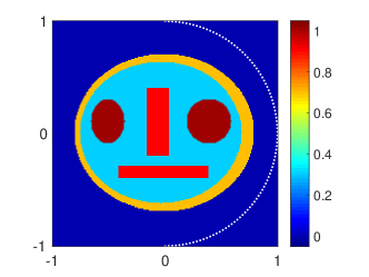
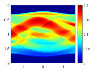
Figure 3.1: Left: The phantom ${\tt f}\in\mathbb{R}^{201\times 201}$ discretizing the head like function supported in a disc of radius 1. The white dots indicate locations of detectors. Right: The simulated discrete circular Radon transform ${\tt g}\in\mathbb{R}^{100\times 201}$. The horizontal axis is the detector location in $[-\pi/2,\pi/2]$; the vertical axis the radius in $[0,2]$. Any partial data ${\tt g}_{i}\in\mathbb{R}^{1\times 201}$ corresponds to a column.

3.4 Numerical simulations

In the following numerical results we consider the case where $R=1$. We assume measurements on the half circle $\Gamma=\{(\boldsymbol{z}_{1},\boldsymbol{z}_{2})\in\mathbb{S}^{1}\mid\boldsymbol{z}_{2}>0\}$, choose $N_{x}=N_{r}=200$ and use $N=100$ detector locations on $\Gamma$. Further, we use a partition of $\Gamma$ in 100 arcs $\Gamma_{i}$ of equal arc length (i.e. $n=100$). The phantom ${\tt f}\in\mathbb{R}^{201\times 201}$ used for the presented results and the numerically computed data $\boldsymbol{\tt{M}}_{i}{\tt f}\in\mathbb{R}^{1\times 201}$ for $i=1,\dots,100$ are shown Figure 3.1. We refer to one cycle of the iterative methods after we performed an update using any of the equation. One such cycle consists of $n$ consecutive iterative updates for the AVEK and the Kaczmarz iteration and one iterative update for the Landweber iteration. The numerical effort for one cycle in any of the considered methods is given by $\mathcal{O}(NN_{x}^{2})$, with similar leading constants. For a fair comparison of step sizes, we rescale any of the operators $\mathbf{M}_{i}$ and $\mathbf{M}$ in such a way that $\left\|\mathbf{M}_{i}\right\|\simeq\left\|\mathbf{M}\right\|\simeq 1$ for $i=1,\dots,100$. Further, in the Kaczmarz and the AVEK method the equations are randomly rearranged prior to each cycle. We empirically observed that this accelerates the convergence of both methods.

Results for exact data

We first consider the case of exact data shown in Figure 3.1. The step sizes for Landweber, Kaczmarz and AVEK are chosen constant and at different values. The convergence behavior during the first 80 cycles is shown in Figure 3.2. As can be seen, the Landweber is the slowest and the Kaczmarz and the AVEK are comparably fast under suitable choice of step sizes. Note that although our convergence analysis of AVEK assumes a step size below 1, the AVEK method allows for a rather wide range of step sizes (up to 30 for this example), and that larger step sizes turn out to be stable and yield faster convergence. This is not the case for the Landweber and the Kaczmarz method, where a step size above 3 yields divergence.

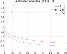
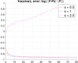
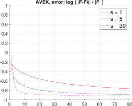
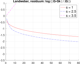
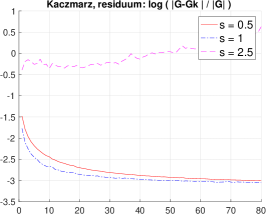
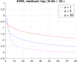
Figure 3.2: Residuum and relative reconstruction error (after taking logarithm to basis 10) of Landweber, Kaczmarz and AVEK with different step sizes for exact data during the first 80 cycles.

In order to visually compare the results, we choose proper step sizes for all methods in the sense that the iterations are fast and on the other hand stable. More precisely, for the Landweber iteration the step size has been taken as $s_{\rm LW}=2.5$, for the Kaczmarz iteration as $s_{\rm K}=1$ and for the AVEK as $s_{\rm AVEK}=30$. In Figure 3.3 we show reconstructions using the three considered methods after 10, 20 and 80 iterations. In any case, one notes reconstruction artifacts outside the convex hull of the detection curve, which is expected using limited view data [2, 18, 36, 46]. Inside the convex hull, the Kaczmarz and the AVEK give quite accurate results already after a reasonable number of cycles.

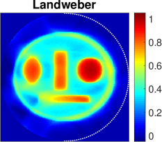
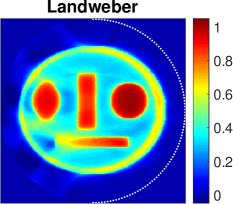
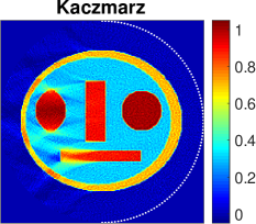
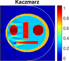
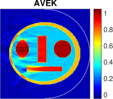
Figure 3.3: Reconstructions by Landweber, Kaczmarz and AVEK with proper choice of step sizes from exact data after 10 cycles (left column), 20 cycles (center column) and 80 cycles (right column).

Results for noisy data

We also tested the iterations on data ${\tt g}^{\delta}$ after adding $5\%$ noise. For that purpose added Gaussian white noise to ${\tt g}^{\delta}$ such that the resulting data satisfy $\|{\tt g}^{\delta}-{\tt g}\|/\|{\tt g}\|\simeq 0.05$. Different step sizes are taken for each method as in the exact data case and $\tau_{i}$ are chosen in such a way that no iterations are skipped. The convergence behavior during the first 80 cycles using noisy data is shown in Figure 3.4. The Kaczmarz method is the fastest, followed by the AVEK method, and the Landweber method is again the slowest. As in the exact data case, the AVEK iteration allows for way larger step sizes than the other two methods. Further, if step sizes are sufficiently small, the residuals $\|\mathbf{M}{\tt f}_{k}^{\delta}-{\tt g}^{\delta}\|$ are decreasing for all methods, while the reconstruction errors $\|{\tt f}_{k}^{\delta}-{\tt f}\|$ show the typical semi-convergence behavior for ill-posed problems. Interestingly, we point out that, in sharp contrast to the exact data case, iterations with small step sizes may outperform those with large step sizes. In noisy data case, slower convergence may provide smaller minimal reconstruction errors and further yields higher robustness in the choice of the iteration number as regularization parameter.

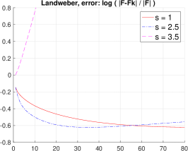
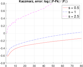
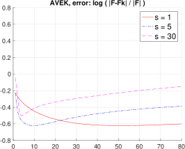
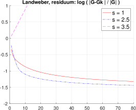
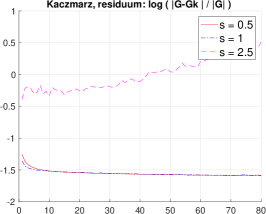
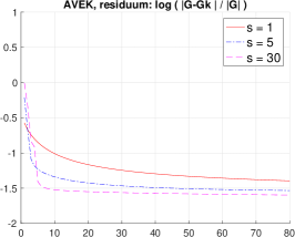
Figure 3.4: Residuum and relative reconstruction error (after taking logarithm to basis 10) of Landweber, Kaczmarz and AVEK with different step sizes for noisy data during the first 80 cycles.

For comparison of visual quality, we choose the empirically best step sizes for all methods; namely, $s_{\rm LW}=2.5$ for the Landweber iteration, $s_{\rm K}=1$ for the Kaczmarz iteration and $s_{\rm AVEK}=5$ for the AVEK iteration. The minimal $L^{2}$-reconstruction errors have been obtained after 35 iterations for the Landweber iteration, after 2 cycles for the Kaczmarz iteration, and after 10 cycles for the AVEK. The corresponding relative reconstruction errors $\|{\tt f}_{k}^{\delta}-{\tt f}\|/\|{\tt f}\|$ are $0.0595$ for the Kaczmarz method and $0.0571$ for the Landweber as well as the AVEK method. The Landweber and the AVEK method therefore slightly outperform the Kaczmarz method in terms of the minimal reconstruction error. Reconstruction results after 2, 10 and 35 iterations are shown in Figure 3.5. Further, through extensive simulations (not shown here), we find that the choice $s_{\rm AVEK}=5$ for the AVEK method is robust to different noise levels, which is thus recommended as the default step size for noisy data in practice.

In summary, from the simulations with exact and with noisy data, we conclude that the AVEK method is as comparably fast as the Kaczmarz method, and is meanwhile surprisingly stable with respect to the choice of step sizes. Such favorable properties are also observed for other data sets and are highly valuable in a great many of applications.

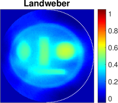
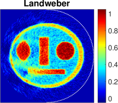
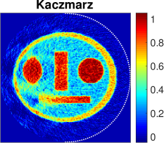
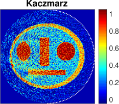
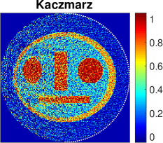
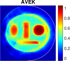
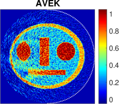
Figure 3.5: Reconstructions by Landweber, Kaczmarz and AVEK with proper choice of step sizes from noisy data after 2 cycles (left), 10 cycles (center) and 35 cycles (right).

3.5 Comparison with other methods

We further investigate the performance of the proposed AVEK method by comparing it with state-of-the-art accelerated versions of the Landweber and the Kaczmarz method proposed in [38]; compare also [13, 37, 39]. These accelerated methods take the same forms as the basic Landweber and the Kaczmarz method, with the only difference lying in the choice of step sizes; they select step sizes at each iteration via error minimizing relaxation (EMR) strategies. More precisely, the step size for the $k$-th iterative update is chosen to minimize $\langle\boldsymbol{f}^{\delta}_{k}-\boldsymbol{f},(\mathbf{M}^{*}\mathbf{M})^{s}(\boldsymbol{f}^{\delta}_{k}-\boldsymbol{f})\rangle$ in case of the Landweber method, and to minimize $\langle\boldsymbol{f}^{\delta}_{k}-\boldsymbol{f},(\mathbf{M}_{[k]}^{*}\mathbf{M}_{[k]})^{s}(\boldsymbol{f}^{\delta}_{k}-\boldsymbol{f})\rangle$ in case of the Kaczmarz method, for fixed $s\in\mathbb{N}_{0}$ (see [38] for details). We denote the resulting accelerated versions by Landweber-EMR and Kaczmarz-EMR, respectively. Additionally, we consider the incremental aggregated gradient (IAG) method [7], being closely related to the AVEK method, which is defined as

$$\boldsymbol{f}_{k+1}^{\delta}=\boldsymbol{f}_{k}^{\delta}-\frac{s_{k}}{n}\sum_{\ell=k-n+1}^{k}\mathbf{M}_{[\ell]}^{*}(\mathbf{M}_{[\ell]}(\boldsymbol{f}^{\delta}_{\ell})-\boldsymbol{g}^{\delta}_{[\ell]})\qquad\text{ for }k\geq n.$$

See (4.1) for the definition in case of general (possibly nonlinear) problems. We consider the same setting as in Section 3.4. In numerical simulations, parameter $s$ is set to $0$ or $1$ for the Landweber-EMR and the Kaczmarz-EMR method; the step sizes for the AVEK method are chosen the same as earlier (i.e. $s_{\rm AVEK}=30$ for exact data and $s_{\rm AVEK}=5$ for noisy data); the step size for IAG is chosen as $s_{\rm IAG}=0.08$ for exact data and $s_{\rm IAG}=0.06$ for noisy data, which leads to the best empirical performance. Moreover, for all methods the equations have been randomly rearranged prior to each cycle, which empirically accelerates the convergence.

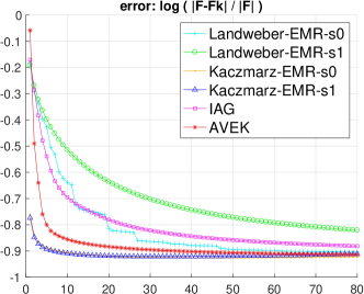
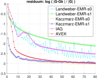
Figure 3.6: Residuum and relative reconstruction error (after taking logarithm to basis 10) of Landweber-EMR ($s=0$ or $1$), Kaczmarz-EMR ($s=0$ or $1$), IAG and AVEK for exact data during the first 80 cycles.

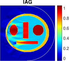
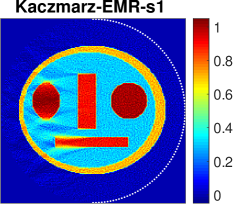
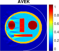
Figure 3.7: Reconstructions by Landweber-EMR ($s=0$ or $1$), Kaczmarz-EMR ($s=0$ and $1$), IAG and AVEK from exact data after 80 cycles.

For exact data the comparison of convergence behavior is illustrated in Figure 3.6. It shows that the two Kaczmarz-EMR methods are the fastest, closely followed by the AVEK, then the IAG and the Landweber-EMR ($s=1$), while the Landweber-EMR ($s=0$) is the slowest. Both the AVEK and the Kaczmarz-EMR methods obtain the smallest relative reconstruction errors and the smallest residuals among all methods. By comparing with Figure 3.2, one notes that the EMR strategies indeed accelerate the original Landweber and Kaczmarz methods for the circular Radon transform in terms of convergence rates. Further, notice that AVEK converges faster than IAG. Figure 3.7 gives a visual inspection of the convergence behavior for all methods.

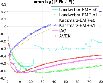
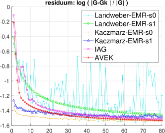
Figure 3.8: Residuum and relative reconstruction error (after taking logarithm to basis 10) of Landweber-EMR ($s=0$ or $1$), Kaczmarz-EMR ($s=0$ or $1$), IAG and AVEK for noisy data during the first 80 cycles.

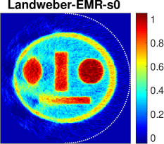
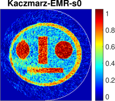
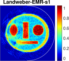
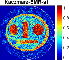
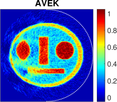
Figure 3.9: Reconstructions by Landweber-EMR ($s=0$ or $1$), Kaczmarz-EMR ($s=0$ or $1$), IAG and AVEK from noisy data at the cycles with minimal $L^{2}$-reconstruction errors.

The comparison for noisy data is summarized in Figure 3.8. In terms of relative reconstruction errors (which for inverse problems are more important than residuals), the AVEK performs the best, the IAG and the Landweber-EMR ($s=0$) rank second, followed by the Landweber-EMR ($s=1$). Unlike in the exact data case, the Kaczmarz-EMR methods are less satisfactory. This indicates that the convergence speed should not be the only concern for iterative methods if they are applied as regularization methods (cf. also Figure 3.4). The minimal relative reconstruction errors are achieved after 10 cycles for the AVEK, after 11 iterations for the Landweber-EMR ($s=0$), after 14 cycles for the IAG, after 30 iterations for the Landweber-EMR ($s=1$), and after 1 cycle for the Kaczmarz-EMR methods. The reconstructions with minimal reconstruction errors for all methods are shown in Figure 3.9.

As we have already noticed, developing appropriate step size strategies can significantly improve the results (see also [10]). Here we have simply used constant and conservative step sizes for the AVEK method. Further, adjusting the skipping parameters $\alpha_{k}$ can potentially improve and stabilize the AVEK method. A precise comparison of the methods using parameter fine-tuning and implementing adaptive and data-driven choices deserves further investigation; this, however, is beyond the scope of this paper.

4 Conclusion and outlook

In this paper we introduced the averaged Kaczmarz (AVEK) method as a paradigm of a new iterative regularization method. AVEK can be seen as a hybrid between Landweber’s and Kaczmarz’s method for solving inverse problems given as systems of equations $\mathbf{F}_{i}(\boldsymbol{x})=\boldsymbol{y}_{i}$. As the Kaczmarz method, AVEK requires only solving one forward and one adjoint problem per iteration. As the Landweber method, it uses information from all equations per update which can have a stabilizing effect. As main theoretical results, we have shown that the AVEK method converges weakly in the case of exact data (see Theorem 2.7), and presented convergence results for noisy data (see Theorem 2.10). Note that the convergence as $\delta\to 0$ in Theorem 2.10 (b) assumes strong convergence in the exact data case. It is an open problem if the same conclusion holds under its weak convergence only. Another open problem is the strong convergence for exact data in the general case. We conjecture both issues to hold true. Finally, it is of also interest to investigate the AVEK method (1.4)-(1.6) for general convex combinations with weights $\omega_{i}$ instead of equal weights $\omega_{i}=1/n$.

In Section 3, we presented numerical results for the AVEK method applied to the limited view problem for the circular Radon, which is relevant for photoacoustic tomography. For comparison purpose we also applied the Landweber and the Kaczmarz method to the same problem. In the exact data case, the observed convergence speed (number of cycles versus reconstruction error) of the AVEK turned out to be somewhere between the Kaczmarz (fastest) and the Landweber method (slowest). A similar behavior has been observed in the noisy data case. In this case, the minimal reconstruction error for the AVEK is slightly smaller that the one of the Kaczmarz method and equal to the Landweber method. The required number of iterations however is less than the one of the Landweber method. These initial results are encouraging and show that the AVEK is a useful iterative method for tomographic image reconstruction. Detailed studies are required in future work on the optimal selection of parameter such as the step sizes or the number of partitions. The increased stability of AVEK in terms of step sizes is worthy of further theoretical studies. Additionally, application of AVEK for non-linear inverse problems is another possible line of future research.

We see AVEK as the basic member of a new class of iterative reconstruction method. It shares some similarities with the incremental gradient method proposed in the seminal work [7] (studied for well-posed problems in finite dimensions). Applied to (1.1), the incremental gradient method reads

$$\forall k\geq n\colon\quad\boldsymbol{x}_{k+1}=\boldsymbol{x}_{k}-\frac{s_{k}}{n}\sum_{\ell=k-n+1}^{k}\mathbf{F}_{[\ell]}^{\prime}(\boldsymbol{x}_{\ell})^{*}(\mathbf{F}_{[\ell]}(\boldsymbol{x}_{\ell})-\boldsymbol{y}_{[\ell]})\,.$$ (4.1)

Instead of an average over individual auxiliary updates, the incremental gradient method uses an average over the individual gradients. Studying and analyzing the incremental gradient method for inverse problems is an interesting open issue. The incremental gradient method has been generalized in various directions. This includes proximal incremental gradient methods [5] or the averaged stochastic gradient method of [44]. Similar extensions for the AVEK (for ill-posed as well as well-posed problems) are interesting lines of future research.

Appendix A Deconvolution of sequences and proof of Lemma 2.5

The main aim of this appendix is to prove Lemma 2.5, concerning the convergence of the difference of two consecutive iterates of the AVEK iteration. For that purpose, we will first derive auxiliary results concerning deconvolution equations for sequences in Hilbert spaces that are of interest in its own.

For the following it is helpful to identify any sequence $(a_{k})_{k\in\mathbb{N}_{0}}\in\mathbb{C}^{\mathbb{N}_{0}}$ with a formal power series $a=\sum_{k=0}^{\infty}a_{k}X^{k}$. Here $X^{k}\in\mathbb{C}^{\mathbb{N}_{0}}$ is the sequence defined by $X^{k}_{k}=1$ and $X^{k}_{\ell}=0$ for $\ell\neq k$. For two complex sequences $a,b\in\mathbb{C}^{\mathbb{N}_{0}}$, the Cauchy product $a\ast b\in\mathbb{C}^{\mathbb{N}_{0}}$ is defined by $(a\ast b)_{k}\coloneqq\sum_{j=0}^{k}a_{j}b_{k-j}$; see [22]. We say that $a\in\mathbb{C}^{\mathbb{N}_{0}}$ is invertible if there is $b\in\mathbb{C}^{\mathbb{N}_{0}}$ with $a\ast b=(1,0,\dots)$. We write $b\coloneqq a^{-1}$ and call it the reciprocal formal power series of $a$, or simply the inverse of $a$. Moreover one easily verifies (see [22]) that the formal power series $a=\sum_{k=0}^{\infty}a_{k}X^{k}$ is invertible if and only if $a_{0}\neq 0$. In this case $b=a^{-1}$ is unique and defined by the recursion $b_{0}=1/a_{0}$ and $b_{k}=-\frac{1}{a_{0}}\sum_{j=0}^{k-1}b_{j}a_{k-j}$ for $k\geq 1$. One further verifies that $\mathbb{C}^{\mathbb{N}_{0}}$ together with point-wise addition and scalar multiplication and the Cauchy product forms an associative algebra.

A.1 Convolutions in Hilbert spaces

Throughout this subsection $\mathbb{X}$ denotes an arbitrary Hilbert space. For $a\in\mathbb{C}^{\mathbb{N}_{0}}$ and $\boldsymbol{x}\in\mathbb{X}^{\mathbb{N}_{0}}$ define the convolution $\boldsymbol{x}\ast a\in\mathbb{X}^{\mathbb{N}_{0}}$ by

$$\forall k\in{\mathbb{N}_{0}}\colon\quad(\boldsymbol{x}\ast a)_{k}\coloneqq\sum_{j=0}^{k}\boldsymbol{x}_{j}a_{k-j}\,.$$

One verifies that $(\boldsymbol{x}\ast a)\ast b=\boldsymbol{x}\ast(a\ast b)$ for $a,b\in\mathbb{C}^{\mathbb{N}_{0}}$ and $\boldsymbol{x}\in\mathbb{X}^{\mathbb{N}_{0}}$. Moreover, the set of bounded sequences $\ell^{\infty}({\mathbb{N}_{0}},\mathbb{X})\coloneqq\{\boldsymbol{x}\in\mathbb{X}^{\mathbb{N}_{0}}\mid\boldsymbol{x}_{k}\text{ bounded}\}$ forms a Banach space together with the uniform norm $\|x\|_{\infty}\coloneqq\sup\{\|\boldsymbol{x}_{k}\|\mid k\in{\mathbb{N}_{0}}\}$. Finally, $c_{0}({\mathbb{N}_{0}},\mathbb{X})\coloneqq\{\boldsymbol{x}\in\mathbb{X}^{\mathbb{N}_{0}}\mid\lim_{k\to\infty}\boldsymbol{x}_{k}=0\}$ denotes the space of sequences in $\mathbb{X}$ converging to zero, and $\ell^{1}({\mathbb{N}_{0}},\mathbb{C})\coloneqq\{\boldsymbol{x}\in\mathbb{X}^{\mathbb{N}_{0}}\mid\sum_{k=0}^{\infty}\left|\boldsymbol{x}_{k}\right|<\infty\}$ the space of summable sequences.

Lemma A.1.

Let $b\in\ell^{1}({\mathbb{N}_{0}},\mathbb{C})$ and define $b^{(m)}\coloneqq(b_{0},\dots,b_{m},0,\dots)$. Then,

1. $\forall\boldsymbol{x}\in c_{0}({\mathbb{N}_{0}},\mathbb{X})\colon\boldsymbol{x}\ast b^{(m)}\in c_{0}({\mathbb{N}_{0}},\mathbb{X})$;

2. $\forall\boldsymbol{x}\in\ell^{\infty}({\mathbb{N}_{0}},\mathbb{X})\colon\boldsymbol{x}\ast b\in\ell^{\infty}({\mathbb{N}_{0}},\mathbb{X})\wedge\lim_{m\to\infty}\|\boldsymbol{x}\ast b-\boldsymbol{x}\ast b^{(m)}\|_{\infty}=0$;

3. $\forall\boldsymbol{x}\in c_{0}({\mathbb{N}_{0}},\mathbb{X})\colon\boldsymbol{x}\ast b\in c_{0}({\mathbb{N}_{0}},\mathbb{X})$.

Proof.

(a) For $k\geq m$ we have $(\boldsymbol{x}\ast b^{(m)})_{k}=\sum_{j=0}^{k}\boldsymbol{x}_{j}b_{k-j}=\sum_{j=k-m}^{k}\boldsymbol{x}_{j}b_{k-j}$. Hence $\boldsymbol{x}\ast b^{(m)}$ converges to zero because $\boldsymbol{x}_{j}b_{k-j}$ does so.

(b) For $k\leq m$ we have $(\boldsymbol{x}\ast b^{(m)})_{k}=\sum_{j=0}^{k}\boldsymbol{x}_{j}b_{k-j}=(\boldsymbol{x}\ast b)_{k}$. For $k>m$ we have

• $(\boldsymbol{x}\ast b)_{k}-(\boldsymbol{x}\ast b^{(m)})_{k}=\sum_{j=0}^{k}\boldsymbol{x}_{j}b_{k-j}-\sum_{j=k-m}^{k}\boldsymbol{x}_{j}b_{k-j}=\sum_{j=0}^{k-m-1}\boldsymbol{x}_{j}b_{k-j}$;

• $\|(\boldsymbol{x}\ast b)_{k}-(\boldsymbol{x}\ast b^{(m)})_{k}\|\leq\left\|x\right\|_{\infty}\sum_{j=0}^{k-m-1}\left|b_{k-j}\right|\leq\|x\|_{\infty}\sum_{j=m+1}^{\infty}\left|b_{j}\right|$;

• $\sum_{j=m+1}^{\infty}\left|b_{j}\right|\to 0$ (because $\sum_{k\in{\mathbb{N}_{0}}}\left|b_{k}\right|<\infty$).

We conclude that $\|(\boldsymbol{x}\ast b)-(\boldsymbol{x}\ast b^{(m)})\|_{\infty}\leq\|x\|_{\infty}\sum_{j=m+1}^{\infty}\left|b_{j}\right|\to 0$.

(c) Follows from (a), (b) and the closedness of $c_{0}({\mathbb{N}_{0}},\mathbb{X})$ in $\ell^{\infty}({\mathbb{N}_{0}},\mathbb{X})$. ∎

As an application of Lemma A.1 we can show the following result, which is the main ingredient for the proof of Lemma 2.5.

Proposition A.2 (A deconvolution problem).

For any sequence $\boldsymbol{d}=(\boldsymbol{d}_{k})_{k=1}^{\infty}$ in $\mathbb{X}^{\mathbb{N}_{0}}$ and any $n\in{\mathbb{N}_{0}}$, the following implication holds true:

$$\lim_{k\to\infty}\sum_{j=1}^{n}j\boldsymbol{d}_{k-n+j}=0\implies\lim_{k\to\infty}\boldsymbol{d}_{k}=0\,.$$

Proof.

Set $a\coloneqq(n,n-1,\dots,1,0,\dots)$ and suppose that $(\boldsymbol{d}\ast a)_{k}\to 0$ as $k\to\infty$. We have to verify that $\boldsymbol{d}_{k}\to 0$ as $k\to\infty$, which is divided in several steps.

• Step 1: All zeros of the polynomial $p\colon\mathbb{C}\to\mathbb{C}\colon z\mapsto n+(n-1)z+\cdots z^{n-1}$ are contained in $\left\{z\in\mathbb{C}\mid\|z\|>1\right\}$.

  Because $p(0)\neq 0$, in order to verify Step 1, it is sufficient to show that all zeros of $p(1/z)$ are contained in the unit disc $B_{1}(0)=\left\{z\in\mathbb{C}\mid\|z\|<1\right\}$. Hence it is sufficient to show that the polynomial $q(z)\coloneqq z^{n-1}p(1/z)\coloneqq nz^{n-1}+(n-1)z^{n-2}+\cdots+1$ has all zeros in $B_{1}(0)$. Further note that $q(z)=Q^{\prime}(z)$, where $Q(z)\coloneqq z^{n}+z^{n-1}+\cdots+z$ has the form $Q(z)=z\frac{z^{n}-1}{z-1}$. Consequently, $\left\{0\right\}\cup\left\{z\in\mathbb{C}\mid z^{n}=1\wedge z\neq 1\right\}$ is the set of zeros of $Q$. The Gauss-Lukas theorem (see [33, Theorem (6,1)]) states that all critical points of a non-constant polynomial $f$ are contained in the convex hull $H$ of the set of zeros of $f$. If the zeros of $f$ are not collinear, then no critical point lies on $\partial H$ unless it is a multiple zero of $f$. Note that all zeros of $Q$ are simple, not collinear and contained in $\overline{B_{1}(0)}$. According the Gauss-Lukas theorem all zeros of $q=Q^{\prime}$ are contained in $B_{1}(0)$. Consequently all zeros of $p$ are indeed contained in $\{z\in\mathbb{C}\mid\|z\|>1\}$.

• Step 2: We have $a^{-1}\in\ell^{1}(\mathbb{N}_{0},\mathbb{C})$.

  All zeros of $p(z)$ are outside of $B_{1+\epsilon}(0)$ for some $\epsilon>0$ and therefore $1/p(z)$ is analytic in $B_{1+\epsilon}(0)$ and can be expanded in a power series $1/p(z)=\sum_{k\in\mathbb{N}_{0}}b_{k}z^{k}$. The radius of convergence is at least $1+\epsilon$ (as the radius of convergence of a function $f$ is the radius of the largest disc where $f$ or an analytic continuation of $f$ is analytic; see for example [22, Theorem 3.3a].) We have

  $$1=p(z)\frac{1}{p(z)}=\sum_{j=0}^{n-1}a_{j}z^{j}\sum_{k\in\mathbb{N}_{0}}b_{k}z^{k}=\sum_{k\in\mathbb{N}_{0}}(a\ast b)_{k}z^{k}\,.$$

  Hence $a\ast b=(1,0,0,\dots)$ and $a^{-1}=b\in\ell^{1}(\mathbb{N}_{0},\mathbb{C})$.

• Step 3: We are now ready to complete the proof. According to the assumption, we have $\boldsymbol{d}\ast a\in c_{0}(\mathbb{N}_{0},\mathbb{X})$. According to Step 2, we have $a^{-1}\in\ell^{1}(\mathbb{N}_{0},\mathbb{C})$. Therefore Lemma A.1 (c) implies that $\boldsymbol{d}=(\boldsymbol{d}\ast a)\ast a^{-1}\in c_{0}(\mathbb{N}_{0},\mathbb{X})$.

∎

A.2 Application to the AVEK iteration

Now let $\boldsymbol{x}_{k}$ be defined by (2.4), let $\boldsymbol{x}^{*}\in B_{\rho}(\boldsymbol{x}_{0})$ be an arbitrary solution to (1.1) and assume that (2.1) and (2.2) hold true. We introduce the auxiliary sequences $\boldsymbol{d}_{k}\coloneqq\boldsymbol{x}_{k+1}-\boldsymbol{x}_{k}$, $\boldsymbol{z}_{k}\coloneqq\frac{1}{n}\sum_{j=1}^{n}j\boldsymbol{x}_{k-n+j}$ and $\boldsymbol{r}_{k}\coloneqq\mathbf{F}_{[k]}^{\prime}(\boldsymbol{x}_{k})^{*}(\mathbf{F}_{[k]}(\boldsymbol{x}_{k})-\boldsymbol{y}_{[k]})$. Here $\boldsymbol{d}_{k}$ are the differences between two consecutive iterations that we show to converge to zero, $\boldsymbol{z}_{k}$ will be required in the subsequent analysis, and $\boldsymbol{r}_{k}$ are the residuals.

Lemma A.3.

1. $\lim_{k\to\infty}\boldsymbol{x}_{k+1}-{1}/{n}\sum_{l=k-n+1}^{k}\boldsymbol{x}_{\ell}=0$;

2. $\boldsymbol{z}_{k+1}-\boldsymbol{z}_{k}=\boldsymbol{x}_{k+1}-{1}/{n}\sum_{\ell=k-n+1}^{k}\boldsymbol{x}_{\ell}$;

3. $\lim_{k\to\infty}\boldsymbol{z}_{k+1}-\boldsymbol{z}_{k}={1}/{n}\lim_{k\to\infty}\sum_{j=1}^{n}j\boldsymbol{d}_{k-n+j}=0$.

Proof.

(a): By the definition of $\boldsymbol{x}_{k}$, $\boldsymbol{r}_{k}$ we have $\boldsymbol{x}_{k+1}=\frac{1}{n}\sum_{\ell=k-n+1}^{k}\boldsymbol{x}_{\ell}-s_{\ell}\boldsymbol{r}_{\ell}$. Therefore

$$\Bigl{\lVert}\boldsymbol{x}_{k+1}-\frac{1}{n}\sum_{l=k-n+1}^{k}\boldsymbol{x}_{\ell}\Bigr{\rVert}=\Bigl{\lVert}\frac{1}{n}\sum_{\ell=k-n+1}^{k}s_{\ell}\boldsymbol{r}_{\ell}\Bigr{\rVert}\leq\frac{1}{n}\sum_{\ell=k-n+1}^{k}s_{\ell}\|\boldsymbol{r}_{\ell}\|\,.$$

As we already know that $s_{\ell}\|\boldsymbol{r}_{\ell}\|\to 0$, the claim follows.

(b): We have

$$\boldsymbol{z}_{k+1}-\boldsymbol{z}_{k} =\frac{1}{n}\sum_{j=1}^{n}j\boldsymbol{x}_{k-n+j+1}-\frac{1}{n}\sum_{j=1}^{n}j\boldsymbol{x}_{k-n+j}$$

$$=\boldsymbol{x}_{n+1}+\frac{1}{n}\sum_{j=1}^{n-1}j\boldsymbol{x}_{k-n+j+1}-\frac{1}{n}\sum_{j=2}^{n}j\boldsymbol{x}_{k-n+j}-\frac{1}{n}\boldsymbol{x}_{k-n+1}$$

$$=\boldsymbol{x}_{n+1}+\frac{1}{n}\sum_{j=2}^{n}(j-1)\boldsymbol{x}_{k-n+j}-\frac{1}{n}\sum_{j=2}^{n}j\boldsymbol{x}_{k-n+j}-\frac{1}{n}\boldsymbol{x}_{k-n+1}$$

$$=\boldsymbol{x}_{n+1}-\frac{1}{n}\sum_{j=2}^{n}\boldsymbol{x}_{k-n+j}-\frac{1}{n}\boldsymbol{x}_{k-n+1}=\boldsymbol{x}_{n+1}-\frac{1}{n}\sum_{j=1}^{n}\boldsymbol{x}_{k-n+j}\,.$$

(c): Follows from (a), (b). ∎

Proof of Lemma 2.5

Lemma 2.5 now is an immediate consequence of Lemma A.3 and Proposition A.2. In fact, from Lemma A.3 (c) we know that $\lim_{k\to\infty}\sum_{j=1}^{n}j\boldsymbol{d}_{k-n+j}=0$ for $k\to\infty$. Then the assertion follows from Proposition A.2.

References

- [1] L.-E. Andersson, On the determination of a function from spherical averages, SIAM J. Appl. Math., 19 (1988), pp. 214–232.
- [2] L. L. Barannyk, J. Frikel, and L. V. Nguyen, On artifacts in limited data spherical Radon transform: curved observation surface, Inverse Probl., 32 (2016), pp. 015012, 32.
- [3] J. Baumeister, B. Kaltenbacher, and A. Leitao, On Levenberg-Marquardt-Kaczmarz iterative methods for solving systems of nonlinear ill-posed equations, Inverse Probl. Imaging, 4 (2010), pp. 335–350.
- [4] A. Beltukov and D. Feldman, Identities among Euclidean Sonar and Radon transforms, Adv. in Appl. Math., 42 (2009), pp. 23–41.
- [5] D. P. Bertsekas, Incremental proximal methods for large scale convex optimization, Math. Program., 129 (2011), pp. 163–195.
- [6] B. Blaschke, A. Neubauer, and O. Scherzer, On convergence rates for the iteratively regularized Gauss-Newton method, IMA J. Numer. Anal., 17 (1997), pp. 421–436.
- [7] D. Blatt, A. O. Hero, and H. Gauchman, A convergent incremental gradient method with a constant step size, SIAM J. Optim., 18 (2007), pp. 29–51.
- [8] N. Bleistein, J. K. Cohen, and J. W. Stockwell, Jr., Mathematics of multidimensional seismic imaging, migration, and inversion, vol. 13 of Interdisciplinary Applied Mathematics, Springer-Verlag, New York, 2001. Geophysics and Planetary Sciences.
- [9] P. Burgholzer, J. Bauer-Marschallinger, H. Grün, M. Haltmeier, and G. Paltauf, Temporal back-projection algorithms for photoacoustic tomography with integrating line detectors, Inverse Probl., 23 (2007), p. S65.
- [10] Y. Censor, P. P. B. Eggermont, and D. Gordon, Strong underrelaxation in Kaczmarz’s method for inconsistent systems, Numer. Math., 41 (1983), pp. 83–92.
- [11] G. Cimmino, Calcolo approssimato per le soluzioni dei sistemi di equazioni lineari, La Ricerca Scientifica, II (1938), pp. 326–333.
- [12] A. De Cezaro, M. Haltmeier, A. Leitão, and O. Scherzer, On steepest-descent-Kaczmarz methods for regularizing systems of nonlinear ill-posed equations, Appl. Math. Comput., 202 (2008), pp. 596–607.
- [13] L. T. Dos Santos, A parallel subgradient projections method for the convex feasibility problem, J. Comput. Appl. Math., 18 (1987), pp. 307–320.
- [14] H. Egger and A. Neubauer, Preconditioning Landweber iteration in Hilbert scales, Numer. Math., 101 (2005), pp. 643–662.
- [15] T. Elfving, P. C. Hansen, and T. Nikazad, Convergence analysis for column-action methods in image reconstruction, Numer. Algorithms, 74 (2017), pp. 905–924.
- [16] H. W. Engl, M. Hanke, and A. Neubauer, Regularization of inverse problems, vol. 375 of Mathematics and its Applications, Kluwer Academic Publishers Group, Dordrecht, 1996.
- [17] D. Finch, M. Haltmeier, and Rakesh, Inversion of spherical means and the wave equation in even dimensions, SIAM J. Appl. Math., 68 (2007), pp. 392–412.
- [18] J. Frikel and E. T. Quinto, Artifacts in incomplete data tomography with applications to photoacoustic tomography and sonar, SIAM J. Appl. Math., 75 (2015), pp. 703–725.
- [19] M. Haltmeier, R. Kowar, A. Leitão, and O. Scherzer, Kaczmarz methods for regularizing nonlinear ill-posed equations. II. Applications, Inverse Probl. Imaging, 1 (2007), pp. 507–523.
- [20] M. Haltmeier, A. Leitão, and O. Scherzer, Kaczmarz methods for regularizing nonlinear ill-posed equations. I. Convergence analysis, Inverse Probl. Imaging, 1 (2007), pp. 289–298.
- [21] M. Hanke, A. Neubauer, and O. Scherzer, A convergence analysis of the Landweber iteration for nonlinear ill-posed problems, Numer. Math., 72 (1995), pp. 21–37.
- [22] P. Henrici, Applied and computational complex analysis, vol. 1, Wiley-Interscience, New York-London-Sydney, 1974.
- [23] M. Jiang and G. Wang, Convergence studies on iterative algorithms for image reconstruction, IEEE Tran. Med. Imaging, 22 (2003), pp. 569–579.
- [24] B. Kaltenbacher, A. Neubauer, and O. Scherzer, Iterative regularization methods for nonlinear ill-posed problems, vol. 6 of Radon Series on Computational and Applied Mathematics, Walter de Gruyter GmbH & Co. KG, Berlin, 2008.
- [25] S. Kindermann and A. Leitão, Convergence rates for Kaczmarz-type regularization methods, Inverse Probl. Imaging, 8 (2014), pp. 149–172.
- [26] J. T. King and D. Chillingworth, Approximation of generalized inverses by iterated regularization, Numer. Funct. Anal. Optim., 1 (1979), pp. 499–513.
- [27] R. Kowar and O. Scherzer, Convergence analysis of a Landweber-Kaczmarz method for solving nonlinear ill-posed problems, in Ill-posed and inverse problems, VSP, Zeist, 2002, pp. 253–270.
- [28] P. Kuchment and L. Kunyansky, Mathematics of photoacoustic and thermoacoustic tomography, in Handbook of Mathematical Methods in Imaging, Springer, 2011, pp. 817–865.
- [29] L. Landweber, An iteration formula for Fredholm integral equations of the first kind, Amer. J. Math., 73 (1951), pp. 615–624.
- [30] L. J. Lardy, A series representation for the generalized inverse of a closed linear operator, Atti Accad. Naz. Lincei Rend. Cl. Sci. Fis. Mat. Natur. (8), 58 (1975), pp. 152–157.
- [31] A. Leitão and B. F. Svaiter, On projective Landweber-Kaczmarz methods for solving systems of nonlinear ill-posed equations, Inverse Probl., 32 (2016), pp. 025004, 20.
- [32] Z. Q. Luo, On the convergence of the lms algorithm with adaptive learning rate for linear feedforward networks, Neural Comput., 3 (1991), pp. 226–245.
- [33] M. Marden, Geometry of polynomials, Second edition. Mathematical Surveys, No. 3, American Mathematical Society, Providence, R.I., 1966.
- [34] F. Natterer and F. Wübbeling, Mathematical Methods in Image Reconstruction, vol. 5 of Monographs on Mathematical Modeling and Computation, SIAM, Philadelphia, PA, 2001.
- [35] A. Neubauer and O. Scherzer, A convergence rate result for a steepest descent method and a minimal error method for the solution of nonlinear ill-posed problems, Z. Anal. Anwendungen, 14 (1995), pp. 369–377.
- [36] L. V. Nguyen, On artifacts in limited data spherical Radon transform: flat observation surfaces, SIAM J. Math. Anal., 47 (2015), pp. 2984–3004.
- [37] T. Nikazad and M. Abbasi, An acceleration scheme for cyclic subgradient projections method, Comput. Optim. Appl., 54 (2013), pp. 77–91.
- [38] T. Nikazad, M. Abbasi, and T. Elfving, Error minimizing relaxation strategies in Landweber and Kaczmarz type iterations, J. Inverse Ill-Posed Probl., 25 (2017), pp. 35–56.
- [39] T. Nikazad, M. Abbasi, and M. Mirzapour, Convergence of string-averaging method for a class of operators, Optim. Methods Softw., 31 (2016), pp. 1189–1208.
- [40] S. J. Norton and M. Linzer, Ultrasonic reflectivity imaging in three dimensions: Exact inverse scattering solutions for plane, cylindrical and spherical apertures, IEEE Trans. Biomed. Eng., 28 (1981), pp. 202–220.
- [41] Z. a. Opial, Weak convergence of the sequence of successive approximations for nonexpansive mappings, Bull. Amer. Math. Soc., 73 (1967), pp. 591–597.
- [42] A. Rieder, On the regularization of nonlinear ill-posed problems via inexact Newton iterations, Inverse Probl., 15 (1999), pp. 309–327.
- [43] O. Scherzer, M. Grasmair, H. Grossauer, M. Haltmeier, and F. Lenzen, Variational methods in imaging, vol. 167 of Applied Mathematical Sciences, Springer, New York, 2009.
- [44] M. Schmidt, N. Le Roux, and F. Bach, Minimizing finite sums with the stochastic average gradient, Math. Program., 162 (2017), pp. 83–112.
- [45] M. V. Solodov, Incremental gradient algorithms with stepsizes bounded away from zero, Comput. Optim. Appl., 11 (1998), pp. 23–35.
- [46] P. Stefanov and G. Uhlmann, Is a curved flight path in SAR better than a straight one?, SIAM J. Appl. Math., 73 (2013), pp. 1596–1612.
- [47] K. Wang, R. W. Schoonover, R. Su, A. Oraevsky, and M. A. Anastasio, Discrete imaging models for three-dimensional optoacoustic tomography using radially symmetric expansion functions, IEEE Trans. Med. Imag., 33 (2014), pp. 1180–1193.
- [48] M. Xu and L. V. Wang, Universal back-projection algorithm for photoacoustic computed tomography, Phys. Rev. E, 71 (2005), p. 016706.
- [49] G. Zangerl, O. Scherzer, and M. Haltmeier, Exact series reconstruction in photoacoustic tomography with circular integrating detectors, Commun. Math. Sci., 7 (2009), pp. 665–678.