Numerical Homogenization of Heterogeneous Fractional Laplacians

Abstract

In this paper, we develop a numerical multiscale method to solve the fractional Laplacian with a heterogeneous diffusion coefficient. When the coefficient is heterogeneous, this adds to the computational costs. Moreover, the fractional Laplacian is a nonlocal operator in its standard form, however the Caffarelli-Silvestre extension allows for a localization of the equations. This adds a complexity of an extra spacial dimension and a singular/degenerate coefficient depending on the fractional order. Using a sub-grid correction method, we correct the basis functions in a natural weighted Sobolev space and show that these corrections are able to be truncated to design a computationally efficient scheme with optimal convergence rates. A key ingredient of this method is the use of quasi-interpolation operators to construct the fine scale spaces. Since the solution of the extended problem on the critical boundary is of main interest, we construct a projective quasi-interpolation that has both $d$ and $d+1$ dimensional averages over subsets in the spirit of the Scott-Zhang operator. We show that this operator satisfies local stability and local approximation properties in weighted Sobolev spaces. We further show that we can obtain a greater rate of convergence for sufficient smooth forces, and utilizing a global $L^{2}$ projection on the critical boundary. We present some numerical examples, utilizing our projective quasi-interpolation in dimension $2+1$ for analytic and heterogeneous cases to demonstrate the rates and effectiveness of the method.

Keywords: localization, multiscale methods, fractional Laplacian, heterogeneous diffusion

1 Introduction

In the modeling and simulation of porous media or composite materials, the multiscale nature of the materials is a challenging mathematical problem. In addition to this challenge, the modeling of non-local behavior that naturally occurs in particular media is of great interest, for example in the modeling of non-local mechanics [47], fractional (and thus non-local) Keller-Segel models of chemotaxis [48], and in ground water flow by fractional (non-Fickian) transport [21, 38]. The areas of multiscale problems and non-local fractional problems have significant overlap in these applications. In particular, it is well known in hydrology and reservoir engineering that the permeability of the subsurface is highly heterogeneous. The Macro-Dispersion Experiment (MADE) [45] demonstrated experimentally non-Darcy transport that exhibits non-local effects. The challenge of simulating these types of problems is two fold: 1) the heterogeneity of the subsurface properties creates the need for higher resolutions and 2) the non-locality effects the band structure of the linear solvers creating often dense matrices. In this work, we present a multiscale method to mitigate both issues of non-locality and the heterogeneous properties.

The model we will focus on in this work is the heterogeneous fractional Laplacian. This is the Darcy flow model with a multiscale permeability coefficient and a fractional derivative power to incorporate the non-local behavior. There is a vast literature on the analysis and simulation of the fractional Laplacian. Due to a relatively recent result of Caffarelli and Silvestre [15], the solution of the fractional Laplacian is more tractable in both terms of analysis and computation. By adding an extra spatial dimension, the fractional Laplacian is transformed into an weighted harmonic extension problem, or a singular/degenerate (depending on fractional degree) linear elliptic problem. The numerical solution of such problems has been approached by several authors in [42] using quasi-interpolation, in [6] using a novel integral representation formula, fractional equations are solved via a Petrov-Galerkin method in [32], and for tensor finite elements in [4], to name a few. A recent survey article of numerical methods for fractional diffusion equations in homogeneous media can be found in [5].

The new challenge to be addressed in this paper is the derivation of effective numerical methods for fractional diffusion in heterogeneous media. The application of numerical homogenization techniques has, to our knowledge, not been considered yet. The key idea of numerical homogenization being to incorporate scales on the fine-grid to the coarse-grid in a computationally feasible way. Several approaches exist to this end. The multiscale finite element method [30], where local basis functions are computed, the heterogeneous multiscale method [1], where local problems are solved to obtain coarse-grid coefficients, and the variational multiscale method [31], which is related to the technique we will use. We will employ the local orthogonal decomposition (LOD) method. The LOD method is a numerical homogenization method whereby the coarse-grid is augmented so that the corrections are localizable and truncated to design a computationally efficient scheme [29, 33, 37, 43]. This has been used successfully in many applications such as semi-linear problems [27], waves equations [2], perforated media [13], and diminishing the pollution in high-frequency problems [11, 12], to name a few.

A key component of this method is a quasi-interpolation operator that is utilized to construct a fine-scale space. The construction of such an operator for the fractional Laplacian is slightly more delicate due to the extra resolution one wants near the trace of the weighted extension problem. The authors in [42] utilize a quasi-interpolation based on regularized Taylor polynomials [10], which are a generalization of the Clément quasi-interpolation [18]. However, these quasi-interpolations are not projective. We proceed similar to [13], where the authors utilized a local $L^{2}$ projection onto the coarse-grid space, and prove local $L^{2}$ stability and approximabilty properties in weighted Sobolev spaces based on arguments in [7, 8]. For the weighted extension problem of the fractional Laplacian we would like to further resolve the information on the trace of the original domain. To this end, we develop a hybrid projective quasi-interpolation operator using techniques from [7, 46], whereby we use local $L^{2}$ projections for both $d$ and $d+1$ dimensional simplices to generate nodal values. With this quasi-interpolation, we prove the canonical convergence rate of $H^{s}$, $H$-coarse mesh size and $s$-fractional derivative degree, of the multiscale method on quasi-uniform meshes. Supposing more smoothness on the data and utilizing a slightly modified projection based on the gobal $L^{2}$ projection on the critical boundary, we are able to prove order $H$ convergence on the coarse-grid. We also prove the standard estimates with truncated corrections [27].

We present numerical results for two benchmark examples with the same forcing, but different diffusion coefficients, in the computational domain that is a subset of $\mathbb{R}^{2}\times(0,T)$. The first being a homogeneous problem of which has an analytic solution, and the second utilizing a heterogeneous coefficient from a $2-d$ slice of a standard benchmark problem. We show that we numerically obtain optimal rates of convergence in these examples once we pass the pre-asymptotic regime in terms of the truncation of the correctors. We compute solutions for various fractional orders $s$ above and below the critical fractional value of $s=\frac{1}{2}$.

This paper is organized as follows. We begin in Section 2 with the heterogeneous fractional Laplacian and the singular/degenerate elliptic problem of the Caffarelli-Silvestre extension. The weighted extension problem decays exponentially in the extended direction and thus can be truncated on a finite domain, this is the problem we shall focus on in this work. In Section 3, we define the relevant fractional Sobolev Spaces for completeness and develop the theory of weighted Sobolev Spaces critical to the setup and analysis of the Caffarelli-Silvestre extension. We also present various relevant weighted inequalities, such as the weighted Poincaré inequality. Then, in Section 4, we define the weighted quasi-interpolation operator that will be used to construct the LOD method. Local approximability and stability in the weighted spaces are proved. The multiscale method and related errors are introduced in Section 5. We then present two numerical examples in Section 6. Finally, the proofs for the truncation of correctors in weighted norms are given in the Appendix A.

2 Preliminaries

It is well known that fractional Laplacian problems are non-local. Therefore, applying standard two-grid techniques to handle heterogeneous coefficients locally is not possible as the sub-grid problems will too be non-local (in fact global). However, due to the Caffarelli-Silvestre extension [15], one is able to rewrite the non-local fractional Laplacian as a Dirichlet-to-Neumann mapping problem. This problem is localizable at the cost of a one dimension higher infinite domain and singular or degenerate coefficients depending on the fractional degree $s$. In this section we present the background on the fractional Laplace operator with a heterogeneous coefficient as well as the background on the Caffarelli-Silvestre extension problem.

2.1 Heterogeneous Fractional Laplacian

Let $\Omega\subset\mathbb{R}^{d}$ be a bounded, open, and connected Lipschitz domain for $d\geq 1$. We let ${\cal L}_{A}u=-\text{div}_{x}\left(A(x)\nabla_{x}u\right)$, where $A\in\left(L^{\infty}({\Omega})\right)^{d\times d}$ is assumed to be symmetric and satisfies for all $x\in{\Omega}$, $\xi\in\mathbb{R}^{d}$, and some $\alpha,\beta>0$

$$\alpha|\xi|^{2}\leq{\langle A(x)\xi,\xi\rangle}\leq\beta|\xi|^{2}.$$

We consider the following fractional Laplace equation with Dirichlet boundary condition, that is we seek a solution $u$ that satisfies for $s\in(0,1)$ and given data $f$:

$$\left({\cal L}_{A}u\right)^{s} =f\quad\text{in }{\Omega},$$ (1a)

$$u =0\quad\text{on }\partial{\Omega}.$$ (1b)

As shown in [16], one can write the heterogeneous fractional Laplacian (1) as

$$\left({\cal L}_{A}u\right)^{s}=\int_{\Omega}(u(x)-u(y))K_{s}(x,y)\,dy,$$ (2)

where $K_{s}(x,y)$ is the fundamental heat kernel to the operator ${\cal L}_{A}u$, and satisfies the bounds

$$0\lesssim K_{s}(x,y)\lesssim\frac{1}{|x-y|^{d+2s}},\,\,x\neq y.$$

In this work, we will write $a\lesssim b$, to mean that there exists a constant $C>0$ independent of the mesh parameters (but possibly depending on the domain, dimension, $s$, $\alpha$, $\beta$ but not on variations of $A$) such that $a\leq Cb$. Note that for the above integral formulation, one must compute the heat kernel for the heterogeneous operator which is computationally costly.

The fractional Laplacian operator may also be defined via the eigenfunctions of ${\cal L}_{A}$ given by

$$-\text{div}_{x}\left(A(x)\nabla_{x}\phi_{k}\right) =\mu_{k}\phi_{k}\quad\text{in }\Omega,$$ (3a)

$$\phi_{k} =0\quad\text{on }\partial\Omega,$$ (3b)

where the eigenpairs $(\mu_{k},\phi_{k})\in\mathbb{R}_{+}\times H^{1}_{0}(\Omega)$, for $k\in\mathbb{N}$, can be chosen such that $\{\phi_{k}\}_{k\in\mathbb{N}}$ form an orthonormal basis for $L^{2}(\Omega)$. Supposing $u\in\text{Dom}({\cal L}^{s}_{A})$, we expand $u$ as $u(x)=\sum_{k\in\mathbb{N}}u_{k}\phi_{k}(x)$, and define

$${\cal L}^{s}_{A}u=\sum_{k\in\mathbb{N}}\mu^{s}_{k}u_{k}\phi_{k},$$

where $u_{k}=\int_{\Omega}\phi_{k}u\,dx$.

2.2 Caffarelli-Silvestre Extension Problem

Using the formulation developed in [16, 42], we reformulate the fractional Laplacian problem (1) as an extension in ${\Omega}\times(0,\infty)\subset\mathbb{R}^{d+1}$. We denote the cylinder ${{\cal C}}={\Omega}\times(0,\infty)$, spatial variables $x\in\mathbb{R}^{d}$ and $y\in\mathbb{R}$, and the lateral boundary $\partial_{L}{{\cal C}}=\partial{\Omega}\times[0,\infty)$. We let $U=U(x,y):{{\cal C}}\to\mathbb{R}$, be a solution to the following singular/degenerate elliptic equation with coefficients $y^{\alpha}$:

$$-\text{div}\left(y^{a}B(x)\nabla U\right) =0\quad\text{in }{{\cal C}},$$ (4a)

$$\frac{\partial U}{\partial\nu^{a}}=-y^{a}\frac{\partial U}{\partial y}\Bigg{|}_{y=0} =c_{s}f(x)\quad\text{on }{\Omega},$$ (4b)

$$U =0\quad\text{on }\partial_{L}{{\cal C}}.$$ (4c)

The solution to (1) is given by $u(x)=U(x,0)$ for $x\in{\Omega}$.

Above, differential operators are given with respect to $x\in\mathbb{R}^{d}$ and $y\in\mathbb{R}$, i.e. $\nabla=(\nabla_{x},\partial_{y})^{T}$, and the tensor $B\in\mathbb{R}^{d+1}\times\mathbb{R}^{d+1}$ is given by

$$B(x)=\begin{bmatrix}A(x)&0_{d\times 1}\\ 0_{1\times d}&1\end{bmatrix},$$

for $a=1-2s\in(-1,1)$ or $s=\frac{a-1}{2}\in(0,1)$. We will often move freely between the fractional degree $s$ and the power of the weight $a$. Here, $\frac{\partial U}{\partial\nu^{a}}$ is the co-normal exterior derivative with outer unit normal $\nu$ and $c_{s}=2^{1-2s}\frac{\Gamma(1-s)}{\Gamma(s)}>0$ is a positive constant that solely depends on $s$.

We note that, supposing appropriate data $f$, $u$ is a solution of the heterogeneous fractional Laplacian (1) if and only if $U$ is a solution to the weighted harmonic extension (4). The solution to the weighted harmonic extension is related to the spectral representation of the solution of the fractional Laplace. We write $u(x)=\sum_{k\in\mathbb{N}}u_{k}\phi_{k}(x)$, where $\{\phi_{k}\}_{k\in\mathbb{N}}$ satisfy (3), then we have from [9, 17], that we may write

$$U(x,y)=\sum_{k\in\mathbb{N}}u_{k}\phi_{k}(x)\psi_{k}(y),$$

where $\psi_{k}(y)$ satisfies

$$\psi^{{}^{\prime\prime}}_{k}+\frac{a}{y}\psi^{\prime}_{k}-\mu_{k}\psi_{k}=0\text{ in }(0,\infty),$$

with the boundary conditions $\psi_{k}(0)=1,$ and $\lim_{y\to\infty}\psi_{k}(y)=0$, for all $k\in\mathbb{N}$. This above equation has a known solution from [14, 17], that is $\psi_{k}(y)=\exp(-\sqrt{\mu_{k}}y)$ if $s=\frac{1}{2}$ and $\psi_{k}(y)=C_{s}\left(\sqrt{\mu_{k}}y\right)^{s}K_{s}(\sqrt{\mu_{k}}y)$, for $s\in(0,1)\backslash\{\frac{1}{2}\}$, where $K_{s}$ is the modified Bessel function of second kind. Therefore the solution decreases exponentially in the $y$-direction, allowing to truncate the computational domain.

Remark 2.1.

Naturally, $f$ is in the dual-space $\mathbb{H}^{-s}(\Omega)$ of the fractional space $\mathbb{H}^{s}$ (to be defined more precisely in Section 3.1). However, we will often take $f$ to be more regular and suppose $f\in L^{2}(\Omega)$ or in $\mathbb{H}^{1-s}(\Omega)$ when the extra regularity is useful or needed for existence and uniqueness.

Remark 2.2.

We will further suppose that $f$ is compatible with the Dirichlet boundary condition c.f . [42, Remark 2.8]. In particular, we will suppose that in the regime $s\in(0,\frac{1}{2})$, the data vanishes sufficiently fast near $\partial\Omega$, in the regime $s\in(\frac{1}{2},1)$, $f\in\mathbb{H}^{1-s}(\Omega)$ is sufficient. The case $s=\frac{1}{2}$ is the non-weighted standard harmonic extension.

To facilitate the solution of (4) we need additional notation and properties of weighted Sobolev spaces, explored in great detail in [34]. For $x\in\mathbb{R}^{d}$ and $y\in\mathbb{R}_{+}$, we write ${\bf x}=(x,y)$ and let $d{\bf x}=dx\,dy$, be the standard tensor product Lebesgue measure on $\mathbb{R}^{d+1}$. For $\omega\subset\mathbb{R}^{d}\times\mathbb{R}_{+}$, an open set and $a:=1-2s\in(-1,1)$, we define $L^{2}(\omega,y^{a})$ to be all measurable functions $u$ on $\omega$ such that

$${\left\lVert u\right\rVert}_{L^{2}\left(\omega,y^{a}\right)}^{2}=\int_{\omega}u^{2}\,y^{a}\,d{\bf x}<\infty,$$

and define $H^{1}(\omega,y^{a})$ similarly, by all measurable functions $u$ on $\omega$ such that

$${\left\lVert u\right\rVert}_{H^{1}\left(\omega,y^{a}\right)}:=\left({\left\lVert u\right\rVert}_{L^{2}\left(\omega,y^{a}\right)}^{2}+{\left\lVert\nabla u\right\rVert}_{L^{2}\left(\omega,y^{a}\right)}^{2}\right)^{\frac{1}{2}}<\infty.$$

Finally, we define the space incorporating the homogeneous Dirichlet boundary condition on the outer cylinder as

$$\mathring{H}^{1}_{L}({{\cal C}},y^{a})=\{u\in H^{1}({{\cal C}},y^{a})\,:\,u=0\text{ on }\partial_{L}{{\cal C}}\}.$$

Integrating (4) by parts we obtain the following weak form: find $U\in\mathring{H}^{1}_{L}({{\cal C}},y^{a})$ such that

$$B(U,\psi)=F(\psi)\quad\text{for all }\psi\in\mathring{H}^{1}_{L}({{\cal C}},y^{a}),$$ (5)

where the bilinear and linear forms read

$$B(U,\psi):=\int_{{{\cal C}}}B(x)\nabla U\nabla\psi\,y^{a}\,d{\bf x}\qquad\textrm{and}\qquad F(\psi):=\int_{{\Omega}}c_{s}f(x)\psi(x,0)\,dx.$$

As the above problem is in an infinite domain, we introduce a truncated cylinder solution for computations, which is extend by zero to the infinite domain. We denote the truncated domain ${{\cal C}_{T}}={\Omega}\times(0,T)$, and $\partial_{L}{{\cal C}_{T}}=\left(\partial{\Omega}\times[0,T]\right)\cup\left(\Omega\times\{T\}\right)$, for some $T>0$. We have the related truncated space given by

$$\mathring{H}^{1}_{L}({{\cal C}_{T}},y^{a})=\{u\in H^{1}({{\cal C}_{T}},y^{a})\,:\,u=0\text{ on }\partial_{L}{{\cal C}_{T}}\}.$$

We then solve for $U_{T}\in\mathring{H}^{1}_{L}({{\cal C}_{T}},y^{a})$ such that

$$B_{T}(U_{T},\psi)=F(\psi)\quad\text{for all }\psi\in\mathring{H}^{1}_{L}({{\cal C}_{T}},y^{a}),$$ (6)

where we introduce the natural notation for the truncated bilinear form

$$B_{T}(U_{T},\psi):=\int_{{{\cal C}_{T}}}B(x)\nabla U_{T}\nabla\psi\,y^{a}\,d{\bf x}.$$

Extending $U_{T}$ by zero into ${{\cal C}}$ we may obtain an infinite domain approximation which we do not relabel. The following exponential error estimate was proven in [42, Lemma 3.3], which we restate here for completeness.

Theorem 2.3.

Let $T\geq 1$ and let $U$ be a solution to (5), and $U_{T}$ satisfy (6), for $f\in H^{-s}(\Omega)$, then we have

$${\left\lVert\nabla(U-U_{T})\right\rVert}_{L^{2}\left({{\cal C}},y^{a}\right)}\lesssim e^{-CT}\left\lVert f\right\rVert_{H^{-s}(\Omega)},$$

for $C>0$ independent of $T$.

Thus, the solution of the truncated problem will suffice for a sufficiently large $T$. In the remaining parts of this paper, we will merely consider the numerical approximation of $U_{T}$ extended by zero into ${{\cal C}}$. We will drop the truncation notation in the following sections, as well as the capital lettering $U$ for the solution to the weighted harmonic extension if there is no ambiguity.

Remark 2.4.

For a full discussion on the regularity and approximation of the fine-grid problem we refer again to [42, Section 2.6]. For our numerical homogenization method, we will not consider the fine-grid error and focus merely on the coarse-grid error.

3 Sobolev Spaces and Inequalities

In this section we will introduce the notation of fractional and weighted Sobolev spaces. First, we recall the results and notation of fractional and weighted Poincaré inequalities presented in [42] and references therein. We also present and prove some useful inverse and trace inequalities in the weighted Sobolev space, thus linking the two kinds of Sobolev spaces.

3.1 Fractional Sobolev Spaces

Here we recall some details of fractional Sobolev spaces as they will be related to the trace spaces of the weighted spaces we will consider, as well as being the natural space for the solution $u$ to (1). There is a vast literature on this subject and for details we refer to [22]. We loosely follow the presentation of [42] in the following. We begin by introducing the Gagliardo-Slobodeckij seminorm for $s\in(0,1)$:

$$|u|^{2}_{H^{s}(\Omega)}=\int_{\Omega}\int_{\Omega}\frac{|u(x)-u(x^{\prime})|^{2}}{|x-x^{\prime}|^{d+2s}}\,dx\,dx^{\prime},$$

and the related norm $\left\lVert u\right\rVert^{2}_{H^{s}(\Omega)}=\left\lVert u\right\rVert^{2}_{L^{2}(\Omega)}+|u|^{2}_{H^{s}(\Omega)}$. We define the Sobolev space $H^{s}(\Omega)$ to be the measurable functions such that $\left\lVert u\right\rVert_{H^{s}(\Omega)}<\infty$. For detailed construction we refer to [49]. We define the space $H^{s}_{0}(\Omega)$ to be the closure of $C_{0}^{\infty}(\Omega)$ with respect to the norm $\left\lVert\cdot\right\rVert_{H^{s}(\Omega)}$.

If the boundary of $\Omega$ is smooth enough, an interpolation space interpretation is possible [35]. We may write the Sobolev space with $s\in[0,1]$ and $\theta=1-s,$ as the interpolation space pair

$$H^{s}(\Omega)=\left[H^{1}(\Omega),L^{2}(\Omega)\right]_{\theta}\quad\text{and}\quad H^{s}_{0}(\Omega)=\left[H^{1}_{0}(\Omega),L^{2}(\Omega)\right]_{\theta},\quad\theta\neq\frac{1}{2}.$$

For the critical case $s=\frac{1}{2}$, this is the so called Lions-Magenes space

$$H^{\frac{1}{2}}_{00}(\Omega)=\left[H^{1}_{0}(\Omega),L^{2}(\Omega)\right]_{\frac{1}{2}},$$

this space satisfies

$$H^{\frac{1}{2}}_{00}(\Omega)=\Bigg{\{}u\in H^{\frac{1}{2}}(\Omega):\int_{\Omega}\frac{u^{2}(x)}{\text{dist}(x^{\prime},\partial\Omega)}\,dx^{\prime}<\infty\Bigg{\}}.$$

We summarize this in a general notation as

$$\mathbb{H}^{s}(\Omega)=\begin{cases}H^{s}(\Omega),&\text{ for }s\in(0,\frac{1}{2}),\\ H^{1/2}_{00}(\Omega),&\text{ for }s=\frac{1}{2},\\ H^{s}_{0}(\Omega),&\text{ for }s\in(\frac{1}{2},1).\end{cases}$$

3.2 Weighted Sobolev Spaces and Inequalities

We now give the background for weighted Sobolev spaces as well as present some critical inequalities. A key property of the weight $y^{a}$ is that it belongs the Muckenhoupt class $A_{2}(\mathbb{R}^{d+1})$ [25, 40]. For a general weight, $w\in L_{loc}^{1}(\mathbb{R}^{d+1})$, we say that $w\in A_{2}(\mathbb{R}^{d+1})$ if there exists a $C_{2,w}>0$ such that

$$\sup_{B}\left(\frac{1}{|B|}\int_{B}w\,d{\bf x}\right)\left(\frac{1}{|B|}\int_{B}w^{-1}\,d{\bf x}\right)=C_{2,w}<\infty,$$ (7)

for all balls $B\subset\mathbb{R}^{d+1}.$ We will denote the Muckenhoupt weight constant for $y^{a}$ as $C_{2,a}$. We will now give a few of the critical inequalities and properties related to this class of weighted Sobolev spaces.

A key inequality for the analysis is the weighted Poincaré inequality. The weighted Poincaré inequality for Muckenhoupt weights is well studied in nonlinear potential theory of degenerate problems [24, 26] and references therein. We will state the result here without proof.

Lemma 3.1 (Weighted Poincaré Inequality).

Let $\omega\subset\Omega\times(0,\infty)$, be a bounded, star-shaped domain (with respect to the ball B) and $\text{diam}(\omega)\approx H$. If $w\in H^{1}(\omega,y^{a})$ it holds that

$$\left\lVert w-{\langle w\rangle}_{\omega}\right\rVert_{L^{2}(\omega,y^{a})}\lesssim H\left\lVert\nabla w\right\rVert_{L^{2}(\omega,y^{a})},$$ (8)

where the constants are independent of $H$ and ${\langle w\rangle}_{\omega}=\frac{1}{|\omega|}\int_{\omega}w\,d{\bf x}$. ∎

Remark 3.2.

Note that the above inequality may be extended to a connected union of star-shaped domains where the average can be taken over a subdomain [42, Corollary 4.4]. We will refer to both of these results simply as the Weighted Poincaré Inequality when there is no ambiguity.

We have the following $L^{\infty}\to L^{2}$ weighted inverse inequality. For this we suppose that we have a coarse quasi-uniform, shape-regular, discretization ${\cal T}_{{{\cal C}_{T}}}$ of the domain ${{\cal C}_{T}}$ with characteristic mesh size $H$. Similarly, we denote the restricted mesh onto the lower dimensional space $\Omega$, to be ${\cal T}_{\Omega}$. We denote by $\mathbb{P}_{1}(T)$ the linear polynomials on $T\in{\cal T}_{{{\cal C}_{T}}}$.

Proposition 3.3.

For $p\in\mathbb{P}_{1}(T)$, we have

$$\left\lVert p\right\rVert_{L^{\infty}(T)} \lesssim|T|^{-1}\left\lVert y^{-\frac{a}{2}}\right\rVert_{L^{2}(T)}\left\lVert p\right\rVert_{L^{2}(T,y^{a})}.$$ (9)

Proof.

We begin by utilizing the following result from classical FE inverse inequalities

$$\left\lVert p\right\rVert_{L^{r}(T)}\lesssim|T|^{\left(\frac{1}{r}-\frac{1}{q}\right)}\left\lVert p\right\rVert_{L^{q}(T)}\quad\text{for }1\leq q\leq r<\infty.$$

For $r=\infty,q=1$, we obtain

$$\left\lVert p\right\rVert_{L^{\infty}(T)} \lesssim|T|^{-1}\left\lVert p\right\rVert_{L^{1}(T)}=|T|^{-1}\int_{T}|py^{a/2}|y^{-a/2}\,d{\bf x}\leq|T|^{-1}\left\lVert p\right\rVert_{L^{2}(T,y^{a})}\left\lVert y^{-\frac{a}{2}}\right\rVert_{L^{2}(T)}.\qed$$

Let $\text{tr}\left(\cdot\right)$ denote the canonical trace operator for the space $\mathring{H}^{1}_{L}({{\cal C}},y^{a})$, and trivially also the zero-extension truncated space $\mathring{H}^{1}_{L}({{\cal C}_{T}},y^{a})$. We state the following trace lemma.

Lemma 3.4.

For $u\in\mathring{H}^{1}_{L}({{\cal C}_{T}},y^{a})$, we have $\text{tr}\left(u\right)\in\mathbb{H}^{s}(\Omega)$, and

$$\left\lVert u\right\rVert_{\mathbb{H}^{s}(\Omega)}\lesssim{\left\lVert u\right\rVert}_{L^{2}\left({{\cal C}_{T}},y^{a}\right)}+{\left\lVert\nabla u\right\rVert}_{L^{2}\left({{\cal C}_{T}},y^{a}\right)}.$$ (10)

Thus, $\mathring{H}^{1}_{L}({{\cal C}_{T}},y^{a})\subset\mathbb{H}^{s}(\Omega)$.

Proof.

See [14], for $s=\frac{1}{2}$, and [36], for $s\in(0,1)\backslash\{\frac{1}{2}\}$. For a general discussion on trace spaces of weighted spaces we refer the reader to [41]. ∎

Remark 3.5.

Note that $L^{1}(\Omega)$ is the canonical trace space for $W^{1,1}({{\cal C}_{T}})$ [3], and by a trivial argument

$$\left\lVert u\right\rVert_{L^{1}({{\cal C}_{T}})}=\left\lVert uy^{\frac{a}{2}}y^{-\frac{a}{2}}\right\rVert_{L^{1}({{\cal C}_{T}})}\lesssim C_{-a}({{\cal C}_{T}}){\left\lVert u\right\rVert}_{L^{2}\left({{\cal C}_{T}},y^{a}\right)},$$ (11)

where $C^{2}_{-a}({{\cal C}_{T}})=\int_{{{\cal C}_{T}}}y^{-a}\,d{\bf x}$ which is finite on a bounded domain. Similarly, the result holds for $\nabla u$. Thus, we have the embeddings $\mathring{H}^{1}_{L}({{\cal C}_{T}},y^{a})\subset W^{1,1}({{\cal C}_{T}})\subset L^{1}(\Omega).$ This $L^{1}$ embedding structure suggests the use of quasi-interpolation operators of the Scott-Zhang [46] type which is discussed in Section 4.

We have the following trace inequalities for elements $T\in{\cal T}_{{{\cal C}_{T}}}$, and faces (edges) $F\in{\cal T}_{\Omega}$.

Lemma 3.6.

Let $T\in{\cal T}_{{{\cal C}_{T}}}$ and $F=\partial T\cap\Omega$ be the face (edge) adjacent to $\Omega$. Then, for $u\in W^{1,1}(T)$, we have the following inequality

$$\left\lVert u\right\rVert_{L^{1}(F)}\lesssim|F||T|^{-1}\left(\left\lVert u\right\rVert_{L^{1}(T)}+H\left\lVert\nabla u\right\rVert_{L^{1}(T)}\right).$$ (12)

Proof.

This is an application of the trace inequality and scaling arguments c.f. [39, Section 2.4]. ∎

We also have the following weighted trace inequality.

Lemma 3.7.

Let $T\in{\cal T}_{{{\cal C}_{T}}}$, $F=\partial T\cap\Omega$ be the face (edge) adjacent to $\Omega$, and $u\in\mathring{H}^{1}_{L}(T,y^{a})$. Then we have the following inequality

$$\left\lVert u\right\rVert_{L^{2}(F)}\lesssim H^{s-1}{\left\lVert u\right\rVert}_{L^{2}\left(T,y^{a}\right)}+H^{s}{\left\lVert\nabla u\right\rVert}_{L^{2}\left(T,y^{a}\right)}.$$ (13)

Proof.

We proceed by using mapping arguments similar to [23, Lemma 7.2] and weighted-scaling arguments from [19, 20]. We prove the result for a simplex $T\in{\cal T}_{{{\cal C}_{T}}}$, such that $F:=\partial T\cap\Omega$ is a face or edge (not a vertex only). We denote the reference (unit size) element $\hat{T}$ and similarly the reference boundary face $\hat{F}$. We let $A_{T}:\hat{T}\to T$ be an affine mapping, and denote $\hat{u}=u\circ A_{T}$, $\hat{{\bf x}}=A_{T}^{-1}({\bf x})$, for ${\bf x}\in T$, and $\text{diam}(T)\approx\text{diam}(F)\approx H$. Note that from [19, Lemma 3.2] and from shape regularity we have that $(A_{T}(\hat{y}))^{a}\geq CH^{a}\hat{y}^{a}$, thus,

$${\left\lVert u\right\rVert}_{L^{2}\left(T,y^{a}\right)}^{2}=\int_{T}u^{2}y^{a}\,d{\bf x}=\frac{|T|}{|\hat{T}|}\int_{\hat{T}}\hat{u}^{2}(\hat{{\bf x}})(A_{T}(\hat{y}))^{a}d\hat{{\bf x}}\geq CH^{a}\frac{|T|}{|\hat{T}|}\left\lVert\hat{u}\right\rVert^{2}_{L^{2}(\hat{T},\hat{y}^{a})}.$$ (14)

By using standard trace inequality arguments, the trace bound (10), and the above scaling (14), in the weighted norm we obtain

$$\left\lVert{u}\right\rVert_{L^{2}(F)} =\left(\frac{|F|}{|\hat{F}|}\right)^{\frac{1}{2}}\left\lVert{\hat{u}}\right\rVert_{L^{2}(\hat{F})}\lesssim|F|^{\frac{1}{2}}\left({\left\lVert\hat{u}\right\rVert}_{L^{2}\left(\hat{T},\hat{y}^{a}\right)}+{\left\lVert\nabla\hat{u}\right\rVert}_{L^{2}\left(\hat{T},\hat{y}^{a}\right)}\right)$$

$$\lesssim|F|^{\frac{1}{2}}|T|^{-\frac{1}{2}}H^{-\frac{a}{2}}\left({\left\lVert{u}\right\rVert}_{L^{2}\left({T},y^{a}\right)}+\left\lVert\nabla A_{T}\right\rVert{\left\lVert\nabla{u}\right\rVert}_{L^{2}\left({T},y^{a}\right)}\right)$$

$$\lesssim H^{-\frac{1}{2}}H^{-\frac{a}{2}}\left({\left\lVert{u}\right\rVert}_{L^{2}\left({T},y^{a}\right)}+H{\left\lVert\nabla{u}\right\rVert}_{L^{2}\left({T},y^{a}\right)}\right).$$

Thus, with $a=1-2s$ we obtain the estimate (13). ∎

We also have the Poincaré inequality in the non-weighted trace space $\mathbb{H}^{s}(\Omega)$.

Lemma 3.8.

Let $T\in{\cal T}_{{{\cal C}_{T}}}$, $F=\partial T\cap\Omega$ be the face (edge), and $u\in\mathbb{H}^{s}(F)$. Then, we have the following inequality

$$\left\lVert u-{\langle u\rangle}_{F}\right\rVert_{L^{2}(F)}\lesssim H^{s}\left\lVert u\right\rVert_{\mathbb{H}^{s}(F)}.$$

Proof.

This can be seen in [23, Lemma 7.1]. ∎

Finally, we will need the Caccioppoli inequality for truncation arguments of the sub-grid correctors in Appendix A. Here we recall the Caccioppoli inequality presentation as in [16]. Let $B_{r}(x_{0})$ be the $r$-ball in $\mathbb{R}^{d}$, centered at $x_{0}$ and define the cylinder $B_{r}(x_{0})^{*}=B_{r}(x_{0})\times(0,r)\subset{{\cal C}_{T}}$. Choosing $x_{0}=0$ and suppressing this notation we consider the following problem: Find $u\in H^{1}(B_{1}^{*},y^{a})$ such that

$$\text{div}\left(y^{a}B(x)\nabla u\right) =\text{div}\left(y^{a}g\right)\quad\text{in }B_{1}^{*},$$ (15a)

$$-y^{a}\frac{\partial u}{\partial y}\Bigg{|}_{y=0} =f\quad\text{on }B_{1},$$ (15b)

with $g_{i}\in L^{2}(B_{1}^{*},y^{a})$, $i=1,\dots,d$, and $g_{d+1}=0$. Suppose without loss of generality that $B(0)={I}$, then we have the following lemma.

Lemma 3.9 (Caccioppoli Inequality).

Let $u$ be a weak solution to (15), then for $\eta\in C^{\infty}(\overline{B_{1}^{*}})$, that vanishes on $\partial B_{1}^{*}\backslash\overline{B_{1}}$ we have

$$\int_{B_{1}^{*}}y^{a}\eta^{2}|\nabla u|^{2}\,d{\bf x}\lesssim\int_{B_{1}^{*}}y^{a}\left(|\nabla\eta|^{2}u^{2}+|g|^{2}\eta^{2}\right)\,d{\bf x}+\int_{B_{1}}(\eta(x,0))^{2}|u(x,0)||f(x)|\,dx.$$ (16)

Proof.

See [16, Lemma 3.2] ∎

Remark 3.10.

Note that away from the critical boundary, the standard Caccioppoli inequality will also hold due to the boundedness of the weight $y^{a}$ on bounded domains.

4 Quasi-Interpolation in Weighted Sobolev Spaces

Here we construct a quasi-interpolation operator for weighted Sobolev spaces using a hybrid of local $L^{2}$ projections onto $d$ and $d+1$ dimensional simplices [7, 46]. We begin by introducing the discretization with a classical nodal basis. From here we are able to build a quasi-interpolation based on local weighted $L^{2}$ projections. The novelty here being that we do not only include the weighted spaces, but also augment the quasi-interpolation on the critical trace $\Omega$. We have two types of local $L^{2}$ projections, one onto the nodes of the cylinder domain ${{\cal C}_{T}}$ and a lower dimensional projection onto nodes on $\Omega$. We then state the local stability and approximability properties of these operators both in the interior of the domain and for the canonical traces. We utilize arguments of proof along the lines of [39].

4.1 Classical Nodal Basis

The key idea is that the resulting quasi-interpolation is stable in the weighted Sobolev norm, and stable on $\Omega$ in the lower regularity space $\mathbb{H}^{s}(\Omega)$. Following much of the notation in [37], recall that we suppose that we have a coarse quasi-uniform, shape-regular discretization ${\cal T}_{{{\cal C}_{T}}}$ of the domain ${{\cal C}_{T}}$ with characteristic mesh size $H$. Similarly, we denote the restricted mesh onto the lower dimensional space $\Omega$, to be ${\cal T}_{\Omega}$.

We denote all the nodes of the mesh as ${\cal N}$. The interior nodes of ${\cal T}_{{{\cal C}_{T}}}$ (not including nodes on $\Omega$, nor vanishing Dirichlet condition) we denote as ${\cal N}_{int}$, the free nodes on $\Omega$ are denoted as ${\cal N}_{\Omega}$, and the Dirichlet nodes as ${\cal N}_{dir}$. Also, it will be useful to combine all the nodes with degrees of freedom, we denote those as ${\cal N}_{dof}={\cal N}_{int}\cup{\cal N}_{\Omega}$. We will write ${\cal N}(\omega)$ for nodes in $\overline{\omega}$, similarly for interior, boundary, or Dirichlet nodes. Let the classical conforming $\mathbb{P}_{1}$ finite element space over ${\cal T}_{{{\cal C}_{T}}}$ be given by $S_{H}$, and let $V_{H}=S_{H}\cap\mathring{H}^{1}_{L}({{\cal C}_{T}},y^{a})$. Utilizing the notation in [42], we denote ${\bf v}\in{\cal N}$ as nodal values. The $\mathbb{P}_{1}$ nodal basis functions $\lambda_{{\bf v}}$, for all nodes ${\bf v}\in{\cal N}$, form a basis for $V_{H}$, and are defined for a node ${\bf v}\in{\cal N}$ as

$$\lambda_{{\bf v}}({\bf v})=1\text{ and }\lambda_{{\bf w}}({\bf v})=0,{\bf v}\neq{\bf w}\in{\cal N}.$$ (17)

We define the patch around ${\bf v}$ as

$$\omega_{{\bf v}}=\bigcup_{T\ni{\bf v}}T,$$

for $T\in{\cal T}_{{{\cal C}_{T}}}$. Using the definition and notation in [28], we define for any patch $\omega_{{\bf v}}$ the extension patch

$${\omega}_{{\bf v}} ={\omega}_{{\bf v},0}=\text{supp}(\lambda_{{\bf v}})\cap{{\cal C}_{T}},$$ (18a)

$${\omega}_{{\bf v},k} =\text{int}(\cup\{T\in{\cal T}_{{{\cal C}_{T}}}|T\cap\bar{\omega}_{{\bf v},k-1}\neq\emptyset\}\cap{{\cal C}_{T}},$$ (18b)

for $k\in\mathbb{N}_{+}$. Suppose that for these patches $\frac{|B|}{|{\omega}_{{\bf v},k}|}\lesssim 1$ for some ball $B$ containing ${\omega}_{{\bf v},k}$, thus we have the bound

$$\left(\frac{1}{|{\omega}_{{\bf v},k}|}\int_{{\omega}_{{\bf v},k}}w\,d{\bf x}\right)\left(\frac{1}{|{\omega}_{{\bf v},k}|}\int_{{\omega}_{{\bf v},k}}w^{-1}\,d{\bf x}\right)\lesssim\left(\frac{|B|}{|{\omega}_{{\bf v},k}|}\frac{1}{|B|}\int_{B}w\,d{\bf x}\right)\left(\frac{|B|}{|{\omega}_{{\bf v},k}|}\frac{1}{|B|}\int_{B}w^{-1}\,d{\bf x}\right)$$

$$\qquad\lesssim\left(\frac{|B|}{|{\omega}_{{\bf v},k}|}\right)^{2}\left(\frac{1}{|B|}\int_{B}w\,d{\bf x}\right)\left(\frac{1}{|B|}\int_{B}w^{-1}\,d{\bf x}\right)\lesssim\left(\frac{|B|}{|{\omega}_{{\bf v},k}|}\right)^{2}C_{2,w}\lesssim C_{2,w},$$ (19)

where we utilized the bound (7). Hence, we can apply the Muckenhoupt weight bounds to the patches $\omega_{{\bf v},k}$.

We will also need to define the boundary-$\Omega$ patches. Let ${\bf v}\in{\cal N}_{\Omega}$, and we take $\text{tr}\left(\lambda_{{\bf v}}\right)=\lambda_{\bf v}(x,0),$ and denote

$$\partial{\omega}_{{\bf v}} =\partial{\omega}_{{\bf v},0}=\text{supp}(\text{tr}\left(\lambda_{{\bf v}}\right))\cap\Omega,$$ (20a)

$$\partial{\omega}_{{\bf v},k} =\text{int}(\cup\{T\in{\cal T}_{\Omega}|T\cap\overline{\partial\omega}_{{\bf v},k-1}\neq\emptyset\}\cap\Omega.$$ (20b)

We will denote $V_{H}|_{\omega}$ to be the coarse-grid space restricted to some domain $\omega$.

4.2 Quasi-Interpolation Operator

The authors in [42] construct a quasi-interpolation based on a higher order Clément type of operator. However, in this section, we develop a quasi-interpolation operator that is also a projection in the weighted Sobolev space and satisfies beneficial properties on the trace. This projective quasi-interpolation gives stability properties required for the localization theory. This is a modification of the operator of [7] and was utilized in perforated domains in [13]. Here we adapt this technique to the $y^{a}$-weighted setting with a slight modification of the $\Omega$ boundary terms in the flavor of Scott-Zhang [46].

We now define the two local weighted $L^{2}$ projections. For ${\bf v}\in{\cal N}_{int}$, ${\cal P}_{{\bf v}}:L^{2}({\omega}_{{\bf v}},y^{a})\to{V}_{H}|_{\omega_{{\bf v}}}$ is the local projection operator such that

$$\int_{{\omega}_{{\bf v}}}({\cal P}_{{\bf v}}u)v_{H}y^{a}\,d{\bf x}=\int_{{\omega}_{{\bf v}}}uv_{H}y^{a}\,d{\bf x}\quad\text{for all }v_{H}\in{V}_{H}|_{\omega_{{\bf v}}},$$ (21)

and for ${\bf v}\in{\cal N}_{\Omega}$, ${\cal P}^{\Omega}_{{\bf v}}:L^{2}({\partial\omega}_{{\bf v}})\to{V}_{H}|_{\partial\omega_{{\bf v}}}$ is the boundary operator such that

$$\int_{{\partial\omega}_{{\bf v}}}({\cal P}^{\Omega}_{{\bf v}}u)v_{H}dx=\int_{{\partial\omega}_{{\bf v}}}uv_{H}dx\quad\text{for all }v_{H}\in{V}_{H}|_{\partial\omega_{{\bf v}}}.$$ (22)

From this we define the quasi-interpolation operator ${\cal I}_{H}:\mathring{H}^{1}_{L}({{\cal C}_{T}},y^{a})\to{V}_{H}$ for $u\in\mathring{H}^{1}_{L}({{\cal C}_{T}},y^{a})$ as

$${\cal I}_{H}u({\bf x})=\sum_{{\bf v}\in{\cal N}_{int}}({\cal P}_{{\bf v}}u)({\bf v})\lambda_{{\bf v}}({\bf x})+\sum_{{\bf v}\in{\cal N}_{\Omega}}({\cal P}^{\Omega}_{{\bf v}}u)({\bf v})\lambda_{{\bf v}}({\bf x}).$$ (23)

Remark 4.1.

Note that for a node ${\bf v}\in{\cal N}_{dir}$, i.e. on $\partial_{L}{{\cal C}_{T}}$, the local $L^{2}$ boundary projection operator maybe defined as

$$\int_{{\omega}_{{\bf v}}\cap\partial_{L}{{\cal C}_{T}}}({\cal P}^{\partial_{L}{{\cal C}_{T}}}_{{\bf v}}u)v_{H}y^{a}\,dy=\int_{{\omega}_{{\bf v}}\cap\partial_{L}{{\cal C}_{T}}}uv_{H}y^{a}\,dy\quad\text{for all }v_{H}\in{V}_{H}|_{{\omega}_{{\bf v}}\cap\partial_{L}{{\cal C}_{T}}}.$$ (24)

However, $({\cal P}^{\partial_{L}{{\cal C}_{T}}}_{{\bf v}}u)({\bf v})=0,$ since $u=0$. Thus, we take the sum over all the nodes, unlike the case of utilizing a $d+1$ dimensional operator also on the boundary, where $({\cal P}_{{\bf v}}u)({\bf v})\neq 0$ for ${\bf v}\in{\cal N}_{dir}$. This simplifies the analysis of the quasi-interpolation operator near the Dirichlet boundary slightly.

4.3 Local Stability and Approximability

We have the following stability and local approximation properties of the quasi-interpolation operator ${\cal I}_{H}$ defined by (23). The proof of this lemma is based on that presented in [39].

Lemma 4.2.

Let ${\cal I}_{H}$ be given by (23) and ${\bf v}\in{\cal N}$. The quasi-interpolation satisfies the following stability estimate for all $u\in\mathring{H}^{1}_{L}({{\cal C}_{T}},y^{a})$

$${\left\lVert{\cal I}_{H}u\right\rVert}_{L^{2}\left({\omega}_{{\bf v}},y^{a}\right)} \lesssim{\left\lVert u\right\rVert}_{L^{2}\left({\omega}_{{\bf v},1},y^{a}\right)}+H{\left\lVert\nabla u\right\rVert}_{L^{2}\left({\omega}_{{\bf v},1},y^{a}\right)},$$ (25a)

$${\left\lVert\nabla{\cal I}_{H}u\right\rVert}_{L^{2}\left({\omega}_{{\bf v}},y^{a}\right)} \lesssim{\left\lVert\nabla u\right\rVert}_{L^{2}\left({\omega}_{{\bf v},1},y^{a}\right)}.$$ (25b)

Further, the following approximation estimates hold

$${\left\lVert u-{\cal I}_{H}u\right\rVert}_{L^{2}\left({\omega}_{{\bf v}},y^{a}\right)} \lesssim H{\left\lVert\nabla u\right\rVert}_{L^{2}\left({\omega}_{{\bf v},1},y^{a}\right)},$$ (26a)

$${\left\lVert\nabla(u-{\cal I}_{H}u)\right\rVert}_{L^{2}\left({\omega}_{{\bf v}},y^{a}\right)} \lesssim{\left\lVert\nabla u\right\rVert}_{L^{2}\left(\omega_{{\bf v},1},y^{a}\right)}.$$ (26b)

Moreover, the quasi-interpolation ${\cal I}_{H}$ is a projection.

Proof.

With the quasi-interpolant (23) including the Dirichlet nodes it has the same property as Scott-Zhang [46] of preserving the vanishing Dirichlet boundary conditions. Thus, we implicitly sum over the Dirichlet nodes in what follows and need not take special care of boundary nodes as in Clément quasi-interpolation.

In the first case, suppose that ${\bf v}^{\prime}\in{\cal N}_{int}(\omega_{\bf v})$ is an interior node, then noting that ${\cal P}_{{\bf v}^{\prime}}u$ is finite dimensional and using Proposition 3.3, we arrive at

$$\left\lVert{\cal P}_{{\bf v}^{\prime}}u\right\rVert_{L^{\infty}(\omega_{{\bf v}^{\prime}})} \lesssim|\omega_{{\bf v}^{\prime}}|^{-1}\left\lVert{\cal P}_{{\bf v}^{\prime}}u\right\rVert_{L^{1}(\omega_{{\bf v}^{\prime}})}\lesssim|\omega_{{\bf v}^{\prime}}|^{-1}\left(\int_{\omega_{{\bf v}^{\prime}}}y^{-a}\,d{\bf x}\right)^{\frac{1}{2}}\left\lVert{\cal P}_{{\bf v}^{\prime}}u\right\rVert_{L^{2}(\omega_{{\bf v}^{\prime}},y^{a})}.$$

From (21), letting $v_{H}={\cal P}_{{\bf v}^{\prime}}u$, we get

$$\left\lVert{\cal P}_{{\bf v}^{\prime}}u\right\rVert^{2}_{L^{2}(\omega_{{\bf v}^{\prime}},y^{a})}=\int_{{\omega}_{{\bf v}^{\prime}}}|{\cal P}_{{\bf v}^{\prime}}u|^{2}y^{a}\,d{\bf x}=\int_{{\omega}_{{\bf v}^{\prime}}}u({\cal P}_{{\bf v}^{\prime}}u)y^{a}\,d{\bf x}\leq\left\lVert u\right\rVert_{L^{1}(\omega_{\bf v}^{\prime},y^{a})}\left\lVert{\cal P}_{{\bf v}^{\prime}}u\right\rVert_{L^{\infty}(\omega_{{\bf v}^{\prime}})}.$$

Thus, manipulating the two above identities yields

$$\left\lVert{\cal P}_{{\bf v}^{\prime}}u\right\rVert_{L^{\infty}(\omega_{{\bf v}^{\prime}})}^{2} \lesssim|\omega_{{\bf v}^{\prime}}|^{-2}\left(\int_{\omega_{{\bf v}^{\prime}}}y^{-a}\,d{\bf x}\right)\ \left\lVert{\cal P}_{{\bf v}^{\prime}}u\right\rVert^{2}_{L^{2}(\omega_{{\bf v}^{\prime}},y^{a})}$$

$$\lesssim|\omega_{{\bf v}^{\prime}}|^{-2}\left(\int_{\omega_{{\bf v}^{\prime}}}y^{-a}\,d{\bf x}\right)\left\lVert u\right\rVert_{L^{1}(\omega_{\bf v}^{\prime},y^{a})}\left\lVert{\cal P}_{{\bf v}^{\prime}}u\right\rVert_{L^{\infty}(\omega_{{\bf v}^{\prime}})},$$

and so, by taking a larger patch we have

$$\left|{\cal P}_{{\bf v}^{\prime}}u({\bf v}^{\prime})\right|\lesssim|\omega_{{\bf v},1}|^{-2}\left(\int_{\omega_{{\bf v},1}}y^{-a}\,d{\bf x}\right)\left\lVert u\right\rVert_{L^{1}(\omega_{{\bf v},1},y^{a})}.$$ (27)

In the second case, suppose that ${\bf v}^{\prime}\in{\cal N}_{\Omega}(\omega_{\bf v})$ is a node on the boundary $\Omega$, and so we use the local (unweighted) $L^{2}$ projection on the boundary given by (22). Again, noting that ${\cal P}^{\Omega}_{{\bf v}^{\prime}}u$ is finite dimensional and using an inverse inequality we get

$$\left\lVert{\cal P}^{\Omega}_{{\bf v}^{\prime}}u\right\rVert_{L^{\infty}(\partial\omega_{{\bf v}^{\prime}})} \lesssim|\partial\omega_{{\bf v}^{\prime}}|^{-\frac{1}{2}}\left\lVert{\cal P}^{\Omega}_{{\bf v}^{\prime}}u\right\rVert_{L^{2}(\partial\omega_{{\bf v}^{\prime}})}.$$

From (22), we obtain

$$\left\lVert{\cal P}^{\Omega}_{{\bf v}^{\prime}}u\right\rVert^{2}_{L^{2}(\partial\omega_{{\bf v}^{\prime}})} =\int_{\partial{\omega}_{{\bf v}^{\prime}}}|{\cal P}^{\Omega}_{{\bf v}^{\prime}}u|^{2}\,dx=\int_{\partial{\omega}_{{\bf v}^{\prime}}}u({\cal P}^{\Omega}_{{\bf v}^{\prime}}u)\,dx\leq\left\lVert u\right\rVert_{L^{1}(\partial\omega_{\bf v}^{\prime})}\left\lVert{\cal P}^{\Omega}_{{\bf v}^{\prime}}u\right\rVert_{L^{\infty}(\partial\omega_{{\bf v}^{\prime}})}.$$

Thus, again manipulating the two above identities yields

$$\left\lVert{\cal P}^{\Omega}_{{\bf v}^{\prime}}u\right\rVert_{L^{\infty}(\partial\omega_{{\bf v}^{\prime}})}^{2} \lesssim|\partial\omega_{{\bf v}^{\prime}}|^{-1}\left\lVert{\cal P}^{\Omega}_{{\bf v}^{\prime}}u\right\rVert^{2}_{L^{2}(\partial\omega_{{\bf v}^{\prime}})}\lesssim|\partial\omega_{{\bf v}^{\prime}}|^{-1}\left\lVert u\right\rVert_{L^{1}(\partial\omega_{\bf v}^{\prime})}\left\lVert{\cal P}^{\Omega}_{{\bf v}^{\prime}}u\right\rVert_{L^{\infty}(\partial\omega_{{\bf v}^{\prime}})},$$

and so, by taking a larger patch and utilizing the trace inequality (12) we obtain

$$\left|{\cal P}^{\Omega}_{{\bf v}^{\prime}}u({\bf v}^{\prime})\right| \lesssim|\partial\omega_{{\bf v},1}|^{-1}\left\lVert u\right\rVert_{L^{1}(\partial\omega_{{\bf v},1})}\lesssim|\omega_{{\bf v},1}|^{-1}\left(\left\lVert u\right\rVert_{L^{1}(\omega_{{\bf v},1})}+H\left\lVert\nabla u\right\rVert_{L^{1}(\omega_{{\bf v},1})}\right).$$ (28)

Finally, we note that by taking a larger patch $\omega_{{\bf v},1}$, we have

$${\left\lVert\lambda_{{\bf v}^{\prime}}\right\rVert}_{L^{2}\left(\omega_{{\bf v}},y^{a}\right)}\lesssim\left(\int_{\omega_{{\bf v},1}}y^{a}\,d{\bf x}\right)^{\frac{1}{2}},\quad\text{and}\quad{\left\lVert\nabla\lambda_{{\bf v}^{\prime}}\right\rVert}_{L^{2}\left(\omega_{{\bf v}},y^{a}\right)}\lesssim H^{-1}\left(\int_{\omega_{{\bf v},1}}y^{a}\,d{\bf x}\right)^{\frac{1}{2}}.$$ (29)

For the quasi-interpolation ${\cal I}_{H}(u)$ we have

$${\cal I}_{H}(u)=\sum_{{\bf v}^{\prime}\in{\cal N}_{int}(\omega_{\bf v})}({\cal P}_{{\bf v}^{\prime}}u)({\bf v}^{\prime})\lambda_{{\bf v}^{\prime}}+\sum_{{\bf v}^{\prime}\in{\cal N}_{\Omega}(\omega_{\bf v})}({\cal P}^{\Omega}_{{\bf v}^{\prime}}u)({\bf v}^{\prime})\lambda_{{\bf v}^{\prime}}\quad\text{in }\omega_{\bf v}.$$

For the $L^{2}$ stability we note that from (27)–(29) we get

$${\left\lVert{\cal I}_{H}(u)\right\rVert}_{L^{2}\left(\omega_{\bf v},y^{a}\right)} \leq\sum_{{\bf v}^{\prime}\in{\cal N}_{int}(\omega_{\bf v})}\left|({\cal P}_{{\bf v}^{\prime}}u)({\bf v}^{\prime})\right|{\left\lVert\lambda_{{\bf v}^{\prime}}\right\rVert}_{L^{2}\left(\omega_{\bf v},y^{a}\right)}+\sum_{{\bf v}^{\prime}\in{\cal N}_{\Omega}(\omega_{\bf v})}\left|({\cal P}^{\Omega}_{{\bf v}^{\prime}}u)({\bf v}^{\prime})\right|{\left\lVert\lambda_{{\bf v}^{\prime}}\right\rVert}_{L^{2}\left(\omega_{{\bf v}},y^{a}\right)}$$

$$\lesssim|\omega_{{\bf v},1}|^{-2}\left(\int_{\omega_{{\bf v},1}}y^{-a}\,d{\bf x}\right)\left(\int_{\omega_{{\bf v},1}}y^{a}\,d{\bf x}\right)^{\frac{1}{2}}\left\lVert u\right\rVert_{L^{1}(\omega_{{\bf v},1},y^{a})}$$

$$+|\omega_{{\bf v},1}|^{-1}\left(\int_{\omega_{{\bf v},1}}y^{a}\,d{\bf x}\right)^{\frac{1}{2}}\left(\left\lVert u\right\rVert_{L^{1}(\omega_{{\bf v},1})}+H\left\lVert\nabla u\right\rVert_{L^{1}(\omega_{{\bf v},1})}\right).$$ (30)

Now we analyze each part carefully. Note that

$$\left\lVert u\right\rVert_{L^{1}(\omega_{{\bf v},1},y^{a})}\lesssim\left(\int_{\omega_{{\bf v},1}}y^{a}\,d{\bf x}\right)^{\frac{1}{2}}{\left\lVert u\right\rVert}_{L^{2}\left(\omega_{{\bf v},1},y^{a}\right)}.$$ (31)

Since $y^{\alpha}$ belongs to the Muckenhoupt class $A_{2}(\mathbb{R}^{d+1})$, we get from (19)

$$|\omega_{{\bf v},1}|^{-2}\left(\int_{\omega_{{\bf v},1}}y^{-a}\,d{\bf x}\right)\left(\int_{\omega_{{\bf v},1}}y^{a}\,d{\bf x}\right)^{\frac{1}{2}}\left\lVert u\right\rVert_{L^{1}(\omega_{{\bf v},1},y^{a})}$$

$$\qquad\lesssim|\omega_{{\bf v},1}|^{-2}\left(\int_{\omega_{{\bf v},1}}y^{-a}\,d{\bf x}\right)\left(\int_{\omega_{{\bf v},1}}y^{a}\,d{\bf x}\right){\left\lVert u\right\rVert}_{L^{2}\left(\omega_{{\bf v},1},y^{a}\right)}\lesssim C_{2,a}{\left\lVert u\right\rVert}_{L^{2}\left(\omega_{{\bf v},1},y^{a}\right)}.$$

For the second term we use (31) again, also for the derivative terms, thus

$$|\omega_{{\bf v},1}|^{-1}\left(\int_{\omega_{{\bf v},1}}y^{a}\,d{\bf x}\right)^{\frac{1}{2}}\left(\left\lVert u\right\rVert_{L^{1}(\omega_{{\bf v},1})}+H\left\lVert\nabla u\right\rVert_{L^{1}(\omega_{{\bf v},1})}\right)$$

$$\qquad\lesssim|\omega_{{\bf v},1}|^{-1}\left(\int_{\omega_{{\bf v},1}}y^{a}\,d{\bf x}\right)^{\frac{1}{2}}\left(\int_{\omega_{{\bf v},1}}y^{-a}\,d{\bf x}\right)^{\frac{1}{2}}\left({\left\lVert u\right\rVert}_{L^{2}\left(\omega_{{\bf v},1},y^{a}\right)}+H{\left\lVert\nabla u\right\rVert}_{L^{2}\left(\omega_{{\bf v},1},y^{a}\right)}\right)$$

$$\qquad\lesssim C_{2,a}\left({\left\lVert u\right\rVert}_{L^{2}\left(\omega_{{\bf v},1},y^{a}\right)}+H{\left\lVert\nabla u\right\rVert}_{L^{2}\left(\omega_{{\bf v},1},y^{a}\right)}\right).$$

Returning to (4.3) we obtain

$${\left\lVert{\cal I}_{H}(u)\right\rVert}_{L^{2}\left(\omega_{\bf v},y^{a}\right)}\lesssim\left({\left\lVert u\right\rVert}_{L^{2}\left(\omega_{{\bf v},1},y^{a}\right)}+H{\left\lVert\nabla u\right\rVert}_{L^{2}\left(\omega_{{\bf v},1},y^{a}\right)}\right).$$ (32)

For the $H^{1}$ stability, first noting that ${\langle u\rangle}_{\omega_{{\bf v},1}}={\cal I}_{H}({\langle u\rangle}_{\omega_{{\bf v},1}})$, we denote $\bar{u}=u-{\langle u\rangle}_{\omega_{{\bf v},1}}$. Thus, from (27)–(29), and arguments used to obtain (32), we arrive at

$${\left\lVert\nabla{\cal I}_{H}(u)\right\rVert}_{L^{2}\left(\omega_{{\bf v},1},y^{a}\right)}={\left\lVert\nabla{\cal I}_{H}(\bar{u})\right\rVert}_{L^{2}\left(\omega_{{\bf v},1},y^{a}\right)}$$

$$\qquad\lesssim\sum_{{\bf v}^{\prime}\in{\cal N}_{int}(\omega_{\bf v})}\left|({\cal P}_{{\bf v}^{\prime}}\bar{u})({\bf v}^{\prime})\right|{\left\lVert\nabla\lambda_{{\bf v}^{\prime}}\right\rVert}_{L^{2}\left(\omega_{\bf v},y^{a}\right)}+\sum_{{\bf v}^{\prime}\in{\cal N}_{\Omega}(\omega_{\bf v})}\left|({\cal P}^{\Omega}_{{\bf v}^{\prime}}\bar{u})({\bf v}^{\prime})\right|{\left\lVert\nabla\lambda_{{\bf v}^{\prime}}\right\rVert}_{L^{2}\left(\omega_{{\bf v}},y^{a}\right)}$$

$$\qquad\lesssim H^{-1}\left({\left\lVert\bar{u}\right\rVert}_{L^{2}\left(\omega_{{\bf v},1},y^{a}\right)}+H{\left\lVert\nabla\bar{u}\right\rVert}_{L^{2}\left(\omega_{{\bf v},1},y^{a}\right)}\right)\lesssim{\left\lVert\nabla u\right\rVert}_{L^{2}\left(\omega_{{\bf v},1},y^{a}\right)},$$ (33)

where for the last inequality we used the weighted Poincaré inequality from Lemma 3.1.

To prove the local $L^{2}$ approximability we note that for $\bar{u}=u-{\langle u\rangle}_{\omega_{{\bf v},1}}$, using Lemma 3.1 and (32) we get

$${\left\lVert u-{\cal I}_{H}(u)\right\rVert}_{L^{2}\left(\omega_{\bf v},y^{a}\right)}={\left\lVert\bar{u}-{\cal I}_{H}(\bar{u})\right\rVert}_{L^{2}\left(\omega_{\bf v},y^{a}\right)}\lesssim{\left\lVert\bar{u}\right\rVert}_{L^{2}\left(\omega_{\bf v},y^{a}\right)}+{\left\lVert{\cal I}_{H}(\bar{u})\right\rVert}_{L^{2}\left(\omega_{\bf v},y^{a}\right)}$$

$$\qquad\lesssim H{\left\lVert\nabla u\right\rVert}_{L^{2}\left(\omega_{{\bf v}},y^{a}\right)}+\left({\left\lVert\bar{u}\right\rVert}_{L^{2}\left(\omega_{{\bf v},1},y^{a}\right)}+H{\left\lVert\nabla\bar{u}\right\rVert}_{L^{2}\left(\omega_{{\bf v},1},y^{a}\right)}\right)\lesssim H{\left\lVert\nabla{u}\right\rVert}_{L^{2}\left(\omega_{{\bf v},1},y^{a}\right)}.$$ (34)

Thus, local approximability holds, and result (26b) trivially holds from $H^{1}$ stability.

From arguments in [13] it follows that ${\cal I}_{H}$ is also a projection. ∎

Corollary 4.3.

Suppose ${\bf v}\in{\cal N}_{\Omega}$ and denote $\partial\omega_{{\bf v}}:=\omega_{{\bf v}}\cap\Omega$. Then, for all $u\in\mathring{H}^{1}_{L}({{\cal C}_{T}},y^{a})$, it holds that

$$\left\lVert u-{\cal I}_{H}(u)\right\rVert_{L^{2}(\partial\omega_{{\bf v}})}\lesssim H^{s}{\left\lVert\nabla u\right\rVert}_{L^{2}\left({\omega}_{{\bf v},1},y^{a}\right)}.$$ (35)

Proof.

Recall the weighted trace Lemma 3.7, and use stability and approximability in the interior from Lemma 4.2 as well as the weighted Poincaré inequality from Lemma 3.1 to deduce

$$\left\lVert u-{\cal I}_{H}({u})\right\rVert_{L^{2}(\partial\omega_{\bf v})} \lesssim H^{s-1}{\left\lVert u-{\cal I}_{H}({u})\right\rVert}_{L^{2}\left(\omega_{{\bf v},1},y^{a}\right)}+H^{s}{\left\lVert\nabla u\right\rVert}_{L^{2}\left(\omega_{{\bf v},1},y^{a}\right)}\lesssim H^{s}{\left\lVert\nabla u\right\rVert}_{L^{2}\left(\omega_{{\bf v},1},y^{a}\right)}.\qed$$

5 Numerical Homogenization

We will now construct the multiscale approximation space to handle the oscillations created by the heterogeneities in the coefficient of the Caffarelli-Silvestre extension problem [15]. The main ideas of this splitting can be found in [13, 28, 37] and references therein. In our computational approach we will for simplicity only consider the truncated cylinder ${{\cal C}_{T}}$ in what follows due to the exponential convergence of the truncated problem to the infinite cylinder problem on ${{\cal C}}$.

5.1 Multiscale Method

In this section we construct the multiscale approximation. The main ideas of the splitting into a fine-scale and a coarse-scale space can be found in [28, 37] and references therein. As noted before the coarse mesh space restricted to ${{\cal C}_{T}}$ can not resolve the features of the microstructure and these fine-scale features must be captured in the multiscale basis. We begin by constructing fine-scale spaces.

We define the kernel of the quasi-interpolation operator (23) to be

$${V}^{f}=\{v\in\mathring{H}^{1}_{L}({{\cal C}_{T}},y^{a})\;|\;{\cal I}_{H}v=0\},$$

where ${\cal I}_{H}$ is defined by (23). This space will capture the small scale features not resolved by ${V}_{H}$. We define the fine-scale projection $Q_{{{\cal C}_{T}}}:{V}_{H}\to{V}^{f}$ to be the operator such that for $v_{H}\in{V}_{H}$ we compute $Q_{{{\cal C}_{T}}}(v)\in{V}^{f}$ as

$$\int_{{{\cal C}_{T}}}B(x)\nabla Q_{{{\cal C}_{T}}}(v_{H})\nabla w\,y^{a}\,d{\bf x}=\int_{{{\cal C}_{T}}}B(x)\nabla v_{H}\nabla w\,y^{a}\,d{\bf x}\quad\text{for all }w\in{V}^{f}.$$ (36)

This projection gives an orthogonal splitting $\mathring{H}^{1}_{L}({{\cal C}_{T}},y^{a})={V}^{ms}_{H}\oplus{V}^{f}$ with the modified coarse space

$${V}^{ms}_{H}=({V}_{H}-Q_{{{\cal C}_{T}}}({V}_{H})).$$

We can decompose any $u\in\mathring{H}^{1}_{L}({{\cal C}_{T}},y^{a})$ as $u=u^{ms}+u^{f}$ with $\int_{{{\cal C}_{T}}}B(x)\nabla u^{ms}\nabla u^{f}\,y^{a}\,d{\bf x}=0$. This modified coarse space is referred to as the ideal multiscale space. The multiscale Galerkin approximation $u_{H}^{ms}\in{V}_{H}^{ms}$ satisfies

$$\int_{{{\cal C}_{T}}}B(x)\nabla u_{H}^{ms}\nabla v\,y^{a}\,d{\bf x}=\int_{\Omega}c_{s}f(x)v(x,0)\,dx\quad\text{ for all }v\in{V}^{ms}_{H}.$$ (37)

The issue with constructing the solution to (37) is that the computation of the corrector is global. However, it has been shown that the corrector decays exponentially. Therefore, we define the localized fine-scale space to be the fine-scale space extended by zero outside the patch, that is

$${V}^{f}({\omega}_{{\bf v},k})=\{v\in{V}^{f}|\text{ }v|_{{{\cal C}_{T}}\backslash{\omega}_{{\bf v},k}}=0\}.$$

We let for some ${\bf v}\in{\cal N}_{dof}$ and $k\in\mathbb{N}$ the localized corrector operator $Q_{{\bf v},k}:{V}_{H}\to{V}^{f}({\omega}_{{\bf v},k})$ be defined such that given a $u_{H}\in{V}_{H}$

$$\int_{{\omega}_{{\bf v},k}}B(x)\nabla Q_{{\bf v},k}(u_{H})\nabla w\,y^{a}\,d{\bf x}=\int_{{\omega}_{{\bf v}}}B(x)\hat{\lambda}_{{\bf v}}\nabla u_{H}\nabla w\,y^{a}\,d{\bf x}\quad\text{for all }w\in{V}^{f}({\omega}_{{\bf v},k}),$$ (38)

where $\hat{\lambda}_{{\bf v}}=\frac{{\lambda}_{{\bf v}}}{\sum_{{\bf v}^{\prime}\in{\cal N}_{dof}}\lambda_{{\bf v}^{\prime}}}$ is augmented so that the collection $\{\hat{\lambda}_{{\bf v}}\}_{{\bf v}\in{\cal N}_{dof}}$ is a partition of unity. As in [13], this is augmented because the Dirichlet condition makes the standard basis not a partition of unity near the boundary. We denote the global truncated corrector operator as

$$Q_{k}(u_{H})=\sum_{{\bf v}\in{\cal N}_{dof}}Q_{{\bf v},k}(u_{H}).$$ (39)

With this notation, we write the truncated multiscale space as

$${V}^{ms}_{H,k}=\text{span}\{u_{H}-Q_{k}(u_{H})|u_{H}\in{V}_{H}\}.$$

Moreover, note also that for sufficiently large $k$, we recover the full domain and obtain the ideal corrector, denoted $Q_{{{\cal C}_{T}}}$, with functions of global support from (36). The corresponding multiscale approximation to (5) is: find $u_{H,k}^{ms}\in{V}^{ms}_{H,k}$ such that

$$\int_{{{\cal C}_{T}}}B(x)\nabla u_{H,k}^{ms}\nabla v\,y^{a}\,d{\bf x}=\int_{\Omega}c_{s}f(x)v(x,0)\,dx\quad\text{for all }v\in{V}^{ms}_{H,k}.$$ (40)

5.2 Error Analysis

In this section we present the error introduced by using (37) on the global domain to compute the solution to (5). Then, we show how localization effects the error when we use (40) on truncated domains to compute the same solution. We also show that, supposing more smoothness in the initial data, and augmenting the quasi-interpolation operator to have a global orthogonality condition on $\Omega$, that we may obtain a better rate of convergence.

5.2.1 Error with Global Support

Theorem 5.1.

Suppose that $u\in\mathring{H}^{1}_{L}({{\cal C}_{T}},y^{a})$ satisfies (5) and that $u_{H}^{ms}\in{V}_{H}^{ms}$ satisfies (37). Suppose the data is such that $f\in L^{2}(\Omega)$. Then, we have the following error estimate

$${\left\lVert\nabla u-\nabla u_{H}^{ms}\right\rVert}_{L^{2}\left({{\cal C}_{T}},y^{a}\right)}\lesssim H^{s}\left\lVert f\right\rVert_{L^{2}(\Omega)}.$$ (41)

Proof.

We utilize the local stability property of ${\cal I}_{H}$ from Lemma 4.2, and in particular the trace estimate of Corollary 4.3. From the orthogonal splitting of the spaces it is clear that $u-u_{H}^{ms}=u^{f}\in{V}^{f}$ and ${\cal I}_{H}(u^{f})=0$. Thus, utilizing Galerkin orthogonality, taking the test function in the variational form to be $v=u^{f}=u-u_{H}^{ms}$ we have

$${\left\lVert\nabla u-\nabla u_{H}^{ms}\right\rVert}_{L^{2}\left({{\cal C}_{T}},y^{a}\right)}^{2} \lesssim\int_{{{\cal C}_{T}}}B(x)|\nabla u^{f}|^{2}\,y^{a}\,d{\bf x}=\int_{\Omega}c_{s}f(x)(u^{f}-{\cal I}_{H}(u^{f}))\,dx$$

$$\lesssim\left\lVert f\right\rVert_{L^{2}(\Omega)}\left\lVert u^{f}-{\cal I}_{H}(u^{f})\right\rVert_{L^{2}(\Omega)}\lesssim H^{s}\left\lVert f\right\rVert_{L^{2}(\Omega)}{\left\lVert\nabla u^{f}\right\rVert}_{L^{2}\left({{\cal C}_{T}},y^{a}\right)},$$

where we used the approximation property (35). Dividing the last ${\left\lVert\nabla u^{f}\right\rVert}_{L^{2}\left({{\cal C}_{T}},y^{a}\right)}$ term yields the result. ∎

Remark 5.2.

Note that we obtain the expected convergence rate of $H^{s}$ for the fractional Laplacian type problems on quasi-uniform meshes. Further, we do not need to utilize second order derivatives of $u$ as in the analysis of [42, Section 5]. In that setting, the term $\left\lVert u_{yy}\right\rVert_{L^{2}({{\cal C}_{T}},y^{\beta})}$ yielded a convergence rate of $C_{\varepsilon}H^{s-\varepsilon},$ for all $\varepsilon>0$, with the constant blowing up as $\varepsilon\to 0$. However, the sub-grid fine $h$ standard finite elements may suffer from these effects. Here we focus merely on the error accumulated from the coarse-grid.

5.2.2 Error with Localization

In this section, we discuss the error due to the truncation of the corrector problems to patches of $k$ layers. The key lemma needed is the following lemma, that gives the decay in the error as the truncated corrector approaches the ideal corrector of global support in the weighted Sobolev norm.

Lemma 5.3.

Let $u_{H}\in{V}_{H}$, let $Q_{k}$ be constructed from (38) and (39), and $Q_{{{\cal C}_{T}}}$ defined to be the ideal corrector without truncation in (36), then for some $\theta\in(0,1)$

$${\left\lVert\nabla(Q_{{{\cal C}_{T}}}(u_{H})-Q_{k}(u_{H}))\right\rVert}_{L^{2}\left({{\cal C}_{T}},y^{a}\right)}\lesssim k^{\frac{d}{2}}\theta^{k}{\left\lVert\nabla u_{H}\right\rVert}_{L^{2}\left({{\cal C}_{T}},y^{a}\right)}.$$ (42)

Proof.

See Appendix A. ∎

Theorem 5.4.

Suppose that $u\in\mathring{H}^{1}_{L}({{\cal C}_{T}},y^{a})$ satisfies (5) and that $u_{H,k}^{ms}\in{V}_{H,k}^{ms}$, with local correctors calculated from (38), satisfies (40). Suppose $f\in L^{2}(\Omega).$ Then, we have the following error estimate for some $\theta\in(0,1)$

$${\left\lVert\nabla u-\nabla u_{H,k}^{ms}\right\rVert}_{L^{2}\left({{\cal C}_{T}},y^{a}\right)}\lesssim\left(H^{s}+k^{\frac{d}{2}}\theta^{k}\right)\left\lVert f\right\rVert_{L^{2}(\Omega)}.$$ (43)

Proof.

We let $u^{ms}_{H}=u_{H}-Q_{{{\cal C}_{T}}}(u_{H})$ be the ideal global multiscale solution satisfying (37), and $u^{ms}_{H,k}=u_{H,k}-Q_{k}(u_{H,k})$ be the corresponding truncated solution to (40). Then, by Galerkin approximations being minimal in energy norm we have

$${\left\lVert\nabla u-\nabla(u_{H,k}-Q_{k}(u_{H,k}))\right\rVert}_{L^{2}\left({{\cal C}_{T}},y^{a}\right)}\lesssim{\left\lVert\nabla u-\nabla(u_{H}-Q_{k}(u_{H}))\right\rVert}_{L^{2}\left({{\cal C}_{T}},y^{a}\right)}.$$

Using this fact and Theorem 5.1 and Lemma 5.3 we have

$${\left\lVert\nabla u-\nabla u_{H,k}^{ms}\right\rVert}_{L^{2}\left({{\cal C}_{T}},y^{a}\right)} \leq{\left\lVert\nabla u-\nabla(u_{H}-Q_{{{\cal C}_{T}}}(u_{H})+Q_{{{\cal C}_{T}}}(u_{H})-Q_{k}(u_{H}))\right\rVert}_{L^{2}\left({{\cal C}_{T}},y^{a}\right)}$$

$$\leq{\left\lVert\nabla u-\nabla u_{H}^{ms}\right\rVert}_{L^{2}\left({{\cal C}_{T}},y^{a}\right)}+{\left\lVert\nabla(Q_{{{\cal C}_{T}}}(u_{H})-Q_{k}(u_{H}))\right\rVert}_{L^{2}\left({{\cal C}_{T}},y^{a}\right)}$$

$$\lesssim H^{s}\left\lVert f\right\rVert_{L^{2}(\Omega)}+k^{\frac{d}{2}}\theta^{k}{\left\lVert\nabla u_{H}\right\rVert}_{L^{2}\left({{\cal C}_{T}},y^{a}\right)}.$$

In addition note that, by construction, ${\cal I}_{H}(u_{H}^{ms})={\cal I}_{H}(u)$. Thus, using local stability (25b) and a-priori bounds from (37), obtained via the trace inequality in Lemma 3.4, we have

$${\left\lVert\nabla u_{H}\right\rVert}_{L^{2}\left({{\cal C}_{T}},y^{a}\right)} \lesssim{\left\lVert\nabla{\cal I}_{H}(u_{H}^{ms})\right\rVert}_{L^{2}\left({{\cal C}_{T}},y^{a}\right)}\lesssim{\left\lVert\nabla u_{H}^{ms}\right\rVert}_{L^{2}\left({{\cal C}_{T}},y^{a}\right)}\lesssim\left\lVert f\right\rVert_{L^{2}(\Omega)}.\qed$$

5.2.3 Error with $L^{2}$ Projection on $\Omega$

By augmenting our quasi-interpolation (23) on the boundary $\Omega$ we may obtain a better order of convergence given sufficiently smooth data $f$. We instead define the quasi-interpolation

$${\cal I}_{H}^{L^{2}}u({\bf x})=\sum_{{\bf v}\in{\cal N}_{int}}({\cal P}_{{\bf v}}u)({\bf v})\lambda_{{\bf v}}({\bf x})+\sum_{{\bf v}\in{\cal N}_{\Omega}}(\Pi_{\Omega}^{L^{2}}u)({\bf v})\lambda_{{\bf v}}({\bf x}),$$ (44)

where $\Pi_{\Omega}^{L^{2}}:L^{2}(\Omega)\to V_{H}|_{\Omega}$ is the (global on $\Omega$) $L^{2}$ projection

$$\int_{\Omega}(\Pi_{\Omega}^{L^{2}}u)v_{H}\,dx=\int_{\Omega}uv_{H}\,dx\quad\text{for all }v_{H}\in V_{H}|_{\Omega}.$$

From this we see that by construction for $f_{H}\in V_{H}|_{\Omega}$ we have

$$\int_{\Omega}f_{H}\tilde{v}\,dx=0\quad\text{for}\quad\tilde{v}\in\text{ker}\left({\cal I}_{H}^{L^{2}}\right).$$ (45)

Remark 5.5.

We suppose ${\cal I}_{H}^{L^{2}}$ given by (44) satisfies the stability relations in Lemma 4.2 and Corollary 4.3 as similar arguments provided in those proofs will hold.

Theorem 5.6.

Suppose that $u\in\mathring{H}^{1}_{L}({{\cal C}_{T}},y^{a})$ satisfies (5) and that $u_{H}^{ms}\in{V}_{H}^{ms}$ satisfies (37), where the spaces are constructed using ${\cal I}_{H}^{L^{2}}$ from (44). We suppose the additional regularity $f\in\mathbb{H}^{1-s}$. Then, we have the following error estimate

$${\left\lVert\nabla u-\nabla u_{H}^{ms}\right\rVert}_{L^{2}\left({{\cal C}_{T}},y^{a}\right)}\lesssim H^{s}\inf_{f_{H}\in V_{H}|_{\Omega}}\left(\left\lVert f-f_{H}\right\rVert_{L^{2}(\Omega)}\right)\lesssim H\left\lVert f\right\rVert_{\mathbb{H}^{1-s}(\Omega)}.$$ (46)

Proof.

We again utilize the local stability property of ${\cal I}_{H}$ from Lemma 4.2, and in particular the trace estimate of Corollary 4.3. Thus, utilizing Galerkin orthogonality, the orthogonality relation (45), and taking the test function in the variational form to be $v=u^{f}=u-u_{H}^{ms}$, we arrive at

$${\left\lVert\nabla u-\nabla u_{H}^{ms}\right\rVert}_{L^{2}\left({{\cal C}_{T}},y^{a}\right)}^{2} \lesssim\int_{{{\cal C}_{T}}}B(x)|\nabla u^{f}|^{2}\,y^{a}\,d{\bf x}=\int_{\Omega}c_{s}f\,(u^{f}-{\cal I}_{H}^{L^{2}}(u^{f}))\,dx$$

$$=\int_{\Omega}c_{s}(f-f_{H})(u^{f}-{\cal I}_{H}^{L^{2}}(u^{f}))\,dx\lesssim\left\lVert f-f_{H}\right\rVert_{L^{2}(\Omega)}\left\lVert u^{f}-{\cal I}_{H}^{L^{2}}(u^{f})\right\rVert_{L^{2}(\Omega)}$$

$$\lesssim H^{s}\left\lVert f-f_{H}\right\rVert_{L^{2}(\Omega)}{\left\lVert\nabla u^{f}\right\rVert}_{L^{2}\left({{\cal C}_{T}},y^{a}\right)}.$$

Dividing the last ${\left\lVert\nabla u^{f}\right\rVert}_{L^{2}\left({{\cal C}_{T}},y^{a}\right)}$ and using the standard interpolation estimate

$$\inf_{f_{H}\in V_{H}|_{\Omega}}\left(\left\lVert f-f_{H}\right\rVert_{L^{2}(\Omega)}\right)\lesssim H^{1-s}\left\lVert f\right\rVert_{\mathbb{H}^{1-s}(\Omega)},$$

yields the result. ∎

Remark 5.7.

The use of the global $L^{2}$ projection on $\Omega$ in the construction of the method does not require global-on-$\Omega$ computation. In fact, the quasi-interpolation operator (44) does not need to be computed at all. The method solely requires the characterization of its kernel which can be realized via local functional constraints associated with coarse nodes, i.e., ${\cal P}_{{\bf v}}\left(\cdot\right)({\bf v})=0$, for all interior coarse nodes ${\cal N}_{int}$, and $(\cdot,\lambda_{\bf v})_{\Omega}=0$ for nodes ${\cal N}_{\Omega}$, on $\Omega$.

Remark 5.8.

A similar truncation argument from Section 5.2.2, can be shown to also hold in this setting.

6 Numerical Examples

In this section we present some numerical examples for $\Omega\subset\mathbb{R}^{2}$ or ${\cal C}\subset\mathbb{R}^{2}\times\mathbb{R}_{+}$, to illustrate the convergence behavior of the multiscale method. In particular, we observe higher order convergence for a simple generic analytic example even for local boundary projections onto $\Omega$, using ${\cal P}_{{\bf v}}^{\Omega}$, as indicated by Remark 5.7. However, we demonstrate that with an heterogeneous coefficient this is not the case. We will compare the multiscale approximation $u_{H}^{ms}$ to a fine-scale approximation $u_{h}$, by replacing $u$ by $u_{h}$ in the theoretical results. For $s<0.5$, we truncate the domain in the extension direction at $T=1$, and for $s>0.5$ at $T=1.5$. These truncation lengths have been empirically found to be sufficient for the fine grid approximations. For numerical efficiency we truncate the computations of the correctors to a local element patch of size $k=2$ from the truncation estimate Lemma 5.3. In all experiments we use linear Lagrange finite elements. We will give two examples, one with a homogeneous and one with a heterogeneous coefficient and test $s$-values above and below the critical $s=0.5$ value.

6.1 Analytic example

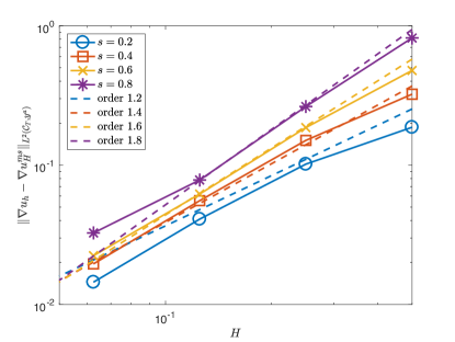
Figure 1: Convergence for the analytic example.

We take the analytic example from [42, Section 6.1] with $\Omega=(0,1)^{2}$ and so ${{\cal C}_{T}}=(0,1)^{2}\times(0,T)$ with the forcing

$$f(x_{1},x_{2})=(2\pi^{2})^{s}\sin(\pi x_{1})\sin(\pi x_{2}).$$

The exact solution on $\Omega$ is then given by $u(x_{1},x_{2})=\sin(\pi x_{1})\sin(\pi x_{2})$ and the exact solution on the extended domain $\mathcal{C}_{T}$ by

$$u(x_{1},x_{2},y)=\frac{2^{1-s}}{\Gamma(s)}(2\pi^{2})^{s/2}\sin(\pi x_{1})\sin(\pi x_{2})y^{s}K_{s}(\sqrt{2}\pi y),$$

where $K_{s}$ denotes the modified Bessel function of the second kind.

Note that $f$ is smooth in this example, hence the estimate in Theorem 5.6 can be improved to

$$\|\nabla u_{h}-\nabla u_{H}^{ms}\|_{L^{2}(\mathcal{C}_{T},y^{a})}\lesssim H^{1+s}\left\lVert f\right\rVert_{H^{1}(\Omega)}.$$

Here, Figure 1 shows the convergence of the error $\|\nabla u_{h}-\nabla u_{H}^{ms}\|_{L^{2}(\mathcal{C}_{T},y^{a})}$ for $H=2^{-1},\ldots,2^{-4}$ and $h=2^{-6}$. As predicted by the theory, we observe numerical convergence close to $\mathcal{O}(H^{1+s})$ for $s=0.2,0.4,0.6$ and $s=0.8$. Note that in this particular example we get improved convergence rates despite the fact that we used local projections ${\cal P}_{{\bf v}}^{\Omega}$. This indicates that the sum of the local projections are close to the $\Omega$-global $L^{2}$ projection in this simple example.

6.2 Heterogeneous example

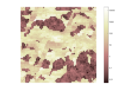
(a)

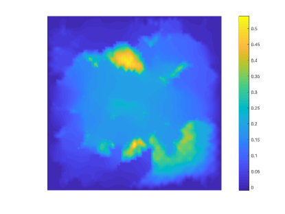
(b)

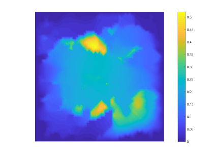
(c)

Figure 2: LABEL:sub@fig:permeability Logarithm of the chosen permeability, LABEL:sub@fig:speSolution discrete multiscale solution for $s=0.2$ and $k=2$, and LABEL:sub@fig:speFineSolution fine scale approximation for $s=0.2$ and $h=2^{-9}$ in the heterogeneous example.

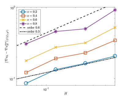
Figure 3: Convergence for the heterogeneous example.

In this example we choose again $\Omega=(0,1)^{2}$ so that ${{\cal C}_{T}}=(0,1)^{2}\times(0,T)$, and $f(x_{1},x_{2})=(2\pi^{2})^{s}\sin(\pi x_{1})\sin(\pi x_{2})$. However, we chose a non-constant diffusion coefficient that varies on the fine scale between $5\cdot 10^{-3}$ and $2\cdot 10^{4}$. The values are taken from the SPE10 benchmark problem. The logarithm of the chosen values is displayed in Figure 2a. A discrete multiscale solution for $s=0.2$ is displayed in Figure 2b, and the fine scale approximation for $s=0.2$ and $h=2^{-6}$ is displayed in Figure 2c. Comparing Figures 2b and 2c one can observe that the LOD method captures the fine scale features of the solution very well. We shall emphasize that the theory of localization (Lemma 5.3 and Appendix A) does not allow meaningful predictions on the performance of the multiscale method in the present regime of very high contrast. Still, the experimental results are promising. This has also been observed before for high-contrast local PDEs in [44, 13]. The theory therein also indicates that the success of numerical homogenization may depend on the geometric properties of the diffusion coefficient and its phases relative to the coarse mesh. In particular, a non-monotonic behavior of the error may occur depending on the relative position of coarse nodes and high and low permeability regions of the medium. In Figure 3, the convergence of the error $\|\nabla u_{h}-\nabla u_{H}^{ms}\|_{L^{2}(\mathcal{C}_{T},y^{a})}$ for $H=2^{-1},\ldots,2^{-4}$ and $h=2^{-6}$ is shown. Because of the heterogeneous coefficient, we cannot expect the local projections ${\cal P}_{{\bf v}}^{\Omega}$ to be close to the $\Omega$-global $L^{2}$ projection, hence we expect convergence rates of $\mathcal{O}(H^{s})$ from Theorem 5.4. As shown in Figure 3 we indeed observe convergence rates in the range of $\mathcal{O}(H^{s})$ despite the high contrast of the diffusion coefficient and the small truncated patches of the corrector problems. For $s=0.2$ we even see some minor improved convergence of $\mathcal{O}(H^{0.3})$ due to the boundary projections, while for $s=0.8$ the convergence of $\mathcal{O}(H^{0.6})$ is lower due to the rough truncation of the corrector problems at layer $k=2$. Note that the error of the fine-grid solution is probably much higher, so that higher computational costs for larger $k$ are not justified. The convergence for $s=0.4$ and $s=0.6$ are in between those values and therefore closer to the predicted value $\mathcal{O}(H^{s})$.

7 Conclusion

In this paper, we developed a multiscale method for heterogeneous fractional Laplacians. The method utilized a localization of multiscale correctors to obtain an efficient numerical scheme with optimal rates of convergence for the coarse-grid. We developed this method in the context of weighted Sobolev spaces to be applied to the extended domain problem of the fractional Laplacian where the coefficient of the extension has a singular/degenerate value. To this end, we constructed a quasi-interpolation that utilizes averages on $d$ and $d+1$ dimensional subsets so that the critical boundary is better resolved. We proved local stability and approximability of this operator in weighted Sobolev spaces. We then proved the error estimates and truncation arguments in this weighted setting. To confirm our theoretical results we gave two numerical experiments with various fractional orders $s$.

8 Acknowledgments

The second author has been funded by the Austrian Science Fund (FWF) through the project P 29197-N32. Main parts of this paper were written while the authors enjoyed the kind hospitality of the Hausdorff Institute for Mathematics in Bonn during the trimester program on multiscale problems in 2017.

Appendix A Truncation Proofs

Now we will prove and state the auxiliary lemmas used to prove the localized error estimate in Lemma 5.3 and Theorem 5.4. These proofs are largely based on the works [28, 37] and references therein. There are a few interesting nuances with respect to the weighted inverse and Poincaré inequalities, Muckenhoupt constant bounds, and the Caccioppoli inequality Lemma 3.9.

We begin with some notation. For ${\bf v},{\bf v}^{\prime}\in{\cal N}_{dof}$ and $l,k\in\mathbb{N}$ and $m=0,1,\cdots,$ with $k\geq l\geq 2$ we have the quasi-inclusion property:

$$\text{if}\quad{\omega}_{{\bf v}^{\prime},m+1}\cap\left({\omega}_{{\bf v},k}\backslash{\omega}_{{\bf v},l}\right)\neq\emptyset,\quad\text{then}\quad{\omega}_{{\bf v}^{\prime},1}\subset\left({\omega}_{{\bf v},k+m+1}\backslash{\omega}_{{\bf v},l-m-1}\right).$$ (47)

We will use the cutoff functions defined in [28]. For ${\bf v}\in{\cal N}_{dof}$ and $k>l\in\mathbb{N}$, let $\eta^{k,l}_{{\bf v}}:{{\cal C}_{T}}\to[0,1]$ be a continuous weakly differentiable function so that

$$\left(\eta^{k,l}_{{\bf v}}\right)|_{{\omega}_{{\bf v},k-l}} =0,$$ (48a)

$$\left(\eta^{k,l}_{{\bf v}}\right)|_{{{\cal C}_{T}}\backslash{\omega}_{{\bf v},k}} =1,$$ (48b)

$$\forall T\in{\cal T}_{{{\cal C}_{T}}},\left\lVert\nabla\eta^{k,l}_{\bf v}\right\rVert_{L^{\infty}(T)} \leq C_{co}\frac{1}{lH},$$ (48c)

where $C_{co}$ is only dependent on the shape regularity of the mesh ${\cal T}_{{{\cal C}_{T}}}$. We choose here the cutoff function as in [37], where we choose a function $\eta^{k,l}_{{\bf v}}$, in the space of $\mathbb{P}_{1}$ Lagrange finite elements over ${\cal T}_{{{\cal C}_{T}}}$, such that

$$\eta^{k,l}_{{\bf v}}({\bf v}^{\prime}) =0\text{ for all }{\bf v}^{\prime}\in{\cal N}_{dof}\cap\omega_{{\bf v},k-l},$$

$$\eta^{k,l}_{{\bf v}}({\bf v}^{\prime}) =1\text{ for all }{\bf v}^{\prime}\in{\cal N}_{dof}\cap({{\cal C}_{T}}\backslash\omega_{{\bf v},k}),$$

$$\eta^{k,l}_{{\bf v}}({\bf v}^{\prime}) =\frac{j}{l}\text{ for all }{\bf v}^{\prime}\in{\cal N}_{dof}\cap\omega_{{\bf v},k-l+j},j=0,1,\dots,l.$$

We will now prove the quasi-invariance of the fine-scale functions under multiplication by cutoff functions in weighted Sobolev spaces.

Lemma A.1.

Let $k>l\in\mathbb{N}$ and ${\bf v}\in{\cal N}_{dof}$. Suppose that $w\in{V}^{f}$, then we have the estimate

$${\left\lVert\nabla{\cal I}_{H}(\eta_{{\bf v}}^{k,l}w)\right\rVert}_{L^{2}\left({{\cal C}_{T}},y^{a}\right)}\lesssim l^{-1}{\left\lVert\nabla w\right\rVert}_{L^{2}\left({\omega}_{{\bf v},k+1}\backslash{\omega}_{{\bf v},k-l-1},y^{a}\right)}.$$

Proof.

Fix ${\bf v}$ and $k$, denote the average as ${\langle\eta_{{\bf v}}^{k,l}\rangle}_{{\omega}_{{\bf v}^{\prime},1}}=\frac{1}{|{\omega}_{{\bf v}^{\prime},1}|}\int_{{\omega}_{{\bf v}^{\prime},1}}\eta_{{\bf v}}^{k,l}\,d{\bf x}.$ For an estimate on a single patch ${\omega}_{{\bf v}^{\prime}}$, using the fact that ${\cal I}_{H}(w)=0$ and the stability (25b), we have

$${\left\lVert\nabla{\cal I}_{H}(\eta_{{\bf v}}^{k,l}w)\right\rVert}_{L^{2}\left({\omega}_{{\bf v}^{\prime}},y^{a}\right)} ={\left\lVert\nabla{\cal I}_{H}((\eta_{{\bf v}}^{k,l}-{\langle\eta_{{\bf v}}^{k,l}\rangle}_{{\omega}_{{\bf v}^{\prime},1}})w)\right\rVert}_{L^{2}\left({\omega}_{{\bf v}^{\prime}},y^{a}\right)}\lesssim{\left\lVert\nabla((\eta_{{\bf v}}^{k,l}-{\langle\eta_{{\bf v}}^{k,l}\rangle}_{{\omega}_{{\bf v}^{\prime},1}})w)\right\rVert}_{L^{2}\left({\omega}_{{\bf v}^{\prime},1},y^{a}\right)}$$

$$\lesssim\left({\left\lVert(\eta_{{\bf v}}^{k,l}-{\langle\eta_{{\bf v}}^{k,l}\rangle}_{{\omega}_{{\bf v}^{\prime},1}})\nabla w\right\rVert}_{L^{2}\left({\omega}_{{\bf v}^{\prime},1},y^{a}\right)}+{\left\lVert\nabla\eta^{k,l}_{{\bf v}}(w-{\cal I}_{H}(w))\right\rVert}_{L^{2}\left({\omega}_{{\bf v}^{\prime},1},y^{a}\right)}\right).$$

Summing over all ${\bf v}^{\prime}\in{\cal N}_{dof}$ and using the quasi-inclusion property (47) yields

$${\left\lVert\nabla{\cal I}_{H}(\eta_{{\bf v}}^{k,l}w)\right\rVert}_{L^{2}\left({{\cal C}_{T}},y^{a}\right)}^{2} \lesssim\sum_{{\omega}_{{\bf v}^{\prime}}\subset{\omega}_{{\bf v},k+1}\backslash{\omega}_{{\bf v},k-l-1}}{\left\lVert(\eta_{{\bf v}}^{k,l}-{\langle\eta_{{\bf v}}^{k,l}\rangle}_{{\omega}_{{\bf v}^{\prime},1}})\nabla w\right\rVert}_{L^{2}\left({\omega}_{{\bf v}^{\prime},1},y^{a}\right)}^{2}$$

$$+\sum_{{\omega}_{{\bf v}^{\prime}}\subset{\omega}_{{\bf v},k+1}\backslash{\omega}_{{\bf v},k-l-1}}{\left\lVert\nabla\eta^{k,l}_{{\bf v}}(w-{\cal I}_{H}(w))\right\rVert}_{L^{2}\left({\omega}_{{\bf v}^{\prime},1},y^{a}\right)}^{2}.$$ (49)

Note that we used that $\nabla\eta_{{\bf v}}^{k,l}\neq 0$ only in ${\omega}_{{\bf v},k}\backslash{\omega}_{{\bf v},k-l}$ and $(\eta_{{\bf v}}^{k,l}-{\langle\eta_{{\bf v}}^{k,l}\rangle}_{{\omega}_{{\bf v}^{\prime},1}})\neq 0$ only if ${\omega}_{{\bf v}^{\prime}}$ intersects ${\omega}_{{\bf v},k}\backslash{\omega}_{{\bf v},k-l}$, hence we obtained the slightly better bound.

We now denote $\mu_{{\bf v}}^{k,l}=\eta_{{\bf v}}^{k,l}-{\langle\eta_{{\bf v}}^{k,l}\rangle}_{{\omega}_{{\bf v}^{\prime},1}}$, and let ${T}$ be a simplex in ${{\omega}_{{\bf v}^{\prime},1}}$ such that the supremum $\left\lVert\mu_{{\bf v}}^{k,l}\right\rVert_{L^{\infty}({\omega}_{{\bf v}^{\prime},1})}$ is obtained. On ${T}$, $\mu_{{\bf v}}^{k,l}$ is an affine function, using the fact that $\eta_{{\bf v}}^{k,l}$ is taken to be $\mathbb{P}_{1}$, we have by using the inverse estimate (9) that

$$\left\lVert\mu_{{\bf v}}^{k,l}\right\rVert_{L^{\infty}({\omega}_{{\bf v}^{\prime},1})}=\left\lVert\mu_{{\bf v}}^{k,l}\right\rVert_{L^{\infty}(T)} \lesssim|T|^{-1}\left\lVert y^{-\frac{a}{2}}\right\rVert_{L^{2}(T)}\left\lVert\mu_{{\bf v}}^{k,l}\right\rVert_{L^{2}(T,y^{a})}.$$

Using the above estimate and the weighted Poincaré inequality, we see that

$$\left\lVert\eta_{{\bf v}}^{k,l}-{\langle\eta_{{\bf v}}^{k,l}\rangle}_{{\omega}_{{\bf v}^{\prime},1}}\right\rVert_{L^{\infty}({\omega}_{{\bf v}^{\prime},1})} \lesssim|{\omega}_{{\bf v}^{\prime},1}|^{-1}\left\lVert y^{-\frac{a}{2}}\right\rVert_{L^{2}({\omega}_{{\bf v}^{\prime},1})}\left\lVert\eta_{{\bf v}}^{k,l}-{\langle\eta_{{\bf v}}^{k,l}\rangle}_{{\omega}_{{\bf v}^{\prime},1}}\right\rVert_{L^{2}({\omega}_{{\bf v}^{\prime},1},y^{a})}$$

$$\lesssim|{\omega}_{{\bf v}^{\prime},1}|^{-1}\left\lVert y^{-\frac{a}{2}}\right\rVert_{L^{2}({\omega}_{{\bf v}^{\prime},1})}H\left\lVert\nabla\eta_{{\bf v}}^{k,l}\right\rVert_{L^{2}({\omega}_{{\bf v}^{\prime},1},y^{a})}$$

$$\lesssim|{\omega}_{{\bf v}^{\prime},1}|^{-1}\left\lVert y^{-\frac{a}{2}}\right\rVert_{L^{2}({\omega}_{{\bf v}^{\prime},1})}H\sum_{T\in\omega_{{\bf v}^{\prime},1}}\left\lVert\nabla\eta_{{\bf v}}^{k,l}\right\rVert_{L^{2}(T,y^{a})}$$

$$\lesssim|{\omega}_{{\bf v}^{\prime},1}|^{-1}\left\lVert y^{-\frac{a}{2}}\right\rVert_{L^{2}({\omega}_{{\bf v}^{\prime},1})}H\sum_{T\in\omega_{{\bf v}^{\prime},1}}\left\lVert y^{\frac{a}{2}}\right\rVert_{L^{2}(T)}\left\lVert\nabla\eta_{{\bf v}}^{k,l}\right\rVert_{L^{\infty}(T)}$$

$$\lesssim\left(|{\omega}_{{\bf v}^{\prime},1}|^{-1}\left\lVert y^{-\frac{a}{2}}\right\rVert_{L^{2}({\omega}_{{\bf v}^{\prime},1})}\left\lVert y^{\frac{a}{2}}\right\rVert_{L^{2}({\omega}_{{\bf v}^{\prime},1})}\right)H\left\lVert\nabla\eta_{{\bf v}}^{k,l}\right\rVert_{L^{\infty}({\omega}_{{\bf v}^{\prime},1})}$$

$$\lesssim C_{2,a}^{\frac{1}{2}}H\left\lVert\nabla\eta_{{\bf v}}^{k,l}\right\rVert_{L^{\infty}({\omega}_{{\bf v}^{\prime},1})},$$ (50)

where we used the Muckenhoupt weight bound (7), as well as quasi-uniformity of the grid. Returning to (49), using the above relation on the first term and the approximation property (26a) on the second term, we obtain

$${\left\lVert\nabla{\cal I}_{H}(\eta_{{\bf v}}^{k,l}w)\right\rVert}_{L^{2}\left({{\cal C}_{T}},y^{a}\right)}^{2} \lesssim H^{2}\left\lVert\nabla\eta_{{\bf v}}^{k,l}\right\rVert_{L^{\infty}({{\cal C}_{T}})}^{2}{\left\lVert\nabla w\right\rVert}_{L^{2}\left({\omega}_{{\bf v},k+1}\backslash{\omega}_{{\bf v},k-l-1},y^{a}\right)}^{2}$$

$$+H^{2}\left\lVert\nabla\eta_{{\bf v}}^{k,l}\right\rVert_{L^{\infty}({{\cal C}_{T}})}^{2}{\left\lVert\nabla w\right\rVert}_{L^{2}\left({\omega}_{{\bf v},k+1}\backslash{\omega}_{{\bf v},k-l-1},y^{a}\right)}^{2}.$$

Finally, we arrive at

$${\left\lVert\nabla{\cal I}_{H}(\eta_{{\bf v}}^{k,l}w)\right\rVert}_{L^{2}\left({{\cal C}_{T}},y^{a}\right)}^{2}\lesssim l^{-2}{\left\lVert\nabla w\right\rVert}_{L^{2}\left({\omega}_{{\bf v},k+1}\backslash{\omega}_{{\bf v},k-l-1},y^{a}\right)}^{2},$$

where we used $\left\lVert\nabla\eta_{{\bf v}}^{k,l}\right\rVert_{L^{\infty}({{\cal C}_{T}})}^{2}\lesssim 1/(lH)^{2}$. ∎

For the weighted Sobolev space, we have the following decay of the fine-scale space.

Lemma A.2.

Fix some ${\bf v}\in{\cal N}_{dof}$ and let $F\in({V}^{f})^{\prime}$ be the dual of ${V}^{f}$ satisfying $F(w)=0$ for all $w\in{V}^{f}({{\cal C}_{T}}\backslash{\omega}_{{\bf v},1})$. Let $u\in{V}^{f}$ be the solution of

$$\int_{{{\cal C}_{T}}}B(x)\nabla u\nabla w\,y^{a}\,d{\bf x}=F(w)\quad\text{for all }w\in{V}^{f},$$

then there exists a constant $\theta\in(0,1)$ such that for $k\in\mathbb{N}$ we have

$${\left\lVert\nabla u\right\rVert}_{L^{2}\left({{\cal C}_{T}}\backslash{\omega}_{{\bf v},k},y^{a}\right)}\lesssim\theta^{k}{\left\lVert\nabla u\right\rVert}_{L^{2}\left({{\cal C}_{T}},y^{a}\right)}.$$

Proof.

Let $\eta_{{\bf v}}^{k,l}$ be the cut-off function as in the previous lemma for $l<k-1$, $\tilde{u}=\eta_{{\bf v}}^{k,l}u-{\cal I}_{H}(\eta_{{\bf v}}^{k,l}u)\in{V}^{f}({{\cal C}_{T}}\backslash{\omega}_{{\bf v},k-l-1})$, and note that from Lemma A.1 we have

$${\left\lVert\nabla(\eta_{{\bf v}}^{k,l}u-\tilde{u})\right\rVert}_{L^{2}\left({{\cal C}_{T}},y^{a}\right)}={\left\lVert\nabla{\cal I}_{H}(\eta_{{\bf v}}^{k,l}u)\right\rVert}_{L^{2}\left({{\cal C}_{T}},y^{a}\right)}\lesssim l^{-1}{\left\lVert\nabla u\right\rVert}_{L^{2}\left({\omega}_{{\bf v},k+1}\backslash{\omega}_{{\bf v},k-l-1},y^{a}\right)}.$$ (51)

From this estimate and the properties of $F$ we have

$$\int_{{{\cal C}_{T}}\backslash{\omega}_{{\bf v},k-l-1}}B(x)\nabla u\nabla\tilde{u}\,y^{a}\,d{\bf x}=\int_{{{\cal C}_{T}}}B(x)\nabla u\nabla\tilde{u}\,y^{a}\,d{\bf x}=F(\tilde{u})=0.$$ (52)

We utilize a version of the Caccioppoli inequality from Lemma 3.9 to deduce

$${\left\lVert\nabla u\right\rVert}_{L^{2}\left({{\cal C}_{T}}\backslash{\omega}_{{\bf v},k},y^{a}\right)}^{2} \lesssim\int_{{{\cal C}_{T}}\backslash{\omega}_{{\bf v},k-l-1}}\eta_{{\bf v}}^{k,l}B(x)\nabla u\nabla u\,y^{a}\,d{\bf x}$$

$$\lesssim\int_{{{\cal C}_{T}}\backslash{\omega}_{{\bf v},k-l-1}}\nabla u\left(\nabla(\eta_{{\bf v}}^{k,l}u)-u\nabla\eta_{{\bf v}}^{k,l}\right)\,y^{a}\,d{\bf x}.$$

Using the fact that ${\cal I}_{H}(u)=0$, estimate (51), and the relation (52) we have

$${\left\lVert\nabla u\right\rVert}_{L^{2}\left({{\cal C}_{T}}\backslash{\omega}_{{\bf v},k},y^{a}\right)}^{2}\lesssim\int_{{{\cal C}_{T}}\backslash{\omega}_{{\bf v},k-l-1}}\nabla u(\nabla(\eta_{{\bf v}}^{k,l}u-\tilde{u}))\,y^{a}\,d{\bf x}-\int_{{{\cal C}_{T}}\backslash{\omega}_{{\bf v},k-l-1}}\nabla u(u-{\cal I}_{H}(u))\nabla\eta_{{\bf v}}^{k,l}\,y^{a}\,d{\bf x}$$

$$\qquad\lesssim l^{-1}{\left\lVert\nabla u\right\rVert}_{L^{2}\left({{\cal C}_{T}}\backslash{\omega}_{{\bf v},k-l-1},y^{a}\right)}^{2}+(lH)^{-1}{\left\lVert\nabla u\right\rVert}_{L^{2}\left({{\cal C}_{T}}\backslash{\omega}_{{\bf v},k-l-1},y^{a}\right)}{\left\lVert u-{\cal I}_{H}(u)\right\rVert}_{L^{2}\left({{\cal C}_{T}}\backslash{\omega}_{{\bf v},k-l-1},y^{a}\right)}$$

$$\qquad\lesssim l^{-1}{\left\lVert\nabla u\right\rVert}_{L^{2}\left({{\cal C}_{T}}\backslash{\omega}_{{\bf v},k-l-1},y^{a}\right)}^{2}.$$

On the last term we used the approximation property (26a). Successive applications of the above estimate leads to

$${\left\lVert\nabla u\right\rVert}_{L^{2}\left({{\cal C}_{T}}\backslash{\omega}_{{\bf v},k},y^{a}\right)}^{2} \lesssim l^{-1}{\left\lVert\nabla u\right\rVert}_{L^{2}\left({{\cal C}_{T}}\backslash{\omega}_{{\bf v},k-l-1},y^{a}\right)}^{2}\lesssim l^{-\lfloor\frac{k-1}{l+1}\rfloor}{\left\lVert\nabla u\right\rVert}_{L^{2}\left({{\cal C}_{T}}\backslash{\omega}_{{\bf v},1},y^{a}\right)}^{2}\lesssim l^{-\lfloor\frac{k-1}{l+1}\rfloor}{\left\lVert\nabla u\right\rVert}_{L^{2}\left({{\cal C}_{T}},y^{a}\right)}^{2}.$$

Finally, noting that

$$\left\lfloor\frac{k-1}{l+1}\right\rfloor=\left\lceil\frac{k-l-1}{l+1}\right\rceil\geq\frac{k}{l+1}-1,$$

taking $\theta=l^{-\frac{1}{l+1}}$ yields the result. ∎

We are now ready to restate our result on the error introduced from localization. This is merely Lemma 5.3 restated. When $k$ is sufficiently large so that the corrector problem is all of ${{\cal C}_{T}}$, we denote $Q_{{\bf v},k}=Q_{{\bf v},{{\cal C}_{T}}}$. Let $u_{H}\in{V}_{H}$, let $Q_{k}$ be constructed from (38), and $Q_{{{\cal C}_{T}}}$ defined to be the ideal corrector without truncation, then

$${\left\lVert\nabla(Q_{{{\cal C}_{T}}}(u_{H})-Q_{k}(u_{H}))\right\rVert}_{L^{2}\left({{\cal C}_{T}},y^{a}\right)}\lesssim k^{\frac{d}{2}}\theta^{k}{\left\lVert\nabla u_{H}\right\rVert}_{L^{2}\left({{\cal C}_{T}},y^{a}\right)}.$$ (53)

We begin the proof in a similar way as in [13].

Proof of Lemma 5.3.

We denote $v=Q_{{{\cal C}_{T}}}(u_{H})-Q_{k}(u_{H})\in{V}^{f},$ subsequently ${\cal I}_{H}(v)=0$. Taking the cut-off function $\eta_{{\bf v}}^{k,1}$ we have

$${\left\lVert\nabla v\right\rVert}_{L^{2}\left({{\cal C}_{T}},y^{a}\right)}^{2} \lesssim\sum_{{\bf v}\in{\cal N}_{dof}}\int_{{{\cal C}_{T}}}B(x)\nabla(Q_{{\bf v},{{\cal C}_{T}}}(u_{H})-Q_{{\bf v},k}(u_{H}))\nabla(v(1-\eta_{{\bf v}}^{k,1}))\,y^{a}\,d{\bf x}$$ (54)

$$+\sum_{{\bf v}\in{\cal N}_{dof}}\int_{{{\cal C}_{T}}}B(x)\nabla(Q_{{\bf v},{{\cal C}_{T}}}(u_{H})-Q_{{\bf v},k}(u_{H}))\nabla(v\eta_{{\bf v}}^{k,1})\,y^{a}\,d{\bf x}.$$ (55)

Estimating the right hand side of (54) for each ${\bf v}$, and using the boundedness of $B(x)$, we have

$$\int_{{{\cal C}_{T}}}B(x)\nabla(Q_{{\bf v},{{\cal C}_{T}}}(u_{H})-Q_{{\bf v},k}(u_{H}))\nabla(v(1-\eta_{{\bf v}}^{k,1}))\,y^{a}\,d{\bf x}$$

$$\qquad\lesssim{\left\lVert\nabla(Q_{{\bf v},{{\cal C}_{T}}}(u_{H})-Q_{{\bf v},k}(u_{H}))\right\rVert}_{L^{2}\left({{\cal C}_{T}},y^{a}\right)}{\left\lVert\nabla(v(1-\eta_{{\bf v}}^{k,1}))\right\rVert}_{L^{2}\left({\omega}_{{\bf v},k},y^{a}\right)}$$

$$\qquad\lesssim{\left\lVert\nabla(Q_{{\bf v},{{\cal C}_{T}}}(u_{H})-Q_{{\bf v},k}(u_{H}))\right\rVert}_{L^{2}\left({{\cal C}_{T}},y^{a}\right)}\left({\left\lVert\nabla v\right\rVert}_{L^{2}\left({\omega}_{{\bf v},k},y^{a}\right)}+{\left\lVert v\nabla(1-\eta_{{\bf v}}^{k,1}))\right\rVert}_{L^{2}\left({\omega}_{{\bf v},k}\backslash{\omega}_{{\bf v},k-1},y^{a}\right)}\right)$$

$$\qquad\lesssim{\left\lVert\nabla(Q_{{\bf v},{{\cal C}_{T}}}(u_{H})-Q_{{\bf v},k}(u_{H}))\right\rVert}_{L^{2}\left({{\cal C}_{T}},y^{a}\right)}\left({\left\lVert\nabla v\right\rVert}_{L^{2}\left({\omega}_{{\bf v},k},y^{a}\right)}+H^{-1}{\left\lVert v-{\cal I}_{H}(v)\right\rVert}_{L^{2}\left({\omega}_{{\bf v},k}\backslash{\omega}_{{\bf v},k-1},y^{a}\right)}\right)$$

$$\qquad\lesssim{\left\lVert\nabla(Q_{{\bf v},{{\cal C}_{T}}}(u_{H})-Q_{{\bf v},k}(u_{H}))\right\rVert}_{L^{2}\left({{\cal C}_{T}},y^{a}\right)}{\left\lVert\nabla v\right\rVert}_{L^{2}\left({\omega}_{{\bf v},k+1},y^{a}\right)}.$$

As in the proof of Lemma A.2, we denote $\tilde{v}=\eta_{{\bf v}}^{k,1}v-{\cal I}_{H}(\eta_{{\bf v}}^{k,1}v)\in{V}^{f}({{\cal C}_{T}})$ and so $\tilde{v}$ satisfies

$$\int_{{{\cal C}_{T}}}B(x)\nabla(Q_{{\bf v},{{\cal C}_{T}}}(u_{H})-Q_{{\bf v},k}(u_{H}))\nabla\tilde{v}\,y^{a}\,d{\bf x}=0.$$

We have now the estimate for (55) for ${\bf v}\in{\cal N}_{dof}$ using the above identity and (51)

$$\int_{{{\cal C}_{T}}}B(x)\nabla(Q_{{\bf v},{{\cal C}_{T}}}(u_{H})-Q_{{\bf v},k}(u_{H}))\nabla(v\eta_{{\bf v}}^{k,1}-\tilde{v})\,y^{a}\,d{\bf x}$$

$$\qquad\lesssim{\left\lVert\nabla(Q_{{\bf v},{{\cal C}_{T}}}(u_{H})-Q_{{\bf v},k}(u_{H}))\right\rVert}_{L^{2}\left({{\cal C}_{T}},y^{a}\right)}{\left\lVert\nabla(v\eta_{{\bf v}}^{k,1}-\tilde{v})\right\rVert}_{L^{2}\left({{\cal C}_{T}},y^{a}\right)}$$

$$\qquad\lesssim{\left\lVert\nabla(Q_{{\bf v},{{\cal C}_{T}}}(u_{H})-Q_{{\bf v},k}(u_{H}))\right\rVert}_{L^{2}\left({{\cal C}_{T}},y^{a}\right)}{\left\lVert\nabla v\right\rVert}_{L^{2}\left({\omega}_{{\bf v},k+1},y^{a}\right)}.$$

Combing the estimates for (54) and (55) we obtain

$${\left\lVert\nabla v\right\rVert}_{L^{2}\left({{\cal C}_{T}},y^{a}\right)}^{2} \lesssim\sum_{{\bf v}\in{\cal N}_{dof}}{\left\lVert\nabla(Q_{{\bf v},{{\cal C}_{T}}}(u_{H})-Q_{{\bf v},k}(u_{H}))\right\rVert}_{L^{2}\left({{\cal C}_{T}},y^{a}\right)}{\left\lVert\nabla v\right\rVert}_{L^{2}\left({\omega_{{\bf v},k+1}},y^{a}\right)}$$

$$\lesssim k^{\frac{d}{2}}\left(\sum_{{\bf v}\in{\cal N}_{dof}}{\left\lVert\nabla(Q_{{\bf v},{{\cal C}_{T}}}(u_{H})-Q_{{\bf v},k}(u_{H}))\right\rVert}_{L^{2}\left({{\cal C}_{T}},y^{a}\right)}^{2}\right)^{\frac{1}{2}}{\left\lVert\nabla v\right\rVert}_{L^{2}\left({{\cal C}_{T}},y^{a}\right)},$$ (56)

supposing that $\#\{{\bf v}\in{\cal N}_{dof}|{\omega}_{{\bf v}^{\prime}}\subset{\omega}_{{\bf v},k+1}\}\lesssim k^{d}$, as is guaranteed by quasi-uniformity of the coarse-grid.

For ${\bf v}\in{\cal N}_{dof}$, we estimate ${\left\lVert\nabla(Q_{{\bf v},{{\cal C}_{T}}}(u_{H})-Q_{{\bf v},k}(u_{H}))\right\rVert}_{L^{2}\left({{\cal C}_{T}},y^{a}\right)}$ and we use the Galerkin orthogonality of the local problem, that is

$${\left\lVert\nabla(Q_{{\bf v},{{\cal C}_{T}}}(u_{H})-Q_{{\bf v},k}(u_{H}))\right\rVert}_{L^{2}\left({{\cal C}_{T}},y^{a}\right)}\leq\inf_{q_{\bf v}\in{V}^{f}({\omega}_{{\bf v},k})}{\left\lVert\nabla(Q_{{\bf v},{{\cal C}_{T}}}(u_{H})-q)\right\rVert}_{L^{2}\left({{\cal C}_{T}},y^{a}\right)}.$$

Let $q_{{\bf v}}=(1-\eta^{(k-1),1}_{{\bf v}})Q_{{\bf v},{{\cal C}_{T}}}(u_{H})-{\cal I}_{H}((1-\eta^{(k-1),1}_{{\bf v}})Q_{{\bf v},{{\cal C}_{T}}}(u_{H}))\in{V}^{f}({\omega}_{{\bf v},k})$, we have

$${\left\lVert\nabla(Q_{{\bf v},{{\cal C}_{T}}}(u_{H})-Q_{{\bf v},k}(u_{H}))\right\rVert}_{L^{2}\left({{\cal C}_{T}},y^{a}\right)}^{2}$$

$$\qquad\leq{\left\lVert\nabla(\eta^{(k-1),1}_{{\bf v}}Q_{{\bf v},{{\cal C}_{T}}}(u_{H})-{\cal I}_{H}((1-\eta^{(k-1),1}_{{\bf v}})Q_{{\bf v},{{\cal C}_{T}}}(u_{H})))\right\rVert}_{L^{2}\left({{\cal C}_{T}},y^{a}\right)}^{2}$$

$$\qquad\lesssim{\left\lVert\nabla Q_{{\bf v},{{\cal C}_{T}}}(u_{H})\right\rVert}_{L^{2}\left({{\cal C}_{T}}\backslash{\omega}_{{\bf v},k-2},y^{a}\right)}^{2}+{\left\lVert\nabla({\cal I}_{H}(\eta^{(k-1),1}_{{\bf v}}Q_{{\bf v},{{\cal C}_{T}}}(u_{H})))\right\rVert}_{L^{2}\left({{\cal C}_{T}},y^{a}\right)}^{2}.$$

Using Lemma A.1 and Lemma A.2 on the second term we arrive at

$${\left\lVert\nabla(Q_{{\bf v},{{\cal C}_{T}}}(u_{H})-Q_{{\bf v},k}(u_{H}))\right\rVert}_{L^{2}\left({{\cal C}_{T}},y^{a}\right)}^{2}$$

$$\qquad\lesssim{\left\lVert\nabla Q_{{\bf v},{{\cal C}_{T}}}(u_{H})\right\rVert}_{L^{2}\left({{\cal C}_{T}}\backslash{\omega}_{{\bf v},k-2},y^{a}\right)}^{2}+{\left\lVert\nabla Q_{{\bf v},{{\cal C}_{T}}}(u_{H}))\right\rVert}_{L^{2}\left({\omega}_{{\bf v},k}\backslash{\omega}_{{\bf v},k-3},y^{a}\right)}^{2}$$

$$\qquad\lesssim{\left\lVert\nabla Q_{{\bf v},{{\cal C}_{T}}}(u_{H})\right\rVert}_{L^{2}\left({{\cal C}_{T}}\backslash{\omega}_{{\bf v},k-3},y^{a}\right)}^{2}$$

$$\qquad\lesssim\theta^{2(k-3)}{\left\lVert\nabla Q_{{\bf v},{{\cal C}_{T}}}(u_{H})\right\rVert}_{L^{2}\left({{\cal C}_{T}},y^{a}\right)}^{2}.$$

From the definition of $Q_{{\bf v},{{\cal C}_{T}}}$ from (38) with global corrector patches, we get

$${\left\lVert\nabla(Q_{{\bf v},{{\cal C}_{T}}}(u_{H})-Q_{{\bf v},k}(u_{H}))\right\rVert}_{L^{2}\left({{\cal C}_{T}},y^{a}\right)}^{2}\lesssim\theta^{2k}{\left\lVert\nabla u_{H}\right\rVert}_{L^{2}\left({\omega}_{{\bf v}},y^{a}\right)}^{2}.$$

Thus, summing over all ${\bf v}\in{\cal N}_{dof}$ and combining the above with (56) concludes the proof. ∎

References

- [1] A. Abdulle, W. E, B. Engquist, and E. Vanden-Eijnden. The heterogeneous multiscale method. Acta Numer., 21:1–87, 2012.
- [2] A. Abdulle and P. Henning. Localized orthogonal decomposition method for the wave equation with a continuum of scales. Math. Comp., 86(304):549–587, 2017.
- [3] R. A. Adams and J. J. F. Fournier. Sobolev spaces, volume 140 of Pure and Applied Mathematics. Elsevier, Amsterdam, second edition, 2003.
- [4] L. Banjai, J. M. Melenk, R. H. Nochetto, E. Otarola, A. J. Salgado, and C. Schwab. Tensor FEM for spectral fractional diffusion. ArXiv e-print, arXiv:1707.07367, 2017.
- [5] A. Bonito, J. P. Borthagaray, R. H. Nochetto, E. Otarola, and A. J. Salgado. Numerical methods for fractional diffusion. ArXiv e-print, arXiv:1707.01566, 2017.
- [6] A. Bonito and J. E. Pasciak. Numerical approximation of fractional powers of elliptic operators. Math. Comp., 84(295):2083–2110, 2015.
- [7] J. H. Bramble, J. E. Pasciak, and O. Steinbach. On the stability of the projection in . Math. Comp., 71(237):147–156, 2002.
- [8] J. H. Bramble and J. Xu. Some estimates for a weighted projection. Math. Comp., 56(194):463–476, 1991.
- [9] C. Brändle, E. Colorado, A. de Pablo, and U. Sánchez. A concave-convex elliptic problem involving the fractional Laplacian. Proc. Roy. Soc. Edinburgh Sect. A, 143(1):39–71, 2013.
- [10] S. Brenner and R. Scott. The mathematical theory of finite element methods, volume 15. Springer, 2007.
- [11] D. L. Brown and D. Gallistl. Multiscale sub-grid correction method for time-harmonic high-frequency elastodynamics with wavenumber explicit bounds. ArXiv e-print, arXiv:1608.04243, 2016.
- [12] D. L. Brown, D. Gallistl, and D. Peterseim. Multiscale petrov-galerkin method for high-frequency heterogeneous helmholtz equations. In M. Griebel and M. A. Schweitzer, editors, Meshfree Methods for Partial Differential Equations VIII, pages 85–115. Springer International Publishing, Cham, 2017.
- [13] D. L. Brown and D. Peterseim. A multiscale method for porous microstructures. Multiscale Model. Simul., 14(3):1123–1152, 2016.
- [14] X. Cabré and J. Tan. Positive solutions of nonlinear problems involving the square root of the Laplacian. Adv. Math., 224(5):2052–2093, 2010.
- [15] L. Caffarelli and L. Silvestre. An extension problem related to the fractional Laplacian. Comm. Partial Differential Equations, 32(7-9):1245–1260, 2007.
- [16] L. A. Caffarelli and P. R. Stinga. Fractional elliptic equations, Caccioppoli estimates and regularity. Ann. Inst. H. Poincaré Anal. Non Linéaire, 33(3):767–807, 2016.
- [17] A. Capella, J. Dávila, L. Dupaigne, and Y. Sire. Regularity of radial extremal solutions for some non-local semilinear equations. Comm. Partial Differential Equations, 36(8):1353–1384, 2011.
- [18] P. Clément. Approximation by finite element functions using local regularization. Rev. Française Automat. Informat. Recherche Opérationnelle Sér., 9(R-2):77–84, 1975.
- [19] C. D’Angelo. Finite element approximation of elliptic problems with Dirac measure terms in weighted spaces: applications to one- and three-dimensional coupled problems. SIAM J. Numer. Anal., 50(1):194–215, 2012.
- [20] C. D’Angelo and A. Quarteroni. On the coupling of 1D and 3D diffusion-reaction equations. Application to tissue perfusion problems. Math. Models Methods Appl. Sci., 18(8):1481–1504, 2008.
- [21] O. Defterli, M. D’Elia, Q. Du, M. Gunzburger, R. Lehoucq, and M. M. Meerschaert. Fractional diffusion on bounded domains. Fract. Calc. Appl. Anal., 18(2):342–360, 2015.
- [22] E. Di Nezza, G. Palatucci, and E. Valdinoci. Hitchhiker’s guide to the fractional Sobolev spaces. Bull. Sci. Math., 136(5):521–573, 2012.
- [23] A. Ern and J.-L. Guermond. Finite element quasi-interpolation and best approximation. ArXiv e-print, arXiv:1505.06931, 2015.
- [24] E. B. Fabes, C. E. Kenig, and R. P. Serapioni. The local regularity of solutions of degenerate elliptic equations. Comm. Partial Differential Equations, 7(1):77–116, 1982.
- [25] V. Gol’dshtein and A. Ukhlov. Weighted Sobolev spaces and embedding theorems. Trans. Amer. Math. Soc., 361(7):3829–3850, 2009.
- [26] J. Heinonen, T. Kilpeläinen, and O. Martio. Nonlinear Potential Theory of Degenerate Elliptic Equations. Dover Books on Mathematics Series. Dover Publications, 2012.
- [27] P. Henning, A. Målqvist, and D. Peterseim. A localized orthogonal decomposition method for semi-linear elliptic problems. ESAIM Math. Model. Numer. Anal., 48(5):1331–1349, 2014.
- [28] P. Henning, P. Morgenstern, and D. Peterseim. Multiscale partition of unity. In Meshfree methods for partial differential equations VII, volume 100 of Lect. Notes Comput. Sci. Eng., pages 185–204. Springer, Cham, 2015.
- [29] P. Henning and D. Peterseim. Oversampling for the multiscale finite element method. Multiscale Model. Simul., 11(4):1149–1175, 2013.
- [30] T. Y. Hou and X.-H. Wu. A multiscale finite element method for elliptic problems in composite materials and porous media. J. Comput. Phys., 134(1):169–189, 1997.
- [31] T. J. R. Hughes, G. R. Feijóo, L. Mazzei, and J.-B. Quincy. The variational multiscale method—a paradigm for computational mechanics. Comput. Methods Appl. Mech. Engrg., 166(1-2):3–24, 1998.
- [32] B. Jin, R. Lazarov, and Z. Zhou. A Petrov-Galerkin finite element method for fractional convection-diffusion equations. SIAM J. Numer. Anal., 54(1):481–503, 2016.
- [33] R. Kornhuber, D. Peterseim, and H. Yserentant. An analysis of a class of variational multiscale methods based on subspace decomposition. Math. Comp., electronic early view, 2017.
- [34] A. Kufner. Weighted Sobolev Spaces. Teubner-Texte zur Mathematik. B.G. Teubner, 1985.
- [35] J. Lions, P. Kenneth, and E. Magenes. Non-Homogeneous Boundary Value Problems and Applications. Number 1 in Grundlehren der mathematischen Wissenschaften. Springer Berlin Heidelberg, 2014.
- [36] J. L. Lions. Théorèmes de trace et d’interpolation. Annali della Scuola Normale Superiore di Pisa-Classe di Scienze, 13(4):389–403, 1959.
- [37] A. Målqvist and D. Peterseim. Localization of elliptic multiscale problems. Math. Comp., 83(290):2583–2603, 2014.
- [38] M. M. Meerschaert, J. Mortensen, and S. W. Wheatcraft. Fractional vector calculus for fractional advection–dispersion. Physica A: Statistical Mechanics and its Applications, 367:181–190, 2006.
- [39] J. Melenk and T. Apel. Interpolation and quasi-interpolation in h- and hp-version finite element spaces. In E. Stein, R. de Borst, and T. Hughes, editors, Encyclopedia of Computational Mechanics. Wiley, 2017.
- [40] B. Muckenhoupt. Weighted norm inequalities for the Hardy maximal function. Trans. Amer. Math. Soc., 165:207–226, 1972.
- [41] A. s. Nekvinda. Characterization of traces of the weighted Sobolev space on . Czechoslovak Math. J., 43(118)(4):695–711, 1993.
- [42] R. H. Nochetto, E. Otárola, and A. J. Salgado. A PDE approach to fractional diffusion in general domains: a priori error analysis. Found. Comput. Math., 15(3):733–791, 2015.
- [43] D. Peterseim. Variational multiscale stabilization and the exponential decay of fine-scale correctors. In Building bridges: connections and challenges in modern approaches to numerical partial differential equations, volume 114 of Lect. Notes Comput. Sci. Eng., pages 341–367. Springer, Cham, 2016.
- [44] D. Peterseim and R. Scheichl. Robust numerical upscaling of elliptic multiscale problems at high contrast. Comput. Methods Appl. Math., 16(4):579–603, 2016.
- [45] K. R. Rehfeldt, J. M. Boggs, and L. W. Gelhar. Field study of dispersion in a heterogeneous aquifer: 3. geostatistical analysis of hydraulic conductivity. Water Resources Research, 28(12):3309–3324, 1992.
- [46] L. R. Scott and S. Zhang. Finite element interpolation of nonsmooth functions satisfying boundary conditions. Math. Comp., 54(190):483–493, 1990.
- [47] S. A. Silling. Reformulation of elasticity theory for discontinuities and long-range forces. Journal of the Mechanics and Physics of Solids, 48(1):175–209, 2000.
- [48] P. R. Stinga and B. Volzone. Fractional semilinear Neumann problems arising from a fractional Keller-Segel model. Calc. Var. Partial Differential Equations, 54(1):1009–1042, 2015.
- [49] L. Tartar. An Introduction to Sobolev Spaces and Interpolation Spaces. Lecture Notes of the Unione Matematica Italiana. Springer Berlin Heidelberg, 2007.