Diffusiophoresis in non-adsorbing polymer solutions:
the Asakura-Oosawa model and stratification in drying films

Abstract

A colloidal particle placed in an inhomogeneous solution of smaller non-adsorbing polymers will move towards regions of lower polymer concentration, in order to reduce the free energy of the interface between the surface of the particle and the solution. This phenomenon is known as diffusiophoresis. Treating the polymer as penetrable hard spheres, as in the Asakura-Oosawa model, a simple analytic expression for the diffusiophoretic drift velocity can be obtained. In the context of drying films we show that diffusiophoresis by this mechanism can lead to stratification under easily accessible experimental conditions. By stratification we mean spontaneous formation of a layer of polymer on top of a layer of the colloid. Transposed to the case of binary colloidal mixtures, this offers an explanation for the stratification observed recently in these systems [A. Fortini et al., Phys. Rev. Lett. 116, 118301 (2016)]. Our results emphasise the importance of treating solvent dynamics explicitly in these problems, and caution against the neglect of hydrodynamic interactions or the use of implicit solvent models in which the absence of solvent backflow results in an unbalanced osmotic force which gives rise to large but unphysical effects.

I Introduction

Many coatings, from paints to cosmetics, form by the drying of a thin, initially liquid, film. The liquid film contains a dispersion of colloidal particles and other non-volatile species that are left behind after the liquid evaporates, and these form a solid film Keddie and Routh (2010); Routh (2013). Due to the importance of coatings made from drying colloidal suspensions, there is an extensive literature on this process Antonietti et al. (2000); Routh and Zimmerman (2004); Reyes and Duda (2005); Reyes et al. (2007); Luo et al. (2008); Ekanayake et al. (2009); Cardinal et al. (2010); Nikiforow et al. (2010); Trueman et al. (2012); Atmuri et al. (2012); Gorce et al. (2014); Gromer et al. (2015); Nunes et al. (2014). As the solvent (usually water) evaporates, the liquid/air interface descends at some speed $v_{\mathrm{ev}}$, pushing the non-volatile species such as colloidal particles and polymer molecules, ahead of it (Fig. 1).

Drying is a non-equilibrium process, and it creates concentration gradients. The concentration of colloid and polymer particles is high in an accumulation zone just below the descending interface, and lower near the bottom of the film. When there are concentration gradients in a mixture, there will be diffusiophoresis. Diffusiophoresis is the motion of one species in response to a gradient in the concentration of another. In this work, we focus on the motion of colloidal particles in response to a gradient in the concentration of smaller polymer molecules. We find that this diffusiophoretic motion can be strong enough to exclude the colloidal particles from a top layer of the drying film, i. e. it can drive stratification into a layer of small polymer molecules on top of a layer of the larger colloid particles.

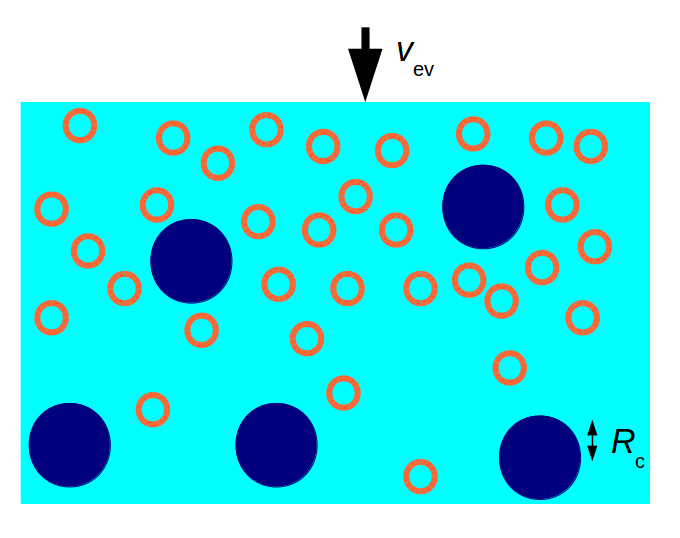
Figure 1: A schematic of a drying liquid (cyan) film containing colloidal particles (dark blue) and smaller polymer molecules (orange). The evaporation speed is $v_{\mathrm{ev}}$.

Recent experimental work Fortini et al. (2016); Martín-Fabiani et al. (2016); Makepeace et al. (2017) on making solid films via the evaporation of mixtures of colloidal particles, has found stratified dry films. Here we argue that diffusiophoresis provides a potential explanation for how this stratification occurs spontaneously during drying.

There has also been recent computer simulation and modelling work on this phenomena Fortini et al. (2016); Howard et al. (2017a); Zhou et al. (2017); Fortini and Sear (2017); Makepeace et al. (2017); Howard et al. (2017b). Indeed stratification was first discovered in simulations by Fortini et al. Fortini et al. (2016). However, to our knowledge nearly all of the existing work used an implicit solvent, i. e. modelled or simulated the particles as diffusing in a uniform continuum of some viscosity $\eta$, neglecting hydrodynamic interactions (a notable exception is Cheng and Grest Cheng and Grest (2013) who use molecular dynamics with an explicit solvent). In models with an implicit solvent that is set to be uniform, only gradients in the chemical potentials of the colloidal particles, and hence in the osmotic pressure, are possible. It is the gradient in the chemical potential of the small colloidal species, or equivalently in the osmotic pressure, that drives stratification in these models Fortini et al. (2016); Howard et al. (2017a); Zhou et al. (2017). Here we consider the solvent explicitly and find that in an evaporating film the solvent backflow leads to a counter-gradient in the solvent pressure, that we expect to balance the gradient in the osmotic pressure. Neglecting backflow, as has been done for simplicity in much of the current work, therefore appears to be an unjustified approximation.

The current resurgence of interest in diffusiophoresis has largely focused on particles driven by electrolyte gradients, where there are significant effects additionally arising from diffuse liquid junction potentials Prieve et al. (1984); Ebel et al. (1988); Staffeld and Quinn (1989a); Abécassis et al. (2008); Prieve (2008); Palacci et al. (2012); Reinmüller et al. (2013); Florea et al. (2014); Kar et al. (2015); Paustian et al. (2015); Banerjee et al. (2016); Musa et al. (2016); Shin et al. (2016). However, diffusiophoresis also occurs in gradients of uncharged solutes Anderson et al. (1982); Staffeld and Quinn (1989b); Anderson (1989); Velegol et al. (2016); Marbach et al. (2017); Yoshida et al. (2017), and we will apply expressions from this literature to polymer solutions. Our model for a polymer is the Asakura-Oosawa (AO) model Asakura and Oosawa (1954); Vrij (1976); Binder et al. (2014), where the polymer itself is ideal (no polymer-polymer interactions) but is excluded from a layer of solvent of thickness $R$ around each colloidal particle. The radius $R$ is comparable to the radius of gyration of the polymer. This is a very simple model, and we believe that this paper can also serve as a pedagogical introduction to diffusiophoresis, identifying the molecular origins of the phenomena and highlighting the importance of solvent backflow Derjaguin et al. (1947); Ruckenstein (1981); Anderson (1986, 1989); Marbach et al. (2017).

The remainder of this paper is divided into four sections. In the first section we obtain an expression for the diffusiophoretic drift velocity of a large colloidal particle in a solution of much smaller AO-model polymers. Then we compare our approach in which solvent flow is taken into account, with earlier work with an implicit solvent, where solvent flow was neglected. We then study diffusiophoresis in a drying film containing colloidal particles and smaller polymer molecules. Our final section is a conclusion.

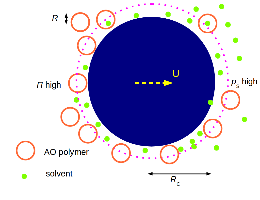
Figure 2: A schematic of a large particle (blue) immersed in a solution of AO-model polymer (orange) of radius $R$, in a solvent of smaller molecules (green). The particle excludes the polymer from layer of width $R$ (indicated by a dotted line). Along the horizontal direction, there are gradients of both the polymer contribution to the pressure ($\Pi$), and the solvent contribution ($p_{\mathrm{s}}$).

II Diffusiophoresis in the Asakura-Oosawa model

We are interested in determining the diffusiophoretic drift velocity $U$ of a colloidal particle in a solution of much smaller polymer. There is a gradient $\nabla\rho_{p}$ in the concentration of the polymer. This is illustrated in Fig. 2.

II.1 Slip velocity at flat hard wall

As we are in the $R_{c}\gg R$ limit, the curvature of the surface of the colloid can be neglected, and we can thus start by considering the relative, or slip, velocity $v_{s}$ between a hard wall (surface of large colloid) and the polymer solution. To calculate this we consider the geometry shown in Fig. 3, where the wall and gradient are along the $x$ axis. For diffusiophoresis of a solid particle, the stresses and hence the velocity gradients are localised to the interfacial region Anderson (1989). Here this is a region of width $R$. The standard theory of diffusiophoresis Anderson et al. (1982); Anderson (1989) yields the following expression for the wall slip velocity

$$v_{s}=-\frac{k_{\mathrm{B}}T}{\eta}\Bigl{[}\int_{0}^{\infty}\!\!z\,(e^{-\beta\varphi(z)}-1)\,dz\Bigr{]}\,\nabla_{x}\rho_{p}\,,$$ (1)

where $\eta$ is the viscosity (assumed equal to the bulk viscosity), $\varphi(z)$ is the potential between the solute molecules and the wall, and $\beta=1/k_{\mathrm{B}}T$. This result applies to an ideal solute whose concentration gradient in the fluid is $\nabla_{x}\rho_{p}$, and was first identified by Derjaguin and co-workers in 1947 Derjaguin et al. (1947).

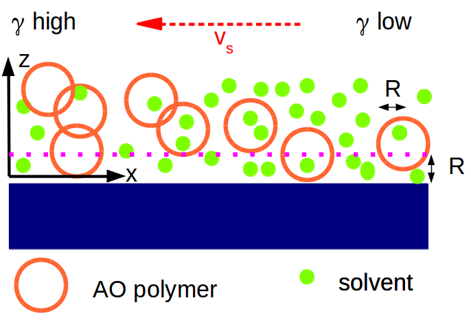
Figure 3: A schematic of a flat wall (blue) in contact with AO-model polymer (orange) in a solvent of smaller molecules (green). The wall excludes the polymer from layer of width $R$, the top of this layer is indicated by a dotted line. There are gradients of both the polymer and solvent concentrations, parallel to the wall along the $x$ axis. The flat wall is assumed stationary, and then the fluid flows to the left. $\gamma$ is the wall/solution surface free energy.

For the AO model, the wall potential is just

$$\varphi(z)=\left\{\begin{array}[]{ll}\infty&z<R\,,\\[3.0pt] 0&z>R\,.\end{array}\right.$$ (2)

With this potential, the integral in square brackets in Eq. (1) is just minus the first moment of the width of the exclusion region, i. e. $\frac{1}{2}R^{2}$. Then the slip velocity

$$v_{s}=\frac{R^{2}k_{\mathrm{B}}T}{2\eta}\,\nabla_{x}\rho_{p}$$ (3)

(this basic result can be found in Anderson’s review Anderson (1989)). Note that the slip velocity results in flow away from low concentrations of the polymer and towards higher concentrations. This can be understood as a wall-bounded Maragoni-like flow away from where the surface tension is low, and towards where it is high Ruckenstein (1981). This motion reduces the total wall/solution surface free energy, as the region of low AO-model polymer concentration expands. We show in Appendix A, that the AO-model polymer contributes $\rho_{p}k_{\mathrm{B}}TR$ to the surface tension, and so the surface tension is highest where the concentration of AO-model polymer is highest, driving flow of the solution to these high polymer concentration regions.

Eq. (1) rests on the fact that in a mixture relaxing by diffusion, the hydrostatic pressure $p$ is uniform, so that a gradient in the osmotic pressure $\Pi$ is balanced by a countergradient in the solvent contribution to the pressure. The hydrostatic pressure is uniform because it is a ‘fast’ variable which relaxes via solvent flow, and so gradients in $p$ are quickly eliminated. (We also assume other gradients, for example, in the temperature are negligible.) But the osmotic pressure (and hence counterbalancing solvent contribution to the pressure) only relax via diffusive motion of the polymer, which is much slower. This consideration will be crucial in considering implicit versus explicit solvent models. Details of the gradients in the interfacial region are in Appendix B.

II.2 Diffusiophoretic drift of large colloidal particle

For a particle of size $R_{c}\gg R$, curvature of the interface is negligible. Then, the diffusiophoretic drift velocity of such a particle in a stationary fluid is $U=-v_{s}$, where $v_{s}$ is the above slip velocity at particle’s surface. This apparently trivial result hides a great deal of subtlety in terms of the underlying low Reynolds number flow problem Levich (1962); Anderson et al. (1982); Anderson (1989). Thus one has

$$U=\Gamma\,\nabla\ln\phi_{\mathrm{p}}\,,\quad\Gamma=-\frac{\phi_{\mathrm{p}}k_{\mathrm{B}}T}{2\eta R}\sim-\phi_{\mathrm{p}}D_{p}\,.$$ (4)

where we have introduced a diffusiophoretic drift coefficient $\Gamma$. We also define $\phi_{\mathrm{p}}\equiv\rho_{p}R^{3}$ as the dimensionless polymer concentration (i. e. packing fraction). The final order-of-magnitude scaling estimate rests on the Stokes-Einstein expression for the diffusion coefficient of the polymer, $D_{p}\sim k_{\mathrm{B}}T/(\eta R)$.

The drift is away from the high polymer concentration regions, i. e. it tends to cause the large colloid to segregate from the smaller polymer. This can be understood as being driven by the reduction in surface free energy when the colloid moves to regions of lower polymer concentration where the surface tension between the colloid particle and the polymer solution is lower.

Colloidal particles can also move under the action of gravity (i. e. in sedimentation). But it is important to note that diffusiophoretic motion and sedimentation are fundamentally different Anderson (1986); Brady (2011). In sedimentation there is an external force (gravity) acting on the particle and this causes the falling particle to set up a long-ranged $1/r$ flow field in the surrounding liquid. By contrast in diffusiophoresis, the stresses and velocity gradients are largely localised to the interfacial region (here of thickness $R$), and the flow outside the immediate interface is much weaker and decays as $1/r^{3}$ Anderson (1986, 1989) .

II.3 Typical diffusiophoretic drift velocities

We now estimate how fast are typical diffusiophoretic drift velocities. For water at room temperature, $k_{\mathrm{B}}T\approx 4\times 10^{-21}\,\mathrm{J}$, and $\eta\approx 10^{-3}\,\mathrm{Pa\,s}$. We consider a polymer of radius $R\approx 10\,\mathrm{nm}$, with a maximum concentration $\phi_{\mathrm{p}}\approx 1$. Then the diffusiophoretic drift coefficient $\Gamma\approx-200\,\upmu\mathrm{m}^{2}\,\mathrm{s}^{-1}$. Thus if the length scale of the gradient $\lambda_{G}=100\,\upmu\mathrm{m}$, then the drift velocity $U$ is of order $1\,\upmu\mathrm{m}$ per second, and independent of the size of the large particle .

As noted in recent experimental work Abécassis et al. (2008); Kar et al. (2015); Shin et al. (2016), diffusiophoresis can be considerably more effective than diffusion at transporting micron-sized colloid particles over large distances. Rates of transport by directed motion (diffusiophoresis, flow, etc) can be compared to rates by diffusion via Péclet numbers. Here the Péclet number comparing diffusion to diffusiophoretic motion for the colloidal particle is

$${\cal P}_{\mathrm{coll}}=\frac{U\lambda_{G}}{D_{c}}\sim\frac{\phi_{\mathrm{p}}D_{p}}{D_{c}}$$ (5)

where $D_{c}$ is the diffusion coefficient of the colloid. We used the scaling result for $\Gamma$ in Eq. (4) to obtain the final expression, invoking $U=\Gamma\,\nabla\ln\phi_{\mathrm{p}}$ and $\nabla\ln\phi_{\mathrm{p}}\sim 1/\lambda_{G}$. Because of this the Péclet number is independent of the length scale of the gradient in the polymer concentration. For large colloidal particles $D_{c}\ll D_{p}$ and if $\phi_{\mathrm{p}}$ is not too small, diffusiophoretic motion will always be faster over all length scales (larger than $R_{c}$) on which there is a gradient.

III Earlier work on drying films, where an implicit solvent was used

In earlier work that one of us (RPS) was involved in, an osmotic imbalance mechanism was proposed to explain the motion of large colloidal particles in a concentration gradient of smaller colloidal particles Fortini et al. (2016); Fortini and Sear (2017). This model was used as a possible explanation for the stratification seen in the drying film experiments Fortini et al. (2016); Martín-Fabiani et al. (2016); Makepeace et al. (2017). Zhou et al. Zhou et al. (2017) proposed what is in effect a simple dynamic density functional theory (DDFT), while Howard et al. Howard et al. (2017a, b) proposed a more advanced DDFT; see Appendix D for a discussion of DDFT. In all these models, there is no explicit solvent. The Langevin dynamics simulations Fortini et al. (2016); Fortini and Sear (2017); Howard et al. (2017a, b) also use an implicit solvent. There the solvent is replaced by friction against a stationary background, plus a corresponding noise term. The models Fortini et al. (2016); Fortini and Sear (2017); Zhou et al. (2017); Howard et al. (2017a, b) all use the Stokes expression ($6\pi R_{c}\eta v$, at velocity $v$) for the drag in a stationary fluid. In the experiments there is, of course, a solvent (water).

The osmotic imbalance mechanism Fortini et al. (2016); Fortini and Sear (2017) argues that the gradient in the concentration of the smaller colloidal species gives rise to an imbalance in the osmotic pressure across the diameter of the large particles, leading to a drift velocity of the larger colloid. (The same argument would apply for a colloid particle in a polymer solution.) The work of Zhou et al. Zhou et al. (2017) and of Howard et al. Howard et al. (2017a, b) is similar in the sense that they too have models for stratification, in which there is an implicit solvent. Earlier work Routh (2013) on colloids in evaporating films has also used an implicit solvent.

In Ref. Fortini et al., 2016 the size of the effect was estimated as follows. The osmotic pressure difference across the particle diameter is of the order $R_{c}\,\nabla(\rho_{p}k_{\mathrm{B}}T)$. This gives rise to a force

$$F\sim-R_{c}^{3}\,\nabla(\rho_{p}k_{\mathrm{B}}T)$$ (6)

since the area over which the osmotic pressure difference acts is of order $R_{c}^{2}$. We see that this is essentially equal to the volume of the large particle multiplied by the osmotic pressure gradient, as in the generalised Archimedes principle which applies in sedimentation equilibrium Piazza et al. (2012). Ref. Fortini et al., 2016 then argued that the force $F$ leads to a drift velocity $U$ in accordance with the Stokes mobility, $U=F/(6\pi\eta R_{c})$. Using Eq. (6) this predicts a velocity

$$U\sim-\Bigl{(}\frac{R_{c}}{R}\Bigr{)}^{2}\times\frac{\phi_{\mathrm{p}}k_{\mathrm{B}}T}{\eta R}\times\nabla\ln\rho_{p}\qquad\text{[incorrect]}$$ (7)

where we emphasise that we now regard this result as containing an incorrect scaling with particle size. Compared to the correct diffusiophoretic drift velocity in Eq. (4), the result above is a factor $(R_{c}/R)^{2}$ larger, and would overwhelm the former for $R_{c}/R\gg 1$.

However, both this equation and the Langevin dynamics simulations neglect the solvent dynamics. We now discuss why this is incorrect, and in particular why solvent backflow critically modifies the above result. This observation is not new, and indeed Jülicher and Prost make the same point in a different context Jülicher and Prost (2009). The complete story can be found in a tour-de-force analysis by Brady Brady (2011). Our exposition takes a different, more informal approach, but we believe the essential point is the same.

The key point is that the force acting on the particle should additionally include a contribution from the solvent pressure gradient, as well as the osmotic pressure gradient from the solute. The solvent pressure gradient arises from solvent backflow, which must always be present in a counter-diffusing solute-plus-solvent mixture (i. e. relaxing by collective or mutual diffusion). Then, it is relatively simple to demonstrate that the solvent force apparently perfectly cancels the osmotic imbalance force.

We first recall the fundamental definition of the osmotic pressure $\Pi$, as the difference between the actual (hydrostatic) pressure $p$ in the system of interest, and the pressure $p_{s}(\mu_{s})$ in a system comprising pure solvent at the same chemical potential Guggenheim (1949); Atkins and de Paula (2014), viz.

$$p=\Pi+p_{s}(\mu_{s})\,.$$ (8)

When there is a gradient in the concentration of a colloidal or polymer species there will be a gradient in the osmotic pressure $\Pi$. However, in the absence of an external body force (like gravity, in a sedimentation equilibrium), the hydrostatic pressure rapidly relaxes by bulk flow to become uniform ($\nabla p=0$), on a time scale which is much faster than colloidal particles or polymers can diffuse to eliminate a gradient in the osmotic pressure. If $p$ is uniform, we have that the osmotic pressure and the solvent pressure have equal and opposite gradients ($\nabla\Pi=-\nabla p_{s}$). Applying the above osmotic imbalance argument we conclude that the force arising from the solvent pressure gradient cancels that arising from the osmotic pressure gradient, or in other words the net force $R_{c}^{3}\,\nabla p=0$ (since $\nabla p=0$).

At this point we have apparently argued ourselves into a corner: if there is no net force, there can be no drift, and no stratification mechanism. However such a conclusion is incorrect, as the theory of diffusiophoresis shows. Whilst there is indeed no net force, there is a force dipole at the wall, arising from the solute structuring by the wall potential. In the present case (AO model) this can be turned into a quantitative argument which recovers the classical diffusiophoretic drift velocity, highlighting that it is in fact the gradient in the solvent pressure, in the exclusion layer adjacent to the particle, that causes the drift in the AO model case. This is explained in Appendix B.

To complete the story we return briefly to sedimentation equilibrium. In this case, it is the solvent pressure $p_{s}(\mu_{s})$ that must be constant, not the hydrostatic pressure $p$. The former is constant because in equilibrium the solvent chemical potential $\mu_{s}$ is everywhere the same; the latter (hydrostatic pressure) is not constant because there is a body force acting on the fluid as a whole, due to gravity. Invoking Eq. (8) once more, we see that $\nabla p=\nabla\Pi$ in this case, and thus the integrated effect of the hydrostatic pressure gradient can be accounted to an osmotic pressure gradient, which leads to a force on the particle. Balancing this force against gravity recovers the generalised Archimedes principle Piazza et al. (2012). Thus in sedimentation equilibrium it is possible to ignore the solvent degrees of freedom.

In implicit solvent models, such as the Langevin dynamics simulations and the DDFT models used to describe film drying Howard et al. (2017a, b); Zhou et al. (2017), solvent backflow is ignored. Zhou et al.’s Zhou et al. (2017) model is effectively a simple DDFT. The result is of course that the effect of $\nabla p_{s}$ is thrown out, leaving the osmotic pressure imbalance force $R_{c}^{3}\,\nabla\Pi$. Put another way, if we simplify a model by using an implicit solvent that is defined to be uniform (and indeed static), then unbalanced gradients in the osmotic pressure appear as though they arise from an external force such as gravity. As we have just argued, this mistake leads to a grossly overestimated drift velocity, with the ‘wrong’ size scaling, as in Eq. (7). Therefore, implicit-solvent models should be used with caution when applied to dynamical situations, including interpreting experimental data on drying films.

Although the above story is complete, there is an alternative viewpoint that is worth touching upon. As Brady has emphasised Brady (2011), another way to think about the problem is to retain an explicit representation of the solute particles (polymers, in the AO model), and incorporate the correct physics by properly accounting for hydrodynamic interactions. From this viewpoint, there is indeed an imbalanced osmotic pressure gradient force on a colloid particle, and this indeed leads to a ‘primary’ drift velocity in accord with the Stokes mobility. However, this primary effect is almost completely cancelled by the long-range hydrodynamic interactions, which account for the solvent backflow.

Returning momentarily to the DDFT modeling, we show in Appendix D that this formalism gives rise to chemical potential gradients which can essentially be ascribed to unbalanced osmotic pressure gradients. Since the underlying density functional theories are known to be very accurate Schmidt et al. (2000); Roth (2010), it would be nice to find a way to incorporate this into the modeling. The ‘missing link’ appears to be in the specification of the Onsager coefficients which relate the chemical potential gradients to the fluxes (see Appendix D). In the recent work Zhou et al. (2017); Howard et al. (2017a, b) the Onsager coefficients were chosen to correspond to independent Stokes mobilities (i. e. friction against a stationary background), neglecting hydrodynamic interactions as an obvious simplification. With hindsight, it is clear that much more careful attention needs to be paid to this aspect. We leave this for future work.

IV Application of Asakura-Oosawa model to film drying

We now turn to the application of the theory in Section II to the problem of stratification of colloid particles in a drying polymer solution, first considering the sub-problem of the distribution of the polymer.

IV.1 Distribution of Asakura-Oosawa model polymer in a drying film

The presence or absence of gradients in the concentration of the polymer, is determined by a competition between the evaporation speed $v_{\mathrm{ev}}$, and diffusion of the polymer. This is quantified by the Péclet number Trueman et al. (2012); Routh (2013); Fortini et al. (2016); Fortini and Sear (2017) for the AO-model polymer molecules in the drying film, ${\cal P}_{\mathrm{film}}$, which compares the time scale for diffusion to that for drying of the film. This is defined by

$${\cal P}_{\mathrm{film}}=\frac{v_{\mathrm{ev}}H}{D_{p}}$$ (9)

where $H$ is the film thickness. If ${\cal P}_{\mathrm{film}}<1$ drying is slower than diffusion. Diffusion smooths out concentration gradients, and so here there are only weak gradients. But if ${\cal P}_{\mathrm{film}}\gtrsim O(1)$, diffusion cannot keep up with accumulation below the descending interface. Hence gradients will form and diffusiophoresis will occur.

The analysis is facilitated by a happy coincidence: since the polymer molecules in the AO model are by definition ideal, we can use the exact solution for a diffusing ideal gas in front of a moving impermeable wall to represent the effect of the drying solvent front. This leads us to consider a diffusing ideal gas between two impenetrable walls. A diffusing ideal gas satisfies

$$\frac{\partial\phi_{\mathrm{p}}}{\partial t}=D_{p}\frac{\partial^{2}\phi_{\mathrm{p}}}{\partial z^{2}}$$ (10)

with the $z$ axis normal to the walls. The boundary conditions are the two walls, plus the initial condition that at time $t=0$, we have a uniform distribution of the polymer, at an initial packing fraction $\phi_{0}$.

The bottom wall is fixed at $z=0$. This models the substrate the film is on. The boundary condition here is just zero flux. The top wall is the solvent/air interface and is descending at speed $v_{\mathrm{ev}}$. It therefore has a position

$$z_{\mathrm{int}}(t)=H-v_{\mathrm{ev}}t=(1-t^{*})H$$ (11)

at time $t$, where we have defined the reduced time

$$t^{*}=\frac{v_{\mathrm{ev}}t}{H}\quad({}\leq 1)\,.$$ (12)

Here the boundary condition is

$$D_{p}\left(\frac{1}{\phi_{\mathrm{p}}}\frac{\partial\phi_{\mathrm{p}}}{\partial z}\right)_{z_{\mathrm{int}},t}=-v_{\mathrm{ev}}$$ (13)

which is just the criterion for a diffusing ideal gas that the particles actually at the descending interface must be descending at the same speed as the interface.

In general we must solve for $\phi(z,t)$ numerically. However in the limit we are mostly interested in, where ${\cal P}_{\mathrm{film}}\gg 1$, there is range of times $t^{*}$ where a gradient is established but where the gradient is far from the bottom surface, i. e. where the accumulation zone beneath the descending interface has not yet reached the bottom. Then the profile can be obtained by taking the $H\to\infty$ limit and using the exact solution in that limit of Fedorchenko and Chernov Fedorchenko and Chernov (2003), see Appendix C.

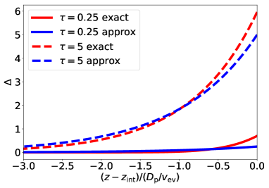
Figure 4: Plots of excess AO-model polymer $\Delta(z,\tau)$ accumulating in front of a wall moving at speed $v_{\mathrm{ev}}$ (see Appendix B). The red curves are the exact solution of Fedorchenko and Chernov Fedorchenko and Chernov (2003), while the blue curves are the approximate solution in Eq. (14). The solid curves are at the early time $\tau=tv_{\mathrm{ev}}^{2}/D_{p}=0.25$ when the gradient is being established, while the dashed curves are at the later time $\tau=5$, when the exponential $z$ dependence is well established. At still later times, the height of the exponential continues to increase linearly, while the width remains constant.

The full solution of Fedorchenko and Chernov Fedorchenko and Chernov (2003); Poon and Peters (2013) is a little complicated, but after short time $t^{*}=1/{\cal P}_{\mathrm{film}}$, an accummulation zone is established of constant width $D/v_{\mathrm{ev}}$, and linearly increasing height. In that regime ($t^{*}{\cal P}_{\mathrm{film}}\gg 1$), the solution simplifies to

$$\phi_{\mathrm{p}}(z,t)\approx\phi_{0}\left(1+{\cal P}_{\mathrm{film}}t^{*}\exp\left[-\frac{|z-z_{\mathrm{int}}|}{D_{p}/v_{\mathrm{ev}}}\right]\right)\,.$$ (14)

We have plotted profiles in Fig. 4.

The gradient in $\phi_{\mathrm{p}}$ in this regime ($t^{*}{\cal P}_{\mathrm{film}}\gg 1$) is

$$\frac{\partial\phi_{\mathrm{p}}(z,t)}{\partial z}\approx\frac{v_{\mathrm{ev}}\phi_{0}{\cal P}_{\mathrm{film}}t^{*}}{D_{p}}\exp\left[-\frac{|z-z_{\mathrm{int}}|}{D_{p}/v_{\mathrm{ev}}}\right]\,.$$ (15)

Both $\phi_{\mathrm{p}}$ and its gradient are a maximum at the interface.

IV.2 Diffusiophoresis in a drying film

We now want to calculate the effect of diffusiophoresis on colloidal particles in a drying film. To do this we simply combine the results for diffusiophoresis in AO-model polymer gradient, Eq. (4), with Eq. (15) for the gradient in a drying film. This gives the diffusiophoretic drift velocity

$$U(z,t)=-v_{\mathrm{ev}}{\cal P}_{\mathrm{film}}\phi_{0}t^{*}\exp\left[-\frac{|z-z_{\mathrm{int}}|}{D_{p}/v_{\mathrm{ev}}}\right]\,.$$ (16)

The dynamics of the colloidal particles during drying of the film are determined by the competition between two velocities: $U$ and $v_{\mathrm{ev}}$. To begin with we keep things as simple as possible and neglect diffusion (the $D_{c}\to 0$ limit). In this limit a particle below the interface moves down with speed $U(z,t)$, while actually at the interface the descending interface velocity $-v_{\mathrm{ev}}$ forms an upper bound to the particle velocity. In other words, at the interface particles must descend at least as fast as the interface, but can go faster. Thus in a drying film the velocity of a colloidal particle is

$$v_{c}(z,t)\sim\left\{\begin{array}[]{ll}\min\left(-v_{\mathrm{ev}},-v_{\mathrm{ev}}{\cal P}_{\mathrm{film}}\phi_{0}t^{*}\right)\,,&(z=z_{\mathrm{int}})\\[3.0pt] U(z,t)\,.&(z<z_{\mathrm{int}})\end{array}\right.$$ (17)

If we look at the behaviour actually at the interface, we have

$$v_{c}(z_{\mathrm{int}},t)\sim\left\{\begin{array}[]{ll}-v_{\mathrm{ev}}\,,&({\cal P}_{\mathrm{film}}\phi_{0}t^{*}\leq 1)\\[3.0pt] -v_{\mathrm{ev}}{\cal P}_{\mathrm{film}}\phi_{0}t^{*}\,.&({\cal P}_{\mathrm{film}}\phi_{0}t^{*}>1)\end{array}\right.$$ (18)

There are thus two regimes, the first is for $|U|<v_{\mathrm{ev}}$, where the particles are swept up by the descending interface, forming a layer there. The second is for $|U|>v_{\mathrm{ev}}$, where diffusiophoretic motion is faster than the speed of descent of the interface. Then the colloidal particles outrun the descending interface, and no particles accumulate at the interface. In this latter case the colloidal particles are depleted from a layer of thickness of order $D_{p}/v_{\mathrm{ev}}$ below the interface, this is the thickness of the accumulated layer of polymer.

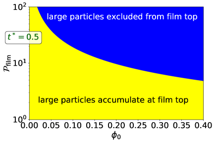
Figure 5: Plot of the $({\cal P}_{\mathrm{film}},\phi_{0})$-plane, separated into the region where the large particles accumulate at the descending interface at the top of the drying film (yellow), and the region where the large particles are excluded from the region at the top of drying film just below the interface (blue). Large values of ${\cal P}_{\mathrm{film}}$ and $\phi_{0}$ give rise to strong diffusiophoresis and drive particles away from the top of the film.

IV.3 When ${\cal P}_{\mathrm{film}}$ and $\phi_{0}$ are large, stratification occurs with depletion of colloidal particles from a top layer

As the reduced time $t^{*}\leq 1$, then unless the product ${\cal P}_{\mathrm{film}}\phi_{0}>1$ depletion of the particles from the top surface will not occur during drying. In Fig. 5 we show the $({\cal P}_{\mathrm{film}},\phi_{0})$-plane, and have shaded in blue the region where depletion has started by the time $t^{*}$ reaches $1/2$. This figure follows a similar plot made by Zhou et al. Zhou et al. (2017) for their model. The curve separating the regions of accumulation and depletion is

$${\cal P}_{\mathrm{film}}=1/\left(\phi_{0}t^{*}\right)\quad\Bigl{(}{}=2/\phi_{0}\>\>\text{for}\>\>t^{*}=1/2\Bigr{)}\,.$$ (19)

Note that there is always accumulation of the colloidal particles at early times as then there are no gradients. Gradients take time to build up. But at high enough polymer concentrations and Péclet numbers, this turns to depletion of the colloidal particles from the top layer, later on during drying.

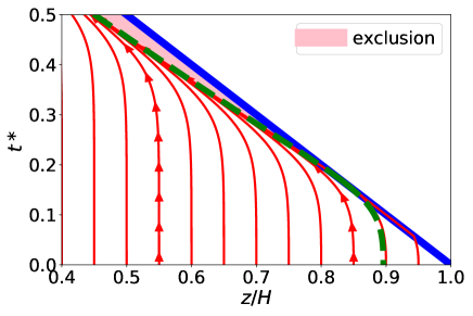
Figure 6: Trajectories $z(t^{*})$ of a large particle as a function of reduced time $t^{*}$ (red curves). Two of the trajectories have arrows to indicate the direction of the movement. The position of the top interface, $z_{\mathrm{int}}$, is shown in blue. The green dashed curve is the separatrix that divides trajectories that touch the top interface from those that do not. Colloidal particles are excluded from the triangular region between the green dashed curve and the interface. This exclusion zone is shaded in pink. Calculations are for ${\cal P}_{\mathrm{film}}=20$ and $\phi_{0}=0.3$.

In the absence of diffusion, the velocity $v_{c}(z,t)$ in Eq. (17) completely describes the time evolution of the positions of the particles during drying. The height of a particle at time $t$ is simply obtained by integrating ${\rm d}z(t)/{\rm d}t=v_{\rm C}$. Using this we further develop our understanding of the behaviour of the large particles in a drying film by considering the fate of a set of particles that at $t=0$, are uniformly spaced across the height of the film. The results are shown as the red curves in Fig. 6, where each red curve followed upwards traces out the trajectory of a particle. The blue line is the position of the top interface. Trajectories that start near the bottom of the film (i. e. left hand side of plot) are relatively unaffected and remain close to vertical, those in the middle of the film are pushed to the left away from the interface, while those near the top hit the descending interface for a time, and then later are pushed away from the top (assuming they can escape the interface).

Note that particles that start near the top of the initial wet film are caught by the descending interface early on in drying. But then later as the polymer gradient increases, these particles are pushed away from the descending interface. For the parameters used in Fig. 6, $U$ at the surface exceeds $v_{\mathrm{ev}}$ at $t^{*}\approx 0.17$ (being the point where the green dashed separatrix touches the interface). At later times there is an expanding zone beneath the descending interface where $|U|>v_{\mathrm{ev}}$ and so the colloidal particles are pushed down to further away from the interface. This exclusion region is shown in pink in Fig. 6 and there are no colloidal particles in it, but the concentration of the AO-model polymer is highest there. In this sense the AO-model polymer and the particles have kinetically segregated in the drying film, with the smaller AO-model polymer on top. This is as found in earlier work on mixtures of small and large colloidal particles Fortini et al. (2016); Fortini and Sear (2017); Martín-Fabiani et al. (2016); Howard et al. (2017a); Zhou et al. (2017); Makepeace et al. (2017).

Unlike in earlier modelling work we have taken solvent flow into account. However, our model polymer is simple, and we have not considered colloid-colloid interactions, so our predictions may not apply for high colloid packing fractions. The width of the layer without colloidal particles is set by the width of the accumulation zone of the AO-model polymer, which is $D_{p}/v_{\mathrm{ev}}$. For polymer of radius $R=10\,\mathrm{nm}$ in water, $D_{p}\approx 20\,\upmu\mathrm{m}^{2}\,\mathrm{s}^{-1}$ and so at an evaporation rate of $v_{\mathrm{ev}}=0.1\,\upmu\mathrm{m}\,\mathrm{s}^{-1}$ Utgenannt et al. (2016); Ekanayake et al. (2009), this gives a top layer $200\,\upmu\mathrm{m}$ thick. This evaporation rate is typical for room temperature evaporation of water in still air, heating Utgenannt et al. (2016) can increase this by a factor of 10, which decreases the top layer thickness to $20\,\upmu\mathrm{m}$.

It is worth noting that as typical film thicknesses are hundreds of microns Keddie and Routh (2010); Ekanayake et al. (2009), and evaporation rates range from 0.1–$1\,\upmu\mathrm{m}\,\mathrm{s}^{-1}$, that for polymers (or particles) $10\,\mathrm{nm}$ across, film Péclet numbers will be in the range 1–100. Film Péclet numbers for larger colloidal particles will then be in the range 10–$10^{4}$. However, for small molecules (e. g. ions, co-solvents) we expect film Péclet numbers $<O(1)$ under most circumstances. Thus diffusiophoresis due to gradients in small molecules will typically be small, as there will be no gradients to drive them. Our Eq. (19) encompasses this, as it predicts stratification occurs only for large Péclet numbers, which corresponds to large $R$ because ${\cal P}_{\mathrm{film}}\sim 1/D\sim R$ (with a Stokes-Einstein diffusion constant).

We note that significant concentration gradients of small molecules or ions can be produced by surface evaporation in saturated porous media Veran-Tissoires et al. (2012). This suggests interesting diffusiophoretic phenomenon may be observable in these situations, and indeed the partner phenomenon of diffusio-osmosis may be relevant (i. e. pore-scale flow produced by a wall slip velocity, as in Eq. (1)).

We have not considered diffusion of the colloidal particles, but we expect this to only perturb our results. To observe diffusiophoretic effects we require for the polymer that ${\cal P}_{\mathrm{film}}>1$. As the colloidal particle is larger than the polymer, the relevant Péclet number for the colloid particle is ${\cal P}_{\mathrm{film}}^{\prime}=v_{\mathrm{ev}}H/D_{c}\gg 1$. Therefore, during drying, the colloidal particle will only be able to diffuse short distances, the ratio of the distance diffused to $H$ is $({t^{*}/{\cal P}_{\mathrm{film}}^{\prime}})^{1/2}\ll 1$.

V Conclusion

Drying of a liquid film is an inherently out-of-equilibrium process. It will always lead to gradients, and these gradients can drive diffusiophoresis. To explore this we studied a very simple model system: diffusiophoretic drift of large colloidal particles in response to a gradient in polymer molecules. We used the Asakura-Oosawa polymer model. Due to its simplicity, we obtained a very simple analytic expression for the diffusiophoretic drift velocity, our Eq. (4). Also due to its simplicity, the physical mechanism is clear: the polymer increases the surface tension of the interface between the colloid and the polymer solution. This drives motion of the particle towards lower polymer concentrations, as in a wall-bounded Marangoni effect. The velocity gradients associated with this motion are localised to the interface. This interface extends out from the particle surface to a distance of order the polymer size. The resulting diffusiophoretic drift is opposed by viscous dissipation largely localised to this interfacial region.

When there is diffusiophoresis in a drying liquid films there are two competing velocities: the evaporation velocity $v_{\mathrm{ev}}$, and the diffusiophoretic drift velocity $U$. For large colloidal particles, when at the top interface $v_{\mathrm{ev}}>|U|$ the particles accummulate here, but when $|U|>v_{\mathrm{ev}}$ diffusiophoresis pushes particles away from the top interface. This creates a layer beneath the descending interface where there are no colloidal particles.

Since we expect the essential physics to apply also to mixtures of large and small colloid particles (see below), this provides an explanation for the experimental results of Fortini et al. Fortini et al. (2016), Martin-Fabiani et al. Martín-Fabiani et al. (2016) and Makepeace et al. Makepeace et al. (2017). They studied dried films made from mixtures of large and small particles, and found under some conditions that the large particles were excluded from the top of the dried film, and there were only small particles there. The films stratify during drying, with the small particles on top.

Earlier models Fortini et al. (2016); Martín-Fabiani et al. (2016); Zhou et al. (2017); Howard et al. (2017a); Fortini and Sear (2017) also predicted this stratification but as discussed in section III these models neglected the effect of solvent backflow. This omission does not change the direction of stratification, but it does significantly overestimate the effects of diffusiophoretic drift. Neglecting backflow results in a drift velocity that increases as the square of the radius of the particle. When the solvent backflow is taken into account, the correct diffusiophoretic drift velocity is independent of colloid particle size, and much weaker. Although this is the case, we have demonstrated in section IV that the correct diffusiophoretic drift velocity still predicts stratification, under experimentally accessible conditions, and in accord with experimental observations.

There is growing interest in diffusiophoresis, and not only is the AO model an especially simple example, polymers have a number of advantages for engineering controlled diffusiophoretic motion. Their effect can be tuned by varying their size, and as they are larger than ions, they diffuse more slowly, making it easier to establish the concentration gradients needed.

In this study we have chosen the AO model due to its simplicity, but the experiments on drying films use near-hard-sphere mixtures Fortini et al. (2016); Martín-Fabiani et al. (2016); Makepeace et al. (2017). The diffusiophoretic drift coefficient $\Gamma$ scales as $\gamma/\eta$ (where note $\eta$ should be the viscosity in the structured layer adjacent to the large colloid surface). Hard sphere interactions increase both $\gamma$ Heni and Löwen (1999) and (bulk) $\eta$ Meeker et al. (1997), but neither effect is dramatic at volume fractions up to around 20–30%. So, at all but high packing fractions, we expect the AO model to be roughly quantitatively predictive of the behaviour of colloidal suspensions at comparable packing fractions. The approximations involved in this assumption can be addressed in part by using more accurate models of hard sphere suspensions, such as are available from modern density functional theory (DFT). The resulting dynamic DFT models are very appealing Howard et al. (2017a, b), but it is clear, as we have identified at the end of section III, that work needs to be done to address the neglect of solvent backflow effects in this approach.

Appendix A Wall surface tension in the Asakura-Oosawa model

Here we calculate the surface tension $\gamma$ in the AO model, for a polymer solution against a non-adsorbing hard wall. The surface tension is the excess (over bulk) of the grand potential per unit area of the surface

$$\gamma=\gamma_{0}+{\textstyle\int_{0}^{\infty}}(\omega(z)-\omega_{b})\,dz$$ (20)

where $\gamma_{0}$ is the surface tension of pure solvent, $\omega(z)$ is the grand potential density at a height $z$ above the wall, and $\omega_{b}$ is the bulk grand potential density.

As the AO model is ideal, the grand potential density $\omega[\rho(z)]$ is just the ideal term plus the interaction with the wall

$$\omega(z)=\rho k_{\mathrm{B}}T[\ln({\rho}/{\rho_{b}})-1]+\rho\varphi$$ (21)

where $\rho_{b}$ is the bulk polymer density. The variational principle $\delta\omega/\delta\rho(z)=0$ is satisfied by the Boltzmann distribution, $\rho(z)=\rho_{b}\exp(-\beta\varphi)$. So, we have

$$\gamma=\gamma_{0}-\rho_{b}k_{\mathrm{B}}T{\textstyle\int_{0}^{\infty}}(e^{-\beta\varphi}-1)\,dz\,.$$ (22)

In the AO model this is easy to evaluate, and we get

$$\gamma=\gamma_{0}+\rho_{b}k_{\mathrm{B}}TR\,.$$ (23)

Thus non-adsorbing polymers increase the surface tension by an amount equal to the osmotic pressure $\rho_{b}k_{\mathrm{B}}T$, multiplied by the depletion layer thickness. Note that the surface excess is

$${\textstyle\int_{0}^{\infty}}(\rho-\rho_{b})\,dz=\rho_{b}{\textstyle\int_{0}^{\infty}}(e^{-\beta\varphi}-1)\,dz\,=-\rho_{b}R\,.$$ (24)

This is negative, thus the increased surface tension can be viewed as a result of the generic Gibbs adsorption isotherm result, i. e. $\partial\gamma/\partial\mu=\rho_{b}R$ where $\mu=k_{\mathrm{B}}T\ln\rho_{b}$.

Diffusiophoretic drift can now be understood as a consquence of a wall-bounded surface tension gradient Ruckenstein (1981). In particular we can write $v_{s}=(L^{*}/\eta)\,\nabla\gamma$, as though the surface tension gradient (force per unit area) is localised at a height $L^{*}$ above the actual surface. In this simplified picture, the fluid undergoes uniform shear in the interfacial region $0<z<L^{*}$. For the AO model, $L^{*}=\frac{1}{2}R$. Compared to the actual flow field solved next, this picture is certainly oversimplified, but nevertheless is useful for gaining ad hoc insights.

Appendix B Flow field in interfacial region

To obtain a better understanding of the molecular origins of diffusiophoretic drift we consider a polymer solution gradient next to a non-adsorbing wall, as shown in Fig. 3, and solve for the flow field. In this geometry the velocity is only along $x$-direction, and is only a function of $z$, i. e. we have to compute $v_{x}(z)$. The relevant component of the Stokes equation is

$$\eta\frac{{\rm d}^{2}v_{x}}{{\rm d}z^{2}}=\nabla_{x}p\,.$$ (25)

In the bulk fluid ($z>R$), the hydrostatic pressure $p$ is uniform, but in the interfacial region ($z<R$) the AO-model polymer is excluded and so in our model the relevant pressure is that of the solvent. Thus although in the bulk there is no gradient in the hydrostatic pressure, in the interface there is a gradient in the hydrostatic pressure, and this gradient is equal to the gradient in the solvent pressure in the bulk. As we have asserted in section III, the solvent pressure gradient satisfies $\nabla_{x}p_{s}=-\nabla_{x}\Pi=-k_{\mathrm{B}}T\,\nabla_{x}\rho_{b}$ where $\nabla_{x}\rho_{b}$ is the polymer concentration gradient in the bulk. Se we have

$$\nabla_{x}p=\left\{\begin{array}[]{lc}-k_{\mathrm{B}}T\,\nabla_{x}\rho_{b}\,,&z<R\\[3.0pt] 0\,.&z\geq R\end{array}\right.$$ (26)

We insert Eq. (26) in Eq. (25), and integrate twice applying the boundary conditions $v_{x}=0$ at $z=0$ and ${\rm d}v_{x}/{\rm d}z\to 0$ as $z\to\infty$ (in practice, this holds at $z=R$ in this model). This yields the velocity profile

$$v_{x}(z)=\left\{\begin{array}[]{lc}\left[z(2R-z)k_{\mathrm{B}}T/(2\eta)\right]\,\nabla_{x}\rho_{b}\,,&z<R\\[3.0pt] \left[R^{2}k_{\mathrm{B}}T/(2\eta)\right]\,\nabla_{x}\rho_{b}\,.&z\geq R\end{array}\right.$$ (27)

This comprises parabolic (half-Poiseuille) flow in the depletion layer, continuous with plug flow in the bulk. The resulting wall slip velocity $v_{s}=v_{x}(\infty)$ (${}=v_{x}(R)$) is identical to Eq. (3).

To anyone familiar with the derivation of the classic result in Eq. (1) this would not be surprising, but it perhaps sheds an interesting light on the mechanism in the present problem. In words: the gradient in polymer concentration is necessarily associated with a counter-gradient in the solvent chemical potential (to maintain constancy of overall bulk hydrostatic pressure). This generates a real solvent pressure gradient in the depletion layer adjacent to the large particle surface. This pressure gradient drives a thin film flow, resulting in an effective wall slip velocity on the scale of the particle. This leads to diffusiophoretic drift of a suspended particle. As noted, this drift is in the direction of reducing the interfacial free energy of the colloid particle in the polymer solution.

Appendix C Fedorchenko and Chernov solution

Fedorchenko and Chernov obtained an analytic solution Fedorchenko and Chernov (2003); Poon and Peters (2013) for a diffusing ideal gas in an infinite system below a descending wall. We are interested in a thin film not an infinite ($H\to\infty$ system), however we can apply their result here, but only for ${\cal P}_{\mathrm{film}}\gg 1$.

Fedorchenko and Chernov’s solution Fedorchenko and Chernov (2003); Poon and Peters (2013), applied to our AO-model polymer, can be written in terms of

$$\phi_{\mathrm{p}}(z,t)=\phi_{0}\left[1+\Delta(z,t)\right]$$ (28)

for $\phi_{0}$ the initial uniform concentration of polymer in the film. Here $\Delta(z,t)$ is given by

$$\begin{split}\Delta(z^{\prime},\tau)&=\left(\frac{\tau}{\pi}\right)^{1/2}\exp\left(-\frac{(z^{\prime}+\tau)^{2}}{4\tau}\right)\\[3.0pt] &\quad{}+\frac{1}{2}\left(1-z^{\prime}+\tau\right)e^{-z^{\prime}}\operatorname{erfc}\left(\frac{z^{\prime}-\tau}{2\tau^{1/2}}\right)\\[3.0pt] &\qquad{}-\frac{1}{2}\operatorname{erfc}\left(\frac{z^{\prime}+\tau}{2\tau^{1/2}}\right)\end{split}$$ (29)

with $z^{\prime}=|z-z_{\mathrm{int}}|/(D_{p}/v_{\mathrm{ev}})$ and $\tau=tv_{\mathrm{ev}}^{2}/D_{p}=t^{*}{\cal P}_{\mathrm{film}}$. After an initial transient, it simplifies to

$$\Delta(z,t)\approx\frac{tv_{ev}^{2}}{D_{p}}\exp\left(-\frac{|z-z_{\mathrm{int}}|}{D_{p}/v_{ev}}\right)\,.$$ (30)

This holds for $\tau\gg 1$ (i. e. $t^{*}{\cal P}_{\mathrm{film}}\gg 1$).

Note that this gives an accumulation zone below the interface of width $D_{p}/v_{\mathrm{ev}}=H/{\cal P}_{\mathrm{film}}$. When ${\cal P}_{\mathrm{film}}\gg 1$, this is much less than the initial film thickness. Thus the solution in an infinite system is very close to that in a thin film, except when $t^{*}$ is close to one, because the accumulation zone ends far above the bottom substrate at $z=0$. The time to establish this profile is $D_{p}/v_{\mathrm{ev}}^{2}$, or in reduced units $t^{*}=1/{\cal P}_{\mathrm{film}}$. Note that at $t=0$ the concentration is uniform, so there is no gradient.

Appendix D Dynamic density functional theory

To see how the problem appears from the point of view of dynamic density functional theory (DFT), we start with an exact DFT for tracer (i. e. dilute) colloids in an ideal polymer solution Roth (2010),

$$\begin{split}\beta f&={\textstyle\int}{\mathrm{d}}\mathbf{r}\,\rho_{c}(\ln\rho_{c}-1)+{\textstyle\int}{\mathrm{d}}\mathbf{r}\,\rho_{p}(\ln\rho_{p}-1)\\[3.0pt] &\qquad{}-{\textstyle\int}{\mathrm{d}}\mathbf{r}\,{\mathrm{d}}\mathbf{r}^{\prime}\,\rho_{c}(\mathbf{r})\,\rho_{p}(\mathbf{r}^{\prime})\,f_{cp}(\mathbf{r}-\mathbf{r}^{\prime})\,,\end{split}$$ (31)

where $\beta=1/k_{\mathrm{B}}T$. The second term in this accounts for the colloid-polymer interaction, and features the Mayer function $f_{cp}=e^{-\beta\phi_{cp}}-1$ which we leave general for the time being. This is essentially also the model proposed by Zhou et al. Zhou et al. (2017). From this the colloid chemical potential is

$$\beta\mu_{c}=\frac{\delta(\beta f)}{\delta\rho_{c}(\mathbf{r})}=\ln\rho_{c}(\mathbf{r})-{\textstyle\int}{\mathrm{d}}\mathbf{r}^{\prime}\,\rho_{p}(\mathbf{r}^{\prime})\,f_{cp}(\mathbf{r}-\mathbf{r}^{\prime})\,.$$ (32)

A similar expression obtains for the polymer chemical potential. Taking the gradient of $\beta\mu_{c}$ we find

$$\begin{split}\beta\,\nabla\mu_{c}&={({1}/{\rho_{c}})}\,\nabla\rho_{c}-{\textstyle\int}{\mathrm{d}}\mathbf{r}^{\prime}\,\rho_{p}(\mathbf{r}^{\prime})\,\nabla f_{cp}(\mathbf{r}-\mathbf{r}^{\prime})\,,\\[3.0pt] &={({1}/{\rho_{c}})}\,\nabla\rho_{c}+{\textstyle\int}{\mathrm{d}}\mathbf{r}^{\prime}\,\rho_{p}(\mathbf{r}^{\prime})\,\nabla^{\prime}f_{cp}(\mathbf{r}-\mathbf{r}^{\prime})\,,\\[3.0pt] &={({1}/{\rho_{c}})}\,\nabla\rho_{c}-{\textstyle\int}{\mathrm{d}}\mathbf{r}^{\prime}\,\nabla^{\prime}\rho_{p}(\mathbf{r}^{\prime})\,f_{cp}(\mathbf{r}-\mathbf{r}^{\prime})\,,\\[3.0pt] &\approx{({1}/{\rho_{c}})}\,\nabla\rho_{c}+V_{cp}\,\nabla\rho_{p}\,,\end{split}$$ (33)

where $V_{cp}=-{\textstyle\int}{\mathrm{d}}\mathbf{r}\,f_{cp}(\mathbf{r})$ is the excluded volume between the colloid and polymer, specialising to the AO model case for which $f_{cp}(\mathbf{r})=-1$ for $|\mathbf{r}|\leq R+R_{c}$ and is zero otherwise. In the last step we assume that the polymer concentration is weakly varying on the scale of the colloid diameter. In a similar manner we find $\nabla\mu_{p}\approx({1}/{\rho_{p}})\,\nabla\rho_{p}+V_{cp}\,\nabla\rho_{c}$.

Now consider the matrix of Onsager coefficients which relate chemical potential gradients to fluxes, $\mathbf{J}_{i}=L_{ij}\,\nabla\mu_{j}$. We shall suppose that the leading diagonal elements are $L_{cc}=-\rho_{c}D_{c}/k_{\mathrm{B}}T$ and $L_{pp}=-\rho_{p}D_{p}/k_{\mathrm{B}}T$, but as an ansatz keep the leading-order off-diagonal effect $L_{cp}=-\rho_{c}\rho_{p}X/k_{\mathrm{B}}T$ where the prefactor $X$ is unknown at this point. Then the fluxes are given by

$$\begin{pmatrix}\mathbf{J}_{c}\\ \mathbf{J}_{p}\end{pmatrix}=-\begin{pmatrix}\rho_{c}D_{c}&\rho_{c}\rho_{p}X\\ \rho_{c}\rho_{p}X&\rho_{p}D_{p}\end{pmatrix}\begin{pmatrix}1/\rho_{c}&V_{cp}\\ V_{cp}&1/\rho_{p}\end{pmatrix}\begin{pmatrix}\nabla\rho_{c}\\ \nabla\rho_{p}\end{pmatrix}$$ (34)

(cancelling $\beta=1/k_{\mathrm{B}}T$ throughout). On multiplying through

$$\begin{pmatrix}\mathbf{J}_{c}\\ \mathbf{J}_{p}\end{pmatrix}\approx-\begin{pmatrix}D_{c}&\rho_{c}(V_{cp}D_{c}+X)\\ \cdots&D_{p}\end{pmatrix}\begin{pmatrix}\nabla\rho_{c}\\ \nabla\rho_{p}\end{pmatrix}\,.$$ (35)

In this we have dropped terms in the diagonal elements which are $O(\rho_{c})$ since we suppose we only have tracer amounts of colloid. Similarly, the lower left off-diagonal term is irrelevant since it multiplies $\nabla\rho_{c}$ and makes a negligible contribution to $\mathbf{J}_{p}$ under the stated conditions. Thus we arrive at $\mathbf{J}_{c}=-D_{c}\,\nabla\rho_{c}-\rho_{c}(V_{cp}D_{c}+X)\,\nabla\rho_{p}$ and $\mathbf{J}_{p}=-D_{p}\,\nabla\rho_{p}$. The term proportional to $\nabla\rho_{p}$ in $\mathbf{J}_{c}$ is also proportional to $\rho_{c}$. We therefore identify it as a drift term, corresponding to a colloid drift velocity $\mathbf{U}=-(V_{cp}D_{c}+X)\nabla\rho_{p}$. Note that although $X\neq 0$ corresponds to a second order term in the Onsager matrix, it has been promoted to a first order correction in the drift velocity, essentially because $\rho_{p}$ in the Onsager coefficient cancels $1/\rho_{p}$ in the chemical potential gradient.

If $X=0$ the drift velocity can be written $\mathbf{U}=-(D_{c}/k_{\mathrm{B}}T)\,V_{cp}\,\nabla(\rho_{p}k_{\mathrm{B}}T)$, with the interpretation (reading right to left) that the osmotic pressure gradient in the polymer solution generates a buoyancy force as in the generalised Archimedes principle, which when multiplied by the Stokes mobility gives the drift velocity. This is the approximation made by Zhou et al. Zhou et al. (2017), and the low density limit of Howard et al. Howard et al. (2017a, b)’s model, which now clearly corresponds to the argument made by Fortini et al. Fortini et al. (2016). But our central claim is that this neglects solvent backflow, and overestimates the true diffusiophoretic drift velocity. Therefore $X=0$ is inadmissible.

To recover what we claim to be the correct diffusiophoretic drift, we therefore expect that the prefactor $X$ should be negative, and large enough to cancel the leading size dependence in the bare Stokes result. One could therefore envisage rather crudely ‘patching up’ the DDFT by including an off-diagonal Onsager coefficient consistent with the above arguments. We leave this for future investigation, though we note that the much more sophisticated analysis by Brady Brady (2011) identifies the exact way that hydrodynamic interactions conspire to cancel (most of) the bare Stokes result.

References

- Keddie and Routh (2010) J. L. Keddie and A. F. Routh, Fundamentals of Latex Film Formation (Springer, 2010).
- Routh (2013) A. F. Routh, Rep. Prog. Phys. 76, 1 (2013).
- Antonietti et al. (2000) M. Antonietti, J. Hartmann, M. Neese, and U. Seifert, Langmuir 16, 7634 (2000).
- Routh and Zimmerman (2004) A. F. Routh and W. B. Zimmerman, Chem. Eng. Sci. 59, 2961 (2004).
- Reyes and Duda (2005) Y. Reyes and Y. Duda, Langmuir 21, 7057 (2005).
- Reyes et al. (2007) Y. Reyes, J. Campos-Terán, F. Vázquez, and Y. Duda, Model. Simul. Mater. Sci. Eng. 15, 355 (2007).
- Luo et al. (2008) H. Luo, C. M. Cardinal, L. E. Scriven, and L. F. Francis, Langmuir 24, 5552 (2008).
- Ekanayake et al. (2009) P. Ekanayake, P. J. McDonald, and J. L. Keddie, European Physical Journal Special Topics 166, 21 (2009).
- Cardinal et al. (2010) C. M. Cardinal, Y. D. Jung, K. H. Ahn, and L. F. Francis, AIChE J. 56, 2769 (2010).
- Nikiforow et al. (2010) I. Nikiforow, J. Adams, A. M. König, A. Langhoff, K. Pohl, A. Turshatov, and D. Johannsmann, Langmuir 26, 13162 (2010).
- Trueman et al. (2012) R. E. Trueman, E. L. Domingues, S. N. Emmett, M. W. Murray, and A. F. Routh, J. Colloid Interface Sci. 377, 207 (2012).
- Atmuri et al. (2012) A. K. Atmuri, S. R. Bhatia, and A. F. Routh, Langmuir 28, 2652 (2012).
- Gorce et al. (2014) J. P. Gorce, D. Bovey, P. J. McDonald, P. Palasz, D. Taylor, and J. L. Keddie, Euro. Phys. J. E 8, 421 (2014).
- Gromer et al. (2015) A. Gromer, M. Nassar, F. Thalmann, P. Hébraud, and Y. Holl, Langmuir 31, 10983 (2015).
- Nunes et al. (2014) J. Nunes, S. Bohórquez, M. Meeuwisse, D. Mestach, and J. Asua, Prog. Org. Coatings 77, 1523 (2014).
- Fortini et al. (2016) A. Fortini, I. Martín-Fabiani, J. L. De La Haye, P.-Y. Dugas, M. Lansalot, F. D’Agosto, E. Bourgeat-Lami, J. L. Keddie, and R. P. Sear, Phys. Rev. Lett. 116, 118301 (2016).
- Martín-Fabiani et al. (2016) I. Martín-Fabiani, A. Fortini, J. Lesage de la Haye, M. L. Koh, S. E. Taylor, E. Bourgeat-Lami, M. Lansalot, F. D’Agosto, R. P. Sear, and J. L. Keddie, ACS Applied Materials & Interfaces (2016).
- Makepeace et al. (2017) D. Makepeace, A. Fortini, A. Markov, P. Locatelli, C. Lindsay, S. Moorhouse, R. Lind, R. P. Sear, and J. L. Keddie, Soft Matter (2017), in pres.
- Howard et al. (2017a) M. P. Howard, A. Nikoubashman, and A. Z. Panagiotopoulos, Langmuir 33, 3685 (2017a).
- Zhou et al. (2017) J. Zhou, Y. Jiang, and M. Doi, Phys. Rev. Lett. 118, 108002 (2017).
- Fortini and Sear (2017) A. Fortini and R. P. Sear, Langmuir 33, 4796 (2017).
- Howard et al. (2017b) M. P. Howard, A. Nikoubashman, and A. Z. Panagiotopoulos, Langmuir (2017b), Epub ahead of print.
- Cheng and Grest (2013) S. Cheng and G. S. Grest, J. Chem. Phys. 138, 064701 (2013).
- Prieve et al. (1984) D. C. Prieve, J. L. Anderson, J. P. Ebel, and M. E. Lowell, J. Fluid Mech. 148, 247 (1984).
- Ebel et al. (1988) J. P. Ebel, J. L. Anderson, and D. C. Prieve, Langmuir 4, 396 (1988).
- Staffeld and Quinn (1989a) P. O. Staffeld and J. A. Quinn, J. Coll. Int. Sci. 130, 69 (1989a).
- Abécassis et al. (2008) B. Abécassis, C. Cottin-Bizonne, C. Ybert, A. Ajdari, and L. Bocquet, Nat. Mater. 7, 785 (2008).
- Prieve (2008) D. C. Prieve, Nature Mater. 7, 769 (2008).
- Palacci et al. (2012) J. Palacci, C. Cottin-Bizonne, C. Ybert, and L. Bocquet, Soft Matter 8, 980 (2012).
- Reinmüller et al. (2013) A. Reinmüller, H. J. Schöpe, and T. Palberg, Langmuir 29, 1738 (2013).
- Florea et al. (2014) D. Florea, S. Musa, J. M. Huyghe, and H. M. Wyss, Proc. Natl. Acad. Sci. USA 111, 6554 (2014).
- Kar et al. (2015) A. Kar, T.-Y. Chiang, I. O. Rivera, A. Sen, and D. Velegol, ACS Nano 9, 746 (2015).
- Paustian et al. (2015) J. S. Paustian, C. D. Angulo, R. Nery-Azevedo, N. Shi, A. I. Abdel-Fattah, and T. M. Squires, Langmuir 31, 4402 (2015).
- Banerjee et al. (2016) A. Banerjee, I. Williams, R. N. Azevedo, M. E. Helgeson, and T. M. Squires, Proc. Natl. Acad. Sci. USA 113, 8612 (2016).
- Musa et al. (2016) S. Musa, D. Florea, H. M. Wyss, and J. M. Huyghe, Soft Matter 12, 1127 (2016).
- Shin et al. (2016) S. Shin, E. Um, B. Sabass, J. T. Ault, M. Rahimi, P. B. Warren, and H. A. Stone, Proc. Nat. Acad. Sci. USA 113, 257 (2016).
- Anderson et al. (1982) J. L. Anderson, M. E. Lowell, and D. C. Prieve, J. Fluid Mech. 117, 107 (1982).
- Staffeld and Quinn (1989b) P. O. Staffeld and J. A. Quinn, J. Coll. Int. Sci. 130, 88 (1989b).
- Anderson (1989) J. L. Anderson, Ann. Rev. Fluid Mech. 21, 61 (1989).
- Velegol et al. (2016) D. Velegol, A. Garg, R. Guha, A. Kara, and M. Kumara, Soft Matter 12, 4686 (2016).
- Marbach et al. (2017) S. Marbach, H. Yoshida, and L. Bocquet, J. Chem. Phys. 146, 194701 (2017).
- Yoshida et al. (2017) H. Yoshida, S. Marbach, and L. Bocquet, J. Chem. Phys. 146, 194702 (2017).
- Asakura and Oosawa (1954) S. Asakura and F. Oosawa, J. Chem. Phys. 22, 1255 (1954).
- Vrij (1976) A. Vrij, App. Chem. 48, 471 (1976).
- Binder et al. (2014) K. Binder, P. Virnau, and A. Statt, J. Chem. Phys. 141, 140901 (2014).
- Derjaguin et al. (1947) B. V. Derjaguin, G. P. Sidorenkov, E. A. Zubashchenkov, and E. V. Kiseleva, Kolloidn. Zh. 9, 335 (1947).
- Ruckenstein (1981) E. Ruckenstein, J. Coll. Int. Sci. 83, 77 (1981).
- Anderson (1986) J. L. Anderson, Ann. New York Acad. Sci. 469, 166 (1986).
- Levich (1962) V. G. Levich, Physicochemical Hydrodynamics (Prentice-Hall, Englewood Cliffs, NJ, 1962).
- Brady (2011) J. F. Brady, J. Fluid Mech. 667, 216 (2011).
- Note (1) This is for a solid particle, for a liquid droplet with similar viscosities for the liquids inside and out, the diffusiophoretic drift velocity is given by a similar expression to Eq. (3\@@italiccorr) but with the interfacial width replaced by the particle radius Anderson (1989). As the particle radius is much larger, the diffusiophoretic drift velocity (i.\tmspace+.1667eme. Marangoni effect) will also be much larger for a liquid droplet. In particular we predict a non-adsorbing liquid droplet of a low viscosity oil in water will move rapidly down a polymer gradient.
- Piazza et al. (2012) R. Piazza, S. Buzzaccaro, E. Secchia, and A. Parola, Soft Matter 8, 7112 (2012).
- Jülicher and Prost (2009) F. Jülicher and J. Prost, Phys. Rev. Lett. 103, 079801 (2009).
- Guggenheim (1949) E. A. Guggenheim, Thermodynamics: An Advanced Treatment for Chemists and Physicists (North-Holland, Amsterdam, The Netherlands, 1949).
- Atkins and de Paula (2014) P. W. Atkins and J. de Paula, Physical Chemistry, 10th ed. (Oxford University Press, Oxford, UK, 2014).
- Schmidt et al. (2000) M. Schmidt, H. Löwen, J. M. Brader, and R. Evans, Phys. Rev. Lett. 85, 1934 (2000).
- Roth (2010) R. Roth, J. Phys.: Condens. Matter 22, 063102 (2010).