Critical radius and supremum of random spherical harmonics (II)

Abstract.

We continue the study, begun in [6], of the critical radius of embeddings, via deterministic spherical harmonics, of fixed dimensional spheres into higher dimensional ones, along with the associated problem of the distribution of the suprema of random spherical harmonics. Whereas [6] concentrated on spherical harmonics of a common degree, here we extend the results to mixed degrees, obtaining larger lower bounds on critical radii than we found previously.

1. Introduction

The spherical harmonics, of level $n\geq 1$, on the $d$-dimensional unit sphere $S^{d}$, are the collection of eigenfunctions $\{\phi_{j}^{n,d}\}_{j=1}^{k_{n}^{d}}$ of the Laplacian $\Delta_{g_{S^{d}}}$ on $S^{d}$, satisfying

(1.1) $$\Delta_{g_{S^{d}}}\phi^{n,d}_{j}(x)\ =\-n(n+d-1)\phi_{j}^{n,d}(x),$$

where $k_{n}^{d}$ is defined below at (2.2).

In [6], we studied the map

(1.2) $$\tilde{i}_{n}^{d}:\,\,\,S^{d}\to S^{k^{d}_{n}-1},\ \quad x\to\sqrt{\frac{s_{d}}{k^{d}_{n}}}\left(\phi_{1}^{n,d}(x),\cdots,\phi_{k_{n}^{d}}^{n,d}(x)\right),$$

defined by the spherical harmonics of level $n$, where, $s_{d}$ denotes the surface area of the unit sphere $S^{d}$. For large enough $n$, the image $\tilde{i}^{d}_{n}(S^{d})$ is diffeomorphic to $S^{d}$ if $n$ is odd, and to $\mathbb{R}P^{d}$ if $n$ is even.

As shown in [6], and explained again below, the behavior of this deterministic map has significant implications for random spherical harmonics of the form

(1.3) $$\tilde{\Phi}^{d}_{n}(x)\ =\ \sum_{j=1}^{k^{d}_{n}}a_{j}^{n}\phi_{j}^{n,d}(x),$$

where the $a^{n}_{j}$ are either standard Gaussian variables (in which case we talk about the “Gaussian ensemble”) or $(a^{n}_{1},\dots,a^{n}_{k^{d}_{n}})$ is uniform on $S^{k^{n}_{d}-1}$ (in which case we talk about the “spherical ensemble”). In particular, one of the most important aspects of the deterministic mapping vis a vis the random process is the critical radius, or reach, of its image in the ambient sphere. (For a definition of the notion of critical radius, which plays an important role in integral geometry and Weyl’s tube formula, and for some of its basic properties relevant to our setting, see Section 3 of [6].)

What made the study in [6] most interesting is the fact that the pull back of the standard round metric under $\tilde{i}_{n}^{d}$ grows with order $n^{2}$, indicating that the image $\tilde{i}^{d}_{n}(S^{d})$ in $S^{k^{d}_{n}-1}$ becomes more and more ‘twisted’ as $n$ grows. Intuitively, if a sequence of sets become more twisted in their ambient space, it seems natural that their critical radii, as a measure of smoothness, will tend to zero. (Think of the critical radii of the graphs of $(x,\sin nx)$ in $\mathbb{R}^{2}$, which tend to 0 as $n\to\infty$.) Rather surprisingly, the main results of [6] showed that there is a lower bound for the critical radius of the $\tilde{i}^{d}_{n}(S^{d})$ in $S^{k^{d}_{n}-1}$, as $n\to\infty$. In some sense, this was a result of competition between the ‘twistiness’ of the image and the ‘extra space’ available as the ambient spaces $S^{k^{d}_{n}-1}$ changed.

As a direct consequence of these deterministic results [6] derived an explicit formula for the distribution of the suprema of the random spherical harmonics $\tilde{\Phi}^{d}_{n}$ of (1.3) under the spherical ensemble, by exploiting Weyl’s tube formula. (For the Gaussian ensemble, see  [1, 10, 11] on the connections between spherical and Gaussian ensembles, Weyl’s tube formula, suprema of random fields, and the expected Euler characteristic of excursion sets.)

The aim of the present paper is to extend the analysis of [6] to a related, but somewhat different embedding, given by the deterministic map

(1.4) $$i_{n}^{d}:\ S^{d}\to S^{\pi^{d}_{n}-1},\qquad x\to\sqrt{\frac{s_{d}}{\pi^{d}_{n}}}\left(\phi_{j}^{\ell,d}(x)\right)_{\ell=0,\dots,n,\ j=1,\dots,k_{\ell}^{d}},$$

where $\pi^{d}_{n}=\sum_{\ell=0}^{n}k_{\ell}^{d}$. For large enough $n$ (either odd or even) this map is an embedding; viz. $i_{n}^{d}(S^{d})\cong S^{d}$. (cf. [7, 14].) Following the ideas and proofs in [6], we will prove the existence of a lower bound for the critical radius of $i_{n}^{d}(S^{d})$ in $S^{\pi^{d}_{n}-1}$. This will allow us to also derive an exact formula for the distribution of the suprema of the family of spherical ensemble, random spherical harmonics,

(1.5) $$\Phi^{d}_{n}(x)\ =\ \sum_{\ell=0}^{n}\sum_{j=1}^{k^{d}_{\ell}}a_{j}^{\ell}\phi_{j}^{\ell,d}(x),$$

with $(a_{j}^{\ell})_{\ell,j}$ uniform on $S^{\pi^{d}_{n}-1}$. (cf. Section 2.2 below for details.)

The differences between the two random processes $\Phi^{d}_{n}$ and $\widetilde{\Phi}^{d}_{n}$ are subtle but important, and best understood in spectral terms. For a fixed $\ell$, all the spherical harmonics $\phi^{\ell,d}_{j}$ are associated with the same eigenvalue, often called ‘frequency’. In these terms, $\widetilde{\Phi}^{d}_{n}$ is a single, or ‘pure’ frequency random process, whereas the spectrum of $\Phi^{d}_{n}$ contains (a discrete collection of) frequencies between 0 and $n(n+d-1)$. In terms of the original motivation for studying random spherical harmonics (the ‘Berry conjecture’ of [4]), mixed spectra processes play a more central role than pure spectra ones. This is one of the main motivations behind the current paper.

The second motivation is a purely mathematical one. As described above, the existence of a lower bound for the critical radius of $\widetilde{i}_{n}^{d}(S^{d})$ involves a delicate balance between the contortions of the set itself and the high dimension of the space in which it is embedded. It was not at all clear, a priori, how these results would extend to the reach of $i_{n}^{d}(S^{d})$. On the one hand, the addition of lower frequencies might be expected to have a smoothing effect, so that, together with the larger dimension of the ambient space, ($\pi_{n}^{d}$ rather than $k_{n}^{d}$) it seemed reasonable to expect a larger critical radius for $i_{n}^{d}(S^{d})$ than for $\widetilde{i}_{n}^{d}(S^{d})$. On the other hand, it would also be not unreasonable that the highest frequencies dominate, and that there be no difference between the two cases. Back-of-the-envelope calculations are not accurate enough to enable one to make even a reasonable conjecture as to which is the case, but the detailed calculations of this paper show that the first scenario is, in fact, the correct one.

In the following section we set up some necessary notations, and then formally state all the main results of the paper. Section 3 provides proofs for the case $d=2$, and Section 4 describes the extensions needed for the general $d$ cases.

2. Main results

2.1. Spherical harmonics and the deterministic embedding

Let the unit sphere $S^{d}$ be equipped with the round metric $g_{S^{d}}$, and write $\Delta_{g_{S^{d}}}$ for the associated Laplacian. The spherical harmonics $\phi^{\ell,d}_{j}$ of level $\ell\geq 0$ are the eigenfunctions

(2.1) $$\Delta_{g_{S^{d}}}\phi^{\ell,d}_{j}(x)\ =\-\ell(\ell+d-1)\phi_{j}^{\ell,d}(x).$$

Write $\mathscr{H}^{d}_{\ell}$ for the eigenspace spanned by these eigenfunctions. Then the dimension of $\mathscr{H}^{d}_{\ell}$ is

(2.2) $$k^{d}_{\ell}\ \stackrel{{\scriptstyle\Delta}}{{=}}\ \frac{2\ell+d-1}{\ell+d-1}{\ell+d-1\choose d-1}.$$

Since $L^{2}(S^{d})=\oplus_{\ell\geq 0}\mathscr{H}_{\ell}^{d}$, if we normalize the eigenfunctions so that their $L^{2}$-norm is $1$, the expansion of $L^{2}(S^{d})$ functions in the orthonormal basis of spherical harmonics provides a natural generalization of Fourier series expansions.

Now set

$$\mathscr{H}^{d}_{\ell\leq n}\ \stackrel{{\scriptstyle\Delta}}{{=}}\ \bigoplus_{\ell=0}^{n}\mathscr{H}_{\ell}^{d}$$

to denote the space of spherical harmonics of degree at most $n$. Then the dimension $\pi^{d}_{n}$ of $\mathscr{H}^{d}_{\ell\leq n}$ is [2]

(2.3) $$\pi^{d}_{n}\ \stackrel{{\scriptstyle\Delta}}{{=}}\ \sum_{\ell=0}^{n}k_{\ell}^{d}\ =\ \frac{2n+d}{d}{n+d-1\choose d-1}.$$

Consider now the map

(2.4) $$i_{n}^{d}:\ S^{d}\to\mathbb{R}^{\pi^{d}_{n}},\ x\to\sqrt{\frac{s_{d}}{\pi^{d}_{n}}}\left(\phi_{j}^{\ell,d}(x)\right)_{\ell=0,1,\cdots,n,\ j=1,\cdots,k_{\ell}^{d}}.$$

For $n$ large enough, this map is an embedding [7, 14] i.e., $i_{n}^{d}(S^{d})\cong S^{d}$. Furthermore, it follows from the properties of spectral projection kernels that the $\mathbb{R}^{\pi_{n}^{d}}$ norm of $i_{n}^{d}(x)$ is identically $1$, so that $i_{n}^{d}$ is actually a map between spheres; viz.

(2.5) $$i_{n}^{d}:\,\,\,S^{d}\to S^{\pi_{n}^{d}-1}.$$

In addition, the pull-back of the Euclidean metric satisfies [14]

(2.6) $$(i_{n}^{d})^{*}(g_{E})\cong c_{d}n^{2}g_{S^{d}}$$

where $c_{d}$ is a constant depending only on $d$.

Our interest in this section lies in the critical radius of $i_{n}(S^{d})$ in $\mathbb{R}^{\pi_{n}^{d}}$.

Recall that if $M$ is a smooth manifold embedded in an ambient manifold $\widetilde{M}$, then the local critical radius, or reach, at a point $x\in M$ is the furthest distance one can travel, along any geodesic in $\widetilde{M}$ based at $x$ but normal to $M$ in $\widetilde{M}$, without meeting a similar vector originating at another point in $M$. The (global) critical radius of $M$ is then the infimum of all the local ones. We refer the reader to Section 3 of [6] for additional background and for formal definitions.

We can now state our first result.

Theorem 2.1.

For sufficiently large $n$, the critical radius of the embedding $i_{n}(S^{d})$ in $\mathbb{R}^{\pi_{n}^{d}}$ has a strictly positive, uniform in $n$, lower bound which depends only on $d$.

Let

$${\rm Tube}_{\pi_{n}^{d}}(i_{n}^{d}(S),\rho)\ \stackrel{{\scriptstyle\Delta}}{{=}}\ \left\{x\in\mathbb{R}^{\pi_{n}^{d}}:\ \min_{p\in i_{n}^{d}(S)}\|x-p\|\,\leq\,\rho\right\}$$

be the tube around $i_{n}(S^{d})$ in $\mathbb{R}^{\pi_{n}^{d}}$, where $\rho$ is less than the critical radius of $i_{n}^{d}(S)$ in $\mathbb{R}^{\pi_{n}^{d}}$. Then, by (2.5), the intersection ${\rm Tube}_{{\pi_{n}^{d}}}(i_{n}^{d}(S),\rho)\cap S^{\pi_{n}^{d}-1}$ will be a tube of $i_{n}(S^{d})$ in $S^{\pi_{n}^{d}-1}$ without self-intersection. This fact immediately implies

Corollary 2.2.

Theorem 2.1 continues to hold, with a similar lower bound, when $i_{n}(S^{d})$ is considered as an embedding in $S^{\pi_{n}^{d}-1}$.

2.2. Random spherical harmonics and exceedence probabilities

In this section we turn our attention to the random spherical harmonics under the spherical ensemble. These are defined by

(2.7) $$\Phi^{d}_{n}(x)\stackrel{{\scriptstyle\Delta}}{{=}}\ \sum_{\ell=0}^{n}\sum_{j=1}^{k^{d}_{\ell}}a_{j}^{\ell}\phi_{j}^{\ell,d}(x),$$

where the random vector $a=(a_{j}^{\ell})_{\ell=0,\dots,n,\ j=1,\dots,k_{\ell}^{d}}$ is distributed uniformly over the sphere $S^{\pi_{n}^{d}-1}$. As opposed to the simpler $\widetilde{\Phi}^{d}_{n}$ of (1.3), $\Phi^{d}_{n}$ has a broad spectrum.

If we now let $\rho_{d}$ denote the uniform lower bound for the critical radius of $i_{n}^{d}(S^{d})$ in the ambient space $S^{\pi_{n}^{d}-1}$ appearing in Corollary 2.2, then this corollary and the same arguments as adopted in Section 6 of [6] prove the following result.

Theorem 2.3.

Let $\Phi_{n}^{d}$ be the random spherical harmonics under the spherical ensemble as defined above. Then there exists constants $\rho_{d}>0$ such that, for sufficiently large $n$, and for all $u>\sqrt{\frac{\pi_{n}^{d}}{s_{d}}}\cos(\rho_{d})$,

(2.8) $$\begin{split}&\mathbb{P}_{\mu^{d}_{n}}\left\{\sup_{S^{d}}\Phi^{d}_{n}(x)>u\right\}\\ &\ \ \ \ \ =\ \frac{1}{s_{\pi_{n}^{d}-1}}\sum_{j=0}^{d}f_{\pi_{n}^{d},j}\left(\cos^{-1}\left(u/\sqrt{\frac{\pi_{n}^{d}}{s_{d}}}\right)\right)\left(\frac{n(n+d)}{d+2}\right)^{j/2}\mathcal{L}_{j}(S^{d}),\end{split}$$

where $s_{\pi_{n}^{d}-1}$ is the surface area of the unit sphere $S^{\pi_{n}^{d}-1}$, the $f_{\pi_{n}^{d},j}(\rho)$ are explicit functions given in Theorem 10.5.7 of [1] and (6.6) of [6], and the $\mathcal{L}_{j}(S^{d})$ are the standard $j$-th Lipschitz-Killing curvatures of the unit sphere $S^{d}$, given explicitly, for example, in (6.10) of [6].

Note that although Theorem 2.3 gives an exact result under the spherical ensemble, analogous (but approximate) results can also be formulated under the Gaussian ensemble (i.e. when the $a_{j}^{\ell}$ are all independent, standard, Gaussian random variables). This follows from the rich literature relating mean Euler characteristics of excursion sets and exceedence probabilities for Gaussian processes; e.g.  [1, 5, 10, 11, 12]. We will not repeat this here.

2.3. Remark

Before turning to proofs, we want to make a comment about the possibility of extending the results above to a setting of manifolds other than the sphere.

Let $(M,g)$ be an $m$-dimensional Riemann manifold and $\Delta_{g}$ its Laplace-Beltrami operator. Fix $\lambda>0$ (typically large) and consider the map

$$i_{\lambda}:M\to\mathbb{R}^{d_{\lambda}},\,\,\,\,x\to\frac{1}{\Pi_{\lambda}(x,x)}(\phi_{1}(x),\cdots,\phi_{d_{\lambda}}(x)),$$

where the $\phi_{j}$, $j\leq d_{\lambda}$, are the eigenfunctions of $\Delta_{g}$ corresponding to eigenvalues less than $\lambda$, and $\Pi_{\lambda}$ is the spectral projection kernel.

Following the strategy in the proofs to follow, in order to establish a uniform estimate for the critical radius of $i_{\lambda}(M)$ in $\mathbb{R}^{d_{\lambda}}$, one needs to consider the on and off-diagonal estimates of the spectral projection kernel $\Pi_{\lambda}$ and its derivatives. In the case of the round sphere, we have explicit expressions for the kernel by the Christoffel-Darboux formula. Furthermore, the local behavior of the kernel is encoded by a Hilb’s type formula, giving Mehler-Heine estimates. On the other hand, for general manifolds, globally, we only have Hörmander’s classical estimate (Theorem 21.1 in [8]) that

$$|\Pi_{\lambda}(x,y)|\leq c(1+\sqrt{\lambda})^{m-1},$$

if the pair $(x,y)$ belongs to a compact set in $M\times M$ disjoint from the diagonal. On the diagonal, there is a universal limit for the spectral projection kernel in the ball of the length scale $1/\sqrt{\lambda}$; viz.

$$\frac{1}{\lambda^{m/2}}\Pi_{\lambda}\left(p+\frac{x}{\sqrt{\lambda}},p+\frac{y}{\sqrt{\lambda}}\right)$$

has a $\lambda\to\infty$ limit, which can be expressed in term of Bessel functions [9].

However, there are regions for which we do not have general bounds on $\Pi_{\lambda}(x,y)$, a typical example being when $\|x-y\|$ lies in the length scale $[{\lambda^{-1/3}},1]$. It is this lack of useful bounds that makes tackling the same problems, but on general manifolds, currently intractible. Nevertheless, we hope to establish extensions of this kind in the future.

3. Proof of Theorem 2.1 for $S^{2}$

In this section, we will first collect some standard results regarding spherical harmonics on the $2$-sphere that we will need later, and then prove Theorem 2.1 for the $2$-sphere.

3.1. Spectral projection kernels

We will drop the index 2 in this section whenever it does not lead to ambiguities. Thus $\mathscr{H}_{\ell\leq n}$ is now the space of spherical harmonics of $S^{2}$ of degree at most $n$. Its dimension is $\pi_{n}=(n+1)^{2}$ by (2.3). The spectral projection kernel is now given, for $x,y\in S^{2}$, by the Christoffel-Darboux formula [2],

$$K_{n}(x,y)\ =\ \sum_{\ell=0}^{n}\sum_{j=-\ell}^{\ell}\phi_{j}^{\ell}(x)\phi_{j}^{\ell}(y)\ =\ \frac{n+1}{4\pi}P_{n}^{(1,0)}(\cos\Theta(x,y)),$$

where $\Theta(x,y)$ is the angle between the vectors $x$ and $y$ on $S^{2}$, and $P_{n}^{(1,0)}$ is a Jacobi polynomial. In general, the Jacobi polynomials are defined by

$$P_{n}^{(\alpha,\beta)}(x)\ =\ \sum_{s=0}^{n}\binom{n+\alpha}{s}\binom{n+\beta}{n-s}\left(\frac{x-1}{2}\right)^{n-s}\left(\frac{x+1}{2}\right)^{s}.$$

We will need the following facts about $P^{(1,0)}$:

$$P_{n}^{(1,0)}(1)\ =\ n+1,\qquad P_{n}^{(1,0)}(1)^{\prime}\ =\ \frac{n(n+1)(n+2)}{4}.$$

We will also need the fact that, on the diagonal, the kernel $K_{n}$ is given by

$$K_{n}(x,x)\ =\ \frac{n+1}{4\pi}P_{n}^{(1,0)}(1)\ =\ \frac{(n+1)^{2}}{4\pi}.$$

Defining the normalized kernel

$$\Pi_{n}(x,y)\ \stackrel{{\scriptstyle\Delta}}{{=}}\ \frac{4\pi}{(n+1)^{2}}K_{n}(x,y)\ =\ \frac{1}{n+1}P_{n}^{(1,0)}(\cos\Theta(x,y)),$$

we have that the norm of $i_{n}(x)$, defined at (2.4), is given by

$$\|i_{n}(x)\|^{2}\ =\ \frac{4\pi}{(n+1)^{2}}\sum_{j,\ell}|\phi_{j}^{\ell}(x)|^{2}\ =\ \Pi_{n}(x,x)\ =\ 1,$$

so that $i_{n}$ is actually a map

(3.1) $$i_{n}:\ S^{2}\to S^{n^{2}+2n}.$$

Following the computations in [6], the pull back of the Euclidean metric under this mapping is

(3.2) $$g_{n}\ =\ i_{n}^{*}(g_{E})\ =\ \frac{n^{2}+2n}{4}g_{S^{2}}.$$

3.2. Critical radius of $i_{n}(S^{2})$

A useful formula for the critical radius of a smooth manifold embedded in Euclidean space was derived in [11]. For the case of the embedding of $i_{n}(S^{2})$ this gives the critical radius as

(3.3) $$r_{n}\ =\ \inf_{x,y\in S^{2}}\frac{\|i_{n}(x)-i_{n}(y)\|^{2}}{2\|P^{\perp}_{i_{n}(y)}(i_{n}(x)-i_{n}(y))\|},$$

where $P^{\perp}_{y}(x-y)$ is the projection of the $x-y$ to the normal bundle at $y$.

Following the calculations in Section 3 of [6], this can be rewritten as

(3.4) $$r_{n}\ =\ \inf_{\theta\in[0,\pi]}\frac{1-\frac{1}{n+1}P_{n}^{(1,0)}(\cos\theta)}{\sqrt{2-\frac{2}{n+1}P_{n}^{(1,0)}(\cos\theta)-\frac{1}{n+1}\frac{[(P_{n}^{(1,0)}(\cos\theta))^{\prime}\sin\theta]^{2}}{(P_{n}^{(1,0)}(1))^{\prime}}}}.$$

3.3. Proof of Theorem 2.1 for $S^{2}$

For simplicity, we use $P_{n}$ to denote the Jacobi polynomial $P_{n}^{(1,0)}$ for the remainder of this section. The proof is then based on classical asymptotic estimates for Jacobi polynomials.

We start with an asymptotic formula of Hilb’s type ([9], Theorem 8.21.12):

(3.5) $$P_{n}(\cos\theta)\ =\ \left(\sin\frac{\theta}{2}\right)^{-1}\left\{\left(\frac{\theta}{\sin\theta}\right)^{\frac{1}{2}}J_{1}((n+1)\theta)+R_{1,n}(\theta)\right\},$$

where

(3.6) $$R_{1,n}(\theta)\ =\ \begin{cases}\theta^{3}O(n),\ \ \ \ \ \ 0\leq\theta\leq c/n,\\ \theta^{\frac{1}{2}}O(n^{-\frac{3}{2}}),\ \ c/n\leq\theta\leq\pi-\epsilon,\\ \end{cases}$$

and $c,$ $\epsilon$ are uniform constants, independent of $n$.

We also have the Darboux formula ([9], Theorem 8.21.13):

(3.7) $$P_{n}(\cos\theta)\ =\ \frac{1}{\sqrt{n}}k(\theta)\cos\left((n+1)\theta-\frac{3}{4}\pi\right)+R_{2,n}(\theta),$$

if $c^{\prime}/n\leq\theta\leq\pi-c^{\prime}/n$, where $c^{\prime}$ is a uniform constant and

(3.8) $$k(\theta) = \frac{1}{\sqrt{\pi}}\left(\sin\frac{\theta}{2}\right)^{-3/2}\left(\cos\frac{\theta}{2}\right)^{-1/2},$$

(3.9) $$R_{2,n}(\theta) = \frac{1}{\sqrt{n}}k(\theta)\frac{1}{n\sin\theta}O(1).$$

Near the right end point $\pi$, the asymptotic behavior of the Jacobi polynomials is given by the Mehler-Heine formula

(3.10) $$\lim_{n\to\infty}P_{n}\left(\cos\left(\pi-\frac{x}{n}\right)\right)\ =\ J_{0}(x),$$

where the limit is uniform on compact subsets of $\mathbb{R}$ (see equation (3) in [3]) and the $J_{\nu}$ are the Bessel functions of the first kind of order $\nu$.

In order to prove Theorem 2.1, we divide $[0,\pi]$ into the four subintervals

(3.11) $$[0,c/n],\ \ [c/n,n^{-4/5}],\ \ [n^{-4/5},\pi-c^{\prime}/n],\ \ [\pi-c^{\prime}/n,\pi],$$

and replace the global infimum in (3.4) as a minimium, in self-evident notation, as

(3.12) $$\min\left\{I_{n},II_{n},III_{n},IV_{n}\right\}\ \stackrel{{\scriptstyle\Delta}}{{=}}\ \min\left\{\inf_{[0,c/n]},\inf_{[c/n,n^{-4/5}]},\inf_{[n^{-4/5},\pi-c^{\prime}/n]},\inf_{[\pi-c^{\prime}/n,\pi]}\right\}.$$

We now treat each of the four infima in (3.12), starting with

$$I_{n}\ =\ \inf_{[0,c/n]}\frac{1-\frac{1}{n+1}P_{n}(\cos\theta)}{\sqrt{2-\frac{2}{n+1}P_{n}(\cos\theta)-\frac{1}{n+1}\frac{[P^{\prime}_{n}(\cos\theta)\sin\theta]^{2}}{P_{n}^{\prime}(1)}}}.$$

To treat this term, we study a rescaling limit via a new parameter $x$, where $x=n\theta$, so that $x\in[0,c]$. By the Hilb’s type asymptotic (3.5) on $0\leq\theta\leq c/n$,

$$\begin{split}\frac{1}{n}P_{n}\left(\cos\frac{x}{n}\right)&=\frac{1}{n}\left(\sin\frac{x}{2n}\right)^{-1}\left(\frac{x/n}{\sin x/n}\right)^{\frac{1}{2}}J_{1}\left(x+\frac{x}{n}\right)+O(n^{-2})\\ &=\frac{1}{n}\left(\frac{x}{2n}+O(n^{-3})\right)^{-1}\left(1+O(n^{-2})\right)^{1/2}\\ &\ \ \ \ \ \ \ \ \times\left(J_{1}(x)+O(n^{-1})\right)+O(n^{-2})\\ &=\frac{2}{x}J_{1}(x)+O(n^{-1}).\\ \end{split}$$

Next, for the rescaling of $P^{\prime}_{n}\left(\cos\frac{x}{n}\right)$, note the following two standard facts about Jacobi polynomials and Bessel functions:

$$P^{\prime}_{n}(x) = \frac{n+2}{2}P_{n-1}^{(2,1)}(x),\quad\ \ \text{(\cite[cite]{[\@@bibref{}{Sz}{}{}]}, (4.5.5))}$$

$$\left(\frac{2}{x}J_{1}(x)\right)^{\prime} = -\frac{2}{x}J_{2}(x).\qquad\qquad\text{(\cite[cite]{[\@@bibref{}{Sz}{}{}]}, (1.71.5))}$$

Applying these facts and the Hilb’s asymptotic for $P_{n}^{(2,1)}(\cos\theta)$ given below in (4.3), we have

$$\begin{split}&\frac{1}{n^{2}}P^{\prime}_{n}\left(\cos\theta\right)\left(\sin\theta\right)\\ &\qquad\ =\ \frac{1}{n^{2}}\left\{\frac{1}{2}\sin\theta\cdot(n+2)P_{n-1}^{(2,1)}(\cos\theta)\right\}\\ &\qquad\ =\ \frac{n+2}{n^{2}}\left(\sin\frac{\theta}{2}\right)^{-1}\left\{\frac{n}{n+1}\left(\frac{\theta}{\sin\theta}\right)^{\frac{1}{2}}J_{2}((n+1)\theta)+O(n^{-2})\right\}\\ &\qquad\ =\ \frac{n+2}{n^{2}}\left(\sin\frac{x}{2n}\right)^{-1}\left\{\frac{n}{n+1}\left(\frac{x/n}{\sin x/n}\right)^{\frac{1}{2}}J_{2}\left(x+\frac{x}{n}\right)+O(n^{-2})\right\}\\ &\qquad\ =\ \frac{2}{x}J_{2}(x)+O(n^{-1})\\ &\qquad\ =-\left(\frac{2}{x}J_{1}(x)\right)^{\prime}+O(n^{-1}).\end{split}$$

We rescale

$$\frac{1}{n+1}\frac{[P^{\prime}_{n}(\cos\theta)\sin\theta]^{2}}{P_{n}^{\prime}(1)}$$

to obtain

$$\frac{4\left(\left(\frac{2}{x}J_{1}(x)\right)^{\prime}n^{2}+O(n)\right)^{2}}{n(n+1)^{2}(n+2)}\ =\ 4\left(\left(\frac{2}{x}J_{1}(x)\right)^{\prime}+O(n^{-1})\right)^{2}.$$

Hence, as $n\to\infty$, $I_{n}$ is asymptotic to

(3.13) $$I_{\infty}\ =\ \inf_{[0,c]}\frac{1-\frac{2}{x}J_{1}(x)}{\sqrt{2-\frac{4}{x}J_{1}(x)-4((\frac{2}{x}J_{1}(x))^{\prime})^{2}}}.$$

As an aside, note that the ratio here is well defined as $x\to 0$, as follows from the expansion $J_{1}(x)=\frac{1}{2}x-\frac{1}{16}x^{3}+\frac{1}{384}x^{5}+O(x^{7})$ of the Bessel function around $x=0$.

For the second term, $II_{n}$, we again use the Hilb’s type asymptotic formula (3.5), this time on the interval $[c/n,n^{-4/5}]\subset[c/n,\pi-\epsilon]$. We also rescale to $x=n\theta$, so that $x\in[c,n^{1/5}]$, and will need the following three basic properties of Bessel functions ([9], Pages 15–16), for $\nu$ real but $\nu\neq-1,-2,-3,\dots$.

$$J_{\nu}(x) = \left(\frac{2}{\pi x}\right)^{\frac{1}{2}}\cos(x-\frac{\pi\nu}{2}-\frac{\pi}{4})+O(x^{-\frac{3}{2}}),\quad\text{as}\ x\to\infty,$$

$$J_{\nu}(x) \sim x^{\nu},\quad\text{as}\ x\to 0^{+},$$

$$J^{\prime}_{1}(x) = \frac{1}{x}J_{1}(x)-J_{2}(x).$$

Applying these properties, we have, uniformly in $x\in[c,n^{1/5}]$,

(3.14) $$J_{1}(x+\frac{x}{n})\ =\ J_{1}(x)+\frac{x}{n}J^{\prime}_{1}(x)+\dots\ =\ J_{1}(x)+O(n^{-4/5}).$$

Consequently,

$$\begin{split}\frac{1}{n}P_{n}\left(\cos\frac{x}{n}\right)&\qquad\ =\ \frac{1}{n}\left(\sin\frac{x}{2n}\right)^{-1}\left(\frac{x/n}{\sin x/n}\right)^{\frac{1}{2}}J_{1}(x+\frac{x}{n})+O(n^{-\frac{19}{10}})\\ &\qquad\ =\ \frac{1}{n}\left(\frac{x}{2n}+O(n^{-12/5})\right)^{-1}\left(1+O(n^{-8/5})\right)^{1/2}\\ &\qquad\quad\qquad\times\left(J_{1}(x)+O(n^{-4/5})\right)+O(n^{-\frac{19}{10}})\\ &\qquad\ =\ \frac{2}{x}J_{1}(x)+O(n^{-4/5}).\\ \end{split}$$

Hence, we have the rescaling limit

(3.15) $$\frac{1}{n+1}P_{n}\left(\cos\frac{x}{n}\right)\ =\ \frac{2}{x}J_{1}(x)+O(n^{-4/5}),$$

for $x\in[c,n^{1/5}]$. Similarly, the rescaling of

$$\frac{1}{n+1}\frac{[P^{\prime}_{n}(\cos\theta)\sin\theta]^{2}}{P_{n}^{\prime}(1)}$$

will be dominated by the leading term $4((\frac{2}{x}J_{1}(x))^{\prime})^{2}$ for $n$ large enough. Thus $II_{n}$ will converge, as $n\to\infty$, to the same expression that we had for $I_{n}$, viz.

(3.16) $$II_{\infty}\ =\ \inf_{[c,\infty]}\frac{1-\frac{2}{x}J_{1}(x)}{\sqrt{2-\frac{4}{x}J_{1}(x)-4((\frac{2}{x}J_{1}(x))^{\prime})^{2}}}.$$

For $III_{n}$, since $\theta\in[n^{-4/5},\pi-c^{\prime}/n]\subset[c^{\prime}/n,\pi-c^{\prime}/n]$, we can apply the Darboux formula (3.7) on $[n^{-4/5},\pi-c^{\prime}/n]$ and define

$$M_{n}(\theta)\ =\ \frac{1}{\sqrt{n}}k(\theta)\cos\left((n+1)\theta-\frac{3}{4}\pi\right),$$

giving

$$P_{n}(\cos\theta)\ =\ M_{n}(\theta)+R_{2,n}(\theta).$$

Since $k^{\prime}(\frac{2\pi}{3})=0$ and $k^{\prime\prime}(\theta)>0$ for $\theta\in(0,\pi)$, it is simple to check that

$$\max k(\theta)\ =\ \max\{k(n^{-4/5}),\ k(\pi-c^{\prime}/n)\}\ =\ O(n^{6/5}),$$

so that

$$\frac{1}{n}M_{n}(\theta)\ =\ n^{-3/2}\cdot O(n^{6/5})\ =\ O(n^{-3/10}).$$

Similarly, we have

$$\frac{1}{n}R_{2,n}(\theta)\ =\ n^{-5/2}\cdot O(n^{2})\ =\ O(n^{-1/2}),$$

so that

$$\frac{1}{n+1}P_{n}(\cos\theta)\ =O(n^{-3/10}).$$

Note now the fact that, for $c^{\prime}/n\leq\theta\leq\pi-c^{\prime}/n$, it follows from bounds on the derivatives of Jacobi polynomials ([9], P. 236, 8.8.1) that

$$\frac{d}{d\theta}{P_{n}(\cos\theta)}\ =\ n^{\frac{1}{2}}k(\theta)\left\{-\sin((n+1)\theta-3\pi/4)+(n\sin\theta)^{-1}O(1)\right\}.$$

Also, on the interval $[n^{-4/5},\pi-c^{\prime}/n]$, we have

$$\frac{d}{d\theta}{P_{n}(\cos\theta)}\ =\ n^{\frac{1}{2}}\cdot O(n^{6/5})\ =\ O(n^{17/10}).$$

This implies that

$$\frac{1}{n+1}\frac{[P^{\prime}_{n}(\cos\theta)\sin\theta]^{2}}{P_{n}^{\prime}(1)}\ =\ O(n^{-3/5}).$$

Thus the $n\to\infty$ limit of $III_{n}$ is

(3.17) $$III_{\infty}\ =\ \frac{1}{\sqrt{2}}.$$

We treat the final term, $IV_{n}$, a little differently, bounding it from below. Firstly, we have

$$\begin{split}IV_{n}&=\ \inf_{[\pi-c^{\prime}/n,\pi]}\frac{1-\frac{1}{n+1}P_{n}(\cos\theta)}{\sqrt{2-\frac{2}{n+1}P_{n}(\cos\theta)-\frac{1}{n+1}\frac{[P^{\prime}_{n}(\cos\theta)\sin\theta]^{2}}{P_{n}^{\prime}(1)}}}\\ &\geq\ \inf_{[\pi-c^{\prime}/n,\pi]}\sqrt{\frac{1}{2}\left(1-\frac{1}{n+1}P_{n}(\cos\theta)\right)}\\ &=\ \inf_{[0,c^{\prime}]}\sqrt{\frac{1}{2}\left(1-\frac{1}{n+1}P_{n}(\cos(\pi-\frac{x}{n}))\right)}.\end{split}$$

By the Mehler-Heine formula (3.10), we have the uniform estimate

$$\ \frac{1}{n+1}P_{n}(\cos(\pi-\frac{x}{n}))\ \to\ 0$$

for $x\in[0,c^{\prime}]$. Hence, as $n\to\infty$, we have

(3.18) $$IV_{\infty}\ \geq\ \frac{1}{\sqrt{2}}.$$

The limits and lower bound for $I_{n}$–$IV_{n}$ established above show that the critical radius of the $i_{n}(S^{2})$, as $n\to\infty$, have a non-zero lower bound in the ambient space $\mathbb{R}^{(n+1)^{2}}$. That a similar lower bound holds in the ambient space $S^{n^{2}+2n}$ is implied by the discussion before Corollary 2.2, and this completes the proof of Theorem 2.1 for $S^{2}$. ∎

Before moving on to the proof for the general case, it is interesting to actually compute the asymptotic lower bound to the critical radius for the two-dimensional case. The necessary information for this is contained in the three functions of in Figure 1.

The red curve in Figure 1 is the plot of

(3.19) $$f(x)\ \stackrel{{\scriptstyle\Delta}}{{=}}\ \frac{1-\frac{2}{x}J_{1}(x)}{\sqrt{2-\frac{4}{x}J_{1}(x)-4((\frac{2}{x}J_{1}(x))^{\prime})^{2}}}.$$

The black one is the plot of

(3.20) $$g(x)\ \stackrel{{\scriptstyle\Delta}}{{=}}\ \frac{1-J_{0}(x)}{\sqrt{2-2J_{0}(x)-2[J_{0}(x)^{\prime}]^{2}}},$$

and the blue one is the plot of

(3.21) $$h(x)\ \stackrel{{\scriptstyle\Delta}}{{=}}\ \frac{1+J_{0}(x)}{\sqrt{2+2J_{0}(x)-2[J_{0}(x)^{\prime}]^{2}}}.$$

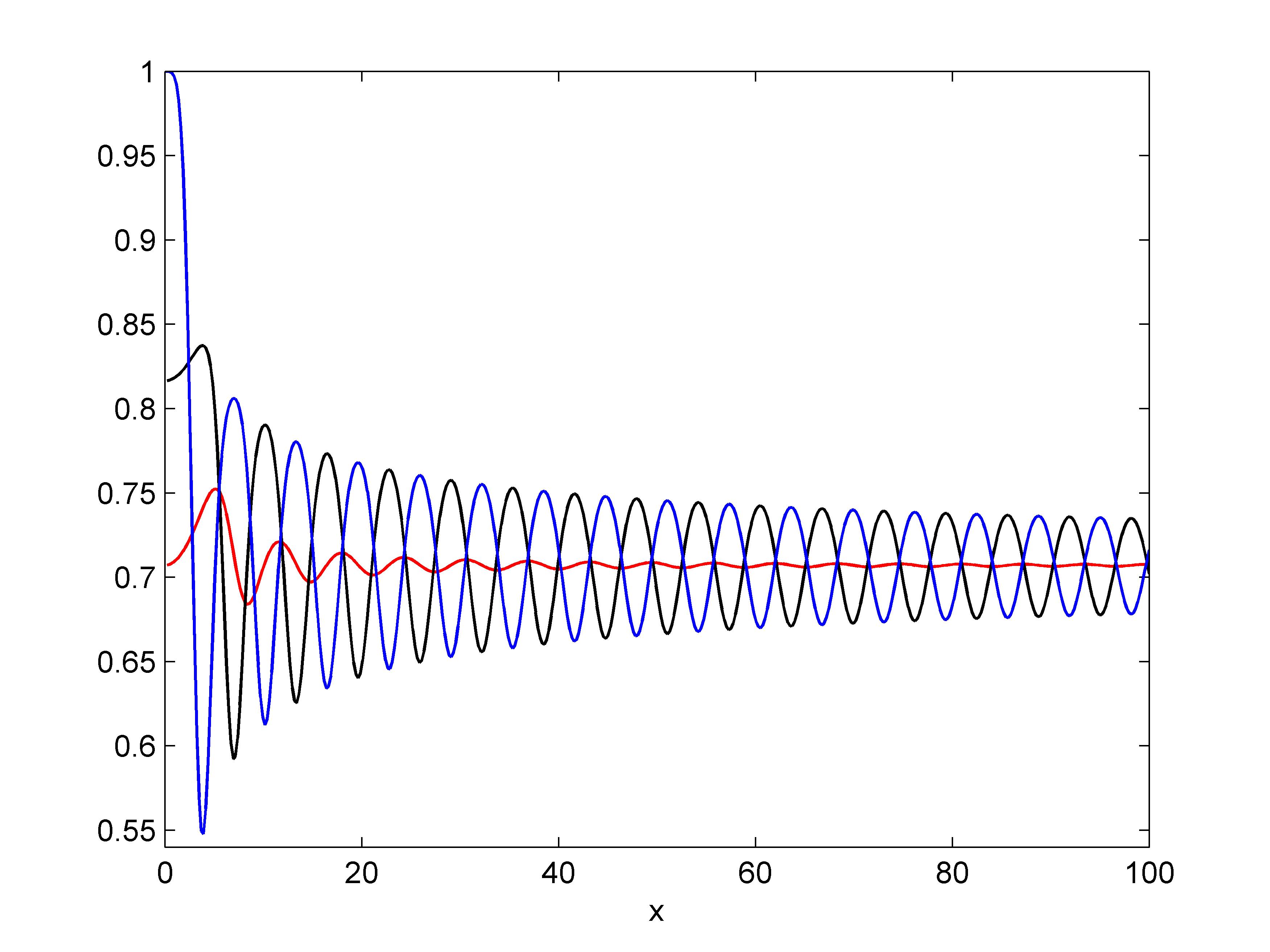
Figure 1. Graphs of the functions (3.19)–(3.21). See text for details.

However, from the proof of Theorem 2.1 above we know that the critical radius of the embeddings of $i_{n}(S^{2})$ in $\mathbb{R}^{(n+1)^{2}}$ is asymptotic to

$$\min\left\{\inf_{x\in[0,\infty)}f(x),\ \frac{1}{\sqrt{2}}\right\}.$$

On the other hand, we know from (4.9)(4.10) in [6] that, for $n$ odd where we have $\widetilde{i}_{n}(S^{2})\cong S^{2}$ (1.2), the limit is

$$\min\left\{\inf_{x\in[0,\infty)}g(x),\ \inf_{x\in[0,\infty)}h(x),\ \frac{1}{\sqrt{2}}\right\};$$

for $n$ even where the map is an immersion $\tilde{i}_{n}(S^{2})\cong\mathbb{R}P^{2}$, the limit is

$$\min\left\{\inf_{x\in[0,\infty)}g(x),\ \frac{1}{\sqrt{2}}\right\}.$$

It thus immediately follows from the Figure 1 that the asymptotic lower bounds for the critical radii of the embeddings of $S^{2}$ by $i_{n}$ we established here are larger than those for the embeddings $\widetilde{i}_{n}$ treated in [6]. This is consistent with the expectations discussed in the Introduction.

4. Proof of Theorem 2.1 for the general case

The arguments for $S^{2}$ can be generalized to higher dimensions in a straightforward fashion, which we now describe.

The kernel $K_{n}^{d}(x,y)$ of $\mathscr{H}_{\ell\leq n}^{d}$ can now be expressed as [3]

$$K_{n}^{d}(x,y)\ =\ \sum_{\ell=0}^{n}\sum_{j=1}^{k_{\ell}^{d}}\phi_{j}^{\ell}(x)\phi_{j}^{\ell}(y)\ =\ \frac{\pi_{n}^{d}/s_{d}}{{n+d/2\choose n}}P_{n}^{(1+\lambda,\lambda)}(\cos\Theta(x,y)),$$

for $x,y\in S^{d}$, where $\lambda=\frac{d-2}{2}$. We first note that [2],

$$P_{n}^{(1+\lambda,\lambda)}(1)\ =\ {n+d/2\choose n}\ =\ \frac{\Gamma(n+d/2+1)}{\Gamma(n+1)\Gamma(d/2+1)};$$

and

$$\ P_{n}^{(1+\lambda,\lambda)^{\prime}}(1)\ =\frac{n+d}{2}{n+d/2\choose n-1}.$$

We define the normalized spectral projection kernel as

$$\Pi_{n}^{d}(x,y)\ =\ \frac{s_{d}}{\pi^{d}_{n}}K_{n}^{d}(x,y)\ =\ {n+d/2\choose n}^{-1}P_{n}^{(1+\lambda,\lambda)}(\Theta(x,y)).$$

Thus the norm of the map (2.4) is $\|i_{n}^{d}(x)\|^{2}=\Pi_{n}^{d}(x,x)=1$, i.e.,

(4.1) $$i_{n}^{d}:\,\,\,S^{d}\to S^{\pi_{n}^{d}-1}.$$

Following the arguments of [6], the pull-back of the Euclidean metric is

(4.2) $$(i_{n}^{d})^{*}(g_{E})\ =\ {n+d/2\choose n}^{-1}P_{n}^{(1+\lambda,\lambda)^{\prime}}(1)g_{S^{d}}\ =\ \frac{n(n+d)}{d+2}g_{S^{d}}.$$

Following the computations in [6], the critical radius of the embedding is

$$\inf_{\theta\in[0,\pi]}\frac{1-{n+d/2\choose n}^{-1}P_{n}^{(1+\lambda,\lambda)}(\cos\theta)}{\sqrt{2-2{n+d/2\choose n}^{-1}P_{n}^{(1+\lambda,\lambda)}(\cos\theta)-{n+d/2\choose n}^{-1}\frac{[P_{n}^{(1+\lambda,\lambda)^{\prime}}(\cos\theta)\sin\theta]^{2}}{P_{n}^{(1+\lambda,\lambda)^{\prime}}(1)}}}.$$

We still have the following classical asymptotic estimate about the Jacobi polynomials. Firstly, we have the asymptotic formula of Hilb’s type below ([9], Theorem 8.21.12):

(4.3) $$\begin{split}P_{n}^{(\alpha,\beta)}(\cos\theta)&\ =\ \left(\sin\frac{\theta}{2}\right)^{-\alpha}\left(\cos\frac{\theta}{2}\right)^{-\beta}\\ &\qquad\times\left\{N^{-\alpha}\frac{\Gamma(n+\alpha+1)}{n!}\left(\frac{\theta}{\sin\theta}\right)^{\frac{1}{2}}J_{\alpha}(N\theta)+R_{1,n}(\theta)\right\},\end{split}$$

where $N=n+(\alpha+\beta+1)/2$,

(4.4) $$R_{1,n}(\theta)\ =\ \begin{cases}\theta^{\alpha+2}O(n^{\alpha}),&0\leq\theta\leq c/n,\\ \theta^{\frac{1}{2}}O(n^{-\frac{3}{2}}),&c/n\leq\theta\leq\pi-\epsilon,\\ \end{cases}$$

and $c,$ $\epsilon$ are uniform constants, independent of $n$. In our case $\alpha=1+\lambda$ and $\beta=\lambda$.
On the subinterval $c^{\prime}/n\leq\theta\leq\pi-c^{\prime}/n$, another asymptotic estimate is given by the Darboux formula ([9], Theorem 8.21.13)

(4.5) $$P_{n}^{(1+\lambda,\lambda)}(\cos\theta)\ =\ \frac{1}{\sqrt{n}}k(\theta)\cos((n+\lambda+1)\theta+\gamma)+R_{2,n}(\theta),$$

where $c$ is a large enough, but uniform, constant, $\gamma=-(\lambda+{3}/{2}){\pi}/{2}$ and

$$k(\theta) = \frac{1}{\sqrt{\pi}}\left(\sin\frac{\theta}{2}\right)^{-\lambda-3/2}\left(\cos\frac{\theta}{2}\right)^{-\lambda-1/2},$$

$$R_{2,n}(\theta) = \frac{1}{\sqrt{n}}k(\theta)\frac{1}{n\sin\theta}O(1).$$

Near the end points, the asymptotic behavior of the Jacobi polynomials is given by the Mehler-Heine formulas ([9], p. 192)

$$\lim_{n\to\infty}n^{-1-\lambda}P_{n}^{(1+\lambda,\lambda)}\left(\cos\frac{x}{n}\right) = \left(\frac{x}{2}\right)^{-1-\lambda}J_{1+\lambda}(x),$$

$$\lim_{n\to\infty}n^{-\lambda}P_{n}^{(1+\lambda,\lambda)}\left(\cos\left(\pi-\frac{x}{n}\right)\right) = \left(\frac{x}{2}\right)^{-\lambda}J_{\lambda}(x),$$

where the limits are uniform on compact subsets of $\mathbb{R}$ and the $J_{\nu}$ are Bessel functions of the first kind with order $\nu$.

Again, following the arguments in Section 3.3, the global infimum is derived by breaking the argument up into the same four subintervals used in the two-dimensional case and given in (3.11).

Using the estimates given above, one can then argue as for the two-dimensional case. This leads to the following lower bound for the critical radius, as $n\to\infty$:

$$\inf_{[0,\infty]}\frac{1-\left(\frac{x}{2}\right)^{-d/2}J_{d/2}(x)}{\sqrt{2-\left(\frac{x}{2}\right)^{-d/2}J_{d/2}(x)-2\Gamma(\frac{d}{2}+2)\left(\left(\left(\frac{x}{2}\right)^{-d/2}J_{d/2}(x)\right)^{\prime}\right)^{2}}}.$$

Again the expression does not diverge at $x=0$, as follows by considering the full expansion of the Bessel function around $0$. This completes the proof of Theorem 2.1 for the general case. ∎

References

- [1] R.J. Adler; J.E. Taylor, Random Fields and Geometry. Springer Monographs in Mathematics. Springer, New York, 2007.
- [2] K. Atkinson; W. Han, Spherical Harmonics and Approximations on the Unit Sphere: An Introduction, Lecture Notes in Mathematics, Volume 2044, 2012, Springer.
- [3] C. Beltran; J. Marzo; J. Ortega-Cerda, Energy and discrepancy of rotationally invariant determinantal point processes in high dimensional spheres. J. Complexity 37 (2016), 76-109.
- [4] M.V. Berry, Regular and irregular semiclassical wavefunctions, J. Phys. A, 10, (1977), no 12, 2083–2091.
- [5] D. Cheng; Y. Xiao, Excursion probability of Gaussian random fields on sphere, Bernoulli 22 (2016), no. 2, 1113-1130.
- [6] R. Feng; R.J. Adler, Critical radius and supremum of random spherical harmonics, arXiv:1702.02767.
- [7] E. Potash, Euclidean embeddings and Riemannian Bergman metrics. J. Geom. Anal. 26 (2016), no. 1, 499-528.
- [8] M. A. Shubin, Pseudodifferential Operators and Spectral Theory, Springer, Berlin (2001).
- [9] G. Szegö, Orthogonal Polynomials, in: American Mathematical Society, vol. 23, Colloquium Publications, 1939.
- [10] Jiayang Sun, Tail probabilities of the maxima of Gaussian random fields, Ann. Probab. Volume 21, Number 1 (1993), 34-71.
- [11] A. Takemura; S. Kuriki, On the equivalence of the tube and Euler characteristic methods for the distribution of the maximum of Gaussian fields over piecewise smooth domains. Ann. Appl. Probab. 12 (2002), no. 2, 768-796.
- [12] S. Vadlamani; D. Marinucci, High frequency of asymptotics of excursion probabilities of spherical random fields, Ann. of Applied Probab., 26(1) (2016), 462-506.
- [13] B. Xu, Derivatives of the spectral function and Sobolev norms of eigenfunctions on a closed Riemannian manifold. Anal. of Global. Anal. and Geom., (2004) 231-252.
- [14] S. Zelditch, Local and global analysis of eigenfunctions on Riemannian manifolds. A survey on eigenfunctions for the Handbook of Geometric Analysis, no. 1: L. Ji, P. Li, R. Schoen and L. Simon(eds.), 14 (2009), 321.