Dynamics of the vortex line density in superfluid counterflow turbulence

Abstract

Describing superfluid turbulence at intermediate scales between the inter-vortex distance and the macroscale requires an acceptable equation of motion for the density of quantized vortex lines ${\mathcal{L}}$. The closure of such an equation for superfluid inhomogeneous flows requires additional inputs besides ${\mathcal{L}}$ and the normal and superfluid velocity fields. In this paper we offer a minimal closure using one additional anisotropy parameter $I_{l0}$. Using the example of counterflow superfluid turbulence we derive two coupled closure equations for the vortex line density and the anisotropy parameter $I_{l0}$ with an input of the normal and superfluid velocity fields. The various closure assumptions and the predictions of the resulting theory are tested against numerical simulations.

I Introduction

The experimental study of the statistical properties of mechanically excited ⁴He superfluid turbulence was somewhat stalled by a realization that these statistics, when observed on large spatial scales, do not differ much from the statistics of the classical counterpart tabeling98 . These results could mean that the two-fluid model of superfluid turbulence may suffice to predict the statistical characteristics of superfluid turbulence. On the other hand, even earlier work on counterflow turbulence Vinen1957 , showed very definitely that on scales that are intermediate between the inter-vortex distances $\ell$ and the outer scale $L$ the observed physics is influenced dramatically by vortex dynamics, vortex reconnections, Kelvin waves on the individual vortex lines, or in short, those effects that exist due to the quantization of vorticity in quantum fluids. These findings underline the difference between “co-flowing” situations (in which the normal and super components average flow is in the same direction) from “counter-flowing” situations. Evidently, a fuller understanding of the statistical theory of “counterflow” superfluid turbulence on these interesting scales calls for deriving an equation for the relevant characteristics of the tangle of quantized vortices which is ubiquitous in this type of turbulence. Indeed, the search for an equation of one of these characteristics, i.e. the density of vortex lines ${\mathcal{L}}$, has been long, starting with the seminal papers of Vinen from the nineteen fifties Vinen1957 . The context in which this equation was studied was that of “counterflow” turbulence in which ⁴He at temperatures below the $\lambda$-point is put in a channel with a temperature gradient, such that the mean normal velocity ${\bm{V}}_{n}$ is directed from the hot to the cold end while the mean superfluid velocity ${\bm{V}}_{s}$ is directed oppositely. The difference between these two mean velocities was denoted as ${\bm{V}}_{\rm ns}$ and the equation that was proposed by Vinen may be written as:

$$\frac{d{\mathcal{L}}}{dt}=\alpha C_{1}|{\bm{V}}_{\text{ns}}|{\mathcal{L}}^{3/2}-\alpha C_{2}\kappa{\mathcal{L}}^{2}\ ,$$ (1)

where $C_{1}$ and $C_{2}$ are dimensionless coefficients, $\alpha$ is known as the “mutual friction parameter” and $\kappa\approx 0.001\rm{cm^{2}/s}$ is the quantum of circulation. Remarkably, this equation which was not derived from first principles, and which was explicitly assumed to apply to homogeneous isotropic situations, has been employed for almost 60 years, becoming the only widely accepted and used equation in the field. Admittedly, Vinen himself expressed concerns whether this equation may apply to inhomogeneous situations Vinen1957 , and in subsequent work attempts have been made to generalize this equation, but no conclusive results were obtained. To find out more about the history of the problem see the review paper Nemirovskii2013 and references therein.

The next important step was the work of Schwarz Schwarz1988 who applied vortex filament method to quantum turbulence to derive an equation for the vortex line density from microscopic principles, but it also underlined the closure problem that results from this approach. Additional and more complicated characteristics of the vortex tangle pop up from the derivation. The two most important objects that appear naturally are the mean curvature and the anisotropy of the vortex tangle. Accordingly, finding an acceptable equation for ${\mathcal{L}}$ for general flows becomes a challenge of finding a reasonable closure in terms of variables that can be measured to compare observations with theory.

A serious hindrance to the completion of this program was the lack of sufficient data to provide verification of possible theories. This hindrance began to lift recently with the advent of numerical simulations. Lipniacki Lipniacki2001 proposed to complement the equation for vortex line density with a coupled equation for the anisotropy parameter in the context of homogeneous but time dependent counterflow turbulence. Further improvement of numerical simulations made it possible to study inhomogeneous counterflow turbulence in a channel Khomenko2015 ; Khomenko2016c ; Baggaley2014 ; Yui2015 . In our own work Khomenko2015 we suggested a new form of the equation for ${\mathcal{L}}$ in a channel which started some discussion in the literature Nemirovskii16 ; Khomenko2016c . The present work is a continuation and an extension of Ref. Khomenko2015 . Here we present a new derivation of an equation for the anisotropy parameter which generalizes and complements our previous results. In our work we opt to focus on steady inhomogeneous flow, in contrast to Ref. Lipniacki2001 which considered homogeneous unsteady flow. We should state at this point that the derivations presented below are not mathematically rigorous. They are based on arguments and estimates. Whenever we can we supplement the analytic arguments with numerical tests. The state of the art of numerical simulations of quantum fluids is not sufficient to nail all the assumption made with certainty. So the reader is advised to consider the present paper as a statement of the state of the art which is possibly not final. More careful work is needed to reach final conclusions. Nevertheless the use of numerical simulations allows us to directly check and verify some crucial assumptions; this fundamentally distinguishes our work from some of the previous papers in this fieldJou2011 .

The structure of this paper is as follows: in Sect. II we review the derivation of the equation of the density of vortex lines and explain how closure bring up the necessity to study new objects like the anisotropy parameter. In Sect. III we derive the equation for anisotropy parameter. A discussion and conclusions are offered in Sect. IV. The appendix provides those technical details that are not given explicitly in the text.

II equation for the density of vortex lines

The starting point for the derivation of an equation of motion of the density of vortex lines is the microscopic equation for a single vortex line Schwarz1988 . Denote by $\bm{s}(\xi,t)$ a given point in space that belongs to a vortex line which is parameterized by the arc-length $\xi$. The one writes the equation

$$\frac{d{\bm{s}}(\xi,t)}{dt}={\bm{V}}_{s}+{\bm{V}}_{\scriptscriptstyle\rm{BS}}({\bm{s}},t)+(\alpha-\tilde{\alpha}\bm{s}^{\prime}\times\big{)}\mathbf{s}^{\prime}\times{\bm{V}}_{\text{ns}}({\bm{s}},t)\,.$$ (2)

Here ${\bm{V}}_{\scriptscriptstyle\rm{BS}}({\bm{s}},t)$ is the velocity generated by the entire vortex tangle, the prime means a derivative along an arc length $d/d\xi$ and $\alpha$ and $\tilde{\alpha}$ are mutual friction parameters. From this equation we can calculate rate of elongation of the vortex line segment $\delta\xi$:

$$\frac{1}{\delta\xi}\frac{d\delta\xi}{dt}=\bm{s}^{\prime}\cdot\frac{d\bm{s}^{\prime}}{dt}\ .$$ (3)

Integrating Eq. (3) over the vortex tangle provides the change in the density of vortex lines ${\mathcal{L}}$. Note that in inhomogeneous condition this wanted equation has the general form:

$$\frac{\partial{\mathcal{L}}}{\partial t}+{\bm{\nabla}}\cdot{\mathcal{J}}_{{\mathcal{L}}}={\mathcal{P}}_{{\mathcal{L}}}-{\mathcal{D}}_{{\mathcal{L}}}\ .$$ (4)

where ${\mathcal{J}}_{{\mathcal{L}}}$ is the flux of the vortex line density, ${\mathcal{P}}_{{\mathcal{L}}}$ is the rate of production and ${\mathcal{D}}_{{\mathcal{L}}}$ the rate of decay of the said density. In the appendix and in Refs.  Khomenko2015 ; Khomenko2016c it is shown that in a channel geometry where the mean flow is in the $x$-direction and the wall normal direction is $y$ one can derive the approximate equations

$${\mathcal{J}}_{{\mathcal{L}}} = \int\left[\frac{d\bm{s}}{dt}\right]_{y}d\xi\approx-\frac{\alpha}{\kappa}V_{\text{ns}}\frac{dV_{\text{s}}}{dy}\ ,$$ (5a)

$${\mathcal{P}}_{{\mathcal{L}}} \approx \alpha\bm{V}_{\text{ns}}\cdot\bm{I}_{l0}\left\langle\varkappa\right\rangle{\mathcal{L}}\ ,$$ (5b)

$${\mathcal{D}}_{{\mathcal{L}}} = \alpha\beta\left\langle\varkappa^{2}\right\rangle{\mathcal{L}}\ .$$ (5c)

Here $$\varkappa\equiv|s^{\prime\prime}| \bm{I}_{l0}$$ is the curvature of the vortex line and the dimensionless vector is defined by:

$$\bm{I}_{l0}=\left\langle\bm{b}\right\rangle,\,\bm{b}=\bm{s}^{\prime}\times\bm{s}^{\prime\prime}/\varkappa\ .$$ (5d)

The derivation of these equations is based on the following assumptions:

1. Separation of scales; we assume that the “macroscopic” variable $V_{\text{ns}}$ changes slowly in space in comparison to rate of spatial change of $\bm{s}^{\prime}$ and $\bm{b}$. Accordingly the average of their product can be estimated as a product of the averages.

2. We neglect the term in Eq. (2) proportional to $\tilde{\alpha}$. The reason is that in counterflow conditions this coefficient is much smaller than $\alpha$.

3. We assume that the derivative $dV_{\text{ns}}/d\xi$ along vortex lines is negligible on the average.

Equations (5) expose the appearance of new fields, i.e. the objects $\left\langle\varkappa\right\rangle,\left\langle\varkappa^{2}\right\rangle$ and $\bm{I}_{l0}$. To be able to close the system of equations these objects should be either expressed in terms of known variables (${\mathcal{L}}$, $V_{\text{ns}}$, …) or supplemented by equations for the new objects.

To proceed, another fundamental assumption is called for. We assert that there exists only one typical length-scale in the problem which is inter-vortex distance. Therefore the radius of curvature should be proportional to it. This is a closure relation that reads $\left\langle\varkappa\right\rangle\simeq c_{1}{\mathcal{L}}^{1/2}$. This assumption is expected to be reasonable for relatively low gradients of counterflow velocity. We tested it and found that it works well for parabolic profiles of the normal velocity in the case of T1 turbulence in a channel, cf. Ref. Khomenko2015 .

The closure of $I_{l0}$ is more complicated. In Ref. Khomenko2015 , in analogy with the Vinen equation, we assume that $I_{l0}$ can be expressed in terms of $V_{\text{ns}}$ and ${\mathcal{L}}$ only. Being dimensionless, it must be a function of the dimensionless variable $\zeta=V_{\text{ns}}/(\kappa{\mathcal{L}}^{1/2})$. Based on numerical experiments we concluded that taking $I_{l0}\propto\zeta^{2}$ gives a good match for all the available data obtained by simulations in a channel. Below we generalize this to other geometries. With these explicit assumptions one obtains the closure for Eq. (5c):

$${\mathcal{J}}_{{\mathcal{L}}} \approx -\frac{\alpha}{\kappa}V_{\text{ns}}\frac{dV_{\text{s}}}{dy}\,,$$ (6a)

$${\mathcal{P}}_{{\mathcal{L}}} \approx \alpha C_{\text{prod}}V_{\text{ns}}^{3}\sqrt{{\mathcal{L}}}/\kappa^{2}\,,$$ (6b)

$${\mathcal{D}}_{{\mathcal{L}}} \approx \alpha\beta C_{\text{dec}}{\mathcal{L}}^{2}\ .$$ (6c)

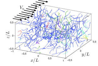
Figure 1: Sketch of the computational setup.

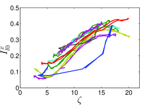
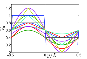
Figure 2: Upper panel: examples of imposed normal velocity profiles in the simulation channel. Lower panel: parametric plot $[\zeta(y),I^{x}_{l0}(y)]$ of the stream-wise projection of the anisotropy parameter.

III Equation for the anisotropy parameter

Admittedly, while the closure for $I_{l0}$ matches well with the available numerical results for T1 counterflow turbulence in the channel, its derivation did not provide adequate physical intuition or an explanation why it gave a good agreement with the data. Accordingly it is not clear how general this closure is. To test the limits of its applicability we did a series of additional numerical simulations with various different profiles of the normal velocity shown in the upper panel of Fig. 1. The simulations were performed using the full Biot-Savart calculation, employing vortex filament methods as explained in detail in Ref. Kondaurova2014 . Using periodic boundary conditions , we have a greater freedom of choice for the normal velocity profile. The simulations were carried out in a computational box of size $2L\times L\times L,L=0.1$ cm with 3-periodic boundary conditions (cf. Fig1) for $T=1.6\,$K and $V_{\text{n}}=(0.4\div 1.0)$ cm/s. In all these simulations we measured the anisotropy parameter $I_{l0}$ and plotted the results in the lower panel of Fig. 2 as a parametric plot $[I_{l0}(y),\zeta(y)]$. The results convey the clear message that $I_{l0}$ is not a function of $\zeta$ only. Additional dimensionless variables in addition to $\zeta$ appear to be necessary. Candidates are for example

$$\zeta_{2}=\frac{1}{\kappa{\mathcal{L}}}\frac{dV_{s}}{dy}\,,\quad\zeta_{3}=\frac{1}{\kappa{\mathcal{L}}^{3/2}}\frac{d^{2}V_{s}}{dy^{2}}\,,\dots$$ (7)

As a test of this conclusion we show in Fig. 3 the results of allowing the anisotropy parameter to depend on two variables, i.e. $\zeta$ and $\zeta_{2}$. An improvement in the data representation is evident. To find the two-variable parametric surface, we used general polynomial and Padé approximants. The resulting mean square deviation was reduced by 50 % compared to the fit that depended on $\zeta$ only. Accordingly we turn now to a derivation based on microscopic relations.

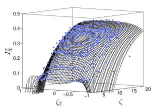
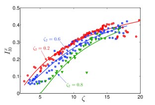
Figure 3: Parametric plot of $[\zeta(y),\zeta_{2}(y),I_{l0}(y)]$ for all the normal velocity profiles shown in Fig. 2. Upper Panel: The surface embedded in 3-dimensions which spans all the available data points. Lower Panel: $I_{l0}(y)$ as a function of $\zeta$ for different values of $\zeta_{2}$, as marked in the plot. Points are data from all the simulations for $\zeta_{2}=0.2\pm 0.1$ (red), $0.6\pm 0.1$ (blue), $0.8\pm 0.1$ (green). Lines of corresponding colors denote the fit [cf the surface shown in the Upper Panel].

III.1 Derivation based on microscopic relations

To find an expression for the anisotropy parameter $I_{l0}$ in a systematic way we will derive its equation of motion. We start again from Eq. (2). In the appendix we show that applying this equation to the unit vector $\bm{b}$ we get:

$$\frac{d\bm{b}}{dt}=\alpha\varkappa\bm{V}_{\rm ns}^{0}-\alpha\varkappa\left(\bm{b}\cdot\bm{V}_{\rm ns}^{0}\right)\bm{b}+\beta\tau^{2}\bm{s}^{\prime\prime}/\varkappa\ ,$$ (8)

where $\tau$ is a torsion of the vortex line. This equation can be rewritten in the following form:

$$\frac{d\bm{b}}{dt}=\alpha\varkappa\bm{b}\times\left(\bm{V}_{\rm ns}^{0}\times\bm{b}\right)+\beta\tau^{2}\bm{s}^{\prime\prime}/\varkappa\ .$$ (9)

Note that Eq. (9) is very similar to the equation for vortex rings that was used in Ref. Lipniacki2001 for $I_{l0}$ in a homogeneous flow. In an inhomogeneous and anisotropic flow the equation satisfied by $I_{l0}$ will again have a production term denoted as ${\mathcal{P}}_{I_{l0}}$, a decay term, denoted as ${\mathcal{D}}_{I_{l0}}$, and a flux term denoted as $\bm{{\hat{{\mathcal{J}}}}_{I_{l0}}}$. Two of these can be obtained easily. Integrating Eq. (8) over the tangle provides the production term for $I_{l0}$. The flux term can also be found analytically,

$$\bm{{\hat{{\mathcal{J}}}}_{I_{l0}}}=\Big{\langle}\frac{d\bm{s}}{dt}\otimes\bm{b}\Big{\rangle}\ .$$ (10)

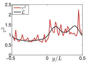
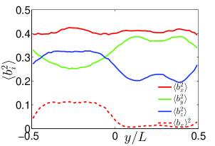
Figure 4: Upper panel: the profiles of $\tau^{2}(y)$ and the normalized density of vortex lines ${\mathcal{L}}(y)/\langle{\mathcal{L}}\rangle$, plotted for the sine-like normal velocity profile. Lower panel: the corresponding profiles of $\left\langle b_{i}^{2}\right\rangle$ and $\left\langle b_{i}\right\rangle^{2}$.

The last ingredient, the decay, is governed by the effect of vortex reconnection. This term is difficult to derive from the microscopic equation and at this point it can only be written down phenomenologically. The effect of vortex reconnection is to locally form sharp tips Buttke98 ; TYB11 ; ZCBB12 ; Boue2013 that can be oriented in any spatial direction which is determined by the relative orientation of the two reconnecting vortex lines. This tends to destroy any pre-orientation of the vortex lines. Based on this picture we can assume that in each event of reconnection a region which is affected by it will loose its anisotropy $I_{l0}$. Phenomenologically we can write the decay due to reconnections in the following way:

$${\mathcal{D}}_{I_{l0}}\approx\frac{C}{\left\langle\varkappa\right\rangle{\mathcal{L}}}\frac{dN_{\text{rec}}}{dt}I_{l0}\ .$$ (11)

Here $dN_{\text{rec}}/dt$ is the reconnection rate, $1/\varkappa$ is the radius of curvature which defines the region affected by the reconnection event and $I_{l0}$ is the value of anisotropy that was lost during the reconnection.

Now that all the necessary objects are expressed in terms of macroscopic fields, we recognize that ones more there appeared new quantities, i.e. $\langle b_{x}^{2}\rangle$, $\tau^{2}$ and $dN_{\text{rec}}/dt$ that should be modeled. We will start with torsion. Torsion is a second curvature and we expect that the radius of torsion would be proportional to the inter-vortex distance:

$$\left\langle\tau^{2}\right\rangle\approx C_{\tau}{\mathcal{L}}\ .$$ (12)

Note that this assumption is similar to the previously performed closure for the curvature $\varkappa$ and is expected to have similar validity. Unfortunately at present we can not test this assumption numerically due to the insufficient accuracy of our simulations. Nevertheless preliminary results shown in the upper panel of Fig. 3 look promising. Regarding the object $\left\langle b_{x}^{2}\right\rangle$ there are two limiting cases that could be considered: (i) strongly polarized tangle: in this case $\left\langle b_{x}^{2}\right\rangle\approx\left\langle b_{x}\right\rangle^{2}$; (ii) a fully isotropic case: $\left\langle b_{x}^{2}\right\rangle\approx 1/3$. Based on the results of many numerical simulation we can say that in the case of counterflow turbulence (T1 regime) we are closer to the second case, and even though $\left\langle b_{x}^{2}\right\rangle$ is slightly larger than $(\left\langle b_{y}^{2}\right\rangle+\left\langle b_{y}^{2}\right\rangle)/2$, it can be considered as a constant with reasonable accuracy,

$$\left\langle b_{x}^{2}\right\rangle\approx\mbox{const.}$$ (13)

Evidence is provided in the lower panel of Fig. 4.

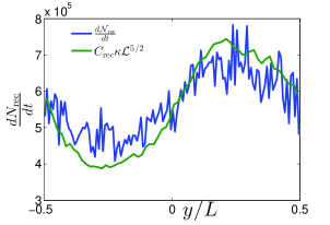
Figure 5: The profile of the reconnection rate and its estimate via the closure discussed in the text. In this example the imposed normal velocity profile is sine-like.

The last object is the vortex reconnection rate. Motivated by dimensional reasoning and supported by results from homogeneous turbulence Barenghi2004 ; Nemirovskii2006 , we can model the reconnection rate profile by:

$$\frac{dN_{\text{rec}}}{dt}\approx C_{\text{rec}}\kappa{\mathcal{L}}^{5/2}\ .$$ (14)

The numerical data presented in Fig. 5 support this conclusion and see also the results in Ref. Baggaley2014 .

III.2 Putting things together

Summarizing together all the discussed results we end up with a system of equations:

$$\frac{\partial I_{l0}}{\partial t}+\frac{\partial{\mathcal{J}}_{I_{l0}}}{\partial y}={\mathcal{P}}_{I_{l0}}-{\mathcal{D}}_{I_{l0}}\,,$$ (15a)

$${\mathcal{J}}_{I_{l0}} \approx \frac{1}{{\mathcal{L}}}\Big{(}-\frac{\alpha}{\kappa}V_{\text{ns}}\frac{dV_{\text{s}}}{dy}I_{l0}+C\beta\frac{dV_{s}}{dy}\Big{)}\,,$$ (15b)

$${\mathcal{P}}_{I_{l0}} \approx \alpha C_{1}V_{\text{ns}}{\mathcal{L}}^{1/2}+C_{2}\frac{\beta}{{\mathcal{L}}}\frac{d^{2}V_{s}}{dy^{2}}\,,$$ (15c)

$${\mathcal{D}}_{I_{l0}} \approx C_{\text{dec}}\kappa{\mathcal{L}}I_{l0}\ .$$ (15d)

Note that in Eq. (15b) we used results from Ref. Khomenko2016b to model $\left\langle s^{\prime\prime}\right\rangle$.

IV Discussion and conclusions

The central result of this paper is the equation of motion for anisotropy parameter $I_{l0}$; we showed that it is possible to close it in terms of known variables. Together with the equation for the density of vortex lines we possess now a set of equations that allows a calculation of the profile of the anisotropy parameter and the vortex line density self-consistently, relaxing the assumption on the production term made in Ref.Khomenko2015 . The approach described above has pros and cons. On the negative side, we recognize that a number of new assumptions were made whose verification is currently beyond our computational capabilities. Of particular concern is the phenomenological model for the anisotropy decay due to reconnections, and the precise modeling of the torsion and the flux of $I_{l0}$. On the positive side the work described above prepares a theoretical background for future numerical simulations. It underlines the missing links in our current understanding of the subject. Moreover, even on the basis of what is known now we have enough information from numerical simulations to afford making simplifications that are relevant for the study of counterflow turbulence. Finally, possible future experiments in inhomogeneous and anisotropic superfluid flows should also be carefully designed and analyzed to shed further light on the issues discussed above. Indeed, a proper description of the physics of vortex lines requires knowledge of both the vortex line density and the anisotropy of the vortex tangle; the measurement of at least two different fields is needed. For example, one can use the fact that the attenuation of second-sound depends on the angle between its propagation direction and the vortex line direction Babuin12 . Thus, measuring the attenuation along two orthogonal directions one can extract the total line density as well as information about the the anisotropy of the vortex tangle. Probably even more informative would be experiments of a counterflow and pure superflow in a rectangular channel with a large aspect ratio measuring the second sound attenuation, propagating in all three directions. This type of experiments, possibly combined with visualization techniques, may expand our understanding of counterflows in superfluid ⁴He, and in particular, shed light on the importance of the vortex tangle anisotropy.

Appendix A Microscopic Derivations

A.1 Equation for the density of vortex lines.

We will start from Eqs. (2) and Eq. (3):

$$\frac{1}{\delta\xi}\frac{d\delta\xi}{dt}=\alpha\bm{V}_{\text{ns}}({\bm{s}},t)\cdot({\bm{s}}^{\prime}\times{\bm{s}}^{\prime\prime})+{\bm{s}}^{\prime}\cdot{{\bm{V}}_{\text{nl}}^{s}}^{\prime}-\tilde{\alpha}{\bm{s}}^{\prime\prime}\cdot{\bm{V}}_{\text{ns}}\ .$$ (16)

The first simplification that we make is neglecting the term proportional to $\tilde{\alpha}$. This simplification is justifiable for temperatures higher than T=1.3 K when $\tilde{\alpha}$ much smaller than $\alpha$, but might be reconsidered for lower temperatures. Second, we can argue that the second term on the RHS of Eq. (16) is in fact negligible. To see this note that ${\bm{V}}_{\text{nl}}$ is a macroscopic field that changes slowly on the length-scale of inter-vortex distance. For the present flow which is inhomogeneous in the $y$-direction, we note that due to symmetry all the average values depend only on the y-coordinate, and their only non-zero component is in the x-direction. In contrast, $\left\langle s^{\prime}_{y}\right\rangle=\left\langle s^{\prime}_{x}\right\rangle=0$. Together this is a strong reason to assert that this term is negligible compared to the first term in Eq. (16). Indeed in our numerical simulations we could confirm this assertion, cf. Ref. Khomenko2016c .

Next we can decompose the counterflow velocity $V_{\text{ns}}$ into a local $-\beta\bm{s}^{\prime}\times\bm{s}^{\prime\prime}$ and slowly-varying nonlocal $V_{\text{ns}}^{0}$ components:

$$\frac{1}{\delta\xi}\frac{d\delta\xi}{dt}\approx\alpha V_{\text{ns}}^{0}\cdot({\bm{s}}^{\prime}\times{\bm{s}}^{\prime\prime})-\alpha\beta|s^{\prime\prime}|^{2}\ .$$ (17)

Integrating this equation over the tangle results in an equation for the production and decay of the vortex line density:

$${\mathcal{P}}_{{\mathcal{L}}} = \frac{\alpha}{\Omega}\int{\bm{V}}_{\text{ns}}^{0}\cdot({\bm{s}}^{\prime}\times{\bm{s}}^{\prime\prime})d\xi\approx\alpha{\mathcal{L}}\left\langle\varkappa\right\rangle V_{\text{ns}}\cdot\left\langle b\right\rangle\,,~{}~{}~{}~{}~{}~{}$$ (18)

$${\mathcal{D}}_{{\mathcal{L}}} = \frac{1}{\Omega}\int\alpha\beta|s^{\prime\prime}|^{2}d\xi\approx\alpha\beta{\mathcal{L}}\left\langle\varkappa^{2}\right\rangle\ .$$ (19)

A.2 The flux of the vortex lines density

The flux of the density of vortex lines is defined by:

$$\bm{\mathcal{J}}_{{\mathcal{L}}}=\Big{\langle}\frac{d\bm{s}}{dt}\Big{\rangle}\ .$$ (20)

In the considered geometry only the $y$-component survives:

$$[{\mathcal{J}}_{{\mathcal{L}}}]_{y}\approx\left\langle\alpha s^{\prime}_{z}V_{\text{ns}}\right\rangle\approx\alpha\left\langle s^{\prime}_{z}\right\rangle V_{\text{ns}}=-\frac{\alpha}{\kappa}V_{\text{ns}}\frac{dV_{\text{s}}}{dy}\ .$$ (21)

Note that in general the vortex flux can also contain other terms Khomenko2016c , for example a diffusive component Tsubota2003 ; Nemirovskii2010 ; however if the tangle is polarised, as in the case of counterflow or rotating turbulence, these terms are expected to be negligible. Nevertheless, in particular geometriesSaluto16 they may become important.

A.3 The equation for the anisotropy parameter

We start from Eq. (2) after discarding the term proportional to $\tilde{\alpha}$:

$$\frac{d\bm{s}}{dt}=\bm{V}_{s}+\alpha\bm{s}^{\prime}\times\bm{V}_{\rm ns}.$$ (22)

The derivative for binormal vector $\bm{s}^{\prime}\times\bm{s}^{\prime\prime}$ reads

$$\frac{d}{dt}(\bm{s}^{\prime}\times\bm{s}^{\prime\prime})=\frac{d\bm{s}^{\prime}}{dt}\times\bm{s}^{\prime\prime}+\bm{s}^{\prime}\times\frac{d\bm{s}^{\prime\prime}}{dt}\ .$$ (23)

Using these equations together gives:

$$\frac{d\bm{missing}}{dt}(\bm{s}^{\prime}\times\bm{s}^{\prime\prime})=\bm{V}_{s}^{\prime}\times\bm{s}^{\prime\prime}+\alpha(\bm{s}^{\prime\prime}\times\bm{V}_{\rm ns})\times\bm{s}^{\prime\prime}$$

$$+\alpha(\bm{s}^{\prime}\times\bm{V}_{\rm ns}^{\prime})\times\bm{s}^{\prime\prime}+\bm{s}^{\prime}\times\bm{V}_{s}^{\prime\prime}+\alpha\bm{s}^{\prime}\times(\bm{s}^{\prime\prime\prime}\times\bm{V}_{\rm ns})$$

$$+2\alpha\bm{s}^{\prime}\times(\bm{s}^{\prime\prime}\times\bm{V}_{\rm ns}^{\prime})+\alpha\bm{s}^{\prime}\times(\bm{s}^{\prime}\times\bm{V}_{\rm ns}^{\prime\prime}).$$ (24)

To express higher derivatives in terms of $\bm{s}^{\prime}$ and $\bm{s}^{\prime\prime}$ we can use the Frenet-Serret formula wiki :

$$\bm{s}^{\prime\prime\prime}=-\varkappa^{2}\bm{s}^{\prime}+\tau\bm{s}^{\prime}\times\bm{s}^{\prime\prime}+\frac{\varkappa^{\prime}}{\varkappa}\bm{s}^{\prime\prime}\ ,$$ (25)

where $\varkappa$ is the curvature and $\tau$ is the torsion. At this point it is advantageous to split $V_{\text{ns}}$ into a local term $-\beta\bm{s}^{\prime}\times\bm{s}^{\prime\prime}$ and a non local term $V_{\text{ns}}^{0}$:

$$\bm{V}_{\text{ns}}=\bm{V}_{\text{ns}}^{0}-\beta\bm{s}^{\prime}\times\bm{s}^{\prime\prime}\ .$$ (26)

If we neglect terms with derivatives of the nonlocal velocity component, we get:

$$\frac{d}{dt}(\bm{s}^{\prime}\times\bm{s}^{\prime\prime})=2\alpha\varkappa^{2}\bm{V}_{\text{ns}}^{0}+\alpha\bm{s}^{\prime}\left[-\beta\varkappa^{2}\tau-\varkappa^{2}(\bm{s}^{\prime}\cdot\bm{V}_{\text{ns}}^{0})\right]$$

$$+\bm{s}^{\prime\prime}\left[\beta\tau^{2}-\alpha(\bm{s}^{\prime\prime}\cdot\bm{V}_{\text{ns}}^{0})\right]-\alpha\beta\left[2\varkappa^{2}+\tau^{2}\right](\bm{s}^{\prime}\times\bm{s}^{\prime\prime})$$ (27)

The next step of simplification is to neglect terms proportional to $\tau$. The torsion, in contrast to the curvature, is not positive definite and we can assume that the mean value of $\tau$ is negligible. Our current numerical simulations are not sufficiently precise to test this assertion, although preliminary results indicate that this assumption is correct.

Now having an equation for $\bm{s}^{\prime}\times\bm{s}^{\prime\prime}$ we can write an equation for the unit vector $\bm{b}$:

$$\frac{d\bm{b}}{dt}=\frac{1}{\varkappa}\left(\frac{d\bm{s}^{\prime}\times\bm{s}^{\prime\prime}}{dt}-\bm{b}\frac{d\bm{s}^{\prime}\times\bm{s}^{\prime\prime}}{dt}\cdot\bm{b}\right)\ .$$ (28)

Substituting $d(\bm{s}^{\prime}\times\bm{s}^{\prime\prime})/dt$:

$$\frac{d\bm{b}}{dt} = \alpha\varkappa\bm{V}_{\rm ns}^{0}-\alpha\varkappa\left(\bm{b}\cdot\bm{V}_{\rm ns}^{0}\right)\bm{b}+\beta\tau^{2}\bm{s}^{\prime\prime}/\varkappa$$ (29)

A.4 Flux of the anisotropy parameter

The flux of the anisotropy parameter $I_{l0}$ can be written as:

$${\hat{\bm{\mathcal{J}}}}_{{\bm{I}}_{l0}}=\Big{\langle}\frac{d\bm{s}}{dt}\otimes\bm{b}\Big{\rangle}\ .$$ (30)

In the channel geometry only the $xy$ component of the tensor survives:

$$[{{\mathcal{J}}}_{I_{l0x}}]_{y}=\Big{\langle}\Big{[}\frac{d\bm{s}}{dt}\Big{]}_{y}b_{x}\Big{\rangle}\approx\langle\beta\varkappa b_{x}b_{y}\rangle+\langle\alpha s^{\prime}_{z}V_{\text{ns}}b_{x}\rangle\ .$$ (31)

The first term is given by local velocity and with a good accuracy can be expressed as:

$$\left\langle b_{x}b_{y}\right\rangle = \left\langle\frac{s^{\prime}_{y}s^{\prime}_{z}s^{\prime\prime}_{z}s^{\prime\prime}_{x}-s^{\prime}_{x}s^{\prime}_{y}{s^{\prime\prime}_{z}}^{2}-{s^{\prime}_{z}}^{2}s^{\prime\prime}_{z}s^{\prime\prime}_{x}+s^{\prime}_{x}s^{\prime}_{z}s^{\prime\prime}_{y}s^{\prime\prime}_{z}}{\varkappa^{2}}\right\rangle$$ (32)

$$\approx -\left\langle s_{x}^{\prime}s_{y}^{\prime}\right\rangle/3\,,$$

while for second term we make the uncontrolled approximation:

$$\langle\alpha s^{\prime}_{z}V_{\text{ns}}b_{x}\rangle\approx\left\langle\alpha s^{\prime}_{z}V_{\text{ns}}^{0}\right\rangle\left\langle b_{x}\right\rangle-\alpha\beta\left\langle s_{z}^{\prime}\right\rangle\left\langle\varkappa b_{x}^{2}\right\rangle\ .$$

This approximation needs to be verified in future numerical simulations.

References

- (1) J. Maurer and P. Tabeling,Local investigation of superfluid turbulence, Europhys. Lett. , 43, 29 (1998)
- (2) W.F. Vinen. Mutual friction in a heat current in liquid helium II. III. Theory of the mutual friction. Proc. R. Soc. Lond. A 242, 493 (1957).
- (3) S. Nemirovskii, Quantum turbulence: Theoretical and numerical problems. Physics Reports, 524, 85 (2013).
- (4) K. W. Schwarz, Three-dimensional vortex dynamics in superfuid 4He: Homogeneous superfluid turbulence. Phys. Rev. B, 38, 2398 (1988).
- (5) T. Lipniacki. Evolution of the line-length density and anisotropy of quantum tangle in He4. Phys. Rev. B, 64 214516 (2001).
- (6) D. Khomenko, L. Kondaurova, V.S. L’vov, P. Mishra, A. Pomyalov, I. Procaccia. Dynamics of the density of quantized vortex lines in superfluid turbulence. Phys. Rev. B. 91,80504(R) (2015).
- (7) S. K. Nemirovskii, Comment on “Dynamics of the density of quantized vortex lines in superfluid turbulence”. Phys. Rev. B 94, 146501 (2016).
- (8) D. Khomenko, V.S. L’vov, A. Pomyalov, and I. Procaccia. Reply to ”comment on ’Dynamics of the density of quantized vortex lines in superfluid turbulence’ ”. Phys. Rev. B ,942, 146502 (2016).
- (9) A. W. Baggaley and J. Laurie. Thermal Counterflow in a Periodic Channel with Solid Boundaries. JLTP, 178, 35 (2014).
- (10) S. Yui and M. Tsubota. Counterflow quantum turbulence of He-II in a square channel: Numerical analysis with nonuniform flows of the normal fluid. Phys. Rev. B 91, 184504 (2015).
- (11) D. Jou, M. Mongioví, M. Sciacca, Hydrodynamic equations of anisotropic, polarized and inhomogeneous superfluid vortex tangles. Physica D, 40, 249 (2011).
- (12) L. Kondaurova, V.S. L’vov, A. Pomyalov, I. Procaccia, Structure of a quantum vortex tangle in He-4 counterflow turbulence. Phys. Rev. B. 89, 014502 (2014).
- (13) T.F. Buttke, Numerical study of superfluid turbulence in the selfinduction approximation, J. Comput. Phys. 76, 301 (1988).
- (14) S. Zuccher, M. Caliari, A. W. Baggaley, and C. F. Barenghi, Quantum vortex reconnections. Phys. Fluids 24, 125108 (2012).
- (15) R. Tebbs, A.J. Youd, C.F. Barenghi, The Approach to Vortex Reconnection, J. Low Temp Phys 162, 314(2011).
- (16) L. Bou´e, D. Khomenko, V.S. L’vov, and I. Procaccia. Analytic solution of the approach of quantum vortices towards reconnection. Phys. Rev. Lett., 111, 145302 (2013).
- (17) C. F. Barenghi and D. C. Samuels. Scaling laws of Vortex Reconnections. JLTP, 136, 281 (2004).
- (18) S. K. Nemirovskii. Evolution of a Network of Vortex Loops in He- II : Exact Solution of the Rate Equation. Phys. Rev. Lett., 96, 015301 (2006).
- (19) D. Khomenko, V. S. L’vov, A. Pomyalov, and I. Procaccia. Mechanical momentum transfer in wall-bounded superfluid turbulence. Phys. Rev. B, 93, 134504 (2016).
- (20) Wikipedia Frenet-Serret formulas, https://en.wikipedia.org/wiki/Frenet
- (21) M. Tsubota, T.Araki, W. Vinen. Diffusion of an inhomogeneous vortex tangle. Physica B, 329-333, 224 (2003).
- (22) S. Nemirovskii. Diffusion of inhomogeneous vortex tangle and decay of superfluid turbulence. Phys. Rev. B, 81, 64512 (2010).
- (23) S. Babuin, M. Stammeier, E. Varga, M. Rotter and L. Skrbek, Quantum turbulence of bellows-driven 4He superflow: Steady state, Phys. Rev. B 86, 134515 (2012).
- (24) L. Saluto, M. S. Mongioví, Inhomogeneous vortex tangles in counterlow superfluid turbulence: flow in convergent channels, Commun. Appl. Ind. Math. 7, 130–149(2016).