Top-Frequency Parallel Coordinates Plots

Abstract

Parallel coordinates plotting is one of the most popular methods for multivariate visualization. However, when applied to larger data sets, there tends to be a “black screen problem,” with the screen becoming so cluttered and full that patterns are difficult or impossible to discern. Xie and Matloff (2014) proposed remedying this problem by plotting only the most frequently-appearing patterns, with frequency defined in terms of nonparametrically estimated multivariate density. This approach displays “typical” patterns, which may reveal important insights for the data. However, this remedy does not cover variables that are discrete or categorical. An alternate method, still frequency-based, is presented here for such cases. We discretize all continuous variables, retaining the discrete/categorical ones, and plot the patterns having the highest counts in the dataset. In addition, we propose some novel approaches to handling missing values in parallel coordinates settings.

Keywords: multidimensional visualization; Big Data; Method of Moments

1 Introduction

The problem of visualizing data of more than three dimensions has vexed analysts throughout the history of “number crunching,” but has become especially acute in today’s era of Big Data. For the common case of $n$ data points, each consisting of $p$ variables/features, Big Data has either $n$ or $p$ large, often both. As noted in Bühlmann et al. (2016), in analyses of Big Data it is useful to distinguish between the large-$p$ and large-$n$ cases. Though discussions of visualizing multidimensional data typically focus on the large-$p$ setting, here we will see that large $n$ can be problematic as well.

One of the most popular approaches has been parallel coordinates plots (PCPs); see e.g. Inselberg (2009) and Unwin et al. (2007). Here one draws $p$ vertical axes, with each data point being represented by a polygonal line connecting nodes on the axes. Denoting data point $i$ by $(X_{i1},...,X_{ip})$, the node at axis $j$ has height $X_{ij}$.

This is simple and satisfying for small values of $n$ and $p$. However, in general it can be a challenge to tease insight out of these fascinating lines. For instance, for $p$ larger than, say, two dozen, there simply is not enough room on a computer screen to view all of the axes at once. Indeed, even if there is sufficent room, it may be difficult to view the relationship of variables that are far apart on the screen. Software packages generally handle this in different ways, allowing the user to permute the columns or even generate a new permutation every few seconds.

With large $n$ there typically is a “black screen problem” (BSP), in which substantial portions of the screen become solid black. For instance, consider the Million Song Dataset in Bertin-Mahieux et al. (2011). One of the available versions has $n=515345$ and $p=91$. The first column of the data is the year in which the song was released, and the remaining data involves technical audio aspects of the song. Even using just a random subsample of 50000 data points, and just every 10th column, we encounter the black screen problem shown in Figure 1 (the R package ggparcoord was used here.)

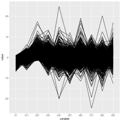
Figure 1: Million song subset, ordinary parallel coordinates

2 Top-Frequency Parallel Coordinates Plots: Continuous-Variables Case

There have been numerous methods proposed for handling the BSP. One approach for instance is to make the printed points more transparent, via alpha blending, as in Unwin et al. (2007). But this merely postpones the problem, as $n$ grows.

Another approach is to draw a random subsample of size $N$ from the data, consisting of say, hundreds or thousands of data points, and then form a PCP from the subsample. This “thinning out” of the data ameliorates the BSP, but even a graph of a few hundred lines may become crowded and difficult to interpret, and there are other issues. We will return to this in Section 7.

By contrast, our approach “thins out” the data in a different way, by using the entire data set but plotting only the most representative points. (For investigating outliers, this becomes plotting the least representative points.)

To see how this works, first consider settings in which the variables are continuous, as opposed to discrete or categorical. In Matloff and Xie (2013b) the third and fourth authors of the present paper proposed plotting only those points having the highest estimated multivariate density, and implemented the method in the CRAN package freqparcoord, Matloff and Xie (2013a). These then are “typical” points, thus hopefully shedding some light on the multivariate relations.

In a sense, this is analogous to cluster hunting, say finding (an unknown number of) components of a Gaussian mixture. Typically in cluster analysis the centroid (vector of means) or medoid (vector of univariate medians) is taken as the anchor of a component; here it is the multivariate mode of the component.

Let us refer to this as Top-Frequency Parallel Coordinates (TFPC). Though we will often be discussing specific software packages here, this paper will treat TFPC as a general method. Throughout this paper, we will use the letter $F$ to denote the number of lines plotted, i.e. we plot the $F$ most-frequent lines.

In freqparcoord the density estimation is performed using k-Nearest Neighbors estimation. To estimate the density of a $q$-dimensional random vector $W$ at a point $t$, based on a sample $W_{1},...,W_{m}$, we first determine

$$D(t)=\max_{W_{i}\textrm{ in }A(t)}\textrm{distance}(W_{i},t)$$ (1)

where $A(t)$ is the set of the $k$ closest sample points to $t$

The density estimate is then

$$\frac{k}{\textrm{vol}(D(t))}$$ (2)

with vol() representing the volume of a hypersphere with radius given in the argument. Since we are simply comparing distances, we can ignore a multiplicative constant in that volume, and simply take the volume to be $\pi^{q}$. The lines plotted are then the ones with the $k$ highest estimated frequencies.

Again, the crucial point is the ‘T’ in “TFPC.” We only plot the most frequently-occurring points, as determined via the density estimation. This is key to avoiding the BSP. By contrast, Wegman (1990) for example proposed plotting entire density estimates, resulting in a shaded graph.

A typical example of TFPC, applied in this case to the song data ($n=50000$, plotting the $F=50$ most frequent lines), is shown in Figure 2. There is a narrow but solid band running through the middle of the jumble of lines. It is lighter gray in monochrome, lighter blue in the color version. Tracing the band back to the first variable, Year, one finds that the band corresponds approximately to years 2004 onward (scaled value about 0.6). This is a good example of what PCPs are supposed to do, culling out unusual patterns that may call the analyst’s attention to interesting underlying phenomena. What is happening in this case?

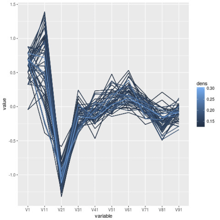
Figure 2: Million song subset, freqparcoord

As noted, the band is light and narrow. The lightness of the band — higher estimated density — merely signifies that songs in the dataset are disproportionately from later years. What is key, though, is the narrowness, which tells us that for the years 2004 onward, there was much less variation within each variable V2, V3 and so on than among the previous years. The use of Auto-Tune made things more uniform.

So, what happened around that time period? In 1997, a technology debuted called Auto-Tune, which performs corrections on a singer’s voice. Within a few years, virtually all song recordings were using Auto-Tune, resulting in the reduced variation seen in the figure. (The effect will be more clearly brought out with another technique, to be introduced below.)

Here is another example, using another well-known dataset, Turkish Student Instructor Evaluations, from the UCI Machine Learning Data Repository, Lichman (2013). Here $n=5820$ and $p=28$. (Five categorical variables have not been included.) The 28 ratings, on a 1-5 scale, included criteria such as “The course aims and objectives were clearly stated at the beginning of the period.” The result, plotted using standard parallel coordinates, is shown in Figure 3. This is not quite black-screen, but certainly lacking in any discernible pattern.

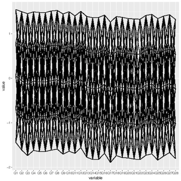
Figure 3: Turkish evaluations, ordinary parallel coordinates

This dataset would at first be considered an ideal candidate for using TFPC, but this actually presents a problem, since the data are discrete rather than continuous. In fact, the k-NN estimation process encounters a divide-by-0 problem, as a neighborhood often has volume 0. After applying R’s jitter() function (default value) and running freqparcoord, again with $F=50$, we have Figure 4.

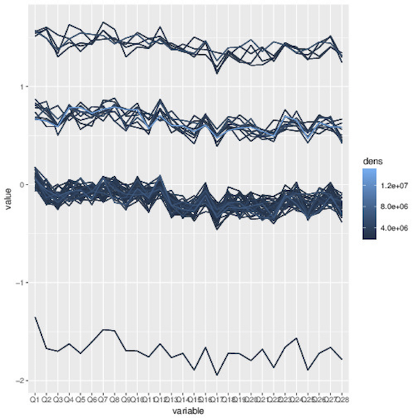
Figure 4: Turkish data with jitter, freqparcoord

Here the lines are rather flat, with little variation, even with the jitter. The implication is remarkable: Typically, a student gives identical responses to all 28 questions! Apparently the surveyors need not ask so many questions after all.

3 Discrete/Categorical Data

Most real datasets contain at least one categorical variable, typically many. TFPC methodology, aimed at illustrating continuous variables, does not work directly. Distance measures no longer make sense, as the data is non-ordinal.

Our freqparcoord package handles this by stacking separate plots atop each other. To illustrate this, consider the dataset mlb on U.S. major league baseball players, included in the package. Figure 5 shows the result for $F=5$, plotting height, weight and age, for positions Catcher, Infielder, Outfielder and Pitcher.

Again, the data is centered and scaled, with those parameters being determined by the data as a whole, not within-group. Look in particular at the weight variable: The catchers seem to be on the heavy side, confirming the popular image of “beefy” catchers.

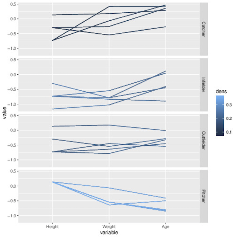
Figure 5: MLB data, freqparcoord

However, this approach is not feasible if a categorical variable has many levels. For example, in the mlb data, there are 30 teams, and certainly no room on a screen to stack 30 graphs. And this would be compounded when using the player position variable in addition to team, necessitating $30\times 4=120$ graphs. Converting to dummy variables would not be a solution either, with no room on the screen for the additional 119 columns.

The solution is to abandon using multivariate density as our measure of frequency. Instead, we make all variables discrete (including discretizing the continuous ones), and then simply measure frequency of a pattern by its count in the dataset.

This discrete/categorical case is the main focus of the present paper. It is implemented in our later package, cdparcoord, Matloff et al. (2017).

As our first example, consider the mlb data. We applied a discretize() function from the package, which (in default configuration) converts the numeric variables to nlevels equally-spaced quantiles. We then plotted the $F=50$ most common lines, and also performed a couple of mouse operations. The first mouse action allows one to drag a column to a new location, which we used to move the age variable to the far left, so that height and weight would be adjacent to player position. The second mouse operation involved brushing, implemented as clicking and dragging the Catcher node in the player position column up a bit, thus highlighting the catchers. (That portion of the Catcher axis then becomes highlighted in magenta, to indicate where the brushing was applied.) The result is shown in Figure 6. Note that the colored legend on the right shows frequencies.

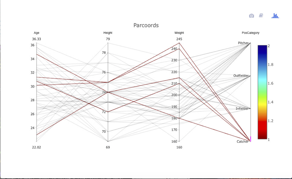
Figure 6: MLB data, cdparcoord

Here we see that the catchers not only tend to be somewhat heavier than average, but also somewhat shorter. The combination of those two traits, a “stocky” build, is again consistent with a general perception regarding catchers.

Another dataset included in the package is prgeng, involving programmers and engineers in the Silicon Valley area in the 2000 U.S. census. We removed those with salaries above $250,000, and plotted the top 150 lines, again brushing the female lines. The result is shown in Figure 7. Are the women underpaid?

It does appear that the women (sex code 2) tend to have lower wages (shown in the column wageinc). They do work in occupations that are somewhat lesser paid (100, 101, occ column) with Programmer titles, not Software Engineer (thus more likely in a bank, say, than a tech company), and not with Hardware Engineer titles (code 141). On the other hand, the males with the same job codes still seem to tend to have higher wages than their female peers. The important question of gender discrimination in Silicon Valley cannot be solved with such preliminary analysis and limited number of variables, but the example does show how TFPC may be used.

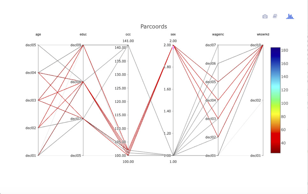
Figure 7: Programmer and engineer data, cdparcoord

Returning to the Turkish student evaluation data, with cdparcoord, with discrete / categorical TFPC there is now no need to add jitter, and with 25 lines we have Figure 8. Again, the most common lines are seen to be horizontal, meaning that students tend to give identical answers to the various questions. This plot does seem to indicate some nonconstancy within certain questions — e.g. an interesting drop from a 4 rating to a 2 from Question 11 to 13 — but again it appears that many more questions are being asked than is necessary.

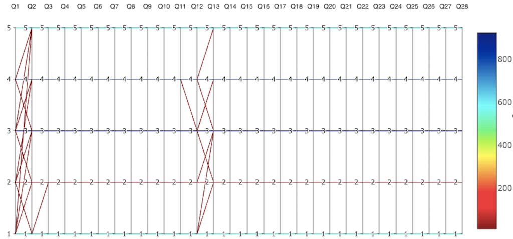
Figure 8: Turkish evaluation data, cdparcoord

It is important to be able to condition on more than one variable/value at a time. Consider for instance the Stanford WordBank vocabulary data, Wordbank (2016), involving very young children. The plot is shown in Figure 9. Here we have focused on girls of mothers having at least a college education, indicated by the magenta segments of two of the axes. Note that, at least at these very young ages, the relation between the mother’s education and the daughter’s vocabulary size is not as strong as one might guess a priori.

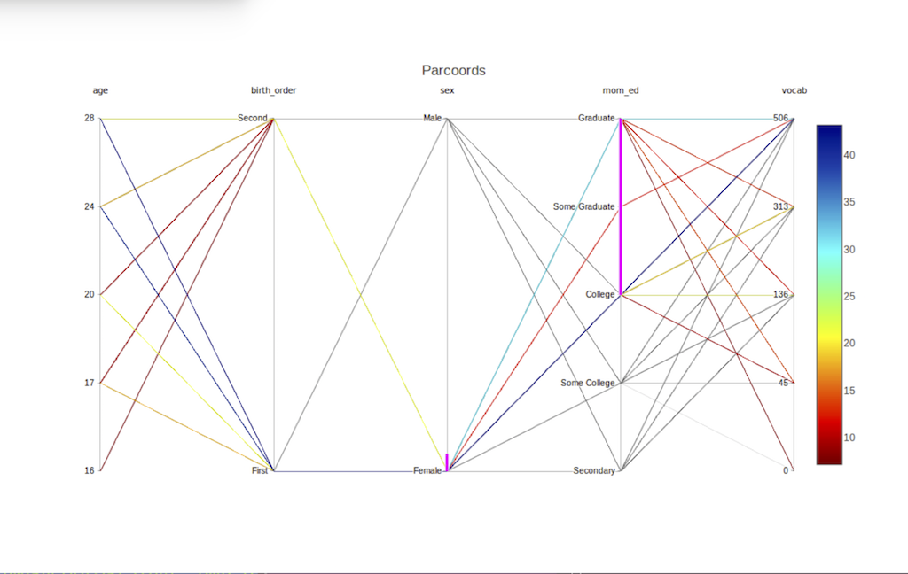
Figure 9: Stanford WordBank data, cdparcoord

4 Outlier Hunting

One advantage of frequency-based PCPs is that one can plot the least-frequent lines in order to search for possible outliers. Both the freqparcoord and cdparcoord packages allow for this, signified by the user specifying a negative number of lines to be plotted.

Here is an example, using the famous Pima diabetes dataset from the UCI repository. The call

discparcoord(pima,k=-25)

yields Figure 10. This is rather startling, as it shows that there are people in the dataset with 0 values for BP, BMI and insulin, a medical impossibility. Note too that at least one observation has more than one 0 (there are several), a fact we learn due to PCPs being multivariate methods. These observations should probably be removed from the data set.

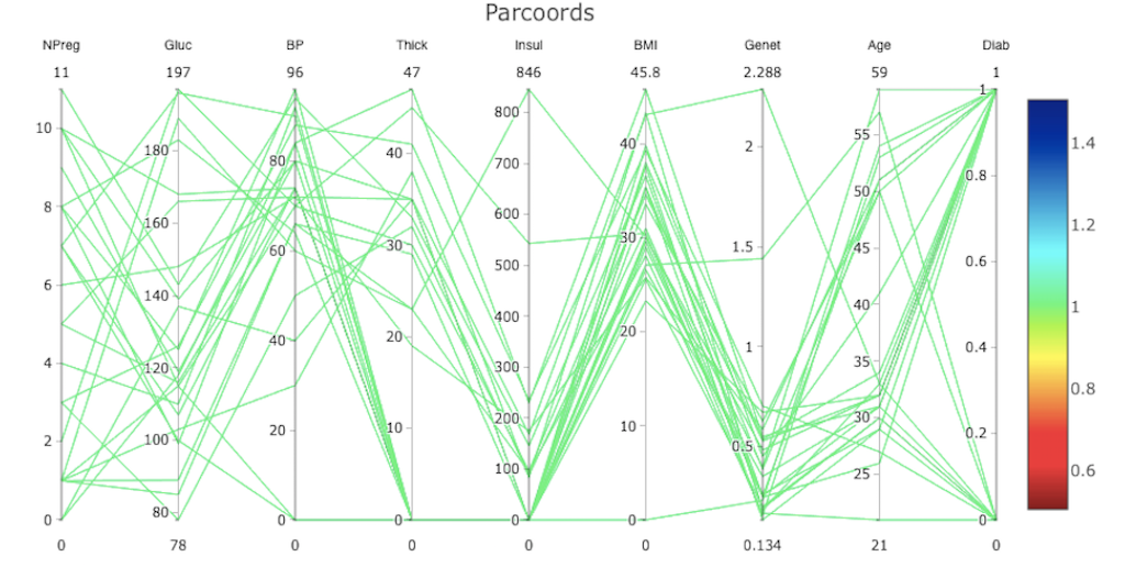
Figure 10: Diabetes data, outliers

The freqparcoord package allows one to optionally label lines with their index numbers within the dataset, making it easier to identify the outlier cases for possible action. (In cdparcoord, one has the option of saving a text file with all cases and their frequencies.) Here is an example using the mlb data, specifying 5 lines, in Figure 11.

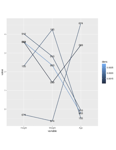
Figure 11: MLB data, outliers

Case 674 looks interesting, with extremely high age but somewhat low height and weight. Here is the record in the dataset:

        Name Team      Position Height Weight   Age  PosCategory
Julio_Franco  NYM First_Baseman     73    188 48.52  Infielder

Further investigation reveals that Franco later was still playing professional baseball at age 57.

5 Cluster Hunting

As noted earlier, TFPC may be viewed as similar to cluster analysis. However, since TFPC finds only the most frequent tuples, we run the risk of missing what amount to rare clusters.

In our freqparcoord package, this is handled via a locmax option. As the name implies, it specifies to display a tuple not according to whether it is among the overall highest frequencies but according to whether it has the highest frequency in a neighborhood.

In cdparcoord this approach is infeasible, due to the lack of a metric. However, one can force a known rare category to display by giving it extra weight in the tuple counting, via an accentuate argument.

6 Handling Missing Values

A problem with many real data sets is the prevalence of missing values, coded NA in R. Normally this would not be an issue with exploratory graphical methods such as parallel coordinates, which do not rely on precise point estimation. However, TFPC requires complete cases, and for large $p$ the chance of a particular case being complete may be quite low. This would result in a much smaller dataset to plot.

Take the Stanford WordBank vocabulary data mentioned earlier. There only 2741 of the 5498 cases are complete, with only $p=12$ variables. Datasets having a much larger $p$ could be even worse in this regard.

Here we propose several remedies. There is a vast literature on formal methods for handling missing values [Little and Rubin (2014)]. Here we use only the most restrictive of the major assumptions, Missing Completely at Random (MCAR), and then the somewhat less restrictive Missing at Random (MAR). We also propose a heuristic method.

It will be convenient to use conditional probability mass function notation $\pi$. For any (possibly incomplete) vector $X^{\prime}$ in our sample. let $X=(U,V)$ denote the true values of the components, where $U$ and $V$ denote the observed and unobserved components of the tuple; for simplicity we take $V$ to consist of a single component here. Let $M$ denote an indicator variable for the event that $V$ is missing. MCAR states that

$$\pi_{M~{}|~{}U,V}=\pi_{M}$$ (3)

i.e. missingness is entirely independent of the data.

MAR is a little more subtle:

$$\pi_{M~{}|~{}U,V}=\pi_{M~{}|~{}U}$$ (4)

i.e. missingness may be affected by the observed components but not the unobserved one. A commonly-offered example of MAR involves a mental health survey, and possible nonresponse. Let $U$ denote gender. Suppose male subjects are generally more reluctant to respond to a question on depression than are females, but suppose such reluctance in either gender is not affected by the degree of depression ($V$). Then MAR would hold.

In the following sections, we present outlines of three possible approaches.

6.1 Method of Moments Estimation

Here we assume MCAR. Let $X$ denote a randomly generated tuple from the population, including possibly unobserved components, and let $X^{\prime}$ denote the observed tuple, including NAs.

Let $\mathcal{T}$ denote the set of all possible tuples. Say for example we have $p=6$ variables, each taking on the values 1, 2 or 3. $\mathcal{T}$ then would be the 6-fold Cartesian product of the set $\{1,2,3\}$. For any $t\in\mathcal{T}$, let $p_{t}$ denote the population proportion for that tuple, i.e. $P(X=t)$.

Now let $\mathcal{T}^{\prime}$ denote the superset of $\mathcal{T}$ that includes tuples with NA values. In the above example, (2,2,1,3,NA,3) would be a member of this set, as would (NA,2,1,3,NA,3), and as would all of $\mathcal{T}$. For any $t^{\prime}\in\mathcal{T}^{\prime}$, let $M(t^{\prime})\subset\mathcal{T}$ be the collection of all tuples $t\in\mathcal{T}$ that become $t^{\prime}$ upon suitable replacement of components by NA. In ther words, $M(t^{\prime})$ is the set of intact tuples from which $t^{\prime}$ may have come. For any $t^{\prime}$, we will use $c(t^{\prime})$ to denote the count of NAs in $t^{\prime}$.

Finally, let $q$ denote the probability of an NA value. Under MCAR and the typical additional assumption that missingness is independent across components of a tuple, the probability that an observed tuple has NAs in $m$ specified components is $(1-q)^{p-m}q^{m}$.

The natural estimate of $q$ is the proportion of NAs in the $np$ tuple components in our data. We will take that estimate to be the true population value, but an alternating procedure along the lines of the EM algorithm could be used.

Then for any $t^{\prime}\in\mathcal{T}^{\prime}$, we have

$$P(X^{\prime}=t^{\prime})=(1-q)^{p-c(t^{\prime})}q^{c(t^{\prime})}\sum_{t\in M(t^{\prime})}p_{t}$$ (5)

Replace the left-hand side here by its direct sample estimate, the proportion of observed tuples that equal $t^{\prime}$, and continue to assume that $q$ is known. As we vary $t^{\prime}$, this gives us a system of linear equations in the $p_{t}$. Solving for the $p_{t}$ yields estimates for those quantities, $\widehat{p}_{t}$.

We can then determine the $F$ largest values of the $\widehat{p}_{t}$, and generate a TFPC plot that thus takes into account both the intact and partially-missing data.

6.2 An Update Method

Here we assume MAR, again for the sake of notational simplicity taking $V$ to consist of a single component. Missingness for that component will be denoted by $M$.

Using (4) we start with

$$\pi_{V|M,U} = \pi_{V,M,U}~{}/~{}\pi_{M,U}$$ (6)

$$= \pi_{M|U,V}\cdot\pi_{U,V}~{}/~{}\pi_{M,U}$$ (7)

$$= \pi_{M|U}\cdot\pi_{U,V}~{}/~{}\pi_{M,U}$$ (8)

All three expressions in the final equation can be estimated from our data: $\pi_{U,V}$ can be estimated from our complete-case data, while $\pi_{M|U}$ and $\pi_{M,U}$ can be estimated from our partially-observed data.

As a simple example, suppose $p=2$ and our data is

U	V
1	2
3	2
3	NA
3	2
3	1
2	2

Our tuple frequency table based on the intact cases is

U	V	Freq
1	2	1
3	2	2
3	1	1
2	2	1

Then we have the following estimates:

$$\widehat{P}(M=1~{}|~{}U=3)=1/4$$ (9)

$$\widehat{P}(U=3,V=1)=1/5$$ (10)

$$\widehat{P}(M=1,U=3)=1/6$$ (11)

From (8), we have

$$\widehat{P}(V=1~{}|~{}M=1,U=3)=(1/4)\cdot(1/5)~{}/~{}(1/6)=3/10$$ (12)

Similarly, $\widehat{P}(V=2~{}|~{}M=1,U=3)=2/5$. and thus $\widehat{P}(V=1~{}|~{}M=1,U=3)=1/10$.

We can thus “update” our tuple frequency table, counting the (3,NA) tuple 3/10 for (3,1), 2/5 for (3,2) and 1/10 for (3,3):

U	V	Freq
1	2	1
3	2	2.6
3	1	1.3
2	2	1
3	3	0.1

In that manner, we can proceed iteratively, with one update for each non-intact observation. At any stage, we could use the new frequency table in calculating the quantities in (4).

The final frequency table would then be used in forming the parallel coordinates plot.

6.3 A Heuristic Approach

The MCAR and MAR models are of course restrictive. For instance, MCAR treats missingness as being independent across variables, a condition that may not hold in some data sets.

In the Stanford WordBank data mentioned earlier, for instance, about 13.5% of the data values are NAs. Under MCAR, the probability of a row being complete would then be $(1-0.135)^{13}$, about 0.152. Yet the actual proportion is $2741/5498$, about 0.499. In other words, the NA values tend to clump.

Again, the missing-values field is vast, and the methods are assumption-laden. Furthermore, one must keep in mind the implications of the fact that the cases having missing values may be systemically different from the others. Nevertheless, a simple heuristic may be of value. One is included in our package cdparcoord, as a tuning parameter NAexp, which we now describe.

For concreteness, consider this simple example, with $p=6$ and with each variable taking on the integers between 1 and 3. Suppose we have the observation (2,2,1,3,NA,3). It could have been (2,2,1,3,1,3), (2,2,1,3,2,3) or (2,2,1,3,3,3). Intuitively, it would seem wrong to ignore the information that this observation mostly matches these three tuples.

One way to use such information would be to give $(1/3)\times(5/6)=5/18$ credit for each of the three possibilities. In our package cdparcoord, there is a tuning parameter NAexp that allows the user to choose how much to count such partial matches. In the above example, the 5/6 figure would be taken to the NAexp power.

7 Why Not Just Subsample?

As noted earlier, one approach to the BSP is to draw a random subsample of size $N$ from the data, consisting of say, hundreds or thousands of data points, and then form a PCP from the subsample. However, the loss of information due to subsampling may obscure important trends or create spurious ones especially if $p/N$ is large, essentially the multiple inference problem. Important outliers may also be missed.

To compare the subsampling and TFPC approaches, consider the diamonds data, bundled with the ggplot2 package. We took a subsample of size 2500 (out of almost 54000), and ran an ordinary PCP on the subsample. We then ran cdparcoord on the the full data set, but with the $F=2500$ most-frequent lines.

The results are shown in Figures 12 and 13. Looking at the Premium grade, for instance, there is a clear trend in the TFPC version, seen in the blue line. This is much harder to see in the subsampled, standard PCP.

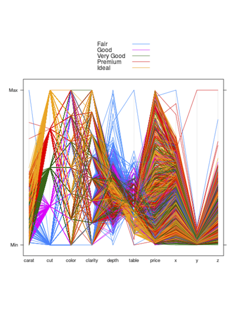
Figure 12: Diamond data, PCP on subsample, $N=2500$

Figure 13: Diamond data, cdparcoord, $F=2500$

8 Computational Issues

Though the tabulation of tuple frequencies could easily be parallelized, there would seem to be no need even for fairly large datasets. For instance, simulated data with $n=1000000$ and $p=150$ and 10 values for each variable took only about 20 seconds to process on a low-end laptop. In any event, parallel computation of frequency counts is offered in cdparcoord.

Implementation of the NA models proposed above could be more intensive in both computational time and memory space. Parallelization of the solution of linear systems brings only limited speedup [Matloff (2015)], and again, memory space may be an issue.

9 Discussion and Conclusions

There has been much work on visualization methods for the categorical data case, such as Pilhöfer and Unwin (2013) and Hoffman and Vendettuoli (2016). All of them have settings in which they work well. In this paper, we add TFPC as another possible choice for those interested in data visualization.

For advanced usage, there is elegant geometric theory that can aid in acquiring insight from the data [Inselberg (2009)]. For example, say two variables that are adjacent in a parallel coordinates plot have a strong negative correlation. Then the lines between these two columns will tend to approximately converge at a common point between the columns. However, there is no insight to be gained if one has the black screen problem, and TFPC is one solution to the latter.

As pointed out in Murrell (2016), techniques for categorical data tend to be lesser known than continuous-variable methods, even though a number of useful methods have been developed. There are for instance as parallel sets, Kosara et al. (2006) and mosaic plots, Unwin et al. (2007). However, though these are highly effective for a small number of variables, there typically is not enough room on the screen, or in the viewer’s perceptive abilities, to display larger numbers of variables.

Thus we believe parallel coordinates methods, including TFPC, holds great promise. But even putting the “black screen problem” aside, users cannot expect to necessarily have quick, automatic “Eureka!” responses when viewing such a plot. These issues were described well in Ben Shneiderman’s Forward to Inselberg (2009). While he speaks of “the cleverness and power” of the parallel coordinates approach, Shneiderman admits to “struggling” with interpreting some of these plots.

The benefits of the parallel coordinates approach do require patience. In addition, as an exploratory tool, the analyst may find it useful to generate several plots of the same data, changing for example the number of lines plotted, the order of the columns, the use of brushing and so on.

But as the examples presented here show, the TFPC approach can yield excellent insight, including in datasets having many categorical variables. The “black screen problem” is handled in a simple, natural manner.

SUPPLEMENTARY MATERIAL

Code listings:

For Figure 1:

# had earlier generated and saved a 50K subsample from
# https://archive.ics.uci.edu/ml/datasets/YearPredictionMSD
library(data.table)
ms <-
   fread(’~/DataSets/MillionSong/FiftyKSongs.csv’,header=TRUE)
ms <- as.data.frame(ms)
ms <- ms[,seq(1,91,10)]
ggparcoord(ms,1:10)

For Figure 2:

library(cdparcoord)  # brings in freqparcoord auto
# ms from above
freqparcoord(ms,m=50)

For Figure 3:

turk <-
   read.csv(’~/DataSets/TurkEvals/turkiye-student-evaluation.csv’,
      header=TRUE)
turk <- turk[,-(1:5)]
ggparcoord(turk,m=50)

For Figure 4:

# turk as above
turkj <- turk
for (i in 1:28) turkj[,i] <- jitter(turk[,i])
freqparcoord(turkj,m=50)

For Figure 5:

data(mlb)
freqparcoord(mlb,5,4:6,7)

For Figure 6:

# mlb as above
discparcoord(mlb[,4:7],k=50)
# click and drag Age to far left
# click Catcher, see +, then drag up a bit

For Figure 7:

data(prgeng)
pe <- prgeng[,c(1,3,5,7:9)]
pe1 <- pe
pe25 <- pe1[pe1$wageinc < 250000,]
pe25 <- makeFactor(pe25,c(’educ’,’occ’,’sex’))
pe25disc <- discretize(pe25,nlevels=5)
discparcoord(pe25disc,k=150)

For Figure 8:

# turk as above (but no jitter added)
trk <- turk
# convert ints to factors, so have e.g. 2 not 2.00
for (i in 1:28) trk[,i] <- as.factor(turk[,i])
discparcoord(trk,k=25)

For Figure 9:

wb <- wb[,c(2,5,7,8,10)]
wb <- discretize(wb,nlevels=5)
wb <- reOrder(wb,’mom_ed’,
   c(’Secondary’,’Some College’,’College’,’Some Graduate’,’Graduate’))
discparcoord(wb,k=100)

For Figure 10:

pima <-
   read.csv(’~/Research/DataSets/Pima/pima-indians-diabetes.data’,
      header=TRUE)
discparcoord(pima,k=-25)

For Figure 11:

# mlb as above
freqparcoord(mlb,-5,4:6,plotidxs=TRUE)

For Figure 12:

library(lattice)
ds <- diamonds[sample(nrow(diamonds), 2500),]
parallelplot(~ds, group = cut, data = ds, horizontal.axis = FALSE,
             auto.key = TRUE)

For Figure 13:

dd <- discretize(diamonds,nlevels=4)
discparcoord(dd,k=2500)

References

- Bertin-Mahieux et al. (2011) Bertin-Mahieux, T., Ellis, D. P., Whitman, B., and Lamere, P. (2011). The million song dataset. In Proceedings of the 12th International Conference on Music Information Retrieval (ISMIR 2011).
- Bühlmann et al. (2016) Bühlmann, P., Drineas, P., Kane, M., and van der Laan, M. (2016). Handbook of Big Data. Chapman & Hall/CRC Handbooks of Modern Statistical Methods. CRC Press.
- Hoffman and Vendettuoli (2016) Hoffman, H. and Vendettuoli, M. (2016). ggparallel: Variations of parallel coordinate plots for categorical data. https://cran.r-project.org/web/packages/ggparallel/index.html.
- Inselberg (2009) Inselberg, A. (2009). Parallel Coordinates: Visual Multidimensional Geometry and Its Applications. Advanced series in agricultural sciences. Springer New York.
- Kosara et al. (2006) Kosara, R., Bendix, F., and Hauser, H. (2006). Parallel sets: Interactive exploration and visual analysis of categorical data. Visualization and Computer Graphics, IEEE Transactions on, 12(4), 558–568.
- Lichman (2013) Lichman, M. (2013). UCI machine learning repository. http://archive.ics.uci.edu/ml.
- Little and Rubin (2014) Little, R. and Rubin, D. (2014). Statistical Analysis with Missing Data. Wiley Series in Probability and Statistics. Wiley.
- Matloff (2015) Matloff, N. (2015). Parallel Computing for Data Science: With Examples in R, C++ and CUDA. Chapman & Hall/CRC The R Series. CRC Press.
- Matloff and Xie (2013a) Matloff, N. and Xie, Y. (2013a). freqparcoord: Novel methods for parallel coordinates. https://cran.r-project.org/web/packages/freqparcoord/index.html.
- Matloff and Xie (2013b) Matloff, N. and Xie, Y. (2013b). A new look at the parallel coordinates method for large data sets. In JSM 2013.
- Matloff et al. (2017) Matloff, N., Yang, V., and Nguyen, H. (2017). Top frequency-based parallel coordinates. https://github.com/matloff/cdparcoord.
- Murrell (2016) Murrell, P. (2016). R Graphics, Second Edition. Chapman & Hall/CRC The R Series. CRC Press.
- Pilhöfer and Unwin (2013) Pilhöfer, A. and Unwin, A. (2013). New approaches in visualization of categorical data: R package extracat. Journal of Statistical Software, Articles, 53(7), 1–25.
- Unwin et al. (2007) Unwin, A., Theus, M., and Hofmann, H. (2007). Graphics of Large Datasets: Visualizing a Million. Statistics and Computing. Springer New York.
- Wegman (1990) Wegman, E. J. (1990). Hyperdimensional Data Analysis Using Parallel Coordinates. Journal of the American Statistical Association, 85, 664–675.
- Wordbank (2016) Wordbank (2016). Wordbank: an open database of children’s vocabulary development. http://wordbank.stanford.edu/.