Distortion Minimization for Relay Assisted Wireless Multicast

Abstract

The paper studies the scenario of wireless multicast with a single transmitter and a relay that deliver scalable source symbols to the receivers in a decode-and-forward (DF) fashion. With the end-to-end mean square error distortion (EED) as performance metric, we firstly derive the EED expression for the $L$-resolution scalable source symbol for any receiver. An optimization problem in minimizing the weighted EED is then formulated for finding the power allocations for all resolution layers at the transmitter and the relay. Due to nonlinearity of the formulations, we solve the formulated optimization problems using a generalized programming algorithm for obtaining good sub-optimal solutions. Case studies are conducted to verify the proposed formulations and solution approaches. The results demonstrate the advantages of the proposed strategies in the relay-assisted wireless networks for scalable source multicast.

I Introduction

Wireless communication suffers from multipath fading and the time-varying characteristic, which causes distortion to the delivered information. To resolve this problem, joint source-channel coding (JSCC) is shown promising in practical wireless communication systems. JSCC pairs scalable source coding (SSC) and superposition channel coding (SPC) by mapping the source symbols to multiple successively refined channel symbols. The source from a common source coding block is scalably encoded into several resolutions/layers and then mapped into successively refined source symbols at the transmitter. These source symbols are then mapped into channel symbols and superimposed into one JSCC symbol under SPC for transmission. Employing successive interference cancelation (SIC), each receiver can then recover up to a specific layer of JSCC symbols with respect to its channel quality [1]-[4].

In [1], the expected distortion of transmission of a Gaussian source over a slow fading channel with only a finite number of fading states is investigated. In [2], the problem of transmitting a Gaussian source on a slowly fading Gaussian channel is studied, subject to the mean squared error distortion measure. [3] finds new tight finite block-length bounds for the best achievable lossy joint source-channel code rate. In [4], reliable transmission of a discrete memoryless source to multiple destinations over a relay network is considered, where the relays and the destinations all have access to side information correlated with the underlying source signal.

Numerous efforts have been claimed on multi-resolution SPC over wireless transmissions [5]-[11]. In [5], bit allocation for a joint source/channel video codec over static channels is studied, and the expected distortion is minimized through the distribution of the available bits among the subbands. In [6], the optimal selection of the JSCC rates through all layers over Rayleigh fading channels is presented in terms of the overall distortion. The energy efficiency of various JSCC problems is studied in [7]. In addition, the JSCC problem of using hybrid digital analog codes in transmitting a Gaussian source over a Gaussian channel is studied in [8]. [9] presents a distributed JSCC system for relay systems exploiting spatial and temporal correlations. In [10], an optimal noise channel quantization with random index assignment in a single-layer tandem source channel coding system with one-level resolution is investigated. In [11], the SPC transmission for scalable sources of only two information layers over relay channels is investigated, and the performance improvement is evaluated. [12] presents an optimal JSCC broadcasting scheme by providing different QoS metrics for heterogeneous users in the network by employing fountain codes. In [13], a JSCC model over the MIMO broadcast channel is presented to minimize the sum mean square error distortion, where the perfect channel state information (CSI) is assumed to be available at the transmitter and at the receivers. [14] investigates the average throughput and distortion of a multi-relay aided unicast system with two-layer resolution sources, where the direct link is assumed to be unavailable.

It is clear that most existing works on JSCC have focused on theoretical performance such as channel capacity, outage probability and distortion exponent, which may nonetheless fail to faithfully reflect the end-to-end (E2E) service quality in terms of symbol error rates. Further, those theoretical performance metrics are only suitable as metrics under high signal-to-noise ratio (SNR) regime, which however are not suitable under low SNR regime with high channel error probabilities.

In this paper, we are committed in a new research initiative on the resource allocation problems for multicasting of JSCC symbols, where the transmit power of each resolution layer at both transmitter and relay are jointly determined. The aim is to minimize the weighted averaged EED of all users.

The contributions of this work are summarized as follows,

• introduce a general framework of JSCC transmission for successively refined information source with an arbitrary number of layers over relay networks.

• formulate an optimization problem for jointly determining the power assigned to all resolution layers at both the source node and relay for the weighted averaged EED of all users.

• develop a generalized programming algorithm that employs a Lagrangian dual method to solve the formulated problems to obtain a good sub-optimal solution.

The rest of this paper is organized as follows. Section II presents the system model. Section III provides the EED model. Section IV presents the formulated optimization problems under various target functions, along with the proposed generalized programming algorithm to obtain good sub-optimal solutions. Simulation results are presented in Section V and the paper is concluded in Section VI.

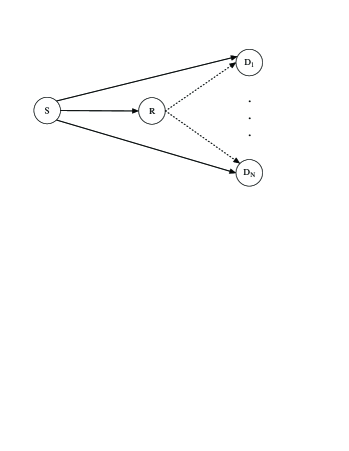
Figure 1: The relayed multicast network considered in the system model, where the solid line denotes the transmission in the first time slot and the dash line denotes transmission in the second slot.

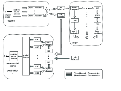
Figure 2: The encoding/decoding structure of scalably encoded sources with successive refinement of a general $L$-resolution multicast, where the received signals from the direct link and the relay links are decoded separately at each destination. At the scalable source encoder at source node, the information is encoded at different resolutions/layers with the associated CRC part attached to the constructed message in help of decoding at the CRC module of the relay and destination nodes. The received messages at each node are then fed into the cyclic redundance codes (CRC) module for error detection and then processed at the symbol detector for information reconstruction. It is also noted that each time slot is equally divided into two time subslots, where the first subslot is used for source transmission and the second subslot is used for relay transmission, respectively.

TABLE I: The notion table of the parameters in this work

$N$	the number of receivers/destination nodes
$L$	the number of refined layers for a source symbol
$\mathtt{P}_{i}$	the average transmit power constraint at node $i$
$P_{i}$	the transmit power at node $i$
$\beta_{l}^{(i)}$	the ratio of power assigned to layer $l$ at node $i$
$\boldsymbol{\beta^{(i)}}$	the power allocation vector of node $i$
$h_{ij}$	the channel gain of link $i$-$j$
$p_{err,d_{n}}^{(l)}$	the E2E SER of up to layer $l$ at the end of the second slot at receiver $d_{n}$
${\tt p}_{d_{n}}^{(l)}$	the realization probability of only to layer $l$ information successfully decoded at $d_{n}$
$N_{0}/2$	the two-sided power spectral density of the additive white Gaussian noise
$EED_{d_{n}}$	the end-to-end distortion at $d_{n}$ given channel realizations and power allocations.

II System Description

As shown in Fig. 1, a relay-aided multicast network consists of one source node, one relay and $N$ destination nodes. The general encoding/decoding structure of a JSCC system is shown in Fig. 2. The discrete-time, real-valued continuous Gaussian information source at the source node is scalably encoded and mapped into successively refined symbols of $L$ layers, and is broadcasted via both the direct ($s\rightarrow d_{n}$, $n=1,\ldots,N$) links and the relayed ($s\rightarrow r$ and $r\rightarrow d_{n}$) links to enable the multi-resolution information reconstruction at the destination nodes. The $L$ layers mapped by the scalable information source are correspondingly denoted by the base layer, the first enhancement layer, $\ldots$, and the ($L-1$)th enhancement layer, respectively. Among them, the base layer alone provides the lowest resolution reconstruction. By adding more enhancement layers incorporating with the base layer gradually improves the resolution reconstruction to a higher level, while adding the base layer and all $L-1$ enhancement layers altogether provide the highest resolution reconstruction. Before transmission, each source symbol corresponding to each layer is mapped into one or a set of channel symbols and the channel symbols of all the symbols of $L$ layers are further superimposed under SPC. For reference, a typical example showing the procedure of SPC constellation of the symbols of each layer for a two-layer case is shown in Fig. 3. Further, for readability, the definitions of some parameters used in this work are listed in Table. I.

Let the average transmit power constraint at the source node and the relay node be denoted by $\mathtt{P}_{s}$ and $\mathtt{P}_{r}$. In addition, the actual transmit power at source and relay are denoted by $P_{s}$ and $P_{r}$, respectively. For the power assigned to each layer, it is assumed that $\beta_{1}^{(i)}P_{i}$ ($i=s,r$) is allocated to the base layer at node $i$, and $\beta_{l}^{(i)}P_{i}$ ($l=2,\ldots,L$) is allocated to the $(l-1)$th enhancement layer, where $\beta_{L}^{(i)}=1-\sum_{l=1}^{L-1}\beta_{l}^{(i)}\geq 0$ is for the $(L-1)$th enhancement layer and it is physically required that $\beta_{l}^{(i)}\geq 0$ ($\forall i,l$). The power allocation vector at node $i$ is also referred to as $\boldsymbol{\beta^{(i)}}=\{\beta_{l}^{(i)}|l=1,\cdots,L\}$ for simplicity. Note that both the vector representation and the scalar representation of the power assignment parameter will be used interchangeably in the following analysis.

The general encoding/decoding structure of a JSCC system is shown in Fig. 2. In the first time subslot, the source node broadcasts the JSCC symbols to the relay node and all the receivers. In the second time subslot, the source node keeps silent and the relay node broadcasts its decoded and re-encoded SPC symbols to all destination nodes, possibly with a different power allocation ($\beta_{l}^{(r)}$) for different layer symbols.

When a JSCC symbol is received (either at the relay or the destination), it is firstly decoded as if it just contains the base layer symbol while taking all the other layer energy as interference. Once the base layer is correctly obtained, it is subtracted from the JSCC symbol, resulting in a new JSCC symbol, which is in turn decoded as if it is just for the first enhancement layer symbol while taking all the other layer energy as interference. Such an iterative and successive decoding process, also known as successive interference cancelation (SIC), proceeds up to the $L$-th layer, which is defined according to the instantaneous channel quality perceived at the receiver.

Further, it should be noted that, at the end of the first time subslot, the received messages of each layer at relay from the source transmitter is fed into the cyclic redundancy code (CRC) module for error detection and messages of the successfully decoded layers are re-encoded and superimposed for transmission to the destinations at the second subslot. It is also noted that CRC is performed at the layer level for higher system performance.

At the end of the second time subslot, the received information from both the direct and relay links, respectively, is fed into the cyclic redundancy code (CRC) module for error detection and then processed by the symbol selector to determine the reconstructed bits of the channel use.

With the above mentioned SIC decoding process, a number of $L+1$ events with different probabilities can be defined according to the instantaneous channel capacity, where the first event denotes the loss of all information layers, the second event denotes only the base layer is successfully obtained, and the $l$th ($2<l\leq L+1$) event denotes that the base layer and enhancement layers $1,\ldots,l-2$ are successfully obtained.

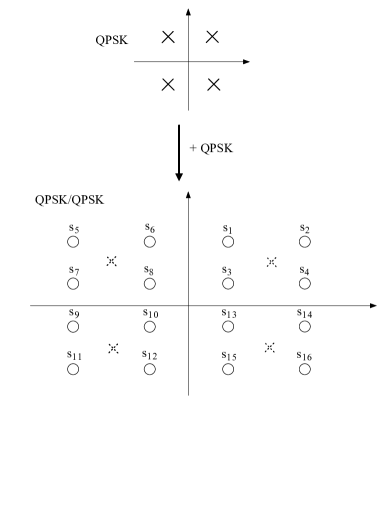
Figure 3: The procedure of SPC constellation with two layers using QPSK and QPSK signals as the base layer and the enhancement layer, respectively.

III System Model

In this section, we provide an end-to-end distortion (EED) model for an $L$-layer JSCC relay-aided multicast network.

III-A Channel Model

Consider a Nakagami-$\rho$ fading channel where $m$ is the Nakagami parameter representing the severity of the channel fading fluctuations, which degrades to the special Rayleigh fading model with $\rho=1$. Further, it is assumed that he channel gains of all links remain unchanged within one slot (where one slot consists of two equally divided sub-slots for the direct transmission and relayed transmission, respectively) and are independent from each other in different slots for different links. In addition, it is assumed that each transmitter only has the statistics of the channel state information (CSI).

The probability density function (pdf) $f_{h}(h_{ij})$ and the cumulative density function (cdf) $F_{h}(h_{ij})$ of the channel power gain over link $i\rightarrow j$ ($i=s,r$ and $j=r,d_{1},\ldots,d_{N}$), are given by,

$$f_{h}(h_{ij})=(\frac{\rho}{\bar{h}_{ij}})^{\rho}\frac{h_{ij}^{\rho-1}}{\Gamma(\rho)}\exp(-\frac{\rho}{\bar{h}_{ij}}h_{ij})$$ (1)

$$F_{h}(h_{ij})=\frac{\gamma(\rho,\frac{\rho}{\bar{h}_{ij}}h_{ij})}{\Gamma(\rho)}=\frac{1-\Gamma(\rho,\frac{\rho}{\bar{h}_{ij}}h_{ij})}{\Gamma(\rho)}$$ (2)

where $\gamma(\cdot,\cdot)$ and $\Gamma(\cdot,\cdot)$ are the lower and upper incomplete Gamma functions, respectively. $h_{ij}$ and $\bar{h}_{ij}$ are the instantaneous channel power gain and its average value, respectively. In addition, we have $\bar{h}_{ij}=1/d_{ij}^{\alpha}$ accounting for the large-scale fading, where $\alpha$ is the pass-loss exponent and $d_{ij}$ is the distance between node $i$ and $j$. Hence the average receiver-side power level is $\bar{\gamma}_{ij}=P_{i}\bar{h}_{ij}$ where $P_{i}$ ($i=s,r$) is the transmit power at the transmitter $i$. In addition, we denote $N_{0}/2$ as the two-sided power spectral density of the additive white Gaussian noise (AWGN).

In the following, with the assumption that the power allocated to each layer is specified and the channel gains are known, the E2E SER of up to layer $l$ at the end of the second slot at $d_{n}$, denoted by $p_{err,d_{n}}^{(l)}$, is hence given by,

$$p_{err,d_{n}}^{(l)}= p_{sd_{n}}^{(l)}\left(1-\left(1-p_{sr}^{(l)}\right)\left(1-p_{rd_{n}}^{(l)}\right)\right),$$ (3)

where $p_{ij}^{(l)}$ is the SER of the $l$th layer infomation over link $i$-$j$. Note that the product in (3) follows from the independence of transmission of different links and the terms in the outer bracket denotes the SER probability that at least one of the $s\rightarrow r$ and $r\rightarrow d_{n}$ links fails to provide decodable version of up to layer $l$ in relayed transmission given the realized channels. For reference, the detailed derivation of E2E SER of (3) as well as that of $p_{ij}^{(l)}$ is presented in Appendix C and are omitted here for brevity.

III-B Proposed EED model

With the allocated power for each layer at the source and relay as well as the instantaneous channel qualities over link $i\rightarrow j$, the reconstruction quality ($RQ$) at receiver $j$ for this transmission can be divided into $L+1$ categories (referring to decoding quality of the $L$ layer symbol), namely ${\tt L}_{ij}^{(0)}$, ${\tt L}_{ij}^{(1)}$, $\ldots$ and ${\tt L}_{ij}^{(L)}$, where ${\tt L}_{ij}^{(L)}$ represents the case that all layer information are corrected decoded and the symbol is perfectly reconstructed at node $j$. ${\tt L}_{ij}^{(0)}$ defines the case that all layer information is lost in this transmission over link $i\rightarrow j$. In addition, ${\tt L}_{ij}^{(l)}$ ($0<l\leq L$) indicates the case that only the lower $l$ layers are decoded for this transmission, including the base layer and the $l-1$ lower enhancement layers.

Taking both the direct and relay links for a specific destination node, i.e., $d_{n}$ into account, ${\tt L}_{d_{n}}^{(l)}$ is defined as the category in which only $l$ lower layers can be successfully decoded at $d_{n}$. Clearly, in category ${\tt L}_{d_{n}}^{(0)}$, the $s\rightarrow d_{n}$ link and at least one of $s\rightarrow r$ link and $r\rightarrow d_{n}$ link are not able to support even the delivery of the base layer information and the source information is totally lost at destination node $d_{n}$. In category ${\tt L}_{d_{n}}^{(l)}$ ($0<l<L$), only the base layer and up to the $(l-1)$th enhancement layer can be successfully obtained at the destination node $d_{n}$ through either the direct or the relayed links. In category ${\tt L}_{d_{n}}^{(L)}$, all layered source symbols are successfully reconstructed at the destination node $d_{n}$. Given the channel realizations, the associated realization probabilities of such events at destination node $d_{n}$ are therefore given by,

$${\tt p}_{d_{n}}^{(0)}=p_{err,d_{n}}^{(1)}$$ (4)

$${\tt p}_{d_{n}}^{(l)}=p_{err,d_{n}}^{(l+1)}-p_{err,d_{n}}^{(l)},\quad l=1,\ldots,L-1$$ (5)

$${\tt p}_{d_{n}}^{(L)}=1-p_{err,d_{n}}^{(L)}$$ (6)

where in (5) the difference between the E2E SER of up to layer $l+1$ and $l$ is the realization probability of successfully decoding only up to layer $l$.

III-C EED Evaluation

In [10] and [11], the EED expressions for one-level and two-level resolution cases are derived, respectively. The non-asymptotic EED expression for the realized channel gains of all links under generally $L$ layers can be derived in a similar way, which is given in Appendix C. The associated EED expression given the instantaneous channel gains that can reconstruct the information source at destination node $d_{n}$, denoted by $EED_{d_{n}}$, can hence be given by

$$EED_{d_{n}}(h_{sd_{n}},h_{sr},h_{rd_{n}})$$

$$= \sum_{l=1}^{L}D_{Q_{l}}{\tt p}_{d_{n}}^{(l)}+\sigma^{2}{\tt p}_{d_{n}}^{(0)}$$

$$= D_{{Q}_{L}}\left(1-p_{err,d_{n}}^{(L)}\right)+\sum_{l=1}^{L-1}D_{Q_{l}}\left(p_{err,d_{n}}^{(l+1)}-p_{err,d_{n}}^{(l)}\right)$$

$$\,\,\,+\sigma^{2}p_{err,d_{n}}^{(1)}$$ (7)

where $\sigma^{2}$ in this case is the variance of the Gaussian source signal and $D_{Q_{l}}$ denotes the quantization distortion in the reconstruction of the scalable source up to layer $l$.

By considering a real-valued Gaussian source with unit-variance, its distortion exponent is denoted by the R-D function $D_{RQ}=2^{-2R}$, where $R$ is the number of bits of each symbol. Therefore, combining it with (7) together leads to (8) as follows,

$$EED_{d_{n}}(h_{sd_{n}},h_{sr},h_{rd_{n}})$$

$$= \sum_{l=1}^{L}2^{-2\sum_{j=1}^{l}R_{j}}{\tt p}_{d_{n}}^{(l)}+\sigma^{2}{\tt p}_{d_{n}}^{(0)}$$ (8)

$$= 2^{-2\sum_{j=1}^{L}R_{j}}\left(1-p_{err,d_{n}}^{(L)}\right)$$

$$\,\,+\sum_{l=1}^{L-1}2^{-2\sum_{j=1}^{l}R_{j}}\left(p_{err,d_{n}}^{(l+1)}-p_{err,d_{n}}^{(l)}\right)+\sigma^{2}{\tt p}_{d_{n}}^{(0)}$$

where $R_{l}$ is the number of bits allocated to the $i$th layer per symbol under the $L$-layer JSCC architecture. For instance, if the base layer employs BPSK, we have $R_{1}=1$ bit for each symbol, i.e., the base layer contains $1$ bit information per symbol superimposed with other upper layer symbols.

By averaging the EED expressions over the channel realizations of all associated links (S-R,S-$d_{n}$,R-$d_{n}$), the expected EED at destination node $d_{n}$ is given by,

$$\overline{EED}_{d_{n}}= \iiint\limits_{h_{sd_{n}},h_{sr},h_{rd_{n}}}\,EED_{d_{n}}(h_{sd_{n}},h_{sr},h_{rd_{n}})f_{h}(h_{sd_{n}})$$

$$\,\,f_{h}(h_{rd_{n}})f_{h}(h_{sr})\,\mathrm{d}h_{sd_{n}}\,\mathrm{d}h_{sr}\,\mathrm{d}h_{rd_{n}}$$ (9)

Interestingly, an inequality can be derived from the EED expressions in (8) and (9) as follows.

$$0<2^{-2\sum_{j=1}^{L}R_{j}}\leq EED_{d_{n}}\leq\sigma^{2},\quad n=1,\cdots,N$$ (10)

$$0<2^{-2\sum_{j=1}^{L}R_{j}}\leq\overline{EED}_{d_{n}}\leq\sigma^{2},\quad n=1,\cdots,N$$ (11)

where the lower bound holds true when all $L$ layers are successfully decoded and the upper bound holds true when all $L$ layers are lost.

IV Formulation for EED Minimization

We take the target function as for minimizing the weighted sum of EEDs of all source-destination pairs. The optimization problem, termed as Popt, is then formulated as follows.

$$\min_{\boldsymbol{\beta^{(i)}},P_{i}}\quad\sum_{n=1}^{N}c_{n}\overline{EED}_{d_{n}}$$ (12)

subject to

$$\boldsymbol{\beta^{(i)}}\geq 0,\quad i=s,r$$ (13)

$$\mathbf{1}^{T}\boldsymbol{\beta^{(i)}}\leq 1,\quad i=s,r$$ (14)

$$0\leq P_{i}\leq\mathtt{P}_{i},\quad i=s,r$$ (15)

where in (12) the averaged EED of each user is from (9) by taking the expected value of EED in (8) over all realizations of the associated links. $c_{n}$ is the predefined weight for the $n$th user and we have $0\leq c_{n}\leq 1$ and $\sum c_{n}=1$. (13) gives the natural non-negative property of the feasible power allocation vectors and (14) serves as the normalization constraint for the power allocation vectors. (15) gives the average transmit power constraint, where $P_{i}$ is the transmit power at node $i$ ($i=s,r$) and should be constrained. It can be readily found that the optimal solution is achieved when $P_{i}=\mathtt{P}_{i}$ and we can simply replace $P_{i}$ with $\mathtt{P}_{i}$ under a numerical method.

Note that Popt is a non-convex optimization problem and the global optimal solution is difficult to be solved. Henceforth, the Lagrangian dual method is employed to find the solution to the dual problem of Popt, which serves as a very good lower bound to Popt.

Let $\nu^{(i)}$ ($i=s,r$) be the dual variables of Popt associated with the physical normalization constraint of the power allocation vectors in (14), respectively. The Lagrangian of problem P1 can then be expressed as,

$$L^{\bf P1}(\boldsymbol{\beta^{(i)}},\nu^{(i)})=\sum_{n=1}^{N}c_{n}\overline{EED}_{d_{n}}+\sum_{i=s,r}\nu^{(i)}\left(\mathbf{1}^{T}\boldsymbol{\beta^{(i)}}-1\right)$$ (16)

subject to $\boldsymbol{\beta^{(i)}}>\boldsymbol{0}$. The associated Lagrangian dual function of $L^{\bf P1}(\boldsymbol{\beta^{(i)}},\nu^{(i)})$ in (16) is defined as,

$$g^{\bf P1}(\nu^{(i)}) =\min_{\boldsymbol{\beta^{(i)}}>\boldsymbol{0}}\quad L^{\bf P1}(\boldsymbol{\beta^{(i)}},\nu^{(i)}).$$ (17)

$$=\min_{\boldsymbol{\beta^{(i)}}>\boldsymbol{0}}\quad\sum_{n=1}^{N}c_{n}\overline{EED}_{d_{n}}+\sum_{i=s,r}\nu^{(i)}\left(\mathbf{1}^{T}\boldsymbol{\beta^{(i)}}-1\right)$$

Correspondingly, the Lagrangian dual problem, denoted by P1-D, is defined as

$$\max_{\nu^{(i)}\geq 0}\quad g^{\bf P1}\left(\nu^{(i)}\right)$$ (18)

$$= \max_{\nu^{(i)}\geq 0}\quad\left(\min_{\boldsymbol{\beta^{(i)}}>\boldsymbol{0}}\quad\sum_{n=1}^{N}c_{n}\overline{EED}_{d_{n}}+\sum_{i=s,r}\nu^{(i)}\left(\mathbf{1}^{T}\boldsymbol{\beta^{(i)}}-1\right)\right)$$

Let $p^{*}$ and $d^{*}$ be the optimal solutions to the primal problem Popt and the associated dual problem Popt-D. According to the weak duality property in [23], we have $p^{*}\geq d^{*}$, i.e., $d^{*}$ serves as a good lower bound to $p^{*}$ of Popt. In fact, $d^{*}$ is equal to the optimal solution of the convexified primal problem of P1 , i.e., $\hat{p}^{*}$, which is defined as follows [24],

$$\hat{p}^{*}=\min\{p:(0,p)\in C\}$$ (19)

where $C$ is the convex hull of the feasible region $I$, defined as,

$$I= \{(s,z)|\,\,\,\exists\boldsymbol{\beta^{(i)}}\geq\boldsymbol{0}\mbox{ for which }s\geq\left(\mathbf{1}^{T}\boldsymbol{\beta^{(i)}}-1\right)$$

$$\mbox{ and }z\geq\sum_{n}c_{n}EED_{d_{n}}(\boldsymbol{\beta^{(i)}})\}.$$ (20)

Note that any pair $(0,p)\in I$ is a feasible solution point for Popt and any pair $(0,p)\in C$ is a feasible point for the convexified primal problem.

To solve the Lagrangian dual problem Popt-D, the generalized programming algorithm in [24] by Freund is employed and is presented as follows.

1. Initialization: $E_{k}=\{\boldsymbol{\beta}_{1}^{(\boldsymbol{i})},\cdots,\boldsymbol{\beta}_{k}^{(\boldsymbol{i})}\}$ ($i=s,r$), $d_{\min}=-\infty$, $d_{\max}=\infty$.

2. Solve the following linear program below for $\lambda_{l}$ in the $k$th iteration,

   $$(\mbox{LP}^{k})\quad z_{k}=\min_{\lambda_{l}} \quad\sum_{l=1}^{k}\lambda_{l}^{(k)}\sum_{n=1}^{N}c_{n}\overline{EED}_{d_{n}}(\boldsymbol{\beta}_{l}^{(\boldsymbol{i})})$$ (21)

   s.t. $$\quad\sum_{l=1}^{k}\lambda_{l}\left(\mathbf{1}^{T}\boldsymbol{\beta}_{l}^{(\boldsymbol{i})}-1\right)\leq 0$$ (22)

   $$\quad\sum_{l=1}^{k}\lambda_{l}^{(k)}=1$$ (23)

   $$\quad\lambda_{l}^{(k)}\geq 0$$ (24)

   where we define $s_{k}=\sum_{l=1}^{k}\lambda_{l}^{(k)}\left(\mathbf{1}^{T}\boldsymbol{\beta}_{l}^{(\boldsymbol{i})}-1\right)$ and $\boldsymbol{\lambda}^{(k)}=\{\lambda_{l}^{(k)}|l=1,\cdots,k\}$. In addition, we solve the corresponding dual of the linear programming for $\nu_{k}^{(i)}$ and $\Theta_{k}$,

   $$(\mbox{DLP}^{k})\quad\max_{\nu^{(i)}_{k},\Theta_{k}} \quad\Theta_{k}$$ (25)

   subject to

   $$\quad\Theta_{k}\leq\sum_{n=1}^{N}c_{n}\overline{EED}_{d_{n}}(\boldsymbol{\beta}_{l}^{(\boldsymbol{i})})+\sum_{i=s,r}\nu^{(i)}_{k}\left(\mathbf{1}^{T}\boldsymbol{\beta}_{l}^{(\boldsymbol{i})}-1\right)$$

   $$\quad\quad\quad\quad l=1,\cdots,k.$$ (26)

   $$\quad\nu^{(i)}_{k}\geq 0\quad i=s,r.$$ (27)

   which can be further re-written as

   $$(\mbox{DLP}^{k})\quad\max_{\nu^{(i)}_{k}}\quad\min_{\boldsymbol{\beta}_{l}^{(\boldsymbol{i})}\in E_{k}} \sum_{n=1}^{N}c_{n}\overline{EED}_{d_{n}}(\boldsymbol{\beta}_{l}^{(\boldsymbol{i})})$$ (28)

   $$+\sum_{i=s,r}\nu^{(i)}_{k}\left(\mathbf{1}^{T}\boldsymbol{\beta}_{l}^{(\boldsymbol{i})}-1\right).$$

3. Solve the dual function below for $\boldsymbol{\beta}_{k+1}^{(\boldsymbol{i})}$ ($i=s,r$),

   $$g^{\bf P1}(\nu^{(i)}_{k})=\min_{\boldsymbol{\beta}_{k+1}^{(\boldsymbol{i})}>\boldsymbol{0}}\,\,\, \sum_{n=1}^{N}c_{n}\overline{EED}_{d_{n}}(\boldsymbol{\beta}_{k+1}^{(\boldsymbol{i})})+$$

   $$\sum_{i=s,r}\nu^{(i)}_{k}\left(\mathbf{1}^{T}\boldsymbol{\beta}_{k+1}^{(\boldsymbol{i})}-1\right).$$ (29)

4. Shrink the gap between the upper bound $d_{\max}$ and the lower bound $d_{\min}$ by setting $d_{\min}\leftarrow\max\{d_{\min},g^{\bf P1}(\nu^{(i)}_{k})\}$ and $d_{\max}\leftarrow\min\{d_{\max},z_{k}\}$. If $d_{\max}-d_{\min}\leq\epsilon$ (predefined threshold), go to Step 5, otherwise we set $E_{k}=\{\boldsymbol{\beta}_{1}^{(\boldsymbol{i})},\cdots,\boldsymbol{\beta}_{k}^{(\boldsymbol{i})},\boldsymbol{\beta}_{k+1}^{(\boldsymbol{i})}\}$ and go to Step 2).

5. Output: $g^{\bf P1}(\nu^{(i)}_{k})\}$ and $\boldsymbol{\beta}_{k+1}^{(\boldsymbol{i})}$ (satisfying the stopping rule in Step 4).

Note that in the initialization step (Step 1)) the $2k$ vectors $\boldsymbol{\beta}_{j}^{(\boldsymbol{i})}$ ($j=1,\cdots,k$ and $i=s,r$) can be arbitrarily selected as long as the constraints in (13) and (14) are satisfied. In Step 2) the optimal solutions to the linear programming and its associated dual in each iteration are always feasible, i.e., there is always a pair ($z_{k}$, $\lambda_{l}$) and a pair ($\Theta_{k}$, $\nu_{k}^{(i)}$) for ($\mbox{DLP}^{k}$) given $\nu_{k}^{(i)}\geq 0$. In addition, due to the linear duality theory, we have $z_{k}=\Theta_{k}$. On the other hand, since $s_{k}$ and $z_{k}$ are convex combinations of the objective function and the constraint function in (12) and (14), respectively, we immediately arrive at $(s_{k},z_{k})\in C$ and hence $z_{k}\geq\hat{p}^{*}$ by definition of $\hat{p}^{*}$ for convexification of the primal problem Popt.

For convergence, it is also observed that $\{z_{1},\cdots,z_{k}\}$ and $\{\Theta_{1},\cdots,\Theta_{k}\}$ are non-increasing sequences (follows from that $DLP^{k+1}$ has one more constraint than $DLP^{k}$) and will converge at a certain optimal value at $\hat{p}^{*}$ ($z_{k}$ is bounded below by zero according to the inequality of EED in (10)).

Further, in Step 3) the dual function can be readily solved as the constraint in (14) is relaxed, and searching the points in the feasible domain of the non-negative $L$-dimensional vector space $\mathbb{R}_{\geq 0}^{L}$ (a closed convex domain) can be readily implemented. For the convergence property of the sequence $\{\nu^{(i)}_{k}\}$, below it will be shown that $\{\nu^{(i)}_{k}\}$ is a bounded sequence. Combining Step 3) with Step 2), by selecting an initial point $\boldsymbol{\beta}_{1}^{(\boldsymbol{i})}$ satisfying $\mathbf{1}^{T}\boldsymbol{\beta}_{1}^{(\boldsymbol{i})}<1$ in the initialization step, it is observed from (26) that, all elements of the dual variable sequence $\{\nu^{(i)}_{k}\}$ must satisfy the inequality as follows,

$$\quad\Theta_{k}-\sum_{i=s,r}\nu^{(i)}_{k}\left(\mathbf{1}^{T}\boldsymbol{\beta}_{1}^{(\boldsymbol{i})}-1\right)\leq\sum_{n=1}^{N}c_{n}\overline{EED}_{d_{n}}(\boldsymbol{\beta}_{1}^{(\boldsymbol{i})}),\quad\forall k$$ (30)

Taking into account the fact that $\nu^{(i)}_{k}\geq 0$ and the assumption that $\mathbf{1}^{T}\boldsymbol{\beta}_{1}^{(\boldsymbol{i})}<1$, from (30) we have,

$$-\nu^{(i)}_{k}\left(\mathbf{1}^{T}\boldsymbol{\beta}_{1}^{(\boldsymbol{i})}-1\right)\leq -\sum_{i=s,r}\nu^{(i)}_{k}\left(\mathbf{1}^{T}\boldsymbol{\beta}_{1}^{(\boldsymbol{i})}-1\right)$$

$$\leq \sum_{n=1}^{N}c_{n}\overline{EED}_{d_{n}}(\boldsymbol{\beta}_{1}^{(\boldsymbol{i})})-\Theta_{k}$$ (31)

By taking some arithmetic operations, we hence arrive at

$$0\leq\nu^{(i)}_{k}\leq\frac{\sum_{n=1}^{N}c_{n}\overline{EED}_{d_{n}}(\boldsymbol{\beta}_{1}^{(\boldsymbol{i})})-\Theta_{k}}{-\left(\mathbf{1}^{T}\boldsymbol{\beta}_{1}^{(\boldsymbol{i})}-1\right)},\forall k$$ (32)

since $\mathbf{1}^{T}\boldsymbol{\beta}_{1}^{(\boldsymbol{i})}<1$ by assumption. Observing that (32) is valid for all $\nu^{(i)}_{k}$ in iteration, it is hence concluded that the sequence of $\nu^{(i)}_{k}$ has a convergent subsequence since it is bounded.

Combining the analysis above with the duality theory in [24] that $d^{*}=\hat{p}^{*}$ ($\hat{p}^{*}$ is the solution to the convexified primal problem), we hence arrive at [24]

$$\lim_{k\rightarrow\infty}g^{\bf P1}(\nu^{(i)}_{k})\leq d^{*}=\hat{p}^{*}\leq\lim_{k\rightarrow\infty}\Theta_{k}$$ (33)

Geometrically, the generalized programming can be taken as inner convexification task for the primal problem and outer convexification for the dual problem. While solving $d^{*}$, i.e., the optimal solution to the dual problem Popt-D, via the generalized programming algorithm, the obtained solution to Popt is hence given by $\sum_{n=1}^{N}EED_{d_{n}}\left(\boldsymbol{\beta}_{k+1}^{(\boldsymbol{i})}\right)$ with the fulfilled stopping criterion.

Note also that we are not able to analytically discuss how fast the generalized programming converges, however, in the case studies, we find tens of iterations are sufficient to guarantee the fulfillment of the stopping criterion in Step 4). In addition, it is observed that in each iteration, we only need to solve the linear programming in Step 2) as well as the dual function in Step 3). Combining this with the number of iterations needed in practice, the computation complexity of the proposed algorithm hence is not NP-hard.

Remark 1

It is noted that the generalized programming is done offline and only need to be implemented once for use, due to the assumption that only statistical knowledge of the channel gains is available at the transmitter. In addition, in Step 3) of the generalized programming in each iteration, the optimal power allocation parameter of each layer is updated by solving (29), where the dual variable $\nu_{k}^{(i)}$ employed in (29) is updated in Step 2) of the same iteration. By repeating such a procedure till the stopping criterion is satisfied, it is expected that the optimal solution to the dual problem Popt-D is obtained. During transmission, the transmitter and the relay will therefore transmit symbols with the obtained optimal ratio of power allocated to each layer.

Remark 2

It is also worthy to note that, for a message of $L$ layers, the active relay might spend more time in decoding and encoding by employing SIC compared with that for a single layer message. However, as all such operations can be done with the advanced hardware nowadays, the incurred delay is negligible and hence is not taken into account in this work.

V Numerical Results

Case studies are conducted to examine the proposed EED model and the formulated optimization problems. We consider a square topology with the side length denoted by $d$, with the source node located at the origin point ($0$,$0$) and the relay node located at the center point ($d/2$,$d/2$), if not otherwise noted. All destination nodes are assumed to be placed uniformly in this square area. Moreover, we label the point ($d/2$,$d/2$) as the reference location point where its average receiver-side SNR from the source is referred to as the reference receiver-side SNR in our study, i.e., the normalized average receiver-side power for an arbitrary link $i\rightarrow j$ in our study is $P_{i}\bar{h}_{ij}/\bar{h}_{sr}=P_{i}\bar{h}_{ij}(\frac{d}{\sqrt{2}})^{\alpha}$ where $P_{i}$ is the transmit power at node $i$ and $\alpha$ is the pathloss exponent. In addition, we assume $\rho=2$ for the Nakagami-$\rho$ channel. Here we consider two performance metrics in the numerical part in terms of the weighted averaged EED. One is with $c_{n}=1/N$, i.e., the minimization of the averaged EED of all users, and is denoted by P1 for reference. The other takes the fairness issue into account, i.e., we cares for the user with the worst EED by setting its weight parameter to be unity and all others to be zero, and is denoted by P2 for reference.

Further, for fair comparison, in this section, six schemes are evaluated, including (1) the proposed relay aided JSCC scheme with three resolution levels, (2) the direct JSCC multicast scheme with three resolution levels, (3) relay aided JSCC scheme with two resolution levels, (4) direct JSCC multicast scheme with two resolution levels, (5) the mono modulation scheme (single resolution) with relay, and (6) the mono modulation scheme without relay. In addition, $64$-QAM, QPSK/$16$-QAM and BPSK/BPSK/$16$-QAM are considered for mono system, two-level system and three-level system, respectively. It is noted that all these schemes transmit the same number of bits per source symbol for fair comparison.

In Figs. 4-5, the minimized average EED of all users, and the minimized EED of the worst user of all schemes are evaluated, respectively. It is observed that the three-level relay aided JSCC system outperforms all the other schemes in terms of all metrics. In the low SNR regime, it is observed that the three-level relay aided JSCC system greatly reduces EED than by the mono relay aided system as well as the two-layer relay aided system. For instance, with normalized receiver-side SNR $-15$dB, in the three-level relay aided JSCC system, the averaged EED and the worst EED are less than $0.3$, as the BPSK encoded base layer data can be possibly decoded successfully in the extremely low SNR regime. In the mono case, on the other hand, it is almost impossible to decode a $64$-QAM constellation and its EEDs of both metrics approach unity. Even for the two-level system, the EEDs of both metrics are higher than $0.5$, as the probability of successfully decoding a QPSK symbol is small. It is also observed that the gaps between different curves gradually shrink with the increased SNR, as the probability of successfully decoding the associated modulated symbols increases. Interestingly with normalized SNR $15$dB, the performance of the two-level system is only slightly worse than that of the three-level system, as the probability of successfully decoding a QPSK symbol is relatively high. In other words, the base layer of the two-level system and the first two lower layers of the three-level system are both decodable with a high probability, and hence the performances of both systems are comparable. Meanwhile, it is not surprisingly to observe that the mono system performs close to the layered JSCC system with the SNR of $25$dB, i.e., in the high-SNR regime, for both EED metrics.

In Fig. 6, the optimized three-level relay aided JSCC system achieves the best performance in both of the scenarios compared with all the other cases. Table II shows the optimized power allocation vectors for the proposed relay aided three-level JSCC system. It is observed that, with extremely low SNR ($-15$dB), almost all power is assigned to the base layer. With the increasing SNR, more power assignment can be moved to higher layers to enable high-quality reconstruction. On the other hand, it is also observed that the optimized power allocation vectors for the averaged EED metric and the worst EED metric are slightly different, as for the latter case, more power should be assigned to the lower layers to guarantee basic reconstruction quality of the worst user.

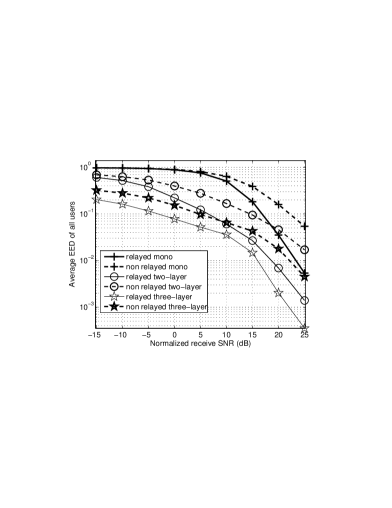
Figure 4: Comparison of the proposed relay-aided multicast approach with the reported counterparts in term of the average EED (P1) under the same transmit power at the source and relay.

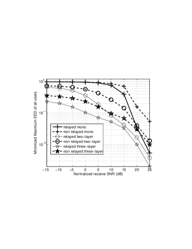
Figure 5: Minimized EED of the worst user of different schemes (P2) under the same transmit power at the source and relay.

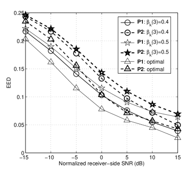
Figure 6: Performance comparison of optimized power allocation parameters versus randomly selected ones under the same transmit power at the source and relay. For non-optimal power vectors at the source and relay, $\beta_{k}(3)$ ($k=s,r$) is given (equal to $0.4$ or $0.5$) with the locally optimized $\beta_{k}^{o}(1)$ and $\beta_{k}^{o}(2)$ subject to the constraint that $\beta_{k}^{o}(1)+\beta_{k}^{o}(2)\leq 1-\beta_{k}(3)$.

TABLE II: Optimized power allocation parameters for three-level decode-and-forward (DF) relay aided JSCC system

Normalized SNR	Average EED		Worst EED
	$\boldsymbol{\beta_{s}^{*}}$	$\boldsymbol{\beta_{r}^{*}}$	$\boldsymbol{\beta_{s}^{*}}$	$\boldsymbol{\beta_{r}^{*}}$
-15dB	$\approx(0.9,0.1)$	$\approx(0.9,0.1)$	$\approx(0.9,0.1)$	$\approx(0.95,0.05)$
0dB	$\approx(0.75,0.2)$	$\approx(0.7,0.25)$	$\approx(0.84,0.15)$	$\approx(0.8,0.2)$
15dB	$\approx(0.61,0.3)$	$\approx(0.58,0.3)$	$\approx(0.8,0.15)$	$\approx(0.74,0.2)$

VI Conclusions

The paper studied a relay-aided joint source-channel coding (JSCC) multicast network containing a source, a decode-and-forward (DF) relay, and multiple receivers. A novel EED model for a general $L$-layer scalably coded source over fading channels was provided, which was further taken as the performance metric for the formulated optimization problems to determine a few key parameters such as resource allocation of different resolution layers at the source and relay. A novel programming algorithm was developed to obtain a good sub-optimal solution with guaranteed convergence. The case study results showed that the proposed relay aided multi-resolution design yields merits in suppressed EED against its counterparts in all the considered scenarios. In particular, we found that with more resolutions the EED performance could be considerably improved due to finer granularity of quality provisioning in presence of a large number of receivers with multi-user channel diversity.

Appendix A Derivation of Error Probability of Hierarchical Constellations

Here we derive the symbol error probability of each layer of the two-layer QPSK/QPSK as an example. It is noted that other hierarchical modulation cases can be similarly derived, and hence here we only focus on the two-layer QPSK/QPSK superimposed case as shown in Fig. 3 for brevity. We shall firstly derive the symbol error rate of the base layer and then decode the enhancement layer after applying SIC for the base layer. Assuming that $E$ is the average transmit energy for each hierarchical modulated symbol, we have $E_{1}=\beta E$ assigned to the base layer symbol and $E_{2}=(1-\beta)E$ assigned to the enhancement layer symbol. In addition, let $h$ be the instantaneous channel gain. Hence, the received symbol energy for the base layer and the enhancement layer are $hE_{1}$ and $hE_{2}$ respectively.

The coordinates of each superimposed symbol can be split into the abscissa and ordinate components, which are independently distorted by AWGN with its two-sided power spectral density $N_{0}/2$. The coordinates of the $16$ points in the constellation diagram, $(x_{i},x_{j}^{\prime})$, are independent normal variables with the following means and variances:

$$x_{i}\sim N(\pm\sqrt{\frac{hE_{1}}{2}}\pm\sqrt{\frac{hE_{2}}{2}},\frac{N_{0}}{2})$$

$$x_{j}^{\prime}\sim N(\pm\sqrt{\frac{hE_{1}}{2}}\pm\sqrt{\frac{hE_{2}}{2}},\frac{N_{0}}{2})$$

A-A Symbol Error Rate of Base Layer

For the base layer of the two-layer QPSK/QPSK, the decision boundaries are the vertical axis for the abscissa region as well as the horizontal axis for the ordinate region. It is noted that, due to symmetry, only symbols in the first quadrant, namely, $s_{1}\rightarrow s_{4}$, are considered. For the abscissa region, the conditional base layer error probabilities given each transmitted SPC symbol can be determined and categorized into two cases as follows,

$$p_{err1|s_{q}}^{(1)}=\begin{cases}Q\left[\sqrt{\tfrac{2}{N_{0}}}\left(\sqrt{\frac{hE_{1}}{2}}-\sqrt{\tfrac{hE_{2}}{2}}\right)\right]&\text{if }q=1,3\\ Q\left[\sqrt{\tfrac{2}{N_{0}}}\left(\sqrt{\frac{hE_{1}}{2}}+\sqrt{\tfrac{hE_{2}}{2}}\right)\right]&\text{if }q=2,4.\end{cases}$$ (34)

Similarly for the ordinate region, the conditional base layer error probabilities given each transmitted SPC symbol are derived as follows,

$$p_{err2|s_{q}}^{(1)}=\begin{cases}Q\left[\sqrt{\tfrac{2}{N_{0}}}\left(\sqrt{\frac{hE_{1}}{2}}+\sqrt{\tfrac{hE_{2}}{2}}\right)\right]&\text{if }q=1,2\\ Q\left[\sqrt{\tfrac{2}{N_{0}}}\left(\sqrt{\frac{hE_{1}}{2}}-\sqrt{\tfrac{hE_{2}}{2}}\right)\right]&\text{if }q=3,4.\end{cases}$$ (35)

Provided the assumption that each point is equally likely transmitted, the base layer error probability of the 2-layer QPSK/QPSK given the instantaneous channel gain can then be given by,

$$p^{(1)}=\frac{1}{4}\sum_{q=1}^{4}\left(1-\left(1-p_{err1|s_{q}}^{(1)}\right)\left(1-p_{err2|s_{q}}^{(1)}\right)\right).$$ (36)

It is noted that the average error probability of the base layer can be obtained by averaging over the channel gain distribution and the details are omitted due to its simplicity.

A-B Symbol Error Rate of Enhancement Layer

Note that to successfully decode the enhancement layer, the receivers need successfully decode the base layer and apply SIC for the base layer before decoding the enhancement layer. For clarity, let B and E denote the events where the base and enhancement layers of one SPC symbol are correctly detected, respectively. Applying the definition of conditional probability, the SER of the enhancement layer ($L=2$) is expressed using the intersection probability of events B and E as follows:

$$p^{(2)} =1-P({\tt B}\cap{\tt E})=1-P({\tt B})P({\tt E}|{\tt B})$$

$$=1-\left(1-p^{(1)}\right)\left(1-p_{{\tt cond}}^{(2)}\right)$$ (37)

where $p^{(1)}$ is the SER of the base layer and $p_{{\tt cond}}^{(2)}$ is the conditional SER of the enhancement layer provided correct reception of the base layer. Noting that SIC is applied for the base layer, the received QPSK symbol of the enhancement layer only has an average energy of $hE_{2}$ remaining, its conditional SER hence is given by the standard symbol error equation for a QPSK demodulator as follows,

$$p_{{\tt cond}}^{(2)}=2Q\left[\sqrt{\frac{hE_{2}}{N_{0}}}\right]-Q\left[\sqrt{\frac{hE_{2}}{N_{0}}}\right]^{2}.$$ (38)

Incorporating (36) and (38) into (37), the SER of the enhancement layer given the instantaneous channel gain can hence be obtained. It is also noted that the average error probability of the enhancement layer can be obtained by averaging over the channel gain distribution and the details are omitted due to its simplicity.

In addition, it is worth noting that, similar derivations of SER can be applied to other hierarchical constellation cases and are omitted here for brevity.

Appendix B Detailed SER Analysis of JSCC

Here we present the error probability derivation, with the assumption that the power allocated to each layer is specified and the channel realizations are known. Conditional on the assumption that the lower $l-1$ layers have been decoded correctly, the associated conditional symbol error rate (SER) for the $l$th layer information over link $i$-$j$ can be computed and is denoted by $p_{ij,{\tt cond}}^{(l)}$ ($i=s,r$ and $j=r,d_{1},\ldots,d_{N}$). Taking into account the dependence of decoding of each layer symbols, the probability of the event that the lower $l-1$ layer symbols are decoded successfully while the decoder fails in decoding the $l$th layer symbol, is hence given by

$$\prod_{k=1}^{l-1}\left(1-p_{ij,{\tt cond}}^{(k)}\right)p_{ij,{\tt cond}}^{(l)}.$$

where $1-p_{ij,{\tt cond}}^{(k)}$ is the successful decoding probability of the $k$th layer symbol conditional on the successful decoding of the lower $k-1$ layer symbols. In addition, it is readily observed that, when the decoder fails in decoding the $k$th ($k<l$) layer symbol, the higher layer symbols (including the $l$th layer) are naturally lost. Taking into account all these scenarios, the exact SER of the $l$th information hence is given by

$$p_{ij}^{(l)}= \prod_{k=1}^{l-1}\left(1-p_{ij,{\tt cond}}^{(k)}\right)p_{ij,{\tt cond}}^{(l)}$$

$$+\sum_{p=1}^{l-1}\prod_{k=1}^{p-1}\left(1-p_{ij,{\tt cond}}^{(k)}\right)p_{ij,{\tt cond}}^{(p)},$$ (39)

where the first term denotes the event that the lower $l-1$ layers are successfully decoded while only the $l$th layer is lost in SIC decoding, and each element of the second term in summation denotes the event that the lower $p$th ($p<l$) layer symbol is lost in SIC decoding hence the higher $l$th layer is naturally lost. Specifically, we have

$$p_{ij}^{(l)}-p_{ij}^{(l-1)}=\prod_{k=1}^{l-1}\left(1-p_{ij,{\tt cond}}^{(k)}\right)p_{ij,{\tt cond}}^{(l)}$$

denoting the probability that only up to layer $l-1$ over link $i\rightarrow j$ is successfully decoded given the channel realization.

Since each destination node receives JSCC symbols via both the direct and relay links which are decoded separately, the E2E SER of up to layer $l$ at the end of the second slot at $d_{n}$, given the realized link gains, denoted by $p_{err,d_{n}}^{(l)}$, is hence given in 3.

By averaging over the distribution of all the associated channel power gains, the expected E2E SER of up to layer $l$ at $d_{n}$ is therefore given by,

$$\bar{p}_{err,d_{n}}^{(l)}= \iiint\limits_{h_{sd_{n}},h_{sr},h_{rd_{n}}}\,p_{err,d_{n}}^{(l)}(h_{sd_{n}},h_{sr},h_{rd_{n}})f_{h}(h_{sd_{n}})$$

$$\,\,\,f_{h}(h_{rd_{n}})f_{h}(h_{sr})\,\mathrm{d}h_{sd_{n}}\,\mathrm{d}h_{sr}\,\mathrm{d}h_{rd_{n}}$$ (40)

Recall that $f_{h}(h_{ij})$ is the pdf of the channel power gain over link $i\rightarrow j$.

Appendix C EED of $L$-Resolution Scalable Source

Here the EED of an $L$-resolution scalable source over a memoryless broadcast channel with a finite size of codebook for each layer is derived. As shown in Fig. 2, $\boldsymbol{z}$ denotes a $M$-dimensional real-valued vector source over the Euclidean space $\Lambda$ with its pdf $f(\boldsymbol{z})$. The associated variance per dimension is hence determined by $\int_{\Lambda}||\boldsymbol{z}||^{2}f(\boldsymbol{z}){\it d\boldsymbol{z}}/M$. Note that here $\boldsymbol{z}$ is transmitted as an $L$-resolution scalably encoded source over a discrete memoryless broadcast channel and characterized by a transition matrix with its transitional probability $Pr\{\boldsymbol{\hat{r}}|\boldsymbol{r}\}$, where $\boldsymbol{\hat{r}}$ is the channel output and $\boldsymbol{r}$ is the channel input.

Due to its scalably encoding nature, the Euclidean space $\Lambda$ is first partitioned into $N_{1}$ disjoint regions for the base layer, denoted by $A_{k}$ ($k=1,\ldots,N_{1}$) where $N_{1}$ is the number of codeword vectors for the base layer, i.e., the size of the codebook for the base layer. For the first enhancement layer, each of the $N_{1}$ disjoint regions is partitioned into $N_{2}$ disjoint regions, denoted by $A_{ik}$ ($i=1,\ldots,N_{1}$ and $k=1,\ldots,N_{2}$) where $N_{2}$ is the number of codeword vectors for the first enhancement layer. Similarly, the Euclidean space can be repeatedly partitioned into more disjoint regions for the higher enhancement layers. For the $(L-1)$th enhancement layer, each of the $\prod_{i=1}^{L-1}N_{i}$ regions is partitioned into $N_{L}$ disjoint regions, denoted by $A_{i_{1}\cdots i_{L}}$ ($i_{l}=1,\ldots,N_{l}$ and $l=1,\ldots,L$) where $N_{l}$ is the number of codeword vectors for the $l-1$th enhancement layer, i.e., the size of the codebook for the $l-1$th enhancement layer. The vector associated with the region $A_{i_{1}\cdots i_{L}}$ is denoted by $\boldsymbol{z}_{i_{1}\cdots i_{L}}$. The original source is therefore represented by the index vector $(i_{1},\ldots,i_{L})$ where $i_{k}$ represents the $k$th layer, i.e., the $(k-1)$th enhancement layer if $k>1$ and the base layer if $k=0$.

Let $\pi_{t}(i_{1},\ldots,i_{L})=(r_{1},\ldots,r_{L})$ be a one-to-one mapping from the index vector to the channel input vector. Let the output vector be $(\hat{r}_{1},\ldots,\hat{r}_{L})$ where $\hat{r}_{k}\in\{r_{k},e\}$ and $e$ denotes detection error. As defined in Sec III-C, $\hat{p}_{err,{\tt L}_{j}}$ is the detection error probability of up to layer $j$, hence is given by

$$\hat{p}_{err,{\tt L}_{j}}= \sum_{k=1}^{j-1}\hat{p}_{err,{\tt L}_{k}}+Pr\{\hat{r}_{1}=r_{1},\ldots,\hat{r}_{j-1}=r_{j-1},r_{j}=e\},$$

$$\quad j=1,\ldots,L.$$ (41)

Note that each channel input vector $(r_{1},\ldots,r_{L})$ is uniformly distributed over $m_{e}=\prod_{i=1}^{L}N_{i}$, we have

$$\hat{p}_{err,{\tt L}_{1}}=\frac{1}{m_{e}}\sum_{\boldsymbol{r}}Pr\{\hat{r_{1}}=e|\boldsymbol{r}\},$$ (42)

$$\hat{p}_{err,{\tt L}_{l}}=\sum_{i=1}^{l-1}\hat{p}_{err,{\tt L}_{i}}+\frac{1}{m_{e}}\sum_{\boldsymbol{r}}Pr\{(r_{1},\ldots,r_{l-1},\hat{r_{l}}=e)|\boldsymbol{r}\},$$

$$\quad\quad\quad\quad\quad l=2,\ldots,L.$$ (43)

Given the $L$-layer output $\boldsymbol{\hat{r}}$, there are $L+1$ possible outputs:

$1$)$E[\boldsymbol{z}]$ if $\hat{r}_{1}=e$;

$l$)$z_{1\rightarrow l-1}$ if $\hat{r}_{1}\neq e,\ldots,\hat{r}_{l-1}\neq e,\hat{r}_{l}=e$; $\quad l=2,\ldots,L$

$L+1$)$z_{1\rightarrow L}$ if $\boldsymbol{\hat{r}}\neq e$.

The associated crossover error probabilities are hence given by,

$$p_{e}^{\pi_{t}}(E[\boldsymbol{z}]|\boldsymbol{z})=Pr\{r_{1}=e|\boldsymbol{r}\},$$ (44)

$$p_{e}^{\pi_{t}}(z_{1\rightarrow l-1}|\boldsymbol{z})=Pr\{r_{1},\ldots,r_{l-1},r_{l}=e|\boldsymbol{r}\},$$

$$\quad\quad\quad\quad\quad\quad\quad\quad l=2,\ldots,L,$$ (45)

$$p_{e}^{\pi_{t}}(z_{1\rightarrow L}|\boldsymbol{z})=Pr\{\boldsymbol{\hat{r}}\neq e|\boldsymbol{r}\}.$$ (46)

where $E[\boldsymbol{z}]$ is proved to be optimal when error is found at the base layer in [10]. Note also that EED is the mean squared error distortion between the original source $\boldsymbol{z}$ and the output $\boldsymbol{\hat{z}}\in\{E[\boldsymbol{z}],z_{1\rightarrow l}\}$ ($l=1,\ldots,L$). Therefore, with the error probability derived above, it is given as follows,

$$D_{{\tt L}_{L}}^{\pi_{t}}= \frac{1}{M}\sum_{\boldsymbol{z}}\int_{\boldsymbol{z}\in\Lambda}||z_{1\rightarrow L}-\boldsymbol{z}||^{2}p_{e}^{\pi_{t}}(z_{1\rightarrow L}|\boldsymbol{z})f(\boldsymbol{z})\textit{d}\boldsymbol{z}+\cdots$$

$$+\frac{1}{M}\sum_{\boldsymbol{z}}\int_{\boldsymbol{z}\in\Lambda}||z_{1\rightarrow l}-\boldsymbol{z}||^{2}p_{e}^{\pi_{t}}(z_{1\rightarrow l}|\boldsymbol{z})f(\boldsymbol{z})\textit{d}\boldsymbol{z}$$

$$+\cdots+\frac{1}{M}\sum_{\boldsymbol{z}}\int_{\boldsymbol{z}\in\Lambda}||\boldsymbol{z}||^{2}p_{e}^{\pi_{t}}(E[\boldsymbol{z}]|\boldsymbol{z})f(\boldsymbol{z})\textit{d}\boldsymbol{z}$$

$$= \left(1-\hat{p}_{err,{\tt L}_{L}}\right)\frac{1}{M}\sum_{\boldsymbol{z}}\int_{\boldsymbol{z}\in\Lambda}||z_{1\rightarrow L}-\boldsymbol{z}||^{2}f(\boldsymbol{z})\textit{d}\boldsymbol{z}+\cdots$$

$$+\left(\hat{p}_{err,{\tt L}_{l+1}}-\hat{p}_{err,{\tt L}_{l}}\right)\frac{1}{M}\sum_{\boldsymbol{z}}\int_{\boldsymbol{z}\in\Lambda}||z_{1\rightarrow l}-\boldsymbol{z}||^{2}f(\boldsymbol{z})\textit{d}\boldsymbol{z}$$

$$+\cdots+\hat{p}_{err,{\tt L}_{1}}\frac{1}{M}\sum_{\boldsymbol{z}}\int_{\boldsymbol{z}\in\Lambda}||\boldsymbol{z}||^{2}f(\boldsymbol{z})\textit{d}\boldsymbol{z}$$

$$= D_{Q_{L}}\left(1-\hat{p}_{err,{\tt L}_{L}}\right)+\sum_{l=1}^{L-1}D_{Q_{l}}\left(\hat{p}_{err,{\tt L}_{l+1}}-\hat{p}_{err,{\tt L}_{l}}\right)$$

$$+\sigma^{2}\hat{p}_{err,{\tt L}_{1}}$$ (47)

where (47) follows from the definition of $\hat{p}_{err,{\tt L}_{l}}$ and $D_{Q_{l}}$ denotes the quantization distortion of the reconstruction of the $l$-layer resolution.

References

- [1] C. T. K. Ng, D. Gunduz and A. J. Goldsmith, ``Recursive power allocation in gaussian layered broadcast coding with successive refinement," in Proc. IEEE Int. Conf. Communi. (ICC'07), pp. 889-896, 2007.
- [2] C. Tian, A. Steiner and S. Shamai, ``Successive refinement via broadcast: optimizing expected distortion of a gaussian source over a gaussian fading channel," IEEE Trans. Inf. Theory, vol. 54, no. 7, pp. 2903-2918, Jul. 2008.
- [3] V. Kostina and S. Verd . ``Lossy joint source-channel coding in the finite block length regime". In Proc. IEEE Int. Symp. Inf. Theory (ISIT'12), pp. 1553-1557, July. 2012.
- [4] D. Gunduz, E. Erkip, A. Goldsmith and H. V. Poor, ``Reliable joint source-channel cooperative transmission over relay networks." IEEE Trans. Inf. Theory, vol. 59, no. 4, pp. 2442-2458, Apr. 2013.
- [5] C. Gene, and A. Zakhor. ``Bit allocation for joint source/channel coding of scalable video." IEEE Trans. Image Processing, vol. 9, no. 3, pp. 340-356, Sep. 2000.
- [6] L. P. Kondi, F. Ishtiaq, and A. K. Katsaggelos. ``Joint source-channel coding for motion-compensated DCT-based SNR scalable video." IEEE Trans. Image Processing, vol. 11, no. 9, pp. 1043-1052, Nov. 2002.
- [7] A. Jain, D. Gunduz, S. R. Kulkarni, H. V. Poor and S. Verdu. ``Energy-distortion tradeoffs in Gaussian joint source-channel coding problems". IEEE Trans. Inf. Theory, vol. 58, no. 5, pp. 3153-3168, May. 2012.
- [8] M. P. Wilson, K. Narayanan and G. Caire. ``Joint source channel coding with side information using hybrid digital analog codes". IEEE Trans. Inf. Theory, vol. 56, no. 10, pp. 4922-4940, Oct. 2010.
- [9] X. Zhou, M. Cheng, K. Anwar and T. Matsumoto. ``Distributed joint source-channel coding for relay systems exploiting spatial and temporal correlations". In IEEE Proc. Wireless Advanced (WiAd'12), pp. 79-84. Jun. 2012.
- [10] X. Yu, H. Wang and E.-H. Yang. ``Design and analysis of optimal noisy channel quantization with random index assignment." IEEE Trans. Inf. Theory, vol. 56, no. 11, pp. 5796-5804, Nov. 2010.
- [11] J. Ho, and P.-H. Ho. ``On transmission of multiresolution gaussian sources over noisy relay networks." IEEE Trans. Wireless Communi., vol. 12, no. 7, pp. 3170-3179, Jul. 2013.
- [12] W. Ji, Z. Li and Y. Chen. ``Joint source-channel coding and optimization for layered video broadcasting to heterogeneous devices". IEEE Trans. Multimedia, vol. 14, no. 2, pp. 443-455, Feb. 2012.
- [13] D. Persson, J. Kron, M. Skoglund and E. G. Larsson. ``Joint source-channel coding for the MIMO broadcast channel" IEEE Trans. Sig. Processing, vol. 60, no. 4, pp. 2085-2090, Apr. 2011.
- [14] H. Kim, P. C. Cosman, and L. B. Milstein. ``Superposition coding based cooperative communication with relay selection." In 2010 Conf. Record of the Forty Fourth Asilomar Conf. on Signals, Systems and Computers, (ASILOMAR'10), pp. 892-896, 2010.
- [15] E. Pajala, T. Isotalo, A. Lakhzouri, E. S. Lohan and M. Renfors. ``An improved simulation model for Nakagami- fading channels for satellite positioning applications". 3rd Workshop on Position, Navigation and Communi., Hannover, Germany, pp. 81-89, Mar, 2006.
- [16] T. M. Cover, ``Broadcast channels," IEEE Trans. Inf. Theory, vol. IT-18, pp. 2-14, Jan. 1972.
- [17] W. H. R. Equitz and T. M. Cover, ``Successive refinement of information, IEEE Trans. Inf. Theory, vol. 37, no. 2, pp. 269 275, Mar. 1991.
- [18] A. Lapidoth, ``Nearest neighbor decoding for additive non-gaussian noise channels, IEEE Trans. Inform. Theory, vol. 42, pp. 1520-1529, Sep. 1996.
- [19] R. Tandra and A. Sahai. ``Is interference like noise when you know its codebook?" IEEE Int. Symp. Inf. Theory (ISIT'06), pp. 2220-2224, July. 2006.
- [20] V. Singh. ``On superposition coding for wireless broadcast channels". Master's thesis, KTH, Stockholm, Sweden, 2005.
- [21] P. K. Vitthaladevuni and M. S. Alouini. ``BER computation of 4/M-QAM hierarchical constellations". IEEE Trans. Broadcasting, vol. 47, no. 3, pp. 228-239, Mar. 2001.
- [22] J. G. Prokais, Digital Communications, 3rd ed. New York: McGraw-Hill, 1995.
- [23] S. Boyd and L. Vandenberghe, Convex Optimization. Cambridge, UK: Cambridge University Press, 2004.
- [24] R. M. Freund, ``Subgradient Optimization, Generalized Programming, and Nonconvex Duality." Massachusetts Institute of Technology, 2004.
- [25] D. P. Bertsekas, ``Convexification procedures and decomposition methods for nonconvex optimization problems." Journal of Optimization Theory and Applications, vol. 29, no. 2 pp. 169-197, 1979.