Bayesian correction of $H(z)$ data uncertainties

Abstract

We compile 41 $H(z)$ data from literature and use them to constrain O$\Lambda$CDM and flat $\Lambda$CDM parameters. We show that the available $H(z)$ suffers from uncertainties overestimation and propose a Bayesian method to reduce them. As a result of this method, using $H(z)$ only, we find, in the context of O$\Lambda$CDM, $H_{0}=69.5\pm 2.5\mathrm{\,km\,s^{-1}Mpc^{-1}}$, $\Omega_{m}=0.242\pm 0.036$ and $\Omega_{\Lambda}=0.68\pm 0.14$. In the context of flat $\Lambda$CDM model, we have found $H_{0}=70.4\pm 1.2\mathrm{\,km\,s^{-1}Mpc^{-1}}$ and $\Omega_{m}=0.256\pm 0.014$. This corresponds to an uncertainty reduction of up to 30% when compared to the uncorrected analysis in both cases.

I Introduction

Measurements of the expansion of the Universe are a central subject in the modern cosmology. In 1998, observations of type Ia supernovae riess1997 ; perlmutter gave strong evidences of a transition epoch between decelerated and accelerated expansion. Those evidences are also consistent with data from Baryon Acoustic Oscillations (BAO) measurements and the Cosmic Microwave Background Anisotropies (CMB).

Among the many viable candidates to explain the cosmic acceleration, the cosmological constant $\Lambda$ explains very well great part of the current observations and it is also the simplest candidate. It gave to the model formed by cosmological constant plus cold dark matter, the $\Lambda$CDM model, the status of standard model in cosmology. On the other hand, the $\Lambda$ term presents important conceptual problems in its core, e.g., the huge inconsistency of the quantum derived and the cosmological observed values of energy density, the so-called cosmological constant problem weinberg89 . Hence, despite of its observational success, the composition and the history of the universe is still a question that needs further investigation.

Precise measurements of the cosmic expansion may be obtained through the SNe observations. Although they furnish stringent cosmological constraints, they are not directly measuring the expansion rate $H(z)$ but its integral in the line of sight. Today, three distinct methods are producing direct measurements of $H(z)$ namely, through differential dating of the cosmic chronometers Simon05 ; Stern10 ; Moresco12 ; Zhang12 ; Moresco15 ; MorescoEtAl16 , BAO techniques Gazta09 ; Blake12 ; Busca12 ; AndersonEtAl13 ; Font-Ribera13 ; Delubac14 and correlation function of luminous red galaxies (LRGs) Chuang13 ; Oka13 , which does not rely on the nature of space-time geometry between the observed object and us.

In this work, we treat the $\Lambda$CDM model expansion history as a generative model for the $H(z)$ data Hogg .However, considering a goodness-of-fit criterion, we discuss a possible overestimation in the uncertainty in the current $H(z)$ data and we propose a new generative model to $H(z)$ data, in order to take into account this overestimation.

This article is structured as follows. In Section II, we discussed the basic features of the $\Lambda$CDM model. In section III, we review the $H(z)$ data available on the literature and compile a sample with 41 data.

In Section IV, we discuss the goodness of fit of $\Lambda$CDM with $H(z)$ data and in Section V we discuss a method to treat $H(z)$ uncertainties and apply it to $\Lambda$CDM with spatial curvature. In subsection V.1, we apply the same method to flat $\Lambda$CDM. In Section VI we compare corrected and uncorrected models by using a Bayesian criterion and in Section VII we compare our results with other $H(z)$ analyses. Finally, in Section VIII, we summarize the results.

II Cosmic Dynamics of $\Lambda$CDM Model

We start by considering the homogeneous and isotropic FRW line element (with $c=1$):

$$ds^{2}=dt^{2}-a^{2}(t)\left(\frac{dr^{2}}{1-kr^{2}}+r^{2}d\theta^{2}+r^{2}{\rm sin}^{2}\theta d\phi^{2}\right),$$ (1)

where $a$ is the scale factor, $(r,\theta,\phi)$ are comoving coordinates and the spatial curvature parameter $k$ can assume values $-1$, $+1$ or $0$.

In this background, the Einstein Field Equations (EFE) with a cosmological constant are given by

$$8\pi G\rho=3\frac{\dot{a}^{2}}{a^{2}}+3\frac{k}{a^{2}}-\Lambda$$ (2)

$$-8\pi Gp=2\frac{\ddot{a}}{a}+\frac{\dot{a}^{2}}{a^{2}}+\frac{k}{a^{2}}-\Lambda$$ (3)

where $\rho$ and $p$ are total density and pressure of the cosmological fluid and $\Lambda$ is cosmological constant. We may write the Friedmann equation (2) in terms of the observable redshift $z$, which relates to scale factor as $a=\frac{a_{0}}{1+z}$:

$$H^{2}=\frac{8\pi G(\rho+\rho_{\Lambda})}{3}-k(1+z)^{2},$$ (4)

where $\rho_{\Lambda}=\frac{\Lambda}{8\pi G}$ and $H\equiv\frac{\dot{a}}{a}$ is the expansion rate. The EFE include energy conservation, so we may deduce the continuity equation from Eqs. (2)-(3):

$$\dot{\rho}_{i}+3H(\rho_{i}+p_{i})=0,$$ (5)

where $(\rho_{i},p_{i})$ stand for each fluid, be it dark matter, baryons, radiation, neutrinos, cosmological constant or anything else that does not exchange energy. For dark matter and baryons, we have $p_{i}\sim 0$, so they evolve with $\rho_{i}\propto a^{-3}$, cosmological constant has constant $\rho_{\Lambda}$ and radiation and neutrinos follow $\rho_{i}\propto a^{-4}$, so they may be neglected in our work, as we are interested in low redshifts (up to $z\sim 2$). So, we may write for our components of interest:

$$\rho_{m} = \rho_{m0}(1+z)^{3}$$ (6)

$$\rho_{\Lambda} = \rho_{\Lambda 0}$$ (7)

where $\rho_{m}$ stands for dark matter+baryons. So, the Friedmann equation can be written:

$$\left(\frac{H}{H_{0}}\right)^{2}=\frac{8\pi G\rho_{m0}(1+z)^{3}}{3H_{0}^{2}}+\frac{8\pi G\rho_{\Lambda 0}}{3H_{0}^{2}}-\frac{k(1+z)^{2}}{H_{0}^{2}}$$ (8)

and by defining the density parameters $\Omega_{i}\equiv\frac{\rho_{i0}}{\rho_{c0}}$, where $\rho_{c0}\equiv\frac{3H_{0}^{2}}{8\pi G}$ and $\Omega_{k}\equiv-\frac{k}{a_{0}^{2}H_{0}^{2}}$, we may write

$$\left(\frac{H}{H_{0}}\right)^{2}=\Omega_{m}(1+z)^{3}+\Omega_{k}(1+z)^{2}+\Omega_{\Lambda}$$ (9)

from which we deduce the normalization condition $\Omega_{m}+\Omega_{\Lambda}+\Omega_{k}=1$, or $\Omega_{k}=1-\Omega_{m}-\Omega_{\Lambda}$, so we actually have three free parameters on this equation ($\Omega_{m},\Omega_{\Lambda},H_{0}$). Finally, we may write for $H(z)$:

$$H(z)=H_{0}\left[\Omega_{m}(1+z)^{3}+(1-\Omega_{m}-\Omega_{\Lambda})(1+z)^{2}+\Omega_{\Lambda}\right]^{\frac{1}{2}}$$ (10)

As usual, we will call this model, where we allow for spatial curvature, O$\Lambda$CDM. The standard, concordance flat $\Lambda$CDM model has $\Omega_{k}=0$, thus:

$$H(z)=H_{0}\left[\Omega_{m}(1+z)^{3}+1-\Omega_{m}\right]^{\frac{1}{2}}$$ (11)

III $H(z)$ data

Hubble parameter data as function of redshift yields one of the most straightforward cosmological tests because it is inferred from astrophysical observations alone, not depending on any background cosmological models.

At the present time, the most important methods for obtaining $H(z)$ data are (i) through “cosmic chronometers”, for example, the differential age of galaxies (DAG) Simon05 ; Stern10 ; Moresco12 ; Zhang12 ; Moresco15 ; MorescoEtAl16 , (ii) measurements of peaks of acoustic oscillations of baryons (BAO) Gazta09 ; Blake12 ; Busca12 ; AndersonEtAl13 ; Font-Ribera13 ; Delubac14 and (iii) through correlation function of luminous red galaxies (LRG) Chuang13 ; Oka13 .

The data we work here are a combination of two compilations: Sharov and Vorontsova SharovVor14 and Moresco et al. MorescoEtAl16 . SharovVor14 adds 6 $H(z)$ data in comparison to Farooq and Ratra farooq2013 compilation, which had 28 measurements. Moresco et al. MorescoEtAl16 , on their turn, have added 7 new $H(z)$ measurements in comparison to SharovVor14 . By combining both datasets, we arrive at 41 $H(z)$ data, as can be seen on Table 1 and Figure 1.

$z$	$H(z)$	$\sigma_{H}$	Reference
0.070	69	19.6	Zhang12
0.090	69	12	Simon05
0.120	68.6	26.2	Zhang12
0.170	83	8	Simon05
0.179	75	4	Moresco12
0.199	75	5	Moresco12
0.200	72.9	29.6	Zhang12
0.240	79.69	6.65	Gazta09
0.270	77	14	Simon05
0.280	88.8	36.6	Zhang12
0.300	81.7	6.22	Oka13
0.350	82.7	8.4	Chuang13
0.352	83	14	Moresco12
0.3802	83	13.5	MorescoEtAl16
0.400	95	17	Simon05
0.4004	77	10.02	MorescoEtAl16
0.4247	87.1	11.2	MorescoEtAl16
0.430	86.45	3.68	Gazta09
0.440	82.6	7.8	Blake12
0.4497	92.8	12.9	MorescoEtAl16
0.4783	80.9	9	MorescoEtAl16

$z$	$H(z)$	$\sigma_{H}$	Reference
0.480	97	62	Stern10
0.570	92.900	7.855	AndersonEtAl13
0.593	104	13	Moresco12
0.6	87.9	6.1	Blake12
0.68	92	8	Moresco12
0.73	97.3	7.0	Blake12
0.781	105	12	Moresco12
0.875	125	17	Moresco12
0.88	90	40	Stern10
0.9	117	23	Simon05
1.037	154	20	Moresco12
1.300	168	17	Simon05
1.363	160	22.6	Moresco15
1.43	177	18	Simon05
1.53	140	14	Simon05
1.75	202	40	Simon05
1.965	186.5	50.4	Moresco15
2.300	224	8	Busca12
2.34	222	7	Delubac14
2.36	226	8	Font-Ribera13

Table 1: 41 Hubble parameter versus redshift data.

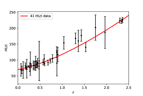
Figure 1: 41 $H(z)$ data and corresponding best fit $\Lambda$CDM model.

From these data, we perform a $\chi^{2}$-statistics, generating the $\chi^{2}$ function of free parameters:

$$\chi^{2}=\sum_{i=1}^{41}\left[\frac{H_{0}E(z_{i},\Omega_{m},\Omega_{\Lambda})-H_{i}}{\sigma_{Hi}}\right]^{2}$$ (12)

where $E(z)\equiv\frac{H(z)}{H_{0}}$ and $H(z)$ is given by Eq. (10).

IV Data analysis and goodness of fit

In order to minimize the $\chi^{2}$ function (12) and find the constraints over the free parameters $(H_{0},\Omega_{m},\Omega_{\Lambda})$, we have sampled the likelihood $\mathscr{L}\propto e^{-\chi^{2}/2}$ through Monte Carlo Markov Chain (MCMC) analysis. A simple and powerful MCMC method is the so called Affine Invariant MCMC Ensemble Sampler by Goodman and Weare GoodWeare , which was implemented in Python language with the emcee software by Foreman-Mackey et al. ForemanMackey13 . This MCMC method has the advantage over simple Metropolis-Hasting (MH) methods of depending on only one scale parameter of the proposal distribution and on the number of walkers, while MH methods in general depend on the parameter covariance matrix, that is, it depends on $n(n+1)/2$ tuning parameters, where $n$ is dimension of parameter space. The main idea of the Goodman-Weare affine-invariant sampler is the so called “stretch move”, where the position (parameter vector in parameter space) of a walker (chain) is determined by the position of the other walkers. Foreman-Mackey et al. modified this method, in order to make it suitable for parallelization, by splitting the walkers in two groups, then the position of a walker in one group is determined by only the position of walkers of the other group.

We used the freely available software emcee to sample from our likelihood in our 3-dimensional parameter space. We have used flat priors over the parameters. In order to plot all the constraints in the same figure, we have used the freely available software getdist, in its Python version. The results of our statistical analyses from Eq. (12) correspond to the red lines in Fig. 3 and Table 2. From this analysis, we have obtained $\chi^{2}_{\nu}=\frac{\chi^{2}_{min}}{\nu}=18.551/38=0.48819$, where $\nu=n-p$ is number of degrees of freedom.

As it is well known Bevington ; Vuolo , when one analyses the probability distribution of $\chi^{2}_{\nu}$ it has an expected value $\chi^{2}_{\nu}=1$. $\chi^{2}_{\nu}$ values very far from this are unlikely. High $\chi^{2}_{\nu}$ values may indicate underestimation of uncertainties or poor fitting of the model, while low values of $\chi^{2}_{\nu}$ indicate, in general, overestimation of uncertainties. The $\chi^{2}_{\nu}$ distribution is given by

$$h_{\nu}(\chi^{2}_{\nu})=\frac{\nu^{\frac{\nu}{2}}(\chi^{2}_{\nu})^{\frac{1}{2}(\nu-2)}e^{-\frac{\nu}{2}\chi^{2}_{\nu}}}{2^{\nu/2}\Gamma(\nu/2)},$$ (13)

where $\Gamma$ is complete gamma function. It can be shown that the mean $\chi^{2}_{\nu}$ is given by $\overline{\chi^{2}_{\nu}}=1$, while the mode is given by $\widehat{\chi^{2}_{\nu}}=1-\frac{2}{\nu}$. In the limit of a large sample and few parameters, both converge to the same value $\chi^{2}_{\nu}\approx 1$. From (13), we may also define the cumulative distribution function (cdf) or probability of obtaining a value of $\chi^{2}_{\nu}$ as low as $Q$ as:

$$P(\chi^{2}_{\nu}<Q)\equiv\int_{0}^{Q}h_{\nu}(Q^{\prime})dQ^{\prime}$$ (14)

In order to realize how low is the $\chi^{2}_{\nu}$ value we have obtained, namely, $\chi^{2}_{\nu}=0.48819$, we have plotted the pdf $h_{\nu}(\chi^{2}_{\nu})$ (13) and the cdf (14) for $\nu=38$ in Fig. 2.

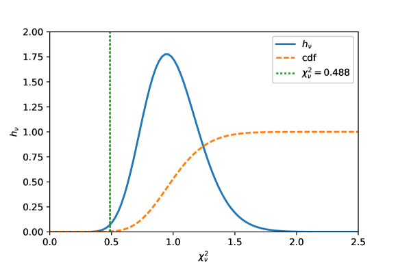
Figure 2: $h_{\nu}(\chi^{2}_{\nu})$ and corresponding cdf for $\nu=38$.

As one may see in this figure, the probability of obtaining $\chi^{2}_{\nu}$ as low as $\chi^{2}_{\nu}=0.488$ for $\nu=38$ is quite low. In fact, by calculating the integral (14), we have obtained $P(\chi^{2}_{\nu}<0.48819)=0.3342\%$. It indicates, thus, a very low and unlikely $\chi^{2}$ value, which, in turn, from Eq. (12) indicates overestimated $H(z)$ uncertainties.

V $H(z)$ uncertainties correction

How one may try to correct uncertainties? Ideally, at the level of obtaining data, new methods less prune to errors are to be used. In fact, in general, data coming from BAO and Lyman $\alpha$ have smaller errors than data coming from differential ages. However, not being able to reobtaining the data, or reanalyzing then through new methods, we are left with the available data. Then, nothing can be done? From the Bayesian viewpoint, not necessarily. In fact, we may view the data as a collection of $(z_{i},H_{i},\sigma_{Hi})$. Very often, we are interested in a likelihood given by $\mathcal{L}=Ne^{-\chi^{2}/2}$, where $N$ is only a normalization constant and one is interested in maximize the likelihood, which is equivalent to minimize the $\chi^{2}$. Let us recall from where this expression comes from.

As explained in Hogg , the likelihood may be seen as an objective function, that is, a function that represents monotonically the quality of the fit. Given a scientific problem at hand, as fitting a model to the data, one must define this objective function that represents this “goodness of fit”, then try to optimize it in order to determine the best free parameters of the model that describe the data.

Hogg et al. Hogg argues that the only choice of the objective function that is truly justified – in the sense that it leads to probabilistic inference, is to make a generative model for the data. We may think of the generative model as a parameterized statistical procedure to reasonably generate the given data.

For instance, assuming Gaussian uncertainties in one dimension, we may create the following generative model: Imagine that the data really come from a function $y=f(x,\theta)$ given by the model, and that the only reason that any data point deviates from this model is that to each of the true $y$ values a small $y$-direction offset has been added, where that offset was drawn from a Gaussian distribution of zero mean and known variance $\sigma_{y}^{2}$. In this model, given an independent position $x_{i}$, an uncertainty $\sigma_{yi}$, and free parameters $\theta$, the frequency distribution $p(y_{i}|x_{i},\sigma_{yi},\theta)$ for $y_{i}$ is

$$p(y_{i}|x_{i},\sigma_{yi},\theta)=\frac{1}{(2\pi)^{1/2}\sigma_{yi}}\,\exp\left[-\frac{(y_{i}-f(x_{i},\theta))^{2}}{2\,\sigma_{yi}^{2}}\right]\quad,$$ (15)

Thus, if the data points are independently drawn, the likelihood $\mathscr{L}$ is the product of conditional probabilities

$$\mathscr{L}=\prod_{i=1}^{n}\ p(y_{i}|x_{i},\sigma_{yi},\theta)\quad.$$ (16)

Taking the logarithm,

$$\ln\mathscr{L}=-\frac{1}{2}\sum_{i=1}^{n}\left[\frac{(y_{i}-f(x_{i},\theta))^{2}}{\sigma_{yi}^{2}}+\ln(2\pi\sigma_{yi}^{2})\right]$$ (17)

In equation above, the second term $-\frac{1}{2}\sum_{i}\ln(2\pi\sigma_{yi}^{2})$ is in general absorbed in the likelihood normalization constant, because the variances $\sigma_{yi}^{2}$ are considered fixed by the data. Here, we consider $\sigma_{i}$ as parameters to be obtained by optimization of the objective function $\mathscr{L}$. As discussed in Hogg , it can be considered a correct procedure from the Bayesian point of view, although an involved one, and the obtained $\sigma_{i}$ can be quite prior dependent.

In order to avoid having more free parameters than data, here we consider the $\sigma_{i}$ to be all overestimated by a constant factor $f$, thus, $\sigma_{i,true}=f\sigma_{i}$. It can be seen just as a simplifying hypothesis, a first order correction. More elaborated methods could be cluster the data in some groups, then correct the $\sigma_{i}$ for each group. However, as explained in Hogg , it is not an easy task to separate good data from bad data, and not necessarily the bad data are the ones with bigger uncertainties. So, we limit ourselves here with just one overall correction factor, next we conclude if this a good approximation. We treat $f$ as a free parameter, then we constrain it in a joint analysis with the cosmological parameters, similar to what is made in current SNe Ia analyses Union2 ; Union2.1 ; Betoule . For $\Lambda$CDM, then, our set of free parameters now is $\theta=(H_{0},\Omega_{m},\Omega_{\Lambda},f)$. A simpler but less justified hypothesis would be simply find the value for $f$ which provides $\chi^{2}_{\nu}\equiv 1$. However, as we expect $\chi^{2}_{\nu}$ to have some variance, such a procedure is not much trustworthy. With $f$ as a free parameter, it may include some uncertainty into the analysis, when compared to the standard, uncorrected analysis, but at the same time, it may also reduce the cosmological parameters uncertainties.

Instead of Eq. (17), we must work here with the following objective function:

$$\ln\mathscr{L}=-\frac{1}{2}\sum_{i=1}^{n}\left\{\frac{\left[H_{i}-H(z_{i},H_{0},\Omega_{m},\Omega_{\Lambda})\right]^{2}}{f^{2}\sigma_{Hi}^{2}}+\ln(2\pi f^{2}\sigma_{Hi}^{2})\right\}$$ (18)

By maximizing the above likelihood, we find not only the best fit cosmological parameters, but also the best correction factor $f$ which will furnish the best model to describe the data. By doing the same procedure of last section, now with the additional parameter $f$, we find the constraints shown by the black lines on Figure 3.

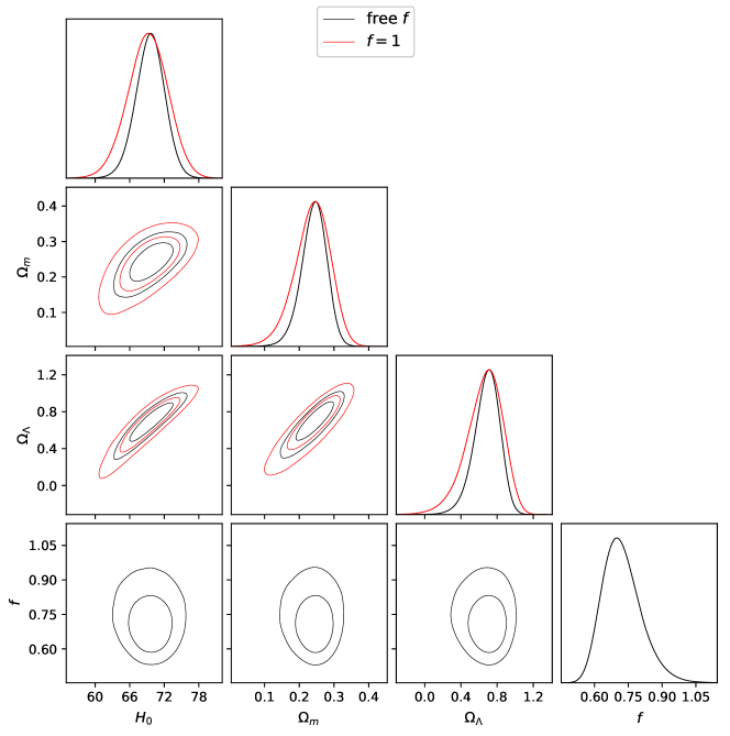
Figure 3: The results of statistical analysis for O$\Lambda$CDM model. $H_{0}$ in km/s/Mpc. Diagonal: Marginalized constraints from $H(z)$ data for each parameter. Below diagonal: Marginalized contours constraints for each indicated combination of parameters, with contours for 68.3% and 95.4% confidence levels.

From Figure 3, we may already see the difference in the parameter space if we introduce the $f$ parameter. The corrected contours (black lines) are narrower then the uncorrected contours (red lines). It can be quantified by the parameter constraints shown on Table 2.

	$H(z)$ only		$H(z)+H_{0}$
Parameter	Uncorrected	Corrected	Uncorrected	Corrected
$H_{0}$	$69.1\pm 3.5$	$69.5\pm 2.5$	$72.4\pm 1.5$	$72.5\pm 1.1$
$\Omega_{m}$	$0.237\pm 0.051$	$0.242\pm 0.036$	$0.267\pm 0.038$	$0.268\pm 0.028$
$\Omega_{\Lambda}$	$0.66\pm 0.20$	$0.68\pm 0.14$	$0.825^{+0.11}_{-0.095}$	$0.831\pm 0.073$
$f$	–	$0.723^{+0.084}_{-0.085}$	–	$0.728^{+0.067}_{-0.098}$

Table 2: Mean values of parameters of O$\Lambda$CDM model from $H(z)$ data, without uncertainties correction and with uncertainties correction factor $f$. Uncertainties correspond to 68% c.l.

As can be seen on Table 2, $\sigma_{H0}$ has been reduced from 3.5 to 2.5, $\sigma_{\Omega_{m}}$ has been reduced from 0.051 to 0.036 and $\sigma_{\Omega_{\Lambda}}$ has been reduced from 0.20 to 0.14. The mean value for $f$ was $f=0.723^{+0.084}_{-0.085}$. An interesting feature we may see from Fig. 3, is that the $f$ parameter is much uncorrelated to cosmological parameters. It explains the small shift on mean values of cosmological parameters from Table 2. Saying in another way, the central values of cosmological parameters are insensitive to overall shifts on $H_{i}$ uncertainties, but their variances are directly affected by $f$.

V.1 Flat $\Lambda$CDM

For completeness, as flat $\Lambda$CDM model is favoured from many observations, in this section we analyse this model similarly to O$\Lambda$CDM. Eq. (10) now reads:

$$H(z)=H_{0}\left[\Omega_{m}(1+z)^{3}+1-\Omega_{m}\right]^{\frac{1}{2}}$$ (19)

The results of this analysis may be seen on Fig. 4 and Table 3.

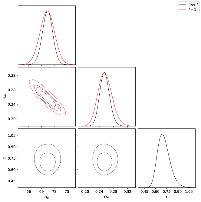
Figure 4: The results of statistical analysis for flat $\Lambda$CDM model. $H_{0}$ in km/s/Mpc. Diagonal: Marginalized constraints from $H(z)$ data for each parameter. Below diagonal: Marginalized contours constraints for each indicated combination of parameters, with contours for 68.3% and 95.4% confidence levels.

As one may see from Fig. 4, $f$ is again uncorrelated to cosmological parameters, so it does not change their central values.

	$H(z)$ only		$H(z)+H_{0}$
Parameter	Uncorrected	Corrected	Uncorrected	Corrected
$H_{0}$	$70.3\pm 1.7$	$70.4\pm 1.2$	$71.8\pm 1.2$	$71.80\pm 0.89$
$\Omega_{m}$	$0.257\pm 0.020$	$0.256\pm 0.014$	$0.243^{+0.014}_{-0.015}$	$0.242\pm 0.011$
$f$	–	$0.714\pm 0.082$	–	$0.728^{+0.066}_{-0.096}$

Table 3: Mean values of parameters of Flat $\Lambda$CDM model from $H(z)$ data, without uncertainties correction and with uncertainties correction factor $f$. Uncertainties correspond to 68% c.l.

As one may see on Table 3, the $H_{0}$ uncertainty, for instance, is reduced from 1.7 to 1.2, which now corresponds to 1.7% relative uncertainty. $\Omega_{m}$ uncertainty has reduced from 0.020 to 0.014.

VI Bayesian Criterion Comparison

Here, we use the Bayesian Information Criterion (BIC) Schwarz78 ; bic-ccdm in order to compare the models with uncertainties corrections and without uncertainties correction. As an approximation for the Bayesian Evidence (BE) Trotta08 , BIC is useful because it is, in general, easier to calculate. BIC is given by:

$$\mathrm{BIC}=-2\ln\mathscr{L}_{max}+p\ln n$$ (20)

where $\mathscr{L}_{max}$ is the likelihood maximum and $p$ is the number of free parameters. The two models we want to compare are: $M_{1}:f=1$, that is, $\Lambda$CDM model without uncertainties correction is enough to describe the data; and $M_{2}:f\neq 1$ such that some correction $f$ to uncertainties is necessary in order to $\Lambda$CDM explain the $H(z)$ data. We may write the log-likelihood as:

$$\ln\mathscr{L}=-\frac{1}{2}\left[\frac{\chi^{2}}{f^{2}}+\sum_{i=1}^{n}\ln(2\pi f^{2}\sigma_{i}^{2})\right]$$ (21)

where $\chi^{2}$ is the uncorrected $\chi^{2}\equiv\sum_{i=1}^{n}\frac{\left[H_{i}-H(z_{i},H_{0},\Omega_{m},\Omega_{\Lambda})\right]^{2}}{\sigma_{Hi}^{2}}$. To calculate BIC, we must find the maximum of $\ln\mathscr{L}$. By deriving (21) with respect to $f$:

$$\frac{\partial\ln\mathscr{L}}{\partial f}=-\frac{1}{f}\left[n-\frac{\chi^{2}}{f^{2}}\right]$$ (22)

When it vanishes, we find the best fit:

$$\hat{f}=\sqrt{\frac{\chi^{2}_{min}}{n}}$$ (23)

From (20) and (23) we find:

$$\mathrm{BIC}_{1}=\chi^{2}_{min}+\sum_{i=1}^{n}\ln(2\pi\sigma_{i}^{2})+p_{1}\ln n$$ (24)

$$\mathrm{BIC}_{2}=n+n\ln\left(\frac{2\pi\chi^{2}_{min}}{n}\right)+\sum_{i=1}^{n}\ln(\sigma_{i}^{2})+p_{2}\ln n$$ (25)

where $p_{j}$ is the number of free parameters in $M_{j}$. So:

$$\Delta\mathrm{BIC}=\mathrm{BIC}_{1}-\mathrm{BIC}_{2}=\chi^{2}_{min}-n\ln\left(\chi^{2}_{min}\right)+(n-p_{2}+p_{1})\ln n-n$$ (26)

For $p_{1}=3$ and $p_{2}=4$, it simplifies to:

$$\Delta\mathrm{BIC}=\chi^{2}_{min}-n\ln\left(\chi^{2}_{min}\right)+(n-1)\ln n-n$$ (27)

For $n=41$ and $\chi^{2}_{min}=18.551$, it yields: $\Delta\mathrm{BIC}=6.352$. As discussed in bic-ccdm , for example, values of $\Delta\mathrm{BIC}>5$ corresponds to a decisive or strong statistical difference. That is, by this criterion, the model $M_{1}$ (no correction) may be discarded against model $M_{2}$ (with correction).

VII Comparison with other $H(z)$ data analyses

Farooq and Ratra farooq2013 have constrained O$\Lambda$CDM model with 28 $H(z)$ data and two possible priors over $H_{0}$. With the most stringent prior, namely, the one from Riess et al. (2011) Riess11 , they have found, at 2$\sigma$, $0.20\leq\Omega_{m}\leq 0.44$ and $0.62\leq\Omega_{\Lambda}\leq 1.14$. We have found $0.13\leq\Omega_{m}\leq 0.34$ and $0.23\leq\Omega_{\Lambda}\leq 1.04$ for 41 $H(z)$ data without correction and $0.162\leq\Omega_{m}\leq 0.31$ and $0.38\leq\Omega_{\Lambda}\leq 0.96$ with the $f$ correction. By considering the prior from Riess et al. (2011), namely, $H_{0}=73.8\pm 2.4\mathrm{\,km\,s^{-1}\,Mpc^{-1}}$, we have found $0.18\leq\Omega_{m}\leq 0.34$ and $0.57\leq\Omega_{\Lambda}\leq 1.04$ without correction and $0.21\leq\Omega_{m}\leq 0.32$ and $0.65\leq\Omega_{\Lambda}\leq 0.99$ with the $f$ correction.

With 34 $H(z)$ data, Sharov and Vorontsova SharovVor14 find a more stringent result, namely, $H_{0}=70.26\pm 0.32$, $\Omega_{m}=0.276^{+0.009}_{-0.008}$ and $\Omega_{\Lambda}=0.769\pm 0.029$. However, they have combined $H(z)$ data with SNe Ia and BAO data, which is beyond the scope of our present work. However, by comparing their result with our Table 2, we may see that both constraints are compatible at 1$\sigma$ c.l.

Moresco et al. have used their compilation of 30 $H(z)$ data combined with $H_{0}$ from Riess et al. (2011) Riess11 to constrain the transition redshift from deceleration to acceleration, in the context of O$\Lambda$CDM zt :

$$z_{t}=\left[\frac{2\Omega_{\Lambda}}{\Omega_{m}}\right]^{1/3}-1$$ (28)

They have found $z_{t}=0.64^{+0.11}_{-0.07}$. By using the present 41 $H(z)$ data, we find $z_{t}=0.77\pm 0.22$ without correction and $z_{t}=0.78\pm 0.15$ with the $f$ correction. The results are in fully agreement without the correction and are compatible at 2$\sigma$ c.l. with the $f$ correction. We have mentioned the mean value for $z_{t}$, while Moresco et al. refers to the best fit value.

The constraints over $H_{0}$ are quite stringent today from many observations RiessEtAl16 ; Planck16 . However, there is some tension among $H_{0}$ values estimated from different observations BernalEtAl16 , so we choose not to use $H_{0}$ in our main results here, Figs. 3 and 4. We combine $H(z)+H_{0}$ only in Tables 2 and 3 and in the present section, using Riess et al. (2011) Riess11 result, in order to compare with other earlier analyses.

VIII Conclusion

In this work, we have compiled 41 $H(z)$ data and proposed a new method to better constrain models using $H(z)$ data alone, namely, by reducing overestimated uncertainties through a Bayesian approach. The Bayesian Information Criterion was used to show the need for correcting $H(z)$ data uncertainties. The uncertainties in the parameters were quite reduced when compared with methods of parameter estimation without correction and we have obtained an estimate of an overall correction factor in the context of O$\Lambda$CDM and flat $\Lambda$CDM models.

Further investigations may include constraining other cosmological models or trying to optimally group $H(z)$ data and then correcting uncertainties.

- (1) A. G. Riess et al. [Supernova Search Team Collaboration], Astron. J. 116, 1009 (1998). [astro-ph/9805201].
- (2) S. Perlmutter et al. [Supernova Cosmology Project Collaboration], Astrophys. J. 517, 565 (1999). [astro-ph/9812133].
- (3) Weinberg S., Rev. Mod. Phys. 61, 1 (1989).
- (4) J. Simon, L. Verde and R. Jimenez, Constraints on the redshift dependence of the dark energy potential, Phys. Rev. D 71 (2005) 123001 [astro-ph/0412269].
- (5) D. Stern, R. Jimenez, L. Verde, M. Kamionkowski and S. A. Stanford, Cosmic chronometers: constraining the equation of state of dark energy. I: measurements, J. of Cosmology and Astropart. Phys. 02 (2010) 008 [arXiv:0907.3149].
- (6) M. Moresco et al., Improved constraints on the expansion rate of the Universe up to 1.1 from the spectroscopic evolution of cosmic chronometers, J. of Cosmology and Astropart. Phys. 8 (2012) 006 [arXiv:1201.3609].
- (7) C. Zhang, H. Zhang, S. Yuan, T. J. Zhang and Y. C. Sun, Res. Astron. Astrophys. 14, no. 10, 1221 (2014) [arXiv:1207.4541 [astro-ph.CO]].
- (8) M. Moresco, Raising the bar: new constraints on the Hubble parameter with cosmic chronometers at z 2,, Mon. Not. Roy. Astron. Soc. 450 (2015) L16 [arXiv:1503.01116].
- (9) M. Moresco et al., JCAP 1605 (2016) no.05, 014 [arXiv:1601.01701 [astro-ph.CO]].
- (10) E. Gaztañaga, A. Cabre, L. Hui, Clustering of Luminous Red Galaxies IV: Baryon Acoustic Peak in the Line-of-Sight Direction and a Direct Measurement of , Mon. Not. Roy. Astron. Soc. 399(3) (2009) 1663 [arXiv:0807.3551].
- (11) C. Blake et al., The WiggleZ Dark Energy Survey: Joint measurements of the expansion and growth history at , Mon. Not. Roy. Astron. Soc. 425(1) (2012) 405 [arXiv:1204.3674].
- (12) N. G. Busca et al., Baryon Acoustic Oscillations in the Ly forest of BOSS quasars, Astron. and Astrop. 552 (2013) A96 [arXiv:1211.2616].
- (13) L. Anderson et al., Mon. Not. Roy. Astron. Soc. 439, no. 1, 83 (2014) [arXiv:1303.4666 [astro-ph.CO]].
- (14) A. Font-Ribera et al., Quasar-Lyman Forest Cross-Correlation from BOSS DR11: Baryon Acoustic Oscillations, J. of Cosmology and Astroparticle Phys. 05 (2014) 027 [arXiv:1311.1767].
- (15) T. Delubac et al. [BOSS Collaboration], Astron. Astrophys. 574 (2015) A59 [arXiv:1404.1801 [astro-ph.CO]].
- (16) C.H. Chuang and Y. Wang, Modeling the Anisotropic Two-Point Galaxy Correlation Function on Small Scales and Improved Measurements of , , and from the Sloan Digital Sky Survey DR7 Luminous Red Galaxies, Mon. Not. Roy. Astron. Soc. 435(1) (2013) 255 [arXiv:1209.0210].
- (17) A. Oka et al., Simultaneous constraints on the growth of structure and cosmic expansion from the multipole power spectra of the SDSS DR7 LRG sample, Mon. Not. Roy. Astron. Soc. 439(3) (2014) 2515 [arXiv:1310.2820].
- (18) D. W. Hogg, J. Bovy and D. Lang, arXiv:1008.4686 [astro-ph.IM].
- (19) J. A. S. Lima, J. F. Jesus, R. C. Santos and M. S. S. Gill, arXiv:1205.4688 [astro-ph.CO].
- (20) G. S. Sharov and E. G. Vorontsova, JCAP 1410 (2014) no.10, 057 [arXiv:1407.5405 [gr-qc]].
- (21) O. Farooq and B. Ratra, Astrophys. J. Lett., 766, L7, (2013).
- (22) Goodman, J. and Weare, J., 2010, Comm. App. Math. Comp. Sci., v. 5, 1, 65
- (23) D. Foreman-Mackey, D. W. Hogg, D. Lang and J. Goodman, 2013, Publ. Astron. Soc. Pac. 125 306 [arXiv:1202.3665 [astro-ph.IM]].
- (24) R. Allison and J. Dunkley, Mon. Not. Roy. Astron. Soc. 437, 2014, no.4, 3918 [arXiv:1308.2675 [astro-ph.IM]].
- (25) A. Lewis and S. Bridle, 2002, Phys. Rev. D 66, 103511 [astro-ph/0205436].
- (26) P. R. Bevington and D. K. Robinson, “Data Reduction and Error Analysis for the Physical Sciences”, 2003, McGraw-Hill Book Company.
- (27) J. H. Vuolo, “Fundamentos da Teoria de Erros” (in Portuguese), 1996, Ed. Edgard Blücher.
- (28) R. Amanullah et al., Astrophys. J. 716 (2010) 712 [arXiv:1004.1711 [astro-ph.CO]].
- (29) N. Suzuki et al. [Union 2.1], Astrophys. J. 746, 85 (2012) [arXiv:1105.3470 [astro-ph.CO]].
- (30) M. Betoule et al. [SDSS Collaboration], Astron. Astrophys. 568 (2014) A22 [arXiv:1401.4064 [astro-ph.CO]].
- (31) G. Schwarz, Ann. Stat., 5, (1978), 461.
- (32) J. F. Jesus, R. Valentim and F. Andrade-Oliveira, JCAP 1709 (2017) no.09, 030 [arXiv:1612.04077 [astro-ph.CO]].
- (33) R. Trotta, Contemp. Phys. 49 (2008) 71 [arXiv:0803.4089 [astro-ph]].
- (34) A. G. Riess et al., Astrophys. J. 730 (2011) 119 Erratum: [Astrophys. J. 732 (2011) 129] [arXiv:1103.2976 [astro-ph.CO]].
- (35) A. G. Riess et al., Astrophys. J. 826 (2016) no.1, 56 [arXiv:1604.01424 [astro-ph.CO]].
- (36) P. A. R. Ade et al. [Planck Collaboration], Astron. Astrophys. 594 (2016) A13 [arXiv:1502.01589 [astro-ph.CO]].
- (37) J. L. Bernal, L. Verde and A. G. Riess, JCAP 1610 (2016) no.10, 019 [arXiv:1607.05617 [astro-ph.CO]].