Nonparametric density estimation from observations with multiplicative measurement errors

Abstract

In this paper we study the problem of pointwise density estimation from observations with multiplicative measurement errors. We elucidate the main feature of this problem: the influence of the estimation point on the estimation accuracy. In particular, we show that, depending on whether this point is separated away from zero or not, there are two different regimes in terms of the rates of convergence of the minimax risk. In both regimes we develop kernel–type density estimators and prove upper bounds on their maximal risk over suitable nonparametric classes of densities. We show that the proposed estimators are rate–optimal by establishing matching lower bounds on the minimax risk. Finally we test our estimation procedures on simulated data.

T1The research is supported by the Russian Academic Excellence Project “5-100” and by the Israel Science Foundation (ISF) research grant 361/15.

and

t1Faculty of Mathematics, Duisburg-Essen University, D-45127 Essen, Germany. t2Department of Statistics, University of Haifa, Haifa 31905, Israel. t3National Research University Higher School of Economics, Moscow.

1 Introduction

Problem formulation and background

In this paper we study the problem of nonparametric density estimation from observations with multiplicative measurements errors. In particular, assume that we observe a sample $Y_{1},\ldots,Y_{n}$ generated by the model

$$Y_{i}=X_{i}\eta_{i},\;\;\;i=1,\ldots,n,$$ (1.1)

where $X_{1},\ldots,X_{n}$ are independent identically distributed (i.i.d) random variables with density $f_{X}$, and $\eta_{1},\ldots,\eta_{n}$ are i.i.d. random variables, independent of $X_{1},\ldots,X_{n}$, with known density $g$. Our goal is to estimate the value of $f_{X}$ at a single given point $x_{0}$ from observations $Y_{1},\ldots,Y_{n}$. If $f_{Y}$ stands for the density of $Y=X\eta,$ then

$$f_{Y}(y)=[f_{X}\star g](y) := \int_{-\infty}^{\infty}\frac{1}{x}f_{X}(y/x)g(x)\mathrm{d}x$$ (1.2)

$$= \int_{-\infty}^{\infty}\frac{1}{x}g(y/x)f_{X}(x)\mathrm{d}x,\;\;\;y\in{\mathbb{R}}.$$

Thus $f_{Y}$ is a scale mixture of $g$, and estimation of $f_{X}$ from observations $Y_{1},\ldots,Y_{n}$ can be viewed as the problem of demixing of a scale mixture.

The outlined estimation problem appears in the literature in various contexts. First, the model (1.1) with normal errors $\eta_{i}$ and positive random variables $X_{i}$ represents a stochastic volatility model without drift. In this context estimation of the volatility density $f_{X}$ from observations $Y_{1},\ldots,Y_{n}$ was studied by Van Es et al. [19], Van Es & Speij [18] and Belomestny & Shoenmakers [6].

Second, if $(\eta_{i})$ are uniformly distributed on $[0,1]$ then the corresponding model (1.1) is referred to as the multiplicative censoring model. In this setting Vardi [20] studied the problem of estimating the distribution function of $X$ under the assumption that two samples $Y_{1},\ldots,Y_{n}$ and $X_{n+1},\ldots,X_{n+m}$ are available. The aforementioned paper develops a nonparametric maximum likelihood estimator; large sample properties of this estimator are studied in Vardi & Zhang [21]. The problem of density estimation in the multiplicative censoring model was considered in Andersen & Hansen [1] and Comte & Dion [8], where estimators based on orthogonal series have been developed. Kernel density estimators were studied in Asgharian et al. [4] and Brunel et al. [7]. We also refer the reader to the recent work by Belomestny et al. [5] where a generalized multiplicative censoring model with $(\eta_{i})$ being beta-distributed random variables was introduced and studied; see also references therein.

Third, as mentioned above, the outlined problem can be viewed as the problem of demixing of a scale mixture. Closely related problems of estimating mixing densities were considered by Zhang [23], [24] and Loh & Zhang [15]. In particular, the paper [23] develops Fourier techniques for estimating mixing densities in location models, while [24] and [15] focus on estimating mixing densities in discrete exponential family models. However we are not aware of works on estimating mixing densities in the context of scale models. Finally, we also mention related results on estimating regression functions with multiplicative errors–in–variables that are reported in Iturria et al. [13].

A naive approach to the problem of density estimation in the model with multiplicative errors is based on reduction to the additive measurement error model. In particular, assuming that $X_{i}$’s and $\eta_{i}$’s are positive random variables and taking logarithms of the both sides of (1.1), we come to the additive model $Y_{i}^{\prime}=X^{\prime}_{i}+\eta^{\prime}_{i}$, where $Y_{i}^{\prime}=\ln Y_{i}$, $X^{\prime}_{i}=\ln X_{i}$ and $\eta^{\prime}_{i}=\ln\eta_{i}$. In this model, the density $f_{X^{\prime}}$ of $X^{\prime}$ can be estimated using the well developed methodology for additive deconvolution problems (see, e.g., [23] and [10]), and then an estimator for $f_{X}$ can be obtained using the inverse transformation $f_{X}(x)=(1/x)f_{X^{\prime}}(\ln x)$. This idea has been utilized in Van Es & Spreij [18] and Van Es et al. [19]. However, several questions about applicability of this approach arise. First, it can be used only if $X$ and $\eta$ are nonnegative random variables. Second, it does not provide an estimator of $f_{X}$ at the origin $x=0$ since the inverse transformation is not well–defined there. Third, even if this approach is applicable, it is not clear whether the resulting estimator possesses the desired optimality properties.

In contrast to voluminous literature on density deconvolution in the model with additive measurement errors, the problem of density estimation from observations with multiplicative errors was studied to a much lesser extent. In fact, it was considered only for specific distributions of errors $(\eta_{i})$ such as normal, uniform or beta, and the estimators proposed in the literature are tailored to a specific form of the error density $g$. In this context the following natural questions arise. How to estimate $f_{X}$ under general assumptions on the error density $g$? Which properties of the error density $g$ do affect the estimation accuracy, and what is the achievable accuracy in estimating $f_{X}$? What can be said about properties of the deconvolution estimators based on the logarithmic transformation of the data?

The main goal of the present paper is to develop optimal estimators of $f_{X}$ in a principled way under general assumptions on the error density $g$ and to provide answers to the questions raised above. Our approach makes use of the Mellin transform which, in view of its properties, is an appropriate tool for constructing estimators in this setting.

We adopt minimax framework for measuring estimation accuracy. Specifically, accuracy of an estimator $\hat{f}_{X}(x_{0})$ of $f_{X}(x_{0})$ is measured by the maximal risk

$${\cal R}_{n}[\hat{f}_{X};\Sigma]:=\sup_{f_{X}\in\Sigma}\Big{[}\mathbb{E}_{f_{X}}|\hat{f}_{X}(x_{0})-f_{X}(x_{0})|^{2}\Big{]}^{1/2},$$

where $\Sigma$ is a class of densities. Here and in what follows, $\mathbb{E}_{f_{X}}$ denotes the expectation with respect to the distribution of the observations $Y_{1},\ldots,Y_{n}$ when the unknown density of $X$ is $f_{X}$. The minimax risk is defined by

$${\cal R}_{n}^{*}[\Sigma]:=\inf_{\hat{f}_{X}}{\cal R}_{n}[\hat{f}_{X};\Sigma]=\inf_{\hat{f}_{X}}\sup_{f_{X}\in\Sigma}\Big{[}\mathbb{E}_{f_{X}}|\hat{f}_{X}(x_{0})-f_{X}(x_{0})|^{2}\Big{]}^{1/2},$$

where $\inf$ is taken over all possible estimators. Our goal is to develop an estimator $\hat{f}_{X}(x_{0})$ which is rate–optimal, i.e.,

$${\cal R}_{n}[\hat{f}_{X};\Sigma]\leq C_{n}{\cal R}_{n}^{*}[\Sigma],\;\;\;\sup_{n}C_{n}<\infty.$$

Main contributions

The main contributions of this work are as follows.

We elucidate the main feature of the multiplicative measurement errors setting: the influence of the estimation point $x_{0}$ on the achievable estimation accuracy. In particular, assuming that unknown density $f_{X}$ belongs to a local Hölder functional class in a vicinity of $x_{0}$, we show that, depending on the value of $x_{0}$, there are two different regimes in terms of the rates of convergence of the minimax risk. We develop a general method for estimating $f_{X}(x_{0})$ in these two regimes.

The first regime corresponds to the situation when the value of $x_{0}$ is separated away from zero. Here the achievable rate of convergence is primarily determined by the value of $x_{0}$, by the local smoothness of $f_{X}$, and by the ill–posedness of the integral transform in (1.2). The latter is characterized in terms of the rate at which the Mellin transform of $g$ decreases at infinity on a line parallel to the imaginary axis in the complex plane. It is worth noting that this characteristic is global in the sense that it is determined by the global behavior of the error density $g$ on its support. We construct a kernel–type estimator of $f_{X}(x_{0})$ and prove that it is rate–optimal in terms of dependence on the sample size $n$, parameters of the considered functional class $\Sigma$ and $x_{0}$. It turns out that the deconvolution estimator based on the logarithmic transformation of the data is a special case of the proposed estimation procedure. As a by–product of our general results, we demonstrate that if $x_{0}$ is separated away from zero, the random variables $X$ and $\eta$ are nonnegative, and $f_{X}$ belongs to a local Hölder class in a vicinity of $x_{0},$ then under certain conditions on $g$ the deconvolution estimator is rate–optimal. However, if $f_{X}$ satisfies some additional constraints, e.g., a moment condition, then the accuracy of the deconvolution estimator can be improved.

In the second regime, where $x_{0}=0$, completely different phenomena are observed. It turns out that in this case the achievable accuracy in estimating $f_{X}(0)$ is determined by smoothness of $f_{X}$ and by local behavior of $g$ in vicinity of the origin. Thus, in contrast to the first regime, the minimax rate depends only on local characteristics of $g$ and is not affected by the ill–posedness of the integral transform in (1.2). In particular, our results imply that if $g$ is bounded and does not vanish in a vicinity of the origin, then the minimax rate of convergence is only by a $\ln n$–factor worse than the one achievable in the problem of density estimation from direct observations. We also construct a rate–optimal estimator of $f_{X}(0)$ and prove a matching lower bound on the minimax risk.

Organization of the paper

The rest of the paper is organized as follows. In Section 2 we introduce notation, discuss some properties of the Mellin transform that are used throughout the paper and present an identifiability result. Section 3 deals with the setting when $x_{0}$ is separated away from zero; we construct estimators under different assumptions on the error density $g$ and present results on their accuracy over suitable classes of densities. Section 4 is devoted to the problem of estimating $f_{X}(0)$. A simulation study of the proposed estimators is presented in Section 5. Finally, proofs of main results are presented in Section 6 while proofs of auxiliary statements are given in Section 7.

2 Preliminaries

In this section we introduce notation and discuss basic properties of the Mellin transform that will be extensively used throughout the paper. This material can be found, e.g., in [16] and [22]. In addition, we present a result on identifiability of the distribution of $X$ in the model (1.1).

The Mellin transform

For a generic locally integrable function $u$ on $(0,\infty)$ the Mellin transform of $u$ is defined by

$$\widetilde{u}(z)={\cal M}[u;z]:=\int_{0}^{\infty}x^{z-1}u(x)\mathrm{d}x$$ (2.1)

for all $z\in\mathbb{C}$ such that the integral on the right hand side is absolutely convergent. The region of convergence $\Omega_{u}$ is an infinite vertical strip in the complex plane $\mathbb{C}$,

$$\Omega_{u}=\{z\in\mathbb{C}:a<{\rm Re}(z)<b\},\;\;a<b,$$

or a vertical line $\Omega_{u}=\{z:{\rm Re}(z)=c\}$ if $u(x)x^{c-1}\in{\mathbb{L}}_{1}({\mathbb{R}}_{+})$ for one $c\in{\mathbb{R}}$. For example, if $u(x)=O(x^{-a+\epsilon})$ as $x\to 0+$ and $u(x)=O(x^{-b-\epsilon})$ as $x\to\infty$ for some $\epsilon>0,$ then the integral in (2.1) converges absolutely and defines an analytic function $\widetilde{u}(z)$ on $\Omega_{u}=\{z:a<{\rm Re}(z)<b\}$.

The inversion formula for the Mellin transform is

$$u(x)=\frac{1}{2\pi i}\int_{c-i\infty}^{c+i\infty}x^{-z}\widetilde{u}(z)\,\mathrm{d}z,\;\;\;c\in\Omega_{u}\cap(-\infty,\infty).$$

Let $u(x)$ and $v(x)$ be functions such that the integral $I=\int_{0}^{\infty}u(x)v(x)\mathrm{d}x$ exists. Assume also that the Mellin transforms $\widetilde{u}(1-z)={\cal M}[u;1-z]$ and $\widetilde{v}(z)={\cal M}[v;z]$ have a common strip of analyticity, which will be the case when $I$ is absolutely convergent. Then for any line $\{z:\,{\rm Re}(z)=c\}$ in this common strip the Parseval formula is valid:

$$\int_{0}^{\infty}u(x)v(x)\mathrm{d}x=\frac{1}{2\pi i}\int_{c-i\infty}^{c+i\infty}\widetilde{u}(1-z)\widetilde{v}(z)\mathrm{d}z.$$

In particular, we get for $u=v$ and $c=\frac{1}{2}$,

$$\int_{0}^{\infty}u^{2}(x)\mathrm{d}x=\frac{1}{2\pi}\int_{-\infty}^{\infty}|\widetilde{u}(\tfrac{1}{2}+i\omega)|^{2}\mathrm{d}\omega.$$

It also holds

$$\int_{0}^{\infty}u^{2}(x)x^{2s-1}\mathrm{d}x=\frac{1}{2\pi}\int_{-\infty}^{\infty}|\widetilde{u}(s+i\omega)|^{2}\mathrm{d}\omega.$$ (2.2)

Let us mention the relation of the Mellin transform to a multiplicative convolution integral (1.2); this property is central in subsequent developments. Let $u$ and $v$ be defined on $[0,\infty)$, and let

$$[u\star v](y):=\int_{0}^{\infty}\frac{1}{x}u(x)v(y/x)\mathrm{d}x;$$

then

$$\widetilde{[u\star v]}(z)={\cal M}[u\star v;z]={\cal M}[u;z]{\cal M}[v;z]=\widetilde{u}(z)\widetilde{v}(z).$$

We shall use the Mellin transform techniques for functions defined on the whole real line. To this end, for a function $u$ on $(-\infty,\infty)$ we set

$$u^{+}(x):=\left\{\begin{array}[]{ll}u(x),&x\geq 0,\\ 0,&x<0\end{array}\right.\;\;\;\;\hbox{and}\;\;\;\;\;u^{-}(x):=\left\{\begin{array}[]{ll}u(-x),&x>0,\\ 0,&x\leq 0.\end{array}\right.$$ (2.3)

It is evident that with this notation $u(x)=u^{+}(x)$ for $x\geq 0$ and $u(x)=u^{-}(-x)$ for $x<0$. The one–sided Mellin transforms of function $u$ defined on $(-\infty,\infty)$ are given by

$$\widetilde{u}^{+}(z)=\int_{0}^{\infty}x^{z-1}u^{+}(x)\mathrm{d}x=\int_{0}^{\infty}x^{z-1}u(x)\mathrm{d}x,$$

$$\widetilde{u}^{-}(z)=\int_{0}^{\infty}x^{z-1}u^{-}(x)\mathrm{d}x=\int_{-\infty}^{0}(-x)^{z-1}u(x)\mathrm{d}x.$$

The Laplace and Fourier transforms

The bilateral Laplace transform of function $u$ on $(-\infty,\infty)$ is defined as

$$\widecheck{u}(z)={\cal L}[u;z]:=\int_{-\infty}^{\infty}u(x)e^{-zx}\mathrm{d}x,$$

and if the integral absolutely converges on a line $\{z:{\rm Re}(z)=c\},$ then the inverse Laplace transform is given by

$$u(x)=\frac{1}{2\pi i}\int_{c-i\infty}^{c+i\infty}\widecheck{u}(z)e^{zx}\mathrm{d}z.$$

The Fourier transform of $u$ is $\widehat{u}(\omega)={\cal F}[u;\omega]:={\cal L}[u;i\omega]=\widecheck{u}(i\omega)$.

Identifiability

In the model (1.1) we do not assume that the random variables $X$ and $\eta$ are nonnegative. This fact raises the question whether the distribution of $X$ is identifiable from the distribution of $Y$. The next statement provides a necessary and sufficient condition for the identifiability.

Lemma 1.

The probability density $f_{X}$ is identifiable from $f_{Y}$ if and only if $g(x)\neq g(-x)$ on a set of positive Lebesgue measure.

The proof of Lemma 1 is given in Section 7. It shows that the identifiability condition is equivalent to the requirement that $|[\widetilde{g}^{+}(z)]^{2}-[\widetilde{g}^{-}(z)]^{2}|$ is not zero for almost all $z$ in the common strip of analyticity of $\widetilde{g}^{+}$ and $\widetilde{g}^{-}$. Finally, we note that if one of the variables $X$ or $\eta$ is nonnegative, then the condition of identifiability is trivially fulfilled.

3 Estimation at a point separated away from zero

In this section we consider the problem of estimation of $f_{X}$ at a point $x_{0}$ separated away from zero.

3.1 Construction of estimator

We adopt the linear functional strategy for constructing our estimators. This strategy has been frequently used for solving ill–posed inverse problems (see, e.g., [12] and [2]). In our context, the main idea of this method is to find a pair of kernels, say, $K(x,y)$ and $L(x,y)$ such that:

• $\int_{-\infty}^{\infty}K(x,y)f_{X}(y)\mathrm{d}y$ approximates “well” the value $f_{X}(x)$ to be recovered;

• kernel $L(x,y)$ is related to $K(x,y)$ via the equation

  $$\int_{-\infty}^{\infty}K(x,y)f_{X}(y)\mathrm{d}y=\int_{-\infty}^{\infty}L(x,y)f_{Y}(y)\mathrm{d}y.$$ (3.1)

Then under (i) and (ii), the empirical estimator of the integral on the right hand side of (3.1) provides a sensible estimator for $f_{X}(x)$.

Kernel construction

Let $K:{\mathbb{R}}\to{\mathbb{R}}$ be a kernel function and for any positive real number $h$ define

$$K_{h}(x,y)=\left\{\begin{array}[]{ll}\tfrac{1}{xh}K\big{(}\tfrac{\ln(y/x)}{h}\big{)},&y/x>0,\\[5.69054pt] 0,&y/x<0.\end{array}\right.$$ (3.2)

Let $\widetilde{g}^{+}(z)={\cal M}[g^{+};z]$ and $\widetilde{g}^{-}(z)={\cal M}[g^{-};z]$ be the one–sided Mellin transforms of $g$, and let

$$\Omega_{g^{+}}\cap\Omega_{g^{-}}=:\{z\in\mathbb{C}:a<{\rm Re}(z)<b\}$$ (3.3)

be the common strip of their analyticity. Since $g$ is a probability density, we always have $a<1<b$; hence $\Omega_{g^{+}}\cap\Omega_{g^{-}}$ is non–empty – it always contains the line $\{z\in\mathbb{C}:{\rm Re}(z)=1\}$. We note that $\Omega_{g^{+}}$ and/or $\Omega_{g^{-}}$ can degenerate to this line. In this case, by convention, we put $a=1$, $b=1$, and corresponding open interval should be replaced by a singleton.

For $s\in(1-b,1-a)$ define

$$L_{s,h}(x,y)\\ :=\left\{\begin{array}[]{ll}{\displaystyle\frac{1}{2\pi ix}\int_{s-i\infty}^{s+i\infty}\Big{|}\frac{x}{y}\Big{|}^{z}\,\frac{\widecheck{K}(zh)\;\widetilde{g}^{+}(1-z)}{[\widetilde{g}^{+}(1-z)]^{2}-[\widetilde{g}^{-}(1-z)]^{2}}\,\mathrm{d}z,}&y/x>0,\\[17.07164pt] {\displaystyle-\frac{1}{2\pi ix}\int_{s-i\infty}^{s+i\infty}\Big{|}\frac{x}{y}\Big{|}^{z}\frac{\widecheck{K}(zh)\;\widetilde{g}^{-}(1-z)}{[\widetilde{g}^{+}(1-z)]^{2}-[\widetilde{g}^{-}(1-z)]^{2}}\,\mathrm{d}z,}&y/x<0.\end{array}\right.$$ (3.4)

For the time being, we suppose that the kernel $K$ and the error density $g$ are such that the function $L_{s,h}$ is well defined; the corresponding conditions on $K$ and $g$ will be formulated later. Several remarks on this definition are in order.

Remark 1.

• We can assume that the Laplace transform $\widecheck{K}(\cdot)$ of kernel $K$ is an entire function. This does not restrict generality since $K$ can be always chosen to satisfy this assumption.

• If $[\widetilde{g}^{+}(z)]^{2}-[\widetilde{g}^{-}(z)]^{2}\neq 0$ for all $z\in\Omega_{g^{+}}\cap\Omega_{g^{-}}$ then the integrands in (3.4) are analytic functions in $\{z\in\mathbb{C}:1-b<{\rm Re}(z)<1-a\}$. In this case the integrals in (3.4) do not depend on the integration path, and $L_{s,h}(x,y)$ does not depend on $s\in(1-b,1-a)$. If function $[\widetilde{g}^{+}(z)]^{2}-[\widetilde{g}^{-}(z)]^{2}$ has zeros in $\Omega_{g^{+}}\cap\Omega_{g^{-}}$ then the functions under the integral sign in (3.4) are meromorphic, and $L_{s,h}(x,y)$ depends on parameter $s$.

The relationship between kernels $L_{s,h}(x,y)$ and $K_{h}(x,y)$ in (3.4) and (3.2) is revealed in the following statement.

Lemma 2.

Let $K_{h}(x,y)$ be given by (3.2). Let $s\in(1-b,1-a)$ where $a$ and $b$ are given in (3.3), and suppose that the integrals on the right hand side of (3.4) are absolutely convergent. Then it holds that

$$\int_{-\infty}^{\infty}L_{s,h}(x,y)f_{Y}(y)\mathrm{d}y=\int_{-\infty}^{\infty}K_{h}(x,t)f_{X}(t)\mathrm{d}t.$$ (3.5)

The proof of Lemma 2 is given in Section 7. We note that relationship (3.5) is in full accordance with the linear functional strategy [cf. (3.1)]. Because $a<1<b$, it holds that $0\in(1-b,1-a)$; hence one can always choose $s=0$ in (3.4). This choice yields

$$L_{0,h}(x,y)=\left\{\begin{array}[]{ll}{\displaystyle\frac{1}{2\pi x}\int_{-\infty}^{\infty}\Big{|}\frac{x}{y}\Big{|}^{i\omega}\,\frac{\widehat{K}(\omega h)\;\widetilde{g}^{+}(1-i\omega)}{[\widetilde{g}^{+}(1-i\omega)]^{2}-[\widetilde{g}^{-}(1-i\omega)]^{2}}\,\mathrm{d}\omega,}&y/x>0,\\[17.07164pt] {\displaystyle-\frac{1}{2\pi x}\int_{-\infty}^{\infty}\Big{|}\frac{x}{y}\Big{|}^{i\omega}\frac{\widehat{K}(\omega h)\;\widetilde{g}^{-}(1-i\omega)}{[\widetilde{g}^{+}(1-i\omega)]^{2}-[\widetilde{g}^{-}(1-i\omega)]^{2}}\,\mathrm{d}\omega,}&y/x<0.\end{array}\right.$$

If $g$ is supported on $[0,\infty)$, then $\widetilde{g}^{-}=0$, $\widetilde{g}^{+}=\widetilde{g}$; in this case

$$L_{s,h}(x,y)=\frac{1}{2\pi ix}\int_{s-i\infty}^{s+i\infty}\Big{|}\frac{x}{y}\Big{|}^{z}\,\frac{\widecheck{K}(zh)}{\widetilde{g}(1-z)}\,\mathrm{d}z,\;\;\;y/x>0,$$ (3.7)

and $L_{s,h}(x,y)=0$ whenever $x/y<0$. In particular, for $s=0$ we have

$$L_{h}(x,y):=L_{0,h}(x,y)=\frac{1}{2\pi x}\int_{-\infty}^{\infty}\Big{|}\frac{x}{y}\Big{|}^{i\omega}\frac{\widehat{K}(\omega h)}{\widetilde{g}(1-i\omega)}\mathrm{d}\omega,\;\;\;y/x>0.$$ (3.8)

Estimator

For $|x_{0}|>0$ we define the estimator of $f_{X}(x_{0})$ by

$$\hat{f}_{s,h}(x_{0})=\frac{1}{n}\sum_{j=1}^{n}L_{s,h}(x_{0},Y_{j}),$$ (3.9)

where $L_{s,h}$ is given in (3.4), $h>0$ and $s\in(1-b,1-a)$ are two tuning parameters to be specified. In what follows with a slight abuse of notation we shall write $\hat{f}_{h}(x_{0}):=\hat{f}_{0,h}(x_{0})$ and $L_{h}(x,y):=L_{0,h}(x,y)$.

Note also that (3.5) implies

$$\mathbb{E}_{f_{X}}[\hat{f}_{s,h}(x_{0})]=\int_{-\infty}^{\infty}K_{h}(x_{0},t)f_{X}(t)\mathrm{d}t.$$

The latter formula is crucial for the analysis of the bias of $\hat{f}_{s,h}(x_{0}).$

3.2 Relation to the additive deconvolution problem

There is close connection between the kernel $L_{h}(x,y)=L_{0,h}(x,y)$ defined in (3.8) and kernels used in the additive deconvolution problems. Specifically, suppose that $X$ and $\eta$ are positive random variables, and let $\eta^{\prime}=\ln\eta$. If $g$ is the density of $\eta$, and $\widehat{g}$ is the corresponding characteristic function, then $g_{\eta^{\prime}}(x)=e^{x}g(e^{x})$ is the density of $\eta^{\prime}$, and the characteristic function of $\eta^{\prime}$ is $\widehat{g}_{\eta^{\prime}}(\omega)={\cal M}[g;1-i\omega]=\widetilde{g}(1-i\omega)$. Therefore the expression for $L_{h}(x,y)$ in (3.8) can be rewritten as

$$L_{h}(x,y)=\frac{1}{2\pi x}\int_{-\infty}^{\infty}\frac{\widehat{K}(\omega h)}{\widehat{g}_{\eta^{\prime}}(\omega)}e^{-i\omega(\ln y-\ln x)}\mathrm{d}\omega,\;\;\;x>0,\;y>0,$$

and the corresponding estimator of $f_{X}(x_{0})$ [cf. (3.9)] is

$$\hat{f}_{X}(x_{0})=\frac{1}{n}\sum_{j=1}^{n}L_{h}(x_{0},Y_{j})=\frac{1}{2\pi x_{0}n}\sum_{j=1}^{n}\int_{-\infty}^{\infty}\frac{\widehat{K}(\omega h)}{\widehat{g}_{\eta^{\prime}}(\omega)}e^{-i\omega(\ln Y_{j}-\ln x_{0})}\mathrm{d}\omega.$$ (3.10)

On the other hand, consider the additive deconvolution model for the logarithms, $Y^{\prime}=X^{\prime}+\eta^{\prime}$, where $Y^{\prime}=\ln Y$, $X^{\prime}=\ln X$ and $\eta^{\prime}=\ln\eta$. Then the standard deconvolution estimator of $f_{X^{\prime}}(t_{0})$ is of the form

$$\hat{f}_{X^{\prime}}(t_{0})=\frac{1}{2\pi n}\sum_{j=1}^{n}\int_{-\infty}^{\infty}\frac{\widehat{K}(\omega h)}{\widehat{g}_{\eta^{\prime}}(\omega)}e^{-i\omega(Y_{j}^{\prime}-t_{0})}\mathrm{d}\omega.$$

Since $f_{X^{\prime}}(t_{0})=e^{t_{0}}f_{X}(e^{t_{0}})$, we can estimate $f_{X}(x_{0})=\frac{1}{x_{0}}f_{X^{\prime}}(\ln x_{0})$ by

$$\hat{f}_{X}(x_{0}) = \frac{1}{x_{0}}\hat{f}_{X^{\prime}}(\ln x_{0})$$ (3.11)

$$= \frac{1}{2\pi x_{0}n}\sum_{j=1}^{n}\int_{-\infty}^{\infty}\frac{\widehat{K}(\omega h)}{\widehat{g}_{\eta^{\prime}}(\omega)}e^{-i\omega(Y_{j}^{\prime}-\ln x_{0})}\mathrm{d}\omega$$

which coincides with (3.10).

We conclude that if random variables $X$ and $\eta$ are positive, and the parameter $s$ of the estimator $\hat{f}_{s,h}(x_{0})$ in (3.9) is set to zero, then both approaches lead to the same estimator. Thus, the estimator (3.11) is a particular case of our estimator $\hat{f}_{s,h}(x_{0})$ defined in (3.9). We note however that tuning parameter $s$ adds some flexibility, and its proper choice can improve accuracy of $\hat{f}_{s,h}(x_{0})$ under suitable assumptions (see, e.g., Theorem 3 below).

3.3 Convergence analysis

We proceed with convergence analysis of the risk of the proposed estimator $\hat{f}_{s,h}(x_{0})$. In order to avoid unnecessary technicalities, from now on we will assume that $X$ and $\eta$ are nonnegative random variables, i.e.,

$${\rm supp}(g)\subseteq[0,\infty),\;\Omega_{g}=\{z\in\mathbb{C}:a<{\rm Re}(z)<b\},\;{\rm supp}(f_{X})\subseteq[0,\infty)$$ (3.12)

for some $a>0$ and $b>a$. Under these conditions the kernel $L_{s,h}(x,y)$ is given by (3.7).

Assumption (3.12) streamlines the presentation and, in fact, does not lead to loss of generality. In particular, the ensuing analysis of the risk of $\hat{f}_{s,h}(x_{0})$ remains valid for general random variables $X$ and $\eta$, provided that the conditions imposed in the sequel on the Mellin transform $\widetilde{g}$ of $g$ are replaced by the corresponding conditions on $([\widetilde{g}^{+}]^{2}-[\widetilde{g}^{-}]^{2})/\widetilde{g}^{+}$ and $([\widetilde{g}^{+}]^{2}-[\widetilde{g}^{-}]^{2})/\widetilde{g}^{-}$ [cf. (3.4)].

The risk of $\hat{f}_{s,h}(x_{0})$ will be analyzed under a local smoothness assumption on $f_{X}$ and two different sets of assumptions on the error density $g$.

Definition 1.

Let $\beta>0$, $A>0$, $x_{0}>0$ and $r>1$. We say that $f\in{\mathscr{H}}_{x_{0},r}(A,\beta)$ if $f$ is a probability density, that is, $\ell=\lfloor\beta\rfloor:=\max\{k\in{\mathbb{N}}_{0}:k<\beta\}$ times continuously differentiable, and $\max_{k=1,\ldots,\ell}|f^{(k)}(x)|\leq A$,

$$\big{|}f^{(\ell)}(x)-f^{(\ell)}(x^{\prime})\big{|}\leq A|x-x^{\prime}|^{\beta-\ell},\;\forall x,x^{\prime}\in[r^{-1}x_{0},rx_{0}].$$

As for the conditions on the error density $g$, some assumptions characterizing the rate of decay of the Mellin transform $\widetilde{g}(\sigma+i\omega)$ as $|\omega|\to\infty$ for a fixed $\sigma\in\Omega_{g}$ will be considered. Depending on the tail behavior of $\widetilde{g},$ we distinguish between the following two cases:

• smooth error densities, when the tails of $\widetilde{g}$ are polynomial, i.e.,

  $$\widetilde{g}(\sigma+i\omega)\asymp|\omega|^{-\gamma},\;\;|\omega|\to\infty,\;\;\sigma\in\Omega_{g}$$

• super–smooth error densities, when the tails of $\widetilde{g}$ are exponential, i.e.,

  $$\widetilde{g}(\sigma+i\omega)\asymp\exp\{-\gamma|\omega|\},\;\;|\omega|\to\infty,\;\;\;\sigma\in\Omega_{g}.$$

Our terminology here is similar to that used in the additive deconvolution problem, even though the words smooth and super–smooth should not be understood literally.

3.3.1 Smooth error densities

The class of smooth error densities is determined by the following assumption.

• For some $\sigma\in(a,b),$ there exist real numbers $\omega_{0}>0$, $c_{0}>0$, $B_{2}>B_{1}>0$ and $\gamma>0$ such that

  $$\;\min_{|\omega|\leq\omega_{0}}|\widetilde{g}(\sigma+i\omega)|\geq c_{0}>0,\;$$

  $$B_{1}|\omega|^{-\gamma}\leq|\widetilde{g}(\sigma+i\omega)|\leq B_{2}|\omega|^{-\gamma},\;\;\forall|\omega|\geq\omega_{0}.$$ (3.13)

We will require Assumption [G1] for a particular choice of $\sigma\in(a,b)$, and parameters $c_{0}$, $\omega_{0}$, $B_{1}$, $B_{2}$ and $\gamma$ may depend on $\sigma$. Assumption [G1] stipulates the rate of decay of $\widetilde{g}$ on the line $\{z:{\rm Re}(z)=\sigma\}$ as $|{\rm Im}(z)|\to\infty$ and implies that $\tilde{g}$ does not have zeros on this line. This requirement is similar to standard assumptions in the additive deconvolution problem on the rate of decay of the error characteristic function. The following examples show that [G1] holds for many well-known distributions.

Example 1 (a Beta distribution).

Let $g(x)=(\nu+1)x^{\nu}/\theta^{\nu+1}$, $0<x<\theta$ with $\nu>-1$; then

$$\widetilde{g}(z)=(\nu+1)\theta^{z-1}/(\nu+z),\quad{\rm Re}(z)>-\nu,$$

$a=-\nu$, $b=\infty$, and

$$|\widetilde{g}(\sigma+i\omega)|=\theta^{\sigma-1}(\nu+1)[(\nu+\sigma)^{2}+\omega^{2}]^{-1/2},\quad\sigma>-\nu.$$

Then Assumption [G1] is verified for any $\sigma>-\nu$ with $\gamma=1$, $\omega_{0}=2(\sigma+\nu)$, $c_{0}=(1/5)^{1/2}\theta^{\sigma-1}(\nu+1)/(\nu+\sigma)$ and $B_{1}=(4/5)^{1/2}\theta^{\sigma-1}(\nu+1)$, $B_{2}=\theta^{\sigma-1}(\nu+1)$. The case $\nu=0$, $\theta=1$ corresponds to the uniform distribution with $\widetilde{g}(z)=1/z$ and $|\widetilde{g}(\sigma+i\omega)|=(\sigma^{2}+\omega^{2})^{-1/2}$ for $\sigma>0$.

Example 2 (Pareto’s distribution).

Let $g(x)=(\nu-1)\theta^{\nu-1}/x^{\nu}$, $x>\theta$ with $\theta>0$ and $\nu>1$. Then

$$\widetilde{g}(z)=(\nu-1)\theta^{z-1}/(\nu-z),\quad{\rm Re}(z)<\nu,$$

$a=-\infty$, $b=\nu$, and

$$|\widetilde{g}(\sigma+i\omega)|=(\nu-1)\theta^{\sigma-1}[(\nu-\sigma)^{2}+\omega^{2}]^{-1/2},\quad\sigma<\nu.$$

Hence Assumption [G1] is verified for any $\sigma<\nu$ with $\gamma=1$, $\omega_{0}=2(\nu-\sigma)$, $c_{0}=(1/5)^{1/2}(\nu-1)\theta^{\sigma-1}/(\nu-\sigma)$, $B_{1}=(4/5)^{1/2}\,(\nu-1)\theta^{\sigma-1}$, $B_{2}=(\nu-1)\theta^{\sigma-1}$.

Example 3.

Natural examples of random variables whose distributions satisfy Assumption [G1] with $\gamma>1$ can be obtained by multiplication of independent random variables with densities as in Examples 1 and 2. For instance, the probability density of a random variable which is a product of two independent random variables uniformly distributed on $[0,1]$ is $g(x)=\ln(1/x)$, $0\leq x\leq 1$. For this density $\widetilde{g}(z)=1/z^{2}$ and $|\widetilde{g}(\sigma+i\omega)|=(\sigma^{2}+\omega^{2})^{-1}$, so that Assumption [G1] holds with $\gamma=2$.

Bounds on the risk

We begin with establishing an upper bound on the risk of the estimator $\hat{f}_{s,h}(x_{0})$ under Assumption [G1].

In this case the kernel $K$ is chosen to satisfy the following conditions. Assume that $K:{\mathbb{R}}\to{\mathbb{R}}$ is a bounded function that vanishes outside $[-1,1]$ and satisfies

• for a positive integer number $m,$

  $$\int_{-1}^{1}K(t)\mathrm{d}t=1,\;\;\int_{-1}^{1}t^{k}K(t)\mathrm{d}t=0,\quad k=1,\ldots,m;$$ (3.14)

• for a positive integer number $q,$ function $K$ is $q$ times continuously differentiable on ${\mathbb{R}}$ and for $j=0,1,\ldots,q$

  $$\max_{x\in[-1,1]}|K^{(j)}(x)|\leq C_{K}<\infty.$$ (3.15)

Theorem 1.

Fix some $\beta>0,$ $r>0,$ $A>0,$ $x_{0}>0$ and consider the class ${\mathscr{H}}_{x_{0},r}(A,\beta).$ Suppose that Assumption [G1] holds with $\sigma=1$ and some $\gamma>1$. Let $\hat{f}_{h_{*}}(x_{0})=\hat{f}_{0,h_{*}}(x_{0})$ be the estimator defined in (3.8)–(3.9) and associated with a kernel $K$ satisfying (3.14)–(3.15) with parameters $m\geq\lfloor\beta\rfloor+1$, $q>\gamma+1$, and

$$h=h_{*}:=\big{[}A^{2}x_{0}^{2}(x_{0}^{\beta}+1)^{2}n\big{]}^{-\frac{1}{2\beta+2\gamma+1}}.$$ (3.16)

Then for $h_{*}<\min\{\ln r,1\}$ it holds that

$${\cal R}_{n}\big{[}\hat{f}_{0,h_{*}};{\mathscr{H}}_{x_{0},r}(A,\beta)\big{]}\;\leq\;C_{1}\big{[}A(x_{0}^{\beta}+1)\big{]}^{\frac{2\gamma+1}{2\beta+2\gamma+1}}\big{(}x_{0}^{2}n\big{)}^{-\frac{\beta}{2\beta+2\gamma+1}},$$ (3.17)

where $C_{1}$ depends on $\beta$ only.

Several remarks on the result of Theorem 1 are in order.

Remark 2.

• If $\gamma\leq 1,$ then the result of Theorem 1 holds for a slightly smaller set of functions than ${\mathscr{H}}_{x_{0},r}(A,\beta)$. In particular, if

  $$f_{X}\in{\mathscr{H}}_{x_{0},r}(A,\beta)\cap\bigg{\{}f_{X}:\int_{-\infty}^{\infty}\frac{|\widetilde{f}_{X}(1+i\omega)|}{(1+|\omega|)^{\gamma}}\mathrm{d}\omega\;\leq\;c<\infty\bigg{\}},$$ (3.18)

  for some $c>0,$ then $\widetilde{f}_{Y}(1+i\omega)$ is integrable, and the statement of Theorem 1 is still valid. Note that this additional condition on $\widetilde{f}_{X}$ is very mild: by the Riemann–Lebesgue lemma $\widetilde{f}_{X}(1+i\omega)\to 0$ as $|\omega|\to\infty$.

• The above upper bound critically depends on the value of $x_{0}$. If $x_{0}$ is separated away from zero by a constant, then for large enough $n$ the bound takes the form

  $${\cal R}_{n}\big{[}\hat{f}_{h_{*}};{\mathscr{H}}_{x_{0},r}(A,\beta)\big{]}\leq C_{2}A^{\frac{2\gamma+1}{2\beta+2\gamma+1}}(x_{0}^{2\gamma-1}n^{-1})^{\frac{\beta}{2\beta+2\gamma+1}}.$$ (3.19)

  In particular, this shows that estimation accuracy gets worse for larger values of $x_{0}$.

Now we establish a lower bound on the minimax risk under Assumption [G1]. We require the following additional condition on the error density $g$.

• For $\sigma\in(a,b)$ the first derivative of $\widetilde{g}$ satisfies

  $$|\widetilde{g}^{\prime}(\sigma+i\omega)|\leq B|\omega|^{-\gamma},\;\;\;\forall|\omega|\geq\omega_{0}.$$

Assumption [G1^′] is similar to standard conditions on derivatives of the characteristic function of the measurement error distribution in the proofs of lower bounds for density deconvolution; cf., e.g., Theorem 5 in [10].

Theorem 2.

Let $x_{0}\geq C_{3}>0$ for some constant $C_{3}$, and suppose that Assumptions [G1] and [G1^′] hold with $\sigma=1$ and $\gamma>1/2$. Then

$$\liminf_{n\to\infty}\;\Big{\{}\,\phi_{n}^{-1}{\cal R}_{n}^{*}[{\mathscr{H}}_{x_{0},r}(A,\beta)]\,\Big{\}}\geq C_{4},$$

where

$$\phi_{n}:=A^{\frac{2\gamma+1}{2\beta+2\gamma+1}}\big{(}x_{0}^{2\gamma-1}n^{-1}\big{)}^{\frac{\beta}{2\beta+2\gamma+1}},$$

and $C_{4}$ depends on $\beta$ and $r$ only.

Remark 3.

• Note that the lower bound of Theorem 2 coincides with the upper bound (3.19) in terms of its dependence on $n$, $x_{0}$ and $A$. This implies that for $x_{0}$ separated away from zero, the estimator $\hat{f}_{h_{*}}(x_{0})$ is rate–optimal, and dependence of the risk on $x_{0}$ over the functional class ${\mathscr{H}}_{x_{0},r}(A,\beta)$ cannot be improved.

• In view of the interpretation of $\hat{f}_{h_{*}}(x_{0})$ given in Section 3.2, Theorems 1 and 2 assert rate–optimality of the standard deconvolution estimator in the additive measurement error model based on the log–transformed data, provided that the bandwidth parameter $h_{*}$ is selected as in (3.16). Note however that the standard choice of $h$ in additive deconvolution does not involve $x_{0}.$

• The proof of the lower bound in Theorem 2 is based on the reduction to a two–point hypotheses testing problem when under the null hypothesis

  $$f_{X}(x)=f_{X}^{(0)}(x):=\frac{1}{\pi x(1+\ln^{2}(x/x_{0}))},\;\;x>0.$$

  The convergence region of the Mellin transform $\widetilde{f}_{X}^{(0)}(z)$ of $f_{X}^{(0)}(x)$ is the line $\{z:{\rm Re}(z)=1\}$, and this fact is essential for the result of Theorem 2. If the Mellin transform is analytic in a non–degenerating strip around $\{z:{\rm Re}(z)=1\}$ then, under certain assumptions on measurement error density $g$, the estimation accuracy can be improved in terms of dependence on $x_{0}$. This issue is a subject of the next paragraph.

Choice of parameter $s$ and improvements

It is important to realize the interplay between conditions on $g$ and $f_{X}$ that lead to the results of Theorems 1 and 2. In particular, the following two facts are essential for the stated results.

• Since $f_{X}$ is a probability density, the Mellin transform $\widetilde{f}_{X}(z)$ always exists on the vertical line $\{z:{\rm Re}(z)=1\}$. Note however that the local smoothness assumption $f_{X}\in{\mathscr{H}}_{x_{0},r}(A,\beta)$ is not sufficient in order to guarantee the existence of $\widetilde{f}_{X}(z)$ outside this line in the complex plane.

• The premise of Theorems 1 and 2 stipulates behavior of $\widetilde{g}$ on the line $\{z:{\rm Re}(z)=1\}$ only; in particular, $\widetilde{g}(z)$ does not vanish on this line.

Under (a) and (b) the only possible choice of parameter $s$ is $s=0$, and as pointed out in Remark 3(ii), the form of the corresponding estimator $\hat{f}_{s,h}(x_{0})$ coincides with that of the deconvolution estimator in the additive model based on the log–transformed data.

As discussed in Remark 3(iii), the facts (a) and (b) are essential for the proof of the lower bound of Theorem 2, which is achieved on a least favorable two–point testing problem for alternatives $f_{X}^{(0)}$ and $f_{X}^{(1)}$ satisfying

$$\int_{0}^{\infty}f_{X}^{(i)}(x)x^{2\alpha}\mathrm{d}x=\infty,\;\;\;i=0,1,\;\;\forall\alpha\neq 0.$$

It turns out, however, that if $\widetilde{f}_{X}(z)$ is analytic in a strip around $\{z:{\rm Re}(z)=1\}$ then the upper bound of Theorem 1 can be improved in terms of dependence on $x_{0}$. As we demonstrate below, this improvement is achieved by the choice of parameter $s$.

Let $\alpha>0$, $M>0$, and consider the functional class

$${\mathscr{F}}_{\alpha,M}(A,\beta):={\mathscr{H}}_{x_{0},r}(A,\beta)\;\cap\;\bigg{\{}f:\int_{0}^{\infty}x^{2\alpha}f(x)\mathrm{d}x\leq M\bigg{\}}.$$

Note that for $f_{X}\in{\mathscr{F}}_{\alpha,M}(A,\beta)$ it holds that

$$\Omega_{f_{X}}\supset\{z\in\mathbb{C}:0\leq{\rm Re}(z)\leq 2\alpha+1\}.$$

The following statement holds.

Theorem 3.

For arbitrarily small $\epsilon>0,$ let

$$s_{*}:=\max\big{\{}-\alpha,\tfrac{1}{2}(1-b)+\epsilon\big{\}}.$$ (3.20)

Suppose that Assumption [G1] holds with $\sigma=1-s_{*}$ and $\gamma>1$. Let $\hat{f}_{s_{*},h_{*}}(x_{0})$ be the estimator associated with kernel $K$ as in Theorem 1 and

$$s=s_{*},\;\;h=h_{*}:=C_{5}\big{[}M^{-1}A^{2}x_{0}^{-2s_{*}+2}(x_{0}^{\beta}+1)^{2}n\big{]}^{-\frac{1}{2\beta+2\gamma+1}}.$$

If $n$ is large enough so that $h_{*}<\min\{\ln r,1\},$ then

$${\cal R}_{n}\big{[}\hat{f}_{s_{*},h_{*}};{\mathscr{F}}_{\alpha,M}(A,\beta)\big{]}\leq C_{6}[A(x_{0}^{\beta}+1)]^{\frac{2\gamma+1}{2\beta+2\gamma+1}}\big{(}Mx_{0}^{2s_{*}-2}n^{-1}\big{)}^{\frac{\beta}{2\beta+2\gamma+1}},$$ (3.21)

where $C_{6}$ depends on $\beta$ only.

Remark 4.

• If $\gamma\leq 1$ then the result of Theorem 3 holds for a slightly smaller set of functions than ${\mathscr{H}}_{x_{0},r}(A,\beta)$, as discussed in Remark 2(i).

• For $x_{0}$ separated away from zero by a constant, the upper bound (3.21) takes the form

  $${\cal R}_{n}\big{[}\hat{f}_{s_{*},h_{*}};{\mathscr{F}}_{\alpha,M}(A,\beta)\big{]}\leq C_{8}A^{\frac{2\gamma+1}{2\beta+2\gamma+1}}\big{(}Mx_{0}^{2\gamma-1+2s_{*}}n^{-1}\big{)}^{\frac{\beta}{2\beta+2\gamma+1}}.$$ (3.22)

  Because $s_{*}\leq 0,$ this bound is better than (3.19) in terms of its dependence on $x_{0},$ provided $x_{0}>1.$ For instance, let $\eta$ be uniformly distributed random variable on $[0,1]$; then $\gamma=1$, $a=0$ and $b=\infty$. If $f_{X}$ has bounded second moment, i.e., $f_{X}\in{\mathscr{F}}_{1,M}(A,\beta)$, and the condition in (3.18) holds, then in view of (3.20) the best choice of $s$ is $s=s_{*}=-1$, and the right hand side of (3.22) is proportional to $x_{0}^{-\beta/(2\beta+3)}$. Thus, the accuracy improves for large $x_{0}$. This fact is in contrast to the result of Theorem 1 stated for the functional class ${\mathscr{H}}_{x_{0},r}(A,\beta)$.

3.3.2 Super–smooth error densities

Now we turn to the convergence analysis of the risk of $\hat{f}_{s,h}(x_{0})$ in the case of super–smooth error densities characterized by the following assumption.

1. For some $\sigma\in(a,b),$ there exist constants $c_{0}>0$, $\omega_{0}>0$, $\gamma>0$, $\nu\in{\mathbb{R}}$, $B_{2}\geq B_{1}>0$ such that

   $$\;\min_{|\omega|\leq\omega_{0}}|\widetilde{g}(\sigma+i\omega)|\geq c_{0}>0,$$

   $$B_{1}|\omega|^{\nu}e^{-\gamma|\omega|}\leq|\widetilde{g}(\sigma+i\omega)|\leq B_{2}|\omega|^{\nu}e^{-\gamma|\omega|},\;\;\forall|\omega|\geq\omega_{0}.$$ (3.23)

The probability densities on $[0,\infty)$ with exponential tails are the prototypes of densities satisfying Assumption [G2].

Example 4 (Gamma distribution).

Let $g(x)=\mu^{\alpha}x^{\alpha-1}e^{-\mu x}/\Gamma(\alpha)$, $\alpha>0$, $\mu>0$, $x>0$; then

$$\widetilde{g}(z)=\mu^{-z+1}\Gamma(z+\alpha-1)/\Gamma(\alpha),\quad{\rm Re}(z)>-\alpha+1.$$

As a result $a=-\alpha+1$, $b=\infty$. Furthermore, it is well known [3, Corollary 1.4.4] that for any $\sigma\geq-2,$ there exist positive constants $C$ and $C^{\prime}$ such that uniformly for $\left|\omega\right|\geq 2,$

$$C|\omega|^{\sigma-1/2}e^{-|\omega|\pi/2}\leq\left|\Gamma(\sigma+i\omega)\right|\leq C^{\prime}|\omega|^{\sigma-1/2}e^{-|\omega|\pi/2}.$$ (3.24)

Thus, (3.23) is verified for large enough $\omega_{0}$ with some $c_{0}=c_{0}(\omega_{0})>0,$ $\nu=\sigma+\alpha-3/2$ and $\gamma=\pi/2$.

Example 5 (Half–normal distribution).

Let $g(x)=\sqrt{2/\pi}(1/\upsilon)\exp\{-x^{2}/(2\upsilon^{2})\}$ with $v>0.$ As can be easily seen, $g(x)$ is a probability density on $\mathbb{R}_{+}$ and it holds

$$\widetilde{g}(z)=\pi^{-1/2}(\sqrt{2}\upsilon)^{z-1}\Gamma(z/2).$$

In view of (3.24), Assumption [G2] holds for large enough $\omega_{0}$ with $\nu=(\sigma-1)/2$ and $\gamma=\pi/4$.

Estimator and bounds on the risk

Now we analyze the accuracy of $\hat{f}_{s,h}(x_{0})$ under Assumption [G2]. In this case the kernel $K$ is to be constructed in a different way. Specifically, let $\lambda\geq 2$ be a fixed natural number, and let $w$ be a function defined via its Fourier transform,

$$\widehat{w}(\omega)=\exp\{-|\omega|^{2\lambda}/2\lambda\}.$$ (3.25)

Note that $\int_{-\infty}^{\infty}w(x)\mathrm{d}x=1$. For a positive integer number $m$ let

$$K(t)=\sum_{j=1}^{m+1}\tbinom{m+1}{j}(-1)^{j+1}\tfrac{1}{j}w\big{(}\tfrac{t}{j}\big{)}.$$ (3.26)

It is well-known that (3.26) defines kernel $K$ satisfying condition (3.14) (see, e.g., [14]). Although functions $w$ and $K$ depend on the parameter $\lambda$, for the sake of brevity we shall not indicate this in our notation. For $h>0,$ let $K_{h}(x,y)$ and $L_{s,h}(x,y)$ be defined by (3.2) and (3.7), respectively. Consider the corresponding estimator

$$\hat{f}_{s,h}(x_{0})=\frac{1}{n}\sum_{j=1}^{n}L_{s,h}(x_{0},Y_{j}).$$

Theorem 4.

Suppose that Assumption [G2] holds with $\sigma=1$. Let $x_{0}>0$, and let $\hat{f}_{h_{*}}(x_{0})=\hat{f}_{0,h_{*}}(x_{0})$ be the estimator associated with kernel $K$ given in (3.25) and (3.26) with parameters

$$m\geq\lfloor\beta\rfloor+1,\;\;h_{*}=C_{1}\gamma\Big{[}\ln(A^{2}x_{0}^{2\beta+2}n)\Big{]}^{-1+\frac{1}{2\lambda}}.$$

Then

$$\limsup_{n\to\infty}\Big{\{}\varphi_{n}^{-1}{\cal R}_{n}[\hat{f}_{h_{*}};{\mathscr{H}}_{x_{0},r}(A,\beta)]\Big{\}}\leq C_{2},$$ (3.27)

where $\varphi_{n}=A\gamma^{\beta}(\ln n)^{-\beta(1-\frac{1}{2\lambda})}x_{0}^{\beta}$, and $C_{2}=C_{2}(\beta,\lambda)$ depends on $\lambda$ and $\beta$.

Remark 5.

Theorem 4 shows that for any fixed $\lambda\geq 2,$ the maximal risk of $\hat{f}_{h_{*}}$ converges to zero at the rate $O\left((\ln n)^{-\beta(1-(1/2\lambda))}\right)$ as $n\to\infty$. It may seem advantageous to let $\lambda\to\infty$ as $n\to\infty$. However, the constant $C_{2}(\beta,\lambda)$ on the right hand side of (3.27) explodes as $\lambda\to\infty$.

A simple modification of the proof of Theorem 2 shows that under Assumption [G2] and under suitable condition on the derivative $\widetilde{g}^{\prime}(1+i\omega)$ (similar to Assumption [G1^′]) one has

$$\liminf_{n\to\infty}\Big{\{}\phi_{n}^{-1}{\cal R}_{n}^{*}[{\mathscr{H}}_{x_{0},r}(A,\beta)]\Big{\}}\geq C_{3},\;\;\;\phi_{n}:=A\gamma^{\beta}x_{0}^{\beta}(\ln n)^{-\beta},$$

where $C_{3}$ depends on $\beta$ only. Thus the estimator $\hat{f}_{h_{*}}$ can be regarded as nearly rate–optimal. It is worth noting that the result of Theorem 4 remains valid for the class ${\mathscr{F}}_{\alpha,M}(A,\beta)$, and the choice of the parameter $s\neq 0$ does not lead to improvements in the rate of convergence in terms of its dependence on $x_{0}$.

4 Estimation at zero

Now we turn to the problem of estimating $f_{X}(0)$ in the model (1.1). The following modification of the definition of ${\mathscr{H}}_{x_{0},r}(A,\beta)$ will be considered.

Definition 2.

Let $\beta>0$, $A>0$ and $r>0$. We say that $f\in{\mathscr{H}}_{r}(A,\beta),$ if $f$ is $\ell=\lfloor\beta\rfloor:=\max\{k\in{\mathbb{N}}_{0}:k<\beta\}$ times continuously differentiable on $(0,r]$ and $\max_{k=1,\ldots,\ell}|f^{(k)}(x)|\leq A$,

$$\big{|}f^{(\ell)}(x)-f^{(\ell)}(x^{\prime})\big{|}\leq A|x-x^{\prime}|^{\beta-\ell},\;\forall x,x^{\prime}\in(0,r].$$

We define also

$$\bar{{\mathscr{H}}_{r}}(A,\beta,M):={\mathscr{H}}_{r}(A,\beta)\cap\Big{\{}f:\sup_{t\in\mathbb{R}_{+}}|f(t)|\leq M\Big{\}}.$$ (4.1)

First we note that if $I_{g}:=\int_{0}^{\infty}[g(x)/x]\mathrm{d}x<\infty$, i.e., if $\{z:{\rm Re}(z)=0\}\subseteq\Omega_{g},$ then $f_{Y}$ is finite at the origin, and in view of (1.2) $f_{Y}(0)=f_{X}(0)I_{g}$. In this case a natural estimator of $f_{X}$ can be defined as $\hat{f}_{X}(0)=\hat{f}_{Y}(0)/I_{g}$, where $\hat{f}_{Y}(0)$ is a suitable estimator of $f_{Y}(0)$, say, a kernel-type estimator with bandwidth $h$, from direct observations $Y_{1},\ldots,Y_{n}$. As a result, under the choice $h\asymp n^{-1/(2\beta+1)}$ (see e.g. Theorem 1.1 in [17]), we get

$${\cal R}_{n}\big{[}\hat{f}_{h};{\mathscr{H}}_{r}(A,\beta)\big{]}\leq O(n^{-\beta/(2\beta+1)}).$$

It is also clear that this rate is minimax over the class ${\mathscr{H}}_{r}(A,\beta).$ Note, however, that the condition $\{z:{\rm Re}(z)=0\}\subseteq\Omega_{g}$ is too restrictive and does not hold in many situations of interest. For instance, it does not hold for the uniform distribution on $[0,1]$. Thus, in the case when $\{z:{\rm Re}(z)=0\}$ is not a subset of $\Omega_{g}$, we need to propose an alternative method of estimating $f_{X}(0).$

4.1 Kernel construction and estimator

In order to construct an estimator of $f$ at zero, we use the following kernel. For a fixed real number $s\geq 0,$ consider the function

$$\psi_{s}(x)=\tfrac{1}{\sqrt{2\pi}}e^{-\frac{1}{2}(1-s)^{2}}x^{-s}\exp\{-\tfrac{1}{2}[\ln x]^{2}\},\;\;x\geq 0.$$ (4.2)

It is easily checked that $\int_{0}^{\infty}\psi_{s}(x)\mathrm{d}x=1$ and $\widetilde{\psi}_{s}(s+i\omega)=\frac{1}{\sqrt{2\pi}}e^{-\frac{1}{2}(1-s)^{2}}e^{-\frac{1}{2}|\omega|^{2}}$. Fix positive integer number $m$, and define the kernel

$$K_{s}(x)=\sum_{j=1}^{m+1}\tbinom{m+1}{j}(-1)^{j+1}\tfrac{1}{j}\psi_{s}\big{(}\tfrac{x}{j}\big{)},\;\;\;x\geq 0.$$ (4.3)

By construction, $K_{s}$ satisfies condition (3.14). Another attractive property of the kernel $K$ is that the Mellin transform $\widetilde{K}_{s}(z)$ decreases at the rate $e^{-\frac{1}{2}|\omega|^{2}}$ as $|\omega|\to\infty$ along the line $\{z:{\rm Re}(z)=s\}$ [see the proof of Theorem 5].

Having defined the function $K_{s}$, let us consider its scaled version, $K_{s,h}(x):=(1/h)K_{s}(x/h)$ for $h>0$, and note that

$$\widetilde{K}_{s,h}(z)=\int_{0}^{\infty}t^{z-1}K_{s,h}(t)\mathrm{d}t=h^{z-1}\widetilde{K}_{s}(z).$$

The kernel $L_{s,h}(y)$ corresponding to $K_{s,h}(x)$ is given by

$$L_{s,h}(y) := \frac{1}{2\pi i}\int_{s-i\infty}^{s+i\infty}\frac{\widetilde{K}_{s,h}(z)}{\widetilde{g}(1-z)}y^{-z}\mathrm{d}z$$ (4.4)

$$= \frac{1}{2\pi h^{1-s}y^{s}}\int_{-\infty}^{\infty}\Big{(}\frac{h}{y}\Big{)}^{i\omega}\frac{\widetilde{K}_{s}(s+i\omega)}{\widetilde{g}(1-s-i\omega)}\mathrm{d}\omega,$$

provided that the expression on the right hand side is well defined.

Consider now the following estimator

$$\hat{f}_{s,h}(0)=\frac{1}{n}\sum_{i=1}^{n}L_{s,h}(Y_{i}).$$ (4.5)

The tuning parameters $s$ and $h$ will be specified below in Theorem 5.

4.2 Bounds on the risk

First we establish an upper bound on the maximal risk of the estimator $\hat{f}_{s,h}(0)$. It is done under the following assumptions on the error density $g$.

• For some $p\in[0,1)$, $q\geq 0$ and $\delta\in(0,1)$

  $$c_{0}x^{-p}[\ln(1/x)]^{q}\leq g(x)\leq C_{0}x^{-p}[\ln(1/x)]^{q},\quad x\in(0,\delta).$$ (4.6)

Assumption [G3] prescribes behavior of the density $g$ in a vicinity of the origin. If $p<0$ then the integral $\int_{0}^{\infty}[g(x)/x]\mathrm{d}x$ is finite, and, as discussed above, the problem reduces to the density estimation from direct observations. Moreover, since $g$ is a probability density, it must hold $p<1$. That is why in [G3] we restrict our attention to the case $p\in[0,1)$. Note also that [G3] implies that $\widetilde{g}$ is well defined in the strip $\{z:p<{\rm Re}(z)\leq 1\}$, i.e., $\Omega_{g}\supseteq\{z:p<{\rm Re}(z)\leq 1\}$.

In addition to Assumption [G3], we impose some mild conditions on $g$ that guarantee existence of the estimator $\hat{f}_{s,h}(0)$ under the following specific choice of the parameter $s$,

$$s_{*}:=\tfrac{1}{2}(1-p);$$ (4.7)

here $p$ is the parameter appearing in Assumption [G3].

• Suppose that $|\widetilde{g}(1-s_{*}+i\omega)|>0$ for all $\omega\in{\mathbb{R}}$, and

  $$\int_{-\infty}^{\infty}\frac{e^{-\omega^{2}/2}}{|\widetilde{g}(1-s_{*}+i\omega)|}\mathrm{d}\omega\;\vee\;\int_{-\infty}^{\infty}\frac{e^{-\omega^{2}}}{|\widetilde{g}(1-s_{*}+i\omega)|^{2}}\mathrm{d}\omega\leq C_{1}<\infty.$$ (4.8)

  In addition,

  $$\int_{-\infty}^{\infty}\bigg{|}\frac{\mathrm{d}^{l}}{\mathrm{d}\omega^{l}}\bigg{(}\frac{e^{-\omega^{2}/2}}{\widetilde{g}(1-s_{*}+i\omega)}\bigg{)}\bigg{|}^{2}\mathrm{d}\omega\leq C_{2}<\infty,$$ (4.9)

  where $l:=\lceil(q+1)/2\rceil$, and $q$ appears in (4.6).

The conditions of Assumption [G4] are rather mild. First we note that under Assumption [G3] the line $\{z:{\rm Re}(z)=1-s_{*}=\frac{1}{2}(1+p)\}$ belongs to the convergence region of $\widetilde{g}$. The first condition in [G4] bounds from below the rate of decay of $\widetilde{g}$ along this line. It ensures that under the choice $s=s_{*}$ the integrand in (4.4) is absolutely integrable and square integrable; thus the estimator $\hat{f}_{s_{*},h}(0)$ in (4.5) is well defined [see the proof of Theorem 5 for details]. The second condition of [G4] is stated for the derivatives of the integrand in (4.4) and is used to bound the variance of $\hat{f}_{s_{*},h}(0)$. Note that (4.8) holds both for the smooth and super–smooth error densities.

We are now in a position to state an upper bound on the risk of the estimator $\hat{f}_{s_{*},h}(0)$ under a suitable choice of the bandwidth $h$.

Theorem 5.

Fix some positive real numbers $A,$ $\beta,$ $M$ and consider the class of functions $\bar{{\mathscr{H}}}_{r}(A,\beta,M)$ defined in (4.1). Let Assumptions [G3] and [G4] hold, and let $\hat{f}_{*}(0)=\hat{f}_{s_{*},h_{*}}(0)$ denote the estimator (4.5) associated with parameters $m\geq\lfloor\beta\rfloor+1$, $s=s_{*}$ given by (4.7) and

$$h=h_{*}:=\big{[}MA^{-2}(\ln n)^{q+\varkappa}n^{-1}\big{]}^{\frac{1}{2\beta+1+p}},\;\;\;\varkappa:=\left\{\begin{array}[]{ll}0,&p\in(0,1),\\ 1,&p=0.\end{array}\right.$$ (4.10)

Then for $n$ large enough such that $h_{*}<\min\{r,1\}$ one has

$${\cal R}_{n}[\hat{f}_{*};\bar{{\mathscr{H}}}_{r}(A,\beta,M)]\leq C_{3}A^{\frac{1+p}{2\beta+1+p}}\big{[}M(\ln n)^{q+\varkappa}n^{-1}\big{]}^{\frac{\beta}{2\beta+1+p}},$$

where $C_{3}$ may depend on $\beta$ only.

Remark 6.

• Note that the upper bound of Theorem 5 holds both for smooth and super–smooth error densities, provided that the mild conditions of Assumption [G4] are fulfilled. This is in contrast to the results on estimating density $f_{X}$ at a point separated away from zero.

• It is instructive to consider particular cases corresponding to different error densities. For instance, if $g$ is the uniform density on $[0,1]$, or an exponential density then $p=0$, $q=0$ and $\varkappa=1$. So in these cases the upper bound is of the order $(\ln n/n)^{\beta/(2\beta+1)}$ which is only by a logarithmic factor worse than the standard nonparametric rate.

Our next result is the lower bound on the minimax risk. To that end, we introduce the following condition on $g$.

• Suppose that $\{z\in\mathbb{C}:1\leq{\rm Re}(z)\leq 1+\epsilon\}\subset\Omega_{g}$ for some $\epsilon>0$, and

  $$|\widetilde{g}(1+\epsilon+i\omega)|\leq C_{4}<\infty,\;\;\;\forall\omega.$$ (4.11)

Assumption [G5] is rather mild; it holds if $\int_{0}^{\infty}x^{\epsilon}g(x)\mathrm{d}x\leq C_{4}$ for some $\epsilon>0$. Note also that [G5] together with [G3] imply that $\widetilde{g}$ is analytic in the strip $\{z:p<{\rm Re}(z)\leq 1+\epsilon\}$.

Theorem 6.

Let Assumptions [G3] and [G5] hold, then for the functional class $\bar{{\mathscr{H}}}_{r}(A,\beta,M)$ with $M\geq 1$ one has

$$\liminf_{n\to\infty}\;\Big{\{}\,\phi_{n}^{-1}{\cal R}_{n}^{*}[\bar{{\mathscr{H}}}_{r}(A,\beta,M)]\,\Big{\}}\geq C_{5},$$

where

$$\phi_{n}:=A^{\frac{p+1}{2\beta+1+p}}\big{[}M^{1-p}(\ln n)^{q+\varkappa}n^{-1}\big{]}^{\frac{\beta}{2\beta+1+p}},$$

and $C_{5}$ depends on $\beta$ only.

The lower bound on the minimax risk of Theorem 6 matches the bound of Theorem 5 up to a minor discrepancy in terms of dependence on $M$. Note, however, that in the practically important case of $p=0$ the bounds coincide. Thus the estimator $\hat{f}_{*}(0)$ is rate–optimal on the class $\bar{{\mathscr{H}}}_{r}(A,\beta,M)$.

5 Numerical experiments

In this section we demonstrate that in many cases of interest the developed estimators are given by analytic formulas and can be easily implemented. We also illustrate numerically theoretical results on performance of the estimators.

5.1 Estimation outside zero

First we study numerically the accuracy of the estimator (3.9) for points separated away from zero. Assume that errors $(\eta_{i})$ are beta–distributed with the density

$$g(x)=\nu x^{\nu-1},\quad 0\leq x\leq 1,\;\;\nu>0,$$ (5.1)

then

$$\widetilde{g}(z)=\nu\int_{0}^{1}x{}^{\nu-1}x^{z-1}\,dx=\nu/(\nu+z-1).$$ (5.2)

Furthermore, consider the case of exponentially distributed $X$, that is, $f_{X}(x)=e^{-x}$ for $x>0.$ Let $w(x)=e^{-x^{2}/2}/\sqrt{2\pi}$, and for a fixed natural number $m$ let

$$K(t)=\sum_{j=1}^{m+1}\tbinom{m+1}{j}(-1)^{j+1}\tfrac{1}{j}w\big{(}\tfrac{t}{j}\big{)}.$$ (5.3)

The bilateral Laplace transform of $K$ is defined for any $z\in\mathbb{C}$ and given by

$$\widecheck{K}(z)=\sum_{j=1}^{m+1}\tbinom{m+1}{j}(-1)^{j+1}\frac{1}{\sqrt{2\pi}j}\int_{-\infty}^{\infty}e^{-t^{2}/(2j^{2})-tz}\,\mathrm{d}t\\ =\sum_{j=1}^{m+1}\tbinom{m+1}{j}(-1)^{j+1}e^{j^{2}z^{2}/2}.$$

Let us now compute the kernel $L_{s,h}(x,y)$,

$$L_{s,h}(x,y):=\frac{1}{2\pi ix}\int_{s-i\infty}^{s+i\infty}\left(\frac{x}{y}\right)^{z}\,\frac{\widecheck{K}(zh)}{\widetilde{g}(1-z)}\,\mathrm{d}z.$$

Using (5.2), we obtain

$$\frac{1}{2\pi ix}\int_{s-i\infty}^{s+i\infty}\left(\frac{x}{y}\right)^{z}\,\frac{e^{j^{2}h^{2}z^{2}/2}}{\widetilde{g}(1-z)}\,\mathrm{d}z\\ =\frac{1}{2\pi\nu x^{1-s}y^{s}}\int_{-\infty}^{\infty}e^{iu\ln(x/y)}\,(\nu-s-iu)e^{j^{2}h^{2}(s+iu)^{2}/2}\,\mathrm{d}u\\ =\frac{1}{\sqrt{2\pi}x^{1-s}y^{s}}\exp\bigg{\{}\frac{j^{2}s^{2}h^{2}}{2}-\frac{1}{2j^{2}h^{2}}[j^{2}sh^{2}+\ln(x/y)]^{2}\bigg{\}}\\ \times\bigg{\{}\frac{\nu-s}{(j^{2}h^{2})^{1/2}}+\frac{j^{2}sh^{2}+\ln(x/y)}{(j^{2}h^{2})^{3/2}}\bigg{\}}.$$

Thus

$$L_{s,h}(x,y) =\frac{1}{\sqrt{2\pi}}\sum_{j=1}^{m+1}\tbinom{m+1}{j}(-1)^{j+1}\exp\Big{\{}-\frac{\ln^{2}(x/y)}{2j^{2}h^{2}}\Big{\}}\frac{1}{xjh}\Big{[}\nu+\frac{\ln(x/y)}{j^{2}h^{2}}\Big{]}.$$

Note that the kernel does not depend on $s$ and this corresponds to the fact that the function $\widecheck{K}(zh)/\widetilde{g}(1-z)$ is holomorphic.

In Figure 1 we present box plots of the quantity $|\hat{f}_{h_{\star}}(x)-f_{X}(x)|$ for different sample sizes $n$ and different points $x>0$ over $200$ simulation runs, where in each run we construct the estimate $\hat{f}_{h_{\star}}(x)$ associated with the above kernel $L_{s,h}$ and a precomputed bandwidth $h_{\star}$. The latter is found by minimizing $\mathbb{E}_{N}[|\hat{f}_{h}(x)-f_{X}(x)|^{2}]$ over $h$ with the empirical expectation $\mathbb{E}_{N}$ computed using $N=300$ independent simulation runs. The left graph in Figure 1 demonstrates convergence of the estimation error for $x_{0}=1$ as the sample sample grows, while the right graph shows dependence of the error for a given sample size $n=500$ on $x_{0}$. As can be seen the error decreases as $x_{0}$ grows, which is in accordance with the results of Theorem 3.

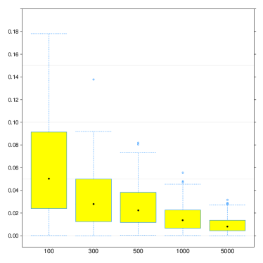
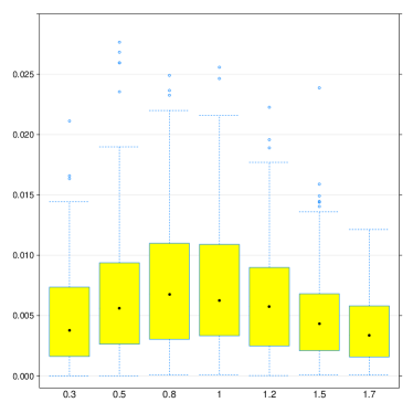
Figure 1: Left: boxplots of the distance $|\hat{f}_{h_{\star}}(1)-f_{X}(1)|$, where the estimate $\hat{f}_{h_{\star}}(1)$ is based on $n\in\{100,300,500,1000,5000\}$ observations of the r.v. $Y$ under uniformly distributed errors. Right: boxplots of the distance $|\hat{f}_{h_{\star}}(x)-f_{X}(x)|$ for $x\in\{0.3,0.5,0.8,1.0,1.2,1.5,1.7\},$ where the estimate $\hat{f}_{h_{\star}}(x)$ is based on $n=500$ observations of the r.v. $Y$ under uniformly distributed errors. The bandwidth $h_{\star}$ is precomputed using $300$ independent runs.

5.2 Estimation at zero

Now we illustrate behavior of the developed estimator for the case $x_{0}=0$. We consider again beta–distributed errors as in (5.1) and (5.2). Let $w(x)=e^{-x}$, and let $K$ be given by (5.3). Using the fact that $\widetilde{w}(z)=\Gamma(z)$, we have for any $s>\max(0,\nu)$

$$\frac{1}{2\pi}\int_{-\infty}^{\infty}e^{-i\omega y}\frac{\widetilde{w}(s+i\omega)}{\widetilde{g}(1-s-i\omega)}\mathrm{d}\omega=\frac{1}{2\pi}\int_{-\infty}^{\infty}e^{-i\omega y}\Gamma(s+i\omega)\Big{(}1-\frac{s+i\omega}{\nu}\Big{)}\mathrm{d}\omega$$

$$=\frac{1}{2\pi}\int_{-\infty}^{\infty}e^{-i\omega y}\Gamma(s+i\omega)\mathrm{d}\omega-\frac{1}{2\pi\nu}\int_{-\infty}^{\infty}e^{-i\omega y}\Gamma(1+s+i\omega)\mathrm{d}\omega.$$

The well-known identity

$$\frac{1}{2\pi}\int_{-\infty}^{\infty}e^{-i\omega y}\Gamma(s+i\omega)\,\mathrm{d}\omega=e^{sy}\exp\left(-e^{y}\right),\quad y\in\mathbb{R}$$

leads to

$$\frac{1}{2\pi}\int_{-\infty}^{\infty}e^{-i\omega y}\left(1-\frac{s+i\omega}{\nu}\right)\Gamma(s+i\omega)\,\mathrm{d}\omega =e^{sy}\exp\left(-e^{y}\right)\left(1-\frac{e^{y}}{\nu}\right).$$

Then using (4.4) and a straightforward algebra, we obtain

$$L_{s,h}(y)=\sum_{j=1}^{m+1}\tbinom{m+1}{j}(-1)^{j+1}\frac{1}{jh}\exp\Big{\{}-\frac{y}{jh}\Big{\}}\Big{(}1-\frac{y}{jh\nu}\Big{)}.$$

The corresponding estimator is $\hat{f}_{h}(0):=\frac{1}{n}\sum_{i=1}^{n}L_{s,h}(Y_{i})$.

In our simulation study we take $f_{X}(x)=2\exp(-2x)$ so that $f_{X}(0)=2$ and the distribution of $\eta$ as in (5.1) with $\nu\in\{1,\frac{1}{2}\}$. In Figure 2 we present box plots of the quantity $|\hat{f}_{h}(0)-f_{X}(0)|$ over $200$ simulation runs, where in each run we construct the estimate $\hat{f}_{h_{\star}}(0)$ using a precomputed bandwidth $h_{\star}$. The latter is found by minimizing $\mathbb{E}_{N}[|\hat{f}_{h_{\star}}(0)-f_{X}(0)|^{2}]$ over $h$ with empirical expectation $\mathbb{E}_{N}$ computed using $N=300$ independent simulation runs. As expected, in the case $\nu=1$ the estimator is more accurate than in the case $\nu=1/2$.

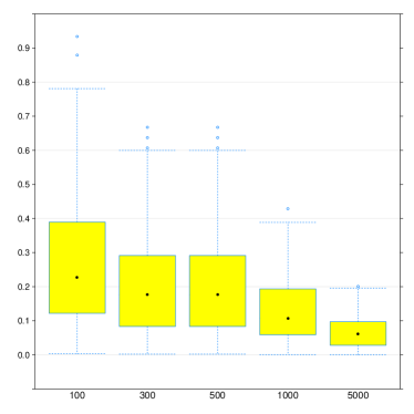
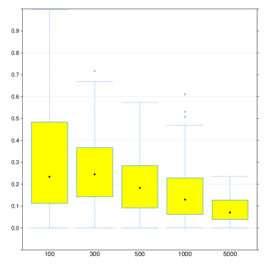
Figure 2: Boxplots of the distance $|\hat{f}_{h}(0)-f_{X}(0)|$, where the estimate $\hat{f}_{h}(0)$ is based on $n\in\{100,300,500,1000,5000\}$ observations of the r.v. $Y$ under beta-distributed errors with density (5.1) with parameters $\nu=1$ (left) and $\nu=1/2$ (right).

6 Proofs of main results

In the proofs below $c_{0},c_{1},c_{2},\ldots$ denote positive constants depending on the parameters appearing in Assumptions [G1]–[G5] and on $\beta$ only unless specified otherwise.

6.1 Proof of Theorem 1

Note that under Assumption [G1] condition (3.15) with $q>\gamma+1$ guarantees that the estimator $\hat{f}_{h}(x_{0})=\hat{f}_{0,h}(x_{0})$ is well–defined. Indeed, under this condition $\widehat{K}(\cdot h)/\widetilde{g}(1-i\cdot)\in{\mathbb{L}}_{1}({\mathbb{R}})\cap{\mathbb{L}}_{2}({\mathbb{R}})$.

1⁰. The next statement establishes an upper bound on the bias of $\hat{f}_{s,h}(x_{0})$.

Lemma 3.

Let $K_{h}(\cdot,\cdot)$ be given by (3.2), where $K$ satisfies (3.14) with $m\geq\lfloor\beta\rfloor+1$; then for any $x>0$ and $h\in(0,\ln r)$

$$\sup_{f\in{\mathscr{H}}_{x,r}(A,\beta)}\Big{|}\int_{-\infty}^{\infty}K_{h}(x,y)f(y)\mathrm{d}y-f(x)\Big{|}\leq c_{0}A\|K\|_{1}\Big{[}h^{\beta}|x|^{\beta}+h^{\ell+1}\sum_{k=0}^{\ell}|x|^{k}\Big{]},$$

where $c_{0}$ depends on $\beta$ only, and $\|K\|_{1}=\int_{-1}^{1}|K(x)|\mathrm{d}x$.

The proof of Lemma 3 is given in Section 7.

2⁰. Now we derive an upper bound on the variance. Using the Cauchy–Schwarz inequality we obtain

$$\mathbb{E}_{f_{X}}\big{[}L_{h}^{2}(x_{0},Y_{j})\big{]}\\ =\frac{1}{4\pi^{2}x_{0}^{2}}\int_{-\infty}^{\infty}\int_{-\infty}^{\infty}|x_{0}|^{i(\omega-\mu)}\widetilde{f}_{Y}(1-i(\omega-\mu))\frac{\widehat{K}(\omega h)}{\widetilde{g}(1-i\omega)}\cdot\overline{\frac{\widehat{K}(\mu h)}{\widetilde{g}(1-i\mu)}}\mathrm{d}\omega\mathrm{d}\mu\\[5.69054pt] \leq\;\frac{1}{4\pi^{2}x_{0}^{2}}\int_{-\infty}^{\infty}|\widetilde{f}_{Y}(1-i\mu)|\mathrm{d}\mu\int_{-\infty}^{\infty}\frac{|\widehat{K}(\omega h)|^{2}}{|\widetilde{g}(1-i\omega)|^{2}}\mathrm{d}\omega.$$

If $\gamma>1$ then $\widetilde{f}_{Y}(1-i\mu)$ is integrable:

$$\int_{-\infty}^{\infty}|\widetilde{f}_{Y}(1-i\mu)|\mathrm{d}\mu=\int_{-\infty}^{\infty}|\widetilde{f}_{X}(1-i\mu)|\cdot|\widetilde{g}(1-i\mu)|\mathrm{d}\mu\\ \leq\int_{-\infty}^{\infty}|\widetilde{g}(1-i\mu)|\mathrm{d}\mu\leq c_{1}<\infty,$$

where the upper bound in (3.13) has been used. Moreover, in view of (3.15) and the lower bound in (3.13) we have

$$\int_{-\infty}^{\infty}\frac{|\widehat{K}(\omega h)|^{2}}{|\widetilde{g}(1-i\omega)|^{2}}\mathrm{d}\omega\;\leq\;c_{2}h^{-2\gamma-1}.$$

Combining these bounds we obtain ${\rm var}_{f_{X}}\{\hat{f}_{h}(x_{0})\}\leq c_{3}x_{0}^{-2}h^{-2\gamma-1}n^{-1}$.

On the other hand, Lemma 3 and $h\leq 1$ imply that

$$\sup_{f_{X}\in{\mathscr{H}}_{x_{0},r}(A,\beta)}\big{|}\mathbb{E}_{f_{X}}[\hat{f}_{h}(x_{0})]-f_{X}(x_{0})\big{|}\leq c_{3}A(x_{0}^{\beta}+1)h^{\beta}.$$

Then (3.17) follows from substitution of $h_{*}$ in the bounds for the bias and the variance.    

6.2 Proof of Theorem 2

The proof is based on the standard technique for proving lower bounds (see [17, Chapter 2]). Recall that for two generic functions $u$ and $w$ on $[0,\infty)$ we write $[w\star u](y):=\int_{0}^{\infty}(1/x)w(x)u(y/x)\mathrm{d}x$.

0⁰. Let $\psi:{\mathbb{R}}\to{\mathbb{R}}$ be a function such that its Fourier transform $\widehat{\psi}$ is an infinitely differentiable function satisfying for some $\delta\in(0,\tfrac{1}{4})$

$${\cal F}[\psi;\omega]=\widehat{\psi}(\omega)=\left\{\begin{array}[]{ll}1,&\omega\in[-2+\delta,-1-\delta]\cup[1+\delta,2-\delta],\\ 0,&\omega\in(-\infty,-2]\cup[-1,1]\cup[2,\infty).\end{array}\right.$$

Let $x_{0}\geq c_{0}>0$ for some constant $c_{0}$, and define

$$f_{X}^{(0)}(x):=\frac{1}{\pi x[1+\ln^{2}(x/x_{0})]},\;\;\;x>0.$$

Define

$$f_{X}^{(1)}(x)=f_{X}^{(0)}(x)+\theta\psi_{h}(x),\;\;\;\;\psi_{h}(x):=\frac{1}{x}\psi\bigg{(}\frac{\ln(x/x_{0})}{h}\bigg{)},$$

where $h\in(0,1)$ and $\theta>0$ are the parameters to be specified.

1⁰. First we show that if $\theta$ is small enough, $\theta\leq\min\{\tfrac{1}{2},c_{1}h^{-2}\}$ then $f_{X}^{(1)}$ is a probability density on $[0,\infty)$. Indeed, since $\widehat{\psi}(0)=0$

$$\int_{0}^{\infty}\psi_{h}(x)\mathrm{d}x=\int_{0}^{\infty}\frac{1}{x}\psi\bigg{(}\frac{\ln(x/x_{0})}{h}\bigg{)}\mathrm{d}x=h\int_{-\infty}^{\infty}\psi(t)\mathrm{d}t=0.$$

Thus, $f_{X}^{(1)}$ integrates to one. Moreover, by construction $\psi$ is rapidly decreasing as $t\to\infty$; in particular, $|\psi(t)|\leq\pi^{-1}\min\{1,c_{1}t^{-2}\}$, $\forall t\in{\mathbb{R}}$ with some absolute constant $c_{1}$. Therefore, the conditions $\theta\leq\frac{1}{2}$ and $c_{1}\theta h^{2}\leq\frac{1}{2}$ imply that $\theta|\psi(t/h)|\leq[\pi(1+t^{2})]^{-1}$, which, in turn shows that $f_{X}^{(1)}$ is non–negative. Therefore $f_{X}^{(1)}$ is the probability density.

2⁰. First we note that if $x_{0}\geq c_{0}>0$ for some $c_{0}$ large enough then $f_{X}^{(0)}\in{\mathscr{H}}_{x_{0},r}(A/2,\beta)$. Now we show that if $\theta=c_{2}Ax_{0}^{\beta+1}h^{\beta}$ for some constant $c_{2}$ then $f_{X}^{(1)}\in{\mathscr{H}}_{x_{0},r}(A,\beta)$.

For simplicity and without loss of generality assume that $\beta$ is integer, $\beta\geq 1$. Then by the Faá di Bruno formula

$$\psi_{h}^{(\beta)}(x)=\sum_{j=0}^{\beta}\binom{\beta}{j}\frac{(-1)^{j}}{x^{j+1}}\frac{d^{\beta-j}}{dx^{\beta-j}}\psi\bigg{(}\frac{\ln(x/x_{0})}{h}\bigg{)}\\ =\sum_{j=0}^{\beta}\binom{\beta}{j}\frac{(-1)^{j}}{x^{j+1}}\sum\frac{(\beta-j)!}{k_{1}!\cdots k_{\beta-j}!}\psi^{(k)}\bigg{(}\frac{\ln(x/x_{0})}{h}\bigg{)}h^{-k}x^{-(\beta-j)}\prod_{i=1}^{\beta-j}\bigg{[}\frac{(-1)^{i+1}}{i!}\bigg{]}^{k_{i}},$$

where the second summation is over all partitions of $\beta-j$, and $k:=k_{1}+\ldots+k_{\beta-j}$, $k_{1}+2k_{2}+\cdots+(\beta-j)k_{\beta-j}=\beta-j$. It follows from this expression and the fact that $h<1$ that

$$|\psi_{h}^{(\beta)}(x)|\leq c_{3}x^{-\beta-1}h^{-\beta}\max_{k=1,\ldots,\beta}\bigg{|}\psi^{(k)}\bigg{(}\frac{\ln(x/x_{0})}{h}\bigg{)}\bigg{|},\;\;\;\forall x>0,$$

where $c_{3}$ depends on $\beta$ only. Since $\psi$ is an infinite differentiable rapidly decreasing function, we obtain

$$|\psi^{(\beta)}_{h}(x)|\leq c_{4}x_{0}^{-\beta-1}h^{-\beta},\;\;\;\;\;r^{-1}x_{0}\leq x\leq rx_{0},$$

where $c_{4}$ depends on $\beta$. Then setting $\theta=c_{2}Ax_{0}^{\beta+1}h^{\beta}$, by choice of $c_{2}$ we obtain $f_{X}^{(1)}\in{\mathscr{H}}_{x_{0},r}(A,\beta)$.

3⁰. Next we bound the $\chi^{2}$–divergence between $f^{(1)}_{Y}$ and $f^{(0)}_{Y}$. We have

$$f_{Y}^{(0)}(y) = [f_{X}^{(0)}\star g](y)=\frac{1}{\pi y}\int_{0}^{\infty}\frac{g(x)}{1+[\ln(y/x_{0})-\ln(x)]^{2}}\mathrm{d}x$$

$$\geq \frac{1}{\pi y[1+2\ln^{2}(y/x_{0})]}\int_{0}^{\infty}\frac{g(x)}{1+2\ln^{2}(x)}\mathrm{d}x\geq\frac{c_{5}}{y[1+2\ln^{2}(y/x_{0})]}.$$

Furthermore,

$$f_{Y}^{(1)}(y)-f_{Y}^{(0)}(y) = \theta[g\star\psi_{h}](y)=\theta\int_{0}^{\infty}\frac{1}{x}g(x)\psi_{h}(y/x)\mathrm{d}x$$ (6.1)

$$= \frac{\theta}{2\pi y}\int_{-\infty}^{\infty}\widetilde{g}(1+i\omega)\widetilde{\psi}_{h}(1+i\omega)y^{-i\omega}\mathrm{d}\omega,$$

where in the second line we have applied the inverse Mellin transform formula. By definition of $\psi_{h}$,

$$\widetilde{\psi}_{h}(1+i\omega)=\int_{0}^{\infty}x^{i\omega}\psi_{h}(x)\mathrm{d}x=\int_{0}^{\infty}x^{i\omega-1}\psi\bigg{(}\frac{\ln(x/x_{0})}{h}\bigg{)}\mathrm{d}x\\ =hx_{0}^{i\omega}\int_{-\infty}^{\infty}e^{ith\omega}\psi(t)\mathrm{d}t=hx_{0}^{i\omega}\widehat{\psi}(-\omega h).$$

Substituting this expression in (6.1) we obtain

$$f_{Y}^{(1)}(y)-f_{Y}^{(0)}(y)=\frac{\theta h}{2\pi y}\int_{-\infty}^{\infty}\widetilde{g}(1+i\omega)\widehat{\psi}(-\omega h)e^{-i\omega\ln(y/x_{0})}\mathrm{d}\omega=:\frac{\theta h}{2\pi y}\rho\big{(}\ln(y/x_{0})).$$

The $\chi^{2}$–divergence between $f_{Y}^{(1)}$ and $f_{Y}^{(0)}$ is bounded as follows

$$\chi^{2}(f_{Y}^{(1)},f_{Y}^{(0)})=\int_{0}^{\infty}\frac{(f_{Y}^{(1)}(y)-f_{Y}^{(0)}(y))^{2}}{f_{Y}^{(0)}(y)}\mathrm{d}y\\ \;\;\;\leq c_{6}\theta^{2}h^{2}\int_{0}^{\infty}[1+2\ln^{2}(y/x_{0})]\frac{1}{y}\rho^{2}\big{(}\ln(y/x_{0})\big{)}\mathrm{d}y=c_{6}\theta^{2}h^{2}\int_{-\infty}^{\infty}(1+2t^{2})\rho^{2}(t)\mathrm{d}t.$$

By Parseval’s identity, definition of $\psi$ and Assumption [G1]

$$\int_{-\infty}^{\infty}\rho^{2}(t)\mathrm{d}t=\int_{-\infty}^{\infty}|\widetilde{g}(1+i\omega)|^{2}|\widehat{\psi}(-\omega h)|^{2}\mathrm{d}\omega\leq 2\int_{1/h}^{2/h}|\widetilde{g}(1+i\omega)|^{2}\mathrm{d}\omega\leq c_{7}h^{2\gamma-1}.$$ (6.2)

Moreover, using Assumptions [G1] and [G1^′]

$$\int_{-\infty}^{\infty}t^{2}\rho^{2}(t)\mathrm{d}t=\int_{-\infty}^{\infty}\Big{|}\frac{\mathrm{d}}{\mathrm{d}\omega}\widetilde{g}(1+i\omega)\widehat{\psi}(-\omega h)\Big{|}^{2}\mathrm{d}\omega\\ \leq 2\int_{-\infty}^{\infty}|\widetilde{g}^{\prime}(1+i\omega)|^{2}|\widehat{\psi}(-\omega h)|^{2}\mathrm{d}\omega+2\int_{-\infty}^{\infty}|\widetilde{g}(1+i\omega)|^{2}|\widehat{\psi}^{\prime}(-\omega h)|^{2}h^{2}\mathrm{d}\omega\\ \leq c_{8}h^{2\gamma-1}+c_{9}h^{2\gamma+1}.$$

Combining these bounds with (6.2) for $h$ small enough we obtain

$$\chi^{2}(P^{(1)},P^{(0)})\leq c_{9}\theta^{2}h^{2\gamma+1}=c_{10}A^{2}x_{0}^{2\beta+2}h^{2\beta+2\gamma+1}.$$

4⁰. Now we complete the proof. Let

$$h=h_{*}:=c_{11}x_{0}^{-\frac{2\beta+2}{2\beta+2\gamma+1}}(A^{2}n)^{-\frac{1}{2\beta+2\gamma+1}}.$$

With this choice $\theta=c_{2}Ax_{0}^{\beta+1}h_{*}^{\beta}\leq\tfrac{1}{2}$ for $n$ large enough so $f_{X}^{(1)}\in{\mathscr{H}}_{x_{0},r}(A,\beta)$. We obtain $\chi^{2}(f_{Y}^{(1)},f_{Y}^{(0)})\leq 1/n$ so that the hypotheses $f_{X}=f^{(0)}_{X}$ and $f_{X}=f^{(1)}_{X}$ are indistinguishable from the observations $Y_{1},\ldots,Y_{n}$. Moreover, with this choice of the parameter $h$

$$\Big{|}f_{X}^{(1)}(x_{0})-f_{X}^{(0)}(x_{0})\Big{|}=\theta|\psi_{h_{*}}(x_{0})|=c_{12}Ax_{0}^{\beta+1}h_{*}^{\beta}x_{0}^{-1}|\psi(0)|\\ =c_{13}A^{\frac{2\gamma+1}{2\beta+2\gamma+1}}x_{0}^{\frac{\beta(2\gamma-1)}{2\beta+2\gamma+1}}n^{-\frac{\beta}{2\beta+2\gamma+1}}~{}.$$

This completes the proof of the theorem.    

6.3 Proof of Theorem 3

The bound on bias of $\hat{f}_{s,h}(x_{0})$ given in Lemma 3 remains intact. We consider only the variance term. For

$$L_{s,h}(x,y)=\frac{1}{2\pi x}\int_{-\infty}^{\infty}\bigg{(}\frac{x}{y}\bigg{)}^{s+i\omega}\,\frac{\widecheck{K}((s+i\omega)h)}{\widetilde{g}(1-s-i\omega)}\,\mathrm{d}\omega$$

we have

$$\mathbb{E}_{f_{X}}\big{[}L^{2}_{s,h}(x_{0},Y_{j})\big{]}\\ =\frac{1}{4\pi^{2}x_{0}^{2-2s}}\int_{-\infty}^{\infty}\int_{-\infty}^{\infty}x_{0}^{i(\omega-\mu)}\widetilde{f}_{Y}(1-2s-i(\omega-\mu))\frac{\widecheck{K}((s+i\omega)h)}{\widetilde{g}(1-s-i\omega)}\cdot\overline{\frac{\widecheck{K}((s+i\mu)h)}{\widetilde{g}(1-s-i\mu)}}\mathrm{d}\omega\mathrm{d}\mu\\[5.69054pt] \leq\frac{1}{4\pi^{2}x_{0}^{2-2s}}\int_{-\infty}^{\infty}|\widetilde{f}_{Y}(1-2s-i\mu)|\mathrm{d}\mu\int_{-\infty}^{\infty}\bigg{|}\frac{\widecheck{K}((s+i\omega)h)}{\widetilde{g}(1-s-i\omega)}\bigg{|}^{2}\mathrm{d}\omega.$$

Since $f_{X}\in{\mathscr{F}}_{\alpha,M}(A,\beta)$, $|\widetilde{f}_{X}(1-2s-i\mu)|\leq 1+M<\infty$ for all $\mu\in{\mathbb{R}}$ and $-\alpha\leq s\leq 0$. For such $s$

$$\int_{-\infty}^{\infty}|\widetilde{f}_{Y}(1-2s-i\mu)|\mathrm{d}\mu\leq(1+M)\int_{-\infty}^{\infty}|\widetilde{g}(1-2s-i\mu)|\mathrm{d}\mu\;\leq\;c_{1}(1+M),$$

provided that $a<1-2s<b$. Setting $s=s_{*}=\max\{-\alpha,\tfrac{1}{2}(1-b)+\epsilon\}$ for any $\epsilon>0$ we obtain

$$\mathbb{E}_{f_{X}}\big{[}L^{2}_{s_{*},h}(x_{0},Y_{j})\big{]}\leq\frac{c_{2}(1+M)}{4\pi^{2}x_{0}^{2-2s_{*}}}\int_{-\infty}^{\infty}\bigg{|}\frac{\widecheck{K}((s_{*}+i\omega)h)}{\widetilde{g}(1-s_{*}-i\omega)}\bigg{|}^{2}\mathrm{d}\omega.$$ (6.3)

Furthermore,

$$\widecheck{K}((s_{*}+i\omega)h)=\int_{-1}^{1}K(x)e^{-s_{*}hx}e^{-i\omega hx}\mathrm{d}x={\cal F}[v_{s_{*},h};\omega h]=\widehat{v}_{s_{*},h}(\omega h),$$

where $v_{s,h}(x):=K(x)e^{-shx}{\bf 1}_{[-1,1]}(x)$. Therefore

$$\int_{-\infty}^{\infty}\bigg{|}\frac{\widecheck{K}((s_{*}+i\omega)h)}{\widetilde{g}(1-s_{*}-i\omega)}\bigg{|}^{2}\mathrm{d}\omega=\int_{-\infty}^{\infty}\bigg{|}\frac{\widehat{v}_{s_{*},h}(-\omega h)}{\widetilde{g}(1-s_{*}-i\omega)}\bigg{|}^{2}\mathrm{d}\omega\\ \leq\frac{c_{3}}{h^{2\gamma+1}}\int_{-\infty}^{\infty}|\widehat{v}_{s_{*},h}(\omega)|^{2}(1+|\omega|^{2\gamma})\mathrm{d}\omega,$$ (6.4)

where $c_{3}$ may depend on $s_{*}$. In view of (3.15), $v_{s,h}$ is $q$ times continuously differentiable on its support, and $v_{s,h}^{(q)}(x)=\sum_{j=0}^{q}\tbinom{q}{j}K^{(j)}(x)(-sh)^{q-j}e^{-shx}$. Therefore

$$\big{\|}v_{s_{*},h}^{(q)}\big{\|}_{2}\leq\sum_{j=0}^{q}\tbinom{q}{j}e^{2|s_{*}|h}|s_{*}h|^{q-j}\bigg{[}\int_{-1}^{1}|K^{(j)}(x)|^{2}\mathrm{d}x\bigg{]}^{1/2}\\ \leq c_{4}\max_{j=0,\ldots,q}\|K^{(j)}\|_{2}\;\leq\;c_{5}C_{K}.$$

Taking into account that $q>\gamma+1$ and combining this inequality with (6.4) and (6.3) we obtain

$${\rm var}_{f_{X}}\big{\{}\hat{f}_{s_{*},h}(x_{0})\}\leq c_{6}(1+M)x_{0}^{-2+2s_{*}}h^{-2\gamma-1}n^{-1}.$$

This bound together with the bound on the bias leads to the announced result.

   

6.4 Proof of Theorem 4

The proof goes along the same lines as the proof of Theorem 1. In the proof below $c_{1},c_{2},\ldots$ stand for positive constants depending on $\beta$ and $\lambda$ only.

It is immediate to verify that

$$|\widehat{K}(\omega)|\leq c_{1}\exp\{-\omega^{2\lambda}/2\lambda\},\;\;\;\forall\omega\in{\mathbb{R}}.$$ (6.5)

This fact together with Assumption [G2] guarantees that the estimator $\hat{f}_{h_{*}}(x_{0})$ is well–defined. In addition, by [11, Chapter IV, § 7] as $|t|\to\infty$

$$w(t)=2\sqrt{\tfrac{1}{2\lambda-1}}|t|^{-(\lambda-1)/(2\lambda-1)}\exp\Big{\{}-\Big{(}\tfrac{2\lambda-1}{2\lambda}\Big{)}\sin\Big{(}\tfrac{\pi}{2(2\lambda-1)}\Big{)}|t|^{2\lambda/(2\lambda-1)}\Big{\}}\\[5.69054pt] \times\Big{[}\cos\bigg{(}\tfrac{2\lambda-1}{2\lambda}|t|^{2\lambda/(2\lambda-1)}\cos\Big{(}\frac{\pi}{2(2\lambda-1)}\Big{)}\bigg{)}+O\Big{(}|t|^{-2\lambda/(2\lambda-1)}\Big{)}\Big{]}.$$

Therefore, it follows from (3.26) that for large $|t|$ one has

$$|K(t)|\leq c_{2}|t|^{-(\lambda-1)/(2\lambda-1)}\;\exp\Big{\{}-c_{3}|t|^{2\lambda/(2\lambda-1)}\Big{\}}.$$ (6.6)

First we bound the bias of the estimator $\hat{f}_{h_{*}}(x_{0})$. To that end we note that the proof of Lemma 3 applies verbatim; the only difference is that now the integration in (7.12) is over the whole real line because $K$ is not compactly supported. However, since $K$ is a bounded function and in view of (6.6) we have

$$\int_{-\infty}^{\infty}|t|^{\ell+1}e^{\ell|th|}|K(t)|\mathrm{d}t\leq\int_{-\infty}^{\infty}|t|^{\ell+\frac{\lambda}{2\lambda-1}}\exp\Big{\{}\ell|t|-c_{3}|t|^{-\frac{2\lambda}{2\lambda-1}}\Big{\}}\mathrm{d}t\leq c_{4}.$$

This inequality and reasoning of the proof of Lemma 3 yield

$$\sup_{f\in{\mathscr{H}}_{x,r}(A,\beta)}\Big{|}\int_{-\infty}^{\infty}K_{h}(x,y)f(y)\mathrm{d}y-f(x)\Big{|}\leq c_{5}A\Big{[}h^{\beta}|x|^{\beta}+h^{\ell+1}\sum_{k=0}^{\ell}|x|^{k}\Big{]}.$$

To bound the variance we follow the lines of the proof of Theorem 1. In particular, in view of (6.5) and Assumption [G2] by straightforward algebra we have for small enough $h$

$$\mathbb{E}_{f_{X}}\big{[}L_{h}^{2}(x_{0},Y_{j})\big{]}\leq\frac{c_{6}}{x_{0}^{2}}\int_{-\infty}^{\infty}\frac{|\widehat{K}(\omega h)|^{2}}{|\widetilde{g}(1-i\omega)|^{2}}\mathrm{d}\omega\\ \leq\frac{c_{7}}{x_{0}^{2}}\bigg{\{}1+\int_{\omega_{0}\leq|\omega|\leq\omega_{1}}+\int_{|\omega|>\omega_{1}}|\omega|^{-2\nu}\exp\{|\omega|\gamma-|\omega h|^{2\lambda}/\lambda\}\mathrm{d}\omega\bigg{\}}\\ \leq\frac{c_{8}}{x_{0}^{2}}\exp\Big{\{}c_{9}\big{(}\gamma h^{-1}\big{)}^{2\lambda/(2\lambda-1)}\Big{\}},$$

where we set $\omega_{1}:=(\lambda\gamma)^{1/(2\lambda-1)}h^{-2\lambda/(2\lambda-1)}$. Then the result of the theorem follows from balancing the bounds in the two previous display formulas.    

6.5 Proof of Theorem 5

In the proof below $c_{1},c_{2},\ldots$ stand for positive constants; they can depend on parameters appearing in assumptions [G3] and [G4] and on parameter $\beta$ only. The proof proceeds in steps.

1⁰. First we show that under the premise of the theorem the estimator $\hat{f}_{s_{*},h}(0)$ is well defined. It follows from the definition of function $\psi_{s}(x)$ that

$$\widetilde{\psi}_{s}(s+i\omega)=\frac{1}{\sqrt{2\pi}}e^{-\frac{1}{2}(1-s)^{2}}\int_{0}^{\infty}x^{s+i\omega-1}x^{-s}\exp\{-\tfrac{1}{2}[\ln x]^{2}\}\mathrm{d}x\\ =\frac{1}{\sqrt{2\pi}}e^{-\frac{1}{2}(1-s)^{2}}e^{-\frac{1}{2}\omega^{2}};$$

therefore

$$\int_{0}^{\infty}\psi_{s}\Big{(}\frac{x}{j}\Big{)}x^{s+i\omega-1}\mathrm{d}x=j^{s+i\omega}\widetilde{\psi}_{s}(s+i\omega)=\frac{j^{s+i\omega}}{\sqrt{2\pi}}e^{-\frac{1}{2}(1-s)^{2}}e^{-\frac{1}{2}\omega^{2}},$$

and

$$\widetilde{K}_{s}(s+i\omega)=\frac{1}{\sqrt{2\pi}}e^{-\frac{1}{2}(1-s)^{2}}e^{-\omega^{2}/2}\sum_{j=1}^{m+1}\tbinom{m+1}{j}(-1)^{j+1}j^{s-1+i\omega}.$$

The last expression implies that

$$|\widetilde{K}_{s}(s+i\omega)|\leq c_{1}m^{s}e^{-\frac{1}{2}(1-s)^{2}}e^{-\omega^{2}/2},$$ (6.7)

where $c_{1}$ depends on $m$ only. Next we observe that Assumption [G3] implies $1-s_{*}=1-\frac{1}{2}(1-p)\in\Omega_{g}$, so that $\widetilde{g}(1-s_{*}+i\omega)$ is well defined. Then in view of (6.7) and condition (4.8) of Assumption [G4], $\widetilde{K}_{s_{*}}(s_{*}+i\cdot)/\widetilde{g}(1-s_{*}-i\cdot)\in{\mathbb{L}}_{1}({\mathbb{R}})\cap{\mathbb{L}}_{2}({\mathbb{R}})$ so that $\hat{f}_{s_{*},h}(0)$ is well defined.

2⁰. Our next step is to prove the following statement about local behavior of the density $f_{Y}$ near the origin. This result is instrumental in establishing an upper bound on the variance term.

Lemma 4.

Let Assumption [G3] hold, and assume that $f_{X}(t)\leq M$, $\forall t$.

• If $p=0$ then for all $y\leq\delta$

  $$f_{Y}(y)\leq C_{1}(1+M)|\ln y|^{q+1}+M\delta^{-1},$$

  where $C_{1}$ depends on $q$ only.

• If $p\in(0,1)$ then for all $y\leq\delta$

  $$f_{Y}(y)\leq C_{2}\big{(}1+Mp^{-1}\big{)}y^{-p}|\ln y|^{q}+M\delta^{-1},$$

  where $C_{2}$ depends on $q$ only.

The proof of the lemma is given in Section 7.

3⁰. Now we are ready to establish an upper bound on the variance term. Define

$$\rho_{s}(x):=\frac{1}{2\pi}\int_{-\infty}^{\infty}e^{-i\omega x}\frac{\widetilde{K}_{s}(s+i\omega)}{\widetilde{g}(1-s-i\omega)}\mathrm{d}\omega.$$

With this notation $L_{s,h}(y)=h^{s-1}y^{-s}\rho_{s}(\ln(y/h))$ [cf. (4.4)], and therefore

$$\mathbb{E}_{f_{X}}\big{[}L^{2}_{s,h}(Y)\big{]}=\frac{1}{h^{2-2s}}\int_{0}^{\infty}\frac{\rho_{s}^{2}(\ln(y/h))}{y^{2s}}f_{Y}(y)\mathrm{d}y.$$

Now we bound the last integral which can be written as a sum $J_{1}+J_{2}$, where

$$J_{1}:=\frac{1}{h^{2-2s}}\int_{0}^{\delta}\frac{\rho_{s}^{2}(\ln(y/h))}{y^{2s}}f_{Y}(y)\mathrm{d}y,\;J_{2}:=\frac{1}{h^{2-2s}}\int_{\delta}^{\infty}\frac{\rho_{s}^{2}(\ln(y/h))}{y^{2s}}f_{Y}(y)\mathrm{d}y.$$

Using Lemma 4 for $p=0$ and $s=s_{*}=\frac{1}{2}$ by straightforward algebra we obtain

$$J_{1} \leq \frac{c_{1}M}{h}\int_{0}^{\delta}y^{-1}\rho_{s_{*}}(\ln(y/h))\big{[}|\ln y|^{q+1}+\delta^{-1}\big{]}\mathrm{d}y$$

$$\leq \frac{c_{2}M}{h}\bigg{(}|\ln h|^{q+1}\int_{-\infty}^{\infty}\rho_{s_{*}}^{2}(t)\mathrm{d}t+\int_{-\infty}^{\infty}\rho_{s_{*}}^{2}(t)|t|^{q+1}\mathrm{d}t\bigg{)}\leq c_{3}Mh^{-1}|\ln h|^{q+1},$$

where the last inequality follows from condition [G4] [cf. (4.8) and (4.9)]. If $p\in(0,1)$ then using Lemma 4 for $s=s_{*}=\frac{1}{2}(1-p)$ we have similarly

$$J_{1} \leq \frac{c_{4}M}{h^{2-2s_{*}}}\int_{0}^{\delta_{0}}\frac{1}{y}\rho_{s_{*}}^{2}(\ln(y/h))\frac{y^{-p}|\ln y|^{q+\varkappa}}{y^{2s_{*}-1}}\mathrm{d}y$$

$$\leq \frac{c_{5}M}{h^{1+p}}\bigg{(}|\ln h|^{q}\int_{-\infty}^{\infty}\rho_{s_{*}}^{2}(t)\mathrm{d}t+\int_{-\infty}^{\infty}\rho_{s_{*}}^{2}(t)|t|^{q}\mathrm{d}t\bigg{)}\leq c_{6}Mh^{-1-p}[\ln(1/h)]^{q}.$$

Combining the last two upper bounds on $J_{1}$ in cases $p=0$ and $p\in(0,1)$ we can write

$$J_{1}\leq c_{7}Mh^{-1-p}[\ln(1/h)]^{q+\varkappa},$$

where $\varkappa$ is defined in (4.10).

In order to bound $J_{2}$ we note that (4.8) implies $|\rho_{s_{*}}(x)|\leq c_{8}<\infty$, $\forall x$; therefore

$$J_{2}\leq c_{8}^{2}h^{-1-p}\int_{\delta_{0}}^{\infty}y^{p-1}f_{Y}(y)\mathrm{d}y\leq c_{9}h^{-1-p}.$$

Combining the bounds on $J_{1}$ and $J_{2}$ we obtain

$$\mathbb{E}_{f_{X}}\big{[}L^{2}_{{s_{*}},h}(Y)\big{]}\leq c_{10}Mh^{-1-p}[\ln(1/h)]^{q+\varkappa}.$$

4⁰. We proceed with bounding the bias of $\hat{f}_{s_{*},h}(0)$. By construction of $K_{s_{*},h}(x)$ we have

$$\int_{0}^{\infty}(1/h)K_{s_{*}}(x/h)[f_{X}(x)-f_{X}(0)]\mathrm{d}x=\int_{0}^{\infty}K_{s_{*}}(u)[f_{X}(uh)-f_{X}(0)]\mathrm{d}x$$

$$=\int_{0}^{r/h}K_{s_{*}}(u)\Big{[}\sum_{j=1}^{\ell-1}\frac{1}{j!}f_{X}^{(j)}(0)(uh)^{j}+\frac{1}{\ell!}f_{X}^{(\ell)}(\xi uh)(uh)^{\ell}\Big{]}\mathrm{d}u$$

$$+\int_{r/h}^{\infty}K_{s_{*}}(u)[f_{X}(uh)-f_{X}(0)]\mathrm{d}u.$$

Since $f_{X}(x)\leq M$, $\forall x$, by (4.2) and (4.3)

$$\bigg{|}\int_{r/h}^{\infty}K_{s_{*}}[f_{X}(uh)-f_{X}(0)]\mathrm{d}u\bigg{|}\leq 2M\sum_{j=1}^{m+1}\tbinom{m+1}{j}\int_{r/h}^{\infty}\psi_{s_{*}}(x)\mathrm{d}x\\ \leq c_{1}M\exp\{-c_{2}[\ln(r/h)]^{2}\}.$$

Furthermore, it is readily verified that for small enough $h$

$$\bigg{|}\int_{0}^{r/h}K_{s_{*}}(u)u^{j}\mathrm{d}u\bigg{|}=\bigg{|}\int_{r/h}^{\infty}K_{s_{*}}(u)u^{j}\mathrm{d}u\bigg{|}\leq c_{3}\exp\big{\{}-c_{4}[\ln\big{(}\tfrac{r}{mh}\big{)}]^{2}\big{\}}.$$

Using these facts we finally obtain that

$$\bigg{|}\int_{0}^{\infty}(1/h)K_{s_{*}}(x/h)[f_{X}(x)-f_{X}(0)]\mathrm{d}x\bigg{|}\\ \leq c_{5}Ah^{\beta}+c_{6}(1+M)\exp\big{\{}-c_{7}\big{[}\ln\big{(}\tfrac{r}{mh}\big{)}\big{]}^{2}\big{\}}.$$

We complete the proof by noting that the choice $h=h_{*}$ indicated in the statement of the theorem provides a balance for the bounds on the bias and on the variance.    

6.6 Proof of Theorem 6

The proof is based on the standard technique for proving lower bounds (see [17, Chapter 2]). Throughout the proof constants $c_{0},c_{1},\ldots$ may depend only on $\beta$ and parameters appearing in Assumptions [G3] and [G5].

1⁰. Let $M_{0}=\pi M/4$, and without loss of generality assume that $M_{0}\geq 1$. Let

$$f_{X}^{(0)}(x):=\frac{2M_{0}}{\pi(1+M_{0}x)(1+\ln^{2}(1+M_{0}x))},\quad x\geq 0.$$

It is evident that $f_{X}^{(0)}(x)\leq M/2$, $\forall x$ and $f_{X}^{(0)}\in\bar{{\mathscr{H}}}_{r}(A,\beta,M)$ provided that $A$ is large enough.

For $h>0$ define

$$f_{X}^{(1)}(x)=f_{X}^{(0)}(x)+c_{0}Ah^{\beta}\varphi\left(x/h\right),\;\;\;\varphi(x):=(1-x)e^{-x},\;\;\;x\geq 0.$$

In what follows parameter $h$ will be chosen going to zero as $n\to\infty$; in the subsequent proof we use this fact. It is evident that function $f_{X}^{(1)}$ is a probability density, and under appropriate choice of constant $c_{0}$ and for $h$ small enough it belongs to $\bar{{\mathscr{H}}}_{r}(A,\beta,M)$. We note also that

$$\widetilde{\varphi}(z)=\int_{0}^{\infty}x^{z-1}\varphi(x)\mathrm{d}x=\Gamma(z)-\Gamma(z+1),\;\;z\in\Omega_{\varphi}=\{z:{\rm Re}(z)>0\}.$$ (6.8)

Our current goal is to bound the $\chi^{2}$–divergence between the corresponding densities of observations $f_{Y}^{(0)}$ and $f_{Y}^{(1)}$. For any $s$ such that $\{z:{\rm Re}(z)=s\}\subseteq\Omega_{g}\cap\Omega_{\varphi}$ we have

$$f_{Y}^{(1)}(y)- f_{Y}^{(0)}(y)=c_{0}Ah^{\beta}\int_{0}^{\infty}\frac{1}{x}\varphi\Big{(}\frac{y}{hx}\Big{)}g(x)\mathrm{d}x$$

$$=\frac{c_{0}Ah^{\beta}}{2\pi i}\int_{s-i\infty}^{s+i\infty}\Big{(}\frac{h}{y}\Big{)}^{z}\widetilde{\varphi}(z)\widetilde{g}(z)\mathrm{d}z$$

$$=\frac{c_{0}Ah^{\beta+s}}{2\pi y^{s}}\int_{-\infty}^{\infty}\Big{(}\frac{h}{y}\Big{)}^{i\omega}\widetilde{\varphi}(s+i\omega)\widetilde{g}(s+i\omega)\mathrm{d}\omega=c_{0}Ah^{\beta+s}y^{-s}\rho_{s}(\ln(y/h)),$$

where we have used the Mellin transform inversion formula, and we have denoted

$$\rho_{s}(t):=\frac{1}{2\pi}\int_{-\infty}^{\infty}e^{-i\omega t}\widetilde{\varphi}(s+i\omega)\widetilde{g}(s+i\omega)\mathrm{d}\omega=\frac{e^{st}}{2\pi}\int_{s-i\infty}^{s+i\infty}e^{-zt}\widetilde{\varphi}(z)\widetilde{g}(z)\mathrm{d}z.$$ (6.9)

Thus

$$\chi^{2}(f_{Y}^{(0)},f_{Y}^{(1)})=c_{0}^{2}A^{2}h^{2(\beta+s)}\int_{0}^{\infty}\frac{y^{-1}\rho_{s}^{2}(\ln(y/h))}{y^{2s-1}f_{Y}^{(0)}(y)}\mathrm{d}y,$$ (6.10)

and now we will bound the integral on the right hand side under a particular choice of parameter $s$.

2⁰. Let $s=s_{*}:=\frac{1}{2}(p+1)$. Note that by the upper bound in (4.6) and by definition of $s_{*}$

$$|\widetilde{g}(s_{*}+i\omega)|\leq\int_{0}^{\infty}x^{s_{*}-1}g(x)\mathrm{d}x=\int_{0}^{\infty}x^{(p-1)/2}g(x)\mathrm{d}x\leq c_{1};$$

thus $\{z:{\rm Re}(z)=s_{*}\}\subseteq\Omega_{g}$. Let $\nu:=\frac{1}{2}(1-p)+\epsilon$, where $\epsilon$ is given in Assumption [G5]. Then $s_{*}+\nu=1+\epsilon$, and according to Assumptions [G3] and [G5], function $e^{-zt}\widetilde{g}(z)\widetilde{\varphi}(z)$ is analytic in $\{z:s_{*}\leq{\rm Re}(z)\leq s_{*}+\nu\}$. Therefore the line of integration in the last integral on the right hand side of (6.9) can be replaced by $\{z:{\rm Re}(z)=s_{*}+\nu\}$. This yields

$$\rho_{s_{*}}(t) = \frac{e^{s_{*}t}}{2\pi}\int_{s_{*}+\nu-i\infty}^{s_{*}+\nu+i\infty}e^{-zt}\widetilde{g}(z)\widetilde{\varphi}(z)\mathrm{d}z$$

$$= \frac{e^{-\nu t}}{2\pi}\int_{-\infty}^{\infty}e^{-i\omega t}\widetilde{g}(1+\epsilon+i\omega)\widetilde{\varphi}(1+\epsilon+i\omega)\mathrm{d}\omega.$$

Then it follows from Assumption [G5] that

$$|\rho_{s_{*}}(t)|\leq c_{2}e^{-\nu t}\int_{-\infty}^{\infty}|\widetilde{\varphi}(1+\epsilon+i\omega)|\mathrm{d}\omega\leq c_{3}e^{-\nu t},$$ (6.11)

where the last inequality follows from (6.8) and bounds on the Gamma function as presented in (3.24) in Example 4.

3⁰. Now we derive lower bounds on $f_{Y}^{(0)}(y)$. Note that $f_{X}^{(0)}(x)=M_{0}\bar{f}_{X}^{(0)}(M_{0}x)$ where

$$\bar{f}_{X}^{(0)}(x):=\frac{2}{\pi(1+x)(1+\ln^{2}(1+x))},\quad x\geq 0.$$

Therefore $f_{Y}^{(0)}(y)=M_{0}\bar{f}_{Y}^{(0)}(M_{0}y)$, $\bar{f}_{Y}^{(0)}(y):=[\bar{f}_{X}^{(0)}\star g](y)$ and the lower bounds on $f_{Y}^{(0)}(y)$ can be obtained in an evident way from the corresponding bounds on $\bar{f}_{Y}^{(0)}(y)$.

First we note that the lower bound in (4.6) and the arguments as in the proof of (7.16) in Lemma 4, yield for all $y<\delta/2$

$$\int_{y}^{\delta}[g(t)/t]\mathrm{d}t\geq c_{4}y^{-p}|\ln y|^{q+\varkappa},$$ (6.12)

where $\varkappa$ is defined in (4.10). In view of (6.12) for $y<\delta/2$

$$\bar{f}_{Y}^{(0)}(y) \geq \int_{y}^{\delta}\frac{2g(x)}{\pi x(1+y/x)(1+\ln^{2}(1+y/x))}\,\mathrm{d}x$$

$$\geq \frac{1}{\pi(1+\ln^{2}(2))}\int_{y}^{\delta}\frac{g(x)}{x}\,\mathrm{d}x\geq c_{5}y^{-p}|\ln y|^{q+\varkappa}.$$

Thus,

$$f_{Y}^{(0)}(y)\geq c_{5}M_{0}^{1-p}y^{-p}|\ln(M_{0}y)|^{q+\varkappa},\;\;\;\forall y<\delta/(2M_{0}).$$ (6.13)

On the other hand, for any $y$ we have

$$\bar{f}_{Y}^{(0)}(y) = \int_{0}^{\infty}\frac{2g(x)}{\pi x(1+y/x)(1+\ln^{2}(1+y/x))}\,\mathrm{d}x$$

$$\geq \int_{0}^{1}\frac{2g(x)}{\pi(x+y)(1+2\ln^{2}(x+y)+2\ln^{2}(x))}\,\mathrm{d}x$$

$$\geq \frac{2}{\pi(1+y)(1+2\ln^{2}(1+y))}\int_{0}^{1}\frac{g(x)}{1+2\ln^{2}(x)}\,\mathrm{d}x$$

$$\geq \frac{c_{6}}{(1+y)(1+2\ln^{2}(1+y))},$$

so that

$$f_{Y}^{(0)}(y)\geq\frac{c_{6}M_{0}}{(1+M_{0}y)(1+2\ln^{2}(1+M_{0}y))},\;\;\;\forall y.$$ (6.14)

4⁰. Now we bound from above the integral on the right hand side of (6.10).

Let $\xi\in(h,\delta/(2M_{0}))$ be a parameter that will be specified later; then we can write the integral on the right hand side of (6.10) in the following form

$$\int_{0}^{\infty}\frac{y^{-1}\rho_{s}^{2}\left(\ln(y/h)\right)}{y^{2s-1}f_{Y}^{(0)}(y)}\,\mathrm{d}y$$

$$\;\;=\int_{0}^{\xi}\frac{y^{-1}\rho_{s}^{2}\left(\ln(y/h)\right)}{y^{2s-1}f_{Y}^{(0)}(y)}\,\mathrm{d}y+\int_{\xi}^{\infty}\frac{y^{-1}\rho_{s}^{2}\left(\ln(y/h)\right)}{y^{2s-1}f_{Y}^{(0)}(y)}\,\mathrm{d}y=:I_{1}+I_{2}.$$ (6.15)

Our current goal is to bound $I_{1}$ and $I_{2}$ when $s=s_{*}=\frac{1}{2}(p+1)$.

Using (6.13) we obtain

$$I_{1}\leq\frac{c_{6}}{M_{0}^{1-p}}\int_{0}^{\xi}\frac{y^{-1}\rho_{s_{*}}^{2}(\ln(y/h))}{|\ln(M_{0}y)|^{q+\varkappa}}\mathrm{d}y\leq\frac{c_{6}|\ln(M_{0}\xi)|^{-q-\varkappa}}{M_{0}^{1-p}}\int_{-\infty}^{\ln(\xi/h)}\rho_{s_{*}}^{2}(t)\mathrm{d}t$$ (6.16)

It follows from (6.9) that

$$\int_{-\infty}^{\infty}\rho^{2}_{s_{*}}(t)\mathrm{d}t = \frac{1}{2\pi}\int_{-\infty}^{\infty}|\widetilde{\varphi}(s_{*}+i\omega)|^{2}|\widetilde{g}(s_{*}+i\omega)|^{2}\mathrm{d}\omega$$

$$\leq c_{7}\int_{-\infty}^{\infty}|\widetilde{\varphi}(s_{*}+i\omega)|^{2}\mathrm{d}\omega=c_{7}\int_{0}^{\infty}x^{2s_{*}-1}\varphi^{2}(x)\mathrm{d}x\leq c_{8},$$

where the equality in the last line follows from the Parseval identity (2.2), and the last inequality is by definition of $\varphi$. This inequality together with (6.16) leads to

$$I_{1}\leq c_{9}M_{0}^{-1+p}|\ln(M_{0}\xi)|^{-q-\varkappa}.$$ (6.17)

Now consider the integral $I_{2}$ on the right hand side of (6.6). Using (6.14) we write (remind that $2s_{*}-1=p$)

$$I_{2} \leq\frac{c_{10}}{M_{0}}\int_{\xi}^{\infty}y^{-p-1}\rho_{s_{*}}^{2}(\ln(y/h))(1+M_{0}y)[1+\ln^{2}(1+M_{0}y)]\mathrm{d}y$$

$$=\frac{c_{10}}{M_{0}}\bigg{\{}\int_{\xi}^{\infty}y^{-p-1}[1+\ln^{2}(1+M_{0}y)]\rho_{s_{*}}^{2}(\ln(y/h))\mathrm{d}y$$

$$+\;M_{0}\int_{\xi}^{\infty}y^{-p}[1+\ln^{2}(1+M_{0}y)]\rho_{s_{*}}^{2}(\ln(y/h))\mathrm{d}y\bigg{\}}=:\frac{c_{10}}{M_{0}}\{I_{2}^{(1)}+I_{2}^{(2)}\}.$$ (6.18)

Applying (6.11), using a simple inequality $\ln(1+x)\leq\ln 2+\left|\ln x\right|,$ $x\geq 0,$ and assuming that $h$ is small so that $M_{0}h\leq 1$ we derive

$$I_{2}^{(1)} = h^{-p}\int_{\ln(\xi/h)}^{\infty}e^{-pt}\rho_{s_{*}}^{2}(t)\big{[}1+\ln^{2}(1+M_{0}he^{t})\big{]}\mathrm{d}t$$ (6.19)

$$\leq c_{11}h^{-p}\int_{\ln(\xi/h)}^{\infty}e^{-(p+\nu)t}e^{-\nu t}(1+t^{2})\mathrm{d}t$$

$$\leq c_{12}h^{\nu}\xi^{-p-\nu}\int_{0}^{\infty}e^{-\frac{1}{2}(1-p)t}(1+t^{2})\mathrm{d}t\leq c_{13}h^{\nu}\xi^{-p-\nu},$$

and similarly

$$I_{2}^{(2)} \leq c_{14}M_{0}h^{-p+1}\int_{\ln(\xi/h)}^{\infty}e^{t(1-p)}e^{-2\nu t}\big{[}1+t^{2}\big{]}\mathrm{d}t\leq c_{15}M_{0}h^{-p+1},$$ (6.20)

where we have used that $\nu=\frac{1}{2}(1-p)+\epsilon$. Combining inequalities (6.20), (6.19), (6.18) and (6.17) we conclude that for small enough $h$ and for $\xi\in(h,\delta/(2M_{0}))$ one has

$$\int_{0}^{\infty}\frac{y^{-1}\rho_{s_{*}}^{2}\left(\ln(y/h)\right)}{y^{2s-1}f_{Y}^{(0)}(y)}\,\mathrm{d}y\leq\frac{c_{16}}{M_{0}}\Big{\{}M_{0}^{p}[\ln(M_{0}/\xi)]^{-q-\varkappa}+h^{\nu}\xi^{-p-\nu}+M_{0}h^{-p+1}\Big{\}}.$$

Let $\nu_{0}\in(0,\nu)$; then we set $\xi=h^{(\nu-\nu_{0})/(p+\nu)}$. First, we note that with this choice $\xi\geq h$ as required. Second, it is immediately verified that the second term in the figure brackets on the right hand side of the previous display formula is bounded above by $h^{\nu_{0}}$, and the first term is dominant as $h\to 0$. Combining this result with (6.10) we conclude that for $h$ small enough

$$\chi^{2}(f_{Y}^{(0)},f_{Y}^{(1)})=c_{16}A^{2}M^{-1+p}h^{2(\beta+s_{*})}[\ln(1/h)]^{-q-\varkappa},$$

where we took into account that $M_{0}=\pi M/4$.

5⁰. Now we complete the proof of the theorem. Let

$$h=h_{*}=\big{[}c_{17}A^{-2}M^{1-p}(\ln n)^{q+\varkappa}n^{-1}\big{]}^{1/(2\beta+1+p)}.$$

With this choice and appropriately small constant $c_{16}$ the $\chi^{2}$–divergence $\chi^{2}(f_{Y}^{(0)},f_{Y}^{(1)})$ is less than $1/n$, and the hypotheses $f_{X}=f_{X}^{(0)}$ and $f_{X}=f_{X}^{(1)}$ cannot be distinguished from the observations. Under these circumstances

$$|f_{X}^{(0)}(0)-f_{X}^{(1)}(0)|=c_{1}Ah_{*}^{\beta}=c_{18}A^{\frac{p+1}{2\beta+1+p}}\big{[}M^{1-p}(\ln n)^{q+\varkappa}n^{-1}\big{]}^{\frac{\beta}{2\beta+1+p}}.$$

This completes the proof.    

7 Proofs of auxiliary results

7.1 Proof of Lemma 1

Considering the integral (1.2) for $y\geq 0$ and $y<0$ and using notation (2.3) we obtain

$$f^{+}_{Y}(y) = \int_{0}^{\infty}\frac{1}{x}f^{+}_{X}(y/x)g^{+}(x)\mathrm{d}x\;-\;\int_{0}^{\infty}\frac{1}{x}f^{-}_{X}(y/x)g^{-}(x)\mathrm{d}x$$ (7.1)

$$f_{Y}^{-}(y) = -\int_{0}^{\infty}\frac{1}{x}f_{X}^{+}(y/x)g^{-}(x)\mathrm{d}x+\int_{0}^{\infty}\frac{1}{x}f_{X}^{-}(y/x)g^{+}(x)\mathrm{d}x.$$ (7.2)

Applying the Mellin transform to the both sides of (7.1)–(7.2), we have

$$\begin{array}[]{l}\widetilde{f}_{Y}^{+}(z)=\widetilde{f}^{+}_{X}(z)\widetilde{g}^{+}(z)-\widetilde{f}_{X}^{-}(z)\widetilde{g}^{-}(z),\\[5.69054pt] \widetilde{f}_{Y}^{-}(z)=-\widetilde{f}^{+}_{X}(z)\widetilde{g}^{-}(z)+\widetilde{f}_{X}^{-}(z)\widetilde{g}^{+}(z).\end{array}$$ (7.3)

Note that the line $\{z:{\rm Re}(z)=1\}$ is in the strip of analyticity of $\widetilde{f}^{\pm}_{X}$ and $\widetilde{g}^{\pm}$ because $f_{X}$ and $g$ are probability densities. Thus the Mellin transforms in (7.3) are well–defined in an infinite strip containing the line $\{z:{\rm Re}(z)=1\}$.

The system of equations (7.3) has a unique solution $(\widetilde{f}_{X}^{+}(z),\widetilde{f}_{X}^{-}(z))$ if and only if

$$\bigg{|}{\rm det}\left[\begin{array}[]{cc}\widetilde{g}^{+}(z)&-\widetilde{g}^{-}(z)\\ -\widetilde{g}^{-}(z)&\widetilde{g}^{+}(z)\end{array}\right]\bigg{|}=\big{|}[\widetilde{g}^{+}(z)]^{2}-[\widetilde{g}^{-}(z)]^{2}\big{|}\neq 0.$$

Under this condition, with $\widetilde{f}^{+}_{X}(z)$ and $\widetilde{f}_{X}^{-}(z)$ satisfying (7.3) in the common region of analyticity containing the line $\{z:{\rm Re}(z)=1\}$, functions $f_{X}^{+}$ and $f_{X}^{-}$ are uniquely determined by the inversion formula

$$f_{X}^{\pm}(x)=\frac{1}{2\pi}\int_{-\infty}^{\infty}x^{-(1+iv)}\widetilde{f}_{X}^{\pm}(1+iv)\mathrm{d}v.$$

Therefore the necessary and sufficient conditions for identifiability are

$$\widetilde{g}^{+}(z)-\widetilde{g}^{-}(z)={\int_{0}^{\infty}x^{z-1}[g(x)-g(-x)]\mathrm{d}x}\neq 0,\;\;\;\widetilde{g}^{+}(z)+\widetilde{g}^{-}(z)\neq 0$$ (7.4)

for almost all $z$ in the common strip of analyticity of $\widetilde{g}^{+}$ and $\widetilde{g}^{-}$. Note that $\widetilde{g}^{+}(z)+\widetilde{g}^{-}(z)$ is an analytic function; therefore the second condition in (7.4) holds for any density $g$. Then the statement of the lemma follows from the uniqueness property of the Mellin transform.    

7.2 Proof of Lemma 2

By (1.2) we have

$$\int_{-\infty}^{\infty}L_{s,h}(x,y)f_{Y}(y)\mathrm{d}y=\int_{-\infty}^{\infty}\bigg{[}\int_{-\infty}^{\infty}L_{s,h}(x,ty)g(t)\mathrm{d}t\bigg{]}f_{X}(y)\mathrm{d}y;$$

therefore, in order to prove (3.5) it suffices to show that $L_{s,h}(\cdot,\cdot)$ solves the equation

$$\int_{-\infty}^{\infty}L_{s,h}(x,ty)g(t)\mathrm{d}t=K_{h}(x,y).$$ (7.5)

To this end, we will show that for any fixed $x$ the one–sided Mellin transforms of expressions on the both sides of (7.5) coincide in a common vertical strip of the complex plane. This will imply the lemma statement.

It follows from (3.2) that for $x>0$

$$\int_{0}^{\infty}y^{z-1}K_{h}(x,y)\mathrm{d}y=x^{z-1}\int_{-\infty}^{\infty}K(t)e^{thz}\mathrm{d}t=x^{z-1}\widecheck{K}(zh),$$ (7.6)

and for $x<0$

$$\int_{-\infty}^{0}(-y)^{z-1}K_{h}(x,y)\mathrm{d}y=(-x)^{z-1}\int_{-\infty}^{\infty}K(t)e^{thz}\mathrm{d}t=(-x)^{z-1}\widecheck{K}(zh).$$ (7.7)

Let

$$L_{s,h}^{+}(\cdot,y):=\left\{\begin{array}[]{ll}L_{s,h}(\cdot,y),&y>0\\ 0,&y<0,\end{array}\right.\;\;L_{s,h}^{-}(\cdot,y):=\left\{\begin{array}[]{ll}L_{s,h}(\cdot,-y),&y>0\\ 0,&y<0.\end{array}\right.$$

Remind that with this notation, $L_{s,h}(\cdot,y)=L_{s,h}^{+}(\cdot,y)$ for $y\geq 0$ and $L_{s,h}(\cdot,y)=L_{s,h}^{-}(\cdot,-y)$ for $y<0$. Integrating the left hand side of (7.5) we obtain

$$\int_{0}^{\infty}y^{z-1}\int_{-\infty}^{\infty}L_{s,h}(x,ty)g(t)\mathrm{d}t\mathrm{d}y$$

$$\;\;\;\;\;=\;\int_{0}^{\infty}y^{z-1}\int_{-\infty}^{0}L_{s,h}(x,ty)g(t)\mathrm{d}t\mathrm{d}y+\int_{0}^{\infty}y^{z-1}\int_{0}^{\infty}L_{s,h}(x,ty)g(t)\mathrm{d}t\mathrm{d}y$$

$$\;\;\;\;\;=\;\int_{0}^{\infty}y^{z-1}\int_{0}^{\infty}L_{s,h}(x,-ty)g(-t)\mathrm{d}t\mathrm{d}y+\int_{0}^{\infty}y^{z-1}\int_{0}^{\infty}L_{s,h}(x,ty)g(t)\mathrm{d}t\mathrm{d}y$$

$$\;\;\;\;\;=\;\widetilde{L}_{s,h}^{-}(x,z)\widetilde{g}^{-}(1-z)+\widetilde{L}_{s,h}^{+}(x,z)\widetilde{g}^{+}(1-z),$$

where we denoted $\widetilde{L}_{s,h}^{+}(x,z)={\cal M}[L_{s,h}^{+}(x,\cdot);z]$ and $\widetilde{L}_{s,h}^{-}(x,z)={\cal M}[L_{s,h}^{-}(x,\cdot);z]$. Similarly,

$$\int_{-\infty}^{0}(-y)^{z-1}\int_{-\infty}^{\infty}L_{s,h}(x,ty)g(t)\mathrm{d}t\mathrm{d}y$$

$$\;\;\;\;\;=\;\int_{0}^{\infty}y^{z-1}\int_{-\infty}^{0}L_{s,h}(x,-ty)g(t)\mathrm{d}t\mathrm{d}y+\int_{0}^{\infty}y^{z-1}\int_{0}^{\infty}L_{s,h}(x,-ty)g(t)\mathrm{d}t\mathrm{d}y$$

$$\;\;\;\;\;=\;\int_{0}^{\infty}y^{z-1}\int_{0}^{\infty}L_{s,h}(x,ty)g(-t)\mathrm{d}t\mathrm{d}y+\int_{0}^{\infty}y^{z-1}\int_{0}^{\infty}L_{s,h}(x,-ty)g(t)\mathrm{d}t\mathrm{d}y$$

$$\;\;\;\;\;=\;\widetilde{L}_{s,h}^{+}(x,z)\widetilde{g}^{-}(1-z)+\widetilde{L}_{s,h}^{-}(x,z)\widetilde{g}^{+}(1-z).$$

Comparing these expressions with (7.6) and (7.7), we set

$$\widetilde{L}_{s,h}^{-}(x,z)\widetilde{g}^{-}(1-z)+\widetilde{L}_{s,h}^{+}(x,z)\widetilde{g}^{+}(1-z)=\left\{\begin{array}[]{ll}x^{z-1}\widecheck{K}(zh),&x>0,\\ 0,&x<0,\end{array}\right.$$ (7.8)

and

$$\widetilde{L}_{s,h}^{+}(x,z)\widetilde{g}^{-}(1-z)+\widetilde{L}_{s,h}^{-}(x,z)\widetilde{g}^{+}(1-z)=\left\{\begin{array}[]{ll}0,&x>0\\ (-x)^{z-1}\widecheck{K}(zh),&x<0.\end{array}\right.$$ (7.9)

It is immediate to verify that solution to equations (7.8)–(7.9) is given by

$$\widetilde{L}^{+}_{s,h}(x,z) = \frac{\widecheck{K}(zh)}{[\widetilde{g}^{+}(1-z)]^{2}-[\widetilde{g}^{-}(1-z)]^{2}}\times\left\{\begin{array}[]{ll}x^{z-1}\widetilde{g}^{+}(1-z),&x>0\\ -(-x)^{z-1}\widetilde{g}^{-}(1-z),&x<0,\end{array}\right.$$

$$\widetilde{L}^{-}_{s,h}(x,z) = \frac{\widecheck{K}(zh)}{[\widetilde{g}^{+}(1-z)]^{2}-[\widetilde{g}^{-}(1-z)]^{2}}\times\left\{\begin{array}[]{ll}-x^{z-1}\widetilde{g}^{-}(1-z),&x>0\\ (-x)^{z-1}\widetilde{g}^{+}(1-z),&x<0.\end{array}\right.$$

Applying the inverse Mellin transform we obtain

$$L^{+}_{s,h}(x,y) =\frac{1}{2\pi ix}\int_{s-i\infty}^{s+i\infty}\Big{(}\frac{x}{y}\Big{)}^{z}\frac{\widecheck{K}(zh)\,\widetilde{g}^{+}(1-z)}{[\widetilde{g}^{+}(1-z)]^{2}-[\widetilde{g}^{-}(1-z)]^{2}}\mathrm{d}z,\;\;\;x>0,\;y>0,$$

$$L^{+}_{s,h}(x,y) =-\frac{1}{2\pi ix}\int_{s-i\infty}^{s+i\infty}\Big{(}\frac{-x}{y}\Big{)}^{z}\frac{\widecheck{K}(zh)\,\widetilde{g}^{-}(1-z)}{[\widetilde{g}^{+}(1-z)]^{2}-[\widetilde{g}^{-}(1-z)]^{2}}\mathrm{d}z,\;\;\;x<0,\;y>0,$$

and

$$L^{-}_{s,h}(x,y) =-\frac{1}{2\pi ix}\int_{s-i\infty}^{s+i\infty}\Big{(}\frac{x}{y}\Big{)}^{z}\frac{\widecheck{K}(zh)\,\widetilde{g}^{-}(1-z)}{[\widetilde{g}^{+}(1-z)]^{2}-[\widetilde{g}^{-}(1-z)]^{2}}\mathrm{d}z,\;\;\;x>0,\;y>0,$$

$$L^{-}_{s,h}(x,y) =\frac{1}{2\pi ix}\int_{s-i\infty}^{s+i\infty}\Big{(}\frac{-x}{y}\Big{)}^{z}\frac{\widecheck{K}(zh)\,\widetilde{g}^{+}(1-z)}{[\widetilde{g}^{+}(1-z)]^{2}-[\widetilde{g}^{+}(1-z)]^{2}}\mathrm{d}z,\;\;\;x<0,\;y>0.$$

Comparing these with (3.4) and taking into account that $L_{s,h}(x,y)=L_{s,h}^{+}(x,y)$ when $y\geq 0$ and $L_{s,h}(x,y)=L_{s,h}^{-}(x,-y)$ when $y<0$ for fixed $x$, we complete the proof.    

7.3 Proof of Lemma 3

Below $c_{1},c_{2},\ldots$ stand for positive constants depending on $\ell$ only. By the change of variables, $t=\frac{1}{h}\ln(y/x)$, we have

$$\int\frac{1}{xh}K\bigg{(}\frac{\ln(y/x)}{h}\bigg{)}f(y)\mathrm{d}y-f(x)=\int_{-1}^{1}K(t)[w_{x}(th)-w_{x}(0)]\mathrm{d}t,$$

where we have denoted $w_{x}(t):=e^{t}f(xe^{t})$. Since $f\in{\mathscr{H}}_{x,r}(A,\beta)$, the function $w_{x}(\cdot)$ is $\ell$ times continuously differentiable on $[-\ln r,\ln r]$. Expanding $w_{x}(\cdot)$ in Taylor’s series around zero we have for any $t\in[-\ln r,\ln r]$

$$w_{x}(t)=w_{x}(0)+\sum_{k=1}^{\ell-1}\frac{1}{k!}w_{x}^{(k)}(0)t^{k}+\frac{1}{\ell!}w_{x}^{(\ell)}(\xi t)t^{\ell},\;\;\;\xi=\xi(t)\in[0,1].$$

Therefore if $h<\ln r$ then

$$\bigg{|}\int_{-1}^{1}K(t)[w_{x}(th)-w_{x}(0)]\mathrm{d}t\bigg{|}\;\leq\;\frac{h^{\ell}}{\ell!}\int_{-1}^{1}|t|^{\ell}|K(t)|\;|w_{x}^{(\ell)}(\xi th)-w_{x}^{(\ell)}(0)|\mathrm{d}t.$$ (7.12)

It follows from the Faá di Bruno formula that for $s>0$

$$w_{x}^{(\ell)}(s)=\sum_{\pi\in\Pi}\Big{[}(uf(xu))^{(|\pi|)}\Big{]}_{u=e^{s}}e^{|\pi|s}\\ =\sum_{\pi\in\Pi}\Big{[}e^{s}x^{|\pi|}f^{(|\pi|)}(xe^{s})+|\pi|x^{|\pi|-1}f^{(|\pi|-1)}(xe^{s})\Big{]}e^{|\pi|s},$$

where the summation runs over the set $\Pi$ of all partitions of the set $\{1,\ldots,\ell\}$, and $|\pi|$ is the number of subsets in partition $\pi$. Thus

$$w_{x}^{(\ell)}(\xi th)-w_{x}^{(\ell)}(0)=\sum_{\pi\in\Pi}e^{(|\pi|+1)\xi th}x^{|\pi|}\big{[}f^{(|\pi|)}(xe^{\xi th})-f^{(|\pi|)}(x)\big{]}\\ \;\;\;\;+\sum_{\pi\in\Pi}x^{|\pi|}f^{(|\pi|)}(x)\big{[}e^{(|\pi|+1)\xi th}-1\big{]}+\sum_{\pi\in\Pi}e^{|\pi|\xi th}|\pi|x^{|\pi|-1}\big{[}f^{(|\pi|-1)}(xe^{\xi th})-f^{(|\pi|-1)}(x)\big{]}\\ +\sum_{\pi\in\Pi}(e^{|\pi|\xi th}-1)|\pi|x^{|\pi|-1}f^{(|\pi|-1)}(x).$$

In view of $f\in{\mathscr{H}}_{x,r}(A,\beta)$ and by elementary inequality $|e^{x}-1|\leq|x|e^{|x|}$,

$$\Big{|}\sum_{\pi\in\Pi}e^{(|\pi|+1)\xi th}x^{|\pi|}\big{[}f^{(|\pi|)}(xe^{\xi th})-f^{(|\pi|)}(x)\big{]}\Big{|} \leq c_{1}A|x|^{\beta}|th|^{\beta-\ell}e^{(\beta+1)|th|},$$

$$\Big{|}\sum_{\pi\in\Pi}x^{|\pi|}f^{(|\pi|)}(x)\big{[}e^{(|\pi|+1)\xi th}-1\big{]}\Big{|} \leq c_{2}A|th|e^{(\ell+1)|th|}\sum_{k=1}^{\ell}|x|^{k},$$

$$\Big{|}\sum_{\pi\in\Pi}e^{|\pi|\xi th}|\pi|x^{|\pi|-1}\big{[}f^{|\pi|-1}(xe^{\xi th})-f^{(|\pi|-1)}(x)\big{]}\Big{|} \leq c_{3}A|th|e^{\ell|th|}\sum_{k=1}^{\ell}|x|^{k},$$

$$\Big{|}\sum_{\pi\in\Pi}(e^{|\pi|\xi th}-1)|\pi|x^{|\pi|-1}f^{(|\pi|-1)}(x)\Big{|} \leq c_{4}A|th|e^{\ell|th|}\sum_{k=0}^{\ell-1}|x|^{k}.$$

Combining these inequalities and substituting them in (7.12) completes the proof.      

7.4 Proof of Lemma 4

We have

$$f_{Y}(y)=\int_{0}^{\infty}\frac{1}{x}f_{X}(y/x)g(x)\mathrm{d}x\\ =\int_{0}^{y}\frac{1}{x}f_{X}(y/x)g(x)\mathrm{d}x+\int_{y}^{\infty}\frac{1}{x}f_{X}(y/x)g(x)\mathrm{d}x=:I_{1}+I_{2}.$$

Using [G3] for any $y\leq\delta$ and $p\in[0,1)$ we obtain

$$I_{1}\leq C_{0}\int_{0}^{y}\frac{1}{x}f_{X}(y/x)x^{-p}|\ln x|^{q}\mathrm{d}x=C_{0}y^{-p}\int_{1}^{\infty}t^{p-1}f_{X}(t)|\ln(y/t)|^{q}\mathrm{d}t\\ \leq 2^{(q-1)_{+}}C_{0}y^{-p}|\ln y|^{q}\bigg{[}\int_{1}^{\infty}t^{p-1}f_{X}(t)\mathrm{d}t+\int_{1}^{\infty}t^{p-1}f_{X}(t)|\ln t|^{q}\mathrm{d}t\bigg{]}\\ \leq c_{1}y^{-p}|\ln y|^{q}.$$ (7.13)

Since $f_{X}(t)\leq M$, $\forall t\geq 0$,

$$I_{2}\leq M\int_{y}^{\infty}\frac{g(x)}{x}\mathrm{d}x \leq M\delta^{-1}+M\int_{y}^{\delta}\frac{g(x)}{x}\mathrm{d}x$$ (7.14)

$$\leq M\delta^{-1}+C_{0}M\int_{y}^{\delta}x^{-p-1}|\ln x|^{q}\mathrm{d}x.$$

If $p=0$ then the last integral on the right hand side is bounded from above by $|\ln y|^{q+1}$, and

$$I_{2}\leq M\delta^{-1}+MC_{0}|\ln y|^{q+1}.$$

This inequality together with (7.13) completes the proof of statement (i).

Now we bound the expression on the right hand side of (7.14) in the case $p\in(0,1)$. Using the following formula (see, e.g., [9, 616.2])

$$\int x^{p-1}(\ln x)^{q}\mathrm{d}x=\frac{1}{p}x^{p}(\ln x)^{q}-\frac{q}{p}\int x^{p-1}(\ln x)^{q-1}\mathrm{d}x,\;\;\;\forall p\neq 0,\;q\neq-1,$$

we obtain

$$\int_{y}^{\delta}x^{-p-1}|\ln x|^{q}\mathrm{d}x=\int_{1/\delta}^{1/y}t^{p-1}(\ln t)^{q}\mathrm{d}t=\Big{[}\frac{t^{p}(\ln t)^{q}}{p}\Big{]}_{1/\delta}^{1/y}-\frac{q}{p}\int_{1/\delta}^{1/y}t^{p-1}(\ln t)^{q-1}\mathrm{d}t.$$ (7.15)

Hence it follows from (7.15) that

$$\int_{y}^{\delta}x^{p-1}|\ln x|^{q}\mathrm{d}x\leq\Big{[}\frac{t^{p}(\ln t)^{q}}{p}\Big{]}_{1/\delta}^{1/y}\leq\frac{y^{-p}}{p}[\ln(1/y)]^{q}.$$ (7.16)

Thus, we obtain

$$I_{2}\leq M\delta^{-1}+C_{0}Mp^{-1}y^{-p}|\ln y|^{q}.$$

Combining this inequality with (7.13) we complete the proof of (ii).

References

- [1] K. A. Andersen and M. B. Hansen. Multiplicative censoring: density estimation by a series expansion approach. J. Statist. Plann. Inference, 98:137–155, 2001.
- [2] R. S. Anderssen. On the use of linear functionals for abel–type integral equations. In R Anderssen, F. De Hoog, and M. Lucas, editors, The Application and Numerical Solution of Integral Equations, pages 195–221. Sijthoff and Noordhof International Publishers, 1980.
- [3] G. E. Andrews, R. Askey, and R. Roy. Special Functions, volume 71. Cambridge University Press, 1999.
- [4] M. Asgharian, M. Carone, and V. Fakoor. Large–sample study of the kernel density estimators under multiplicative censoring. Ann. Statist., 40:159–187, 2012.
- [5] D. Belomestny, F. Comte, and V. Genon-Catalot. Nonparametric laguerre estimation in the multiplicative censoring model. Electron. J. Statist., 10(2):3114–3152, 2016.
- [6] D. Belomestny and J. Schoenmakers. Statistical skorohod embedding problem: Optimality and asymptotic normality. Statist. Probab. Lett., 104:169–180, 2015.
- [7] E. Brunel, F. Comte, and V. Genon-Catalot. Nonparametric density and suivival function estimation in the multiplicative censoring model. TEST, 25:570–590, 2016.
- [8] F. Comte and C. Dion. Nonparametric estimation in a multiplicative censoring model with symmetric noise. J. Nonparametric Stat., 28:768–801, 2016.
- [9] H. B. Dwight. Tables of Integrals and Other Mathematical Data. The Macmillan Company, 4th edition, 1961.
- [10] J. Fan. On the optimal rates of convergence for nonparametric deconvolution problems. Ann. Statist., 19:1257–1272, 1991.
- [11] M. V. Fedoryuk. Asymptotics, Integrals and Series. Nauka, Moscow (in Russian), 1987.
- [12] M. Goldberg. A method of adjoints for solving some ill-posed equations of the first kind. Appl. Math. Comput., 5:123–130, 1979.
- [13] S. J. Iturria, R. J. Carrol, and D. Firth. Polynomial regression and estimating functions in the presence of multiplicative measurement error. J. Royal Statist. Soc. B, 61(3):547–561, 1999.
- [14] G. Kerkyacharian, O. Lepski, and D. Picard. Nonlinear estimation in anisotropic multi-index denoising. Probab. Theory Related Fields, 121(2):137–170, 2001.
- [15] W.-L. Loh and C.-H. Zhang. Estimating mixing densities in exponential family models for discrete variables. Scand. J. Statist., 24:15–32, 1997.
- [16] R. B. Paris and D. Kaminski. Asymptotics and Mellin-Barnes Integrals, volume 85. Cambridge University Press, 2001.
- [17] A. B. Tsybakov. Introduction to Nonparametric Estimation. Springer Series in Statistics. Springer, New York, 2009.
- [18] B. Van Es and P. Spreij. Estimation of a multivariate stochastic volatility density by kernel deconvolution. J. Multivariate Anal., 102(3):683–697, 2011.
- [19] B. Van Es, P. Spreij, and H. Van Zanten. Nonparametric volatility density estimation. Bernoulli, 9(3):451–465, 2003.
- [20] Y. Vardi. Multiplicative censoring, renewal processes, deconvolution and decreasing density: nonparametric estimation. Biometrika, 76(4):751–761, 1989.
- [21] Y. Vardi and C.-H. Zhang. Large sample study of empirical distributions in a random-multiplicative censoring model. Ann. Statist., 20(2):1022–1039, 1992.
- [22] R. Wong. Asymptotic Approximations of Integrals. Society for Industrial and Applied Mathematics, Philadelphia, 2001.
- [23] C.-H. Zhang. Fourier methods for estimating mixing densities and distributions. Ann. Statist., 18:806–831, 1990.
- [24] C.-H. Zhang. On estimating mixing densities in discrete exponential family models. Ann. Statist., 23:929–945, 1995.