Inference of $R=P(Y<X)$ for two-parameter Rayleigh distribution based on progressively censored samples

Abstract

Based on independent progressively Type-II censored samples from two-parameter Rayleigh distributions with the same location parameter but different scale parameters, the UMVUE and maximum likelihood estimator of $R=P(Y<X)$ are obtained. Also the exact, asymptotic and bootstrap confidence intervals for $R$ are evaluated. Using Gibbs sampling, the Bayes estimator and corresponding credible interval for $R$ are obtained too. Applying Monte Carlo simulations, we compare the performances of the different estimation methods. Finally we make use of simulated data and two real data sets to show the competitive performance of our method.

Keywords: Bayesian estimator, Confidence interval, Maximum likelihood estimator, Monte Carlo simulation, Progressive Type-II Censoring, Two-parameter Rayleigh distribution.

 
Mathematics Subject Classification: 62N02, 62F15, 62F40.

1 Introduction

The two most popular censoring schemes which widely are used in practice are Type-I and Type-II. By Type-I the test is terminated when a pre-determined time on test has been reached and by Type-II when a pre-chosen number of failures has been observed. None of these schemes allows the removal of active units during the experiment. Progressive censoring schemes are based on removing some units after each failure. Progressive Type-II censoring scheme is a combination of the Progressive censoring schemes and the Type-II one, which has been very popular in the last decade. Suppose $N$ units are placed on a life test and the experimenter decides to follow the test up to the time of $n$-th failure and to remove $R_{i}$ units randomly from the surviving ones at the time of $i$-th failure, $i=1,2,\cdots n$, where $n+R_{1}+\ldots+R_{n}=N$. Therefore, the progressive Type-II censoring scheme consists of $n$ failure, and $n$ successive censoring of sizes $R_{1},\ldots,R_{n}$. This scheme includes the conventional Type-II right censoring scheme when $R_{1}=\ldots=R_{n-1}=0$ and $R_{n}=N-n$ and complete sampling scheme when $N=n$ and $R_{1}=\ldots=R_{n}=0$. For further details on progressive censoring schemes and relevant references, the reader is referred to the book by Balakrishnan and Aggarwala [4].

In reliability analysis, a general problem of interest is inference of the stress-strength parameter $R=P(Y<X)$. The stress $Y$ and the strength $X$ are treated as independent random variables. The system fails when the applied stress is greater than the strength. Estimation of the stress-strength parameter has received considerable attention in the statistical literature. These studies started with the pioneering work of Birnbaum [5]. Since then many studies have been accomplished on the estimation and inference of the stress-strength parameter, from the frequentist and Bayesian point of view, by imposing different classes of distributions. The monograph by Kotz et al. [15] provided a comprehensive review of the development of this model till 2003. Further recent work on the stress-strength model can be fined in Kundu and Gupta [17, 18], Raqab and Kundu [23], Krishnamoorthy et al. [16], Raqab et al. [24], Kundu and Raqab [19], Panahi and Asadi [22], Lio and Tsai [21] and Babayi et al. [2].

Based on progressively Type-II censored samples, this paper deals with inference for the stress-strength reliability $R=P(Y<X)$ when $X$ and $Y$ are two independent two-parameter Rayleigh distributions with different scale parameters but having the same location parameter. This distribution was originally proposed by Khan et al. [14]. Statistical inference about this distribution was studied by Dey et al. [9]. In the rest of the paper, a two-parameter Rayleigh distribution with the pdf (1) is denoted by $tR(\mu,\lambda)$.

In this paper, we study the estimation of the stress-strength parameter $R=P(Y<X)$ when $X$ and $Y$ are independent two-parameter Rayleigh random variables, with common location parameter $\mu$ and scale parameters $\lambda>0$ and $\alpha>0$, respectively. The probability density functions (pdfs) of $X$ and $Y$ for $x>\mu$ and $y>\mu$ are;

$$f(x)=2\lambda(x-\mu)e^{-\lambda(x-\mu)^{2}}\hskip 21.33955pt\mbox{and}\hskip 21.33955ptf(y)=2\alpha(y-\mu)e^{-\alpha(y-\mu)^{2}}.$$ (1)

This study follows under progressive Type-II censoring scheme for samples of both random variables. The progressive censoring schemes for $X$ and $Y$ are denoted by $\{N,n,R_{1},R_{2},\ldots,R_{n}\}$ and $\{M,m,S_{1},S_{2},\ldots,S_{m}\}$ respectively. Thus the observed progressively censored samples of $X$ and $Y$ are denoted by $\{X_{1:n:N},\ldots,X_{n:n:N}\}$ and $\{Y_{1:m:M},\ldots,Y_{m:m:M}\}$ and we are to estimate $R=P(Y<X)=\frac{\alpha}{\alpha+\lambda}$. For computing the maximum likelihood estimator (MLE) of $R$, one need to solve a non-linear equation. So we propose to use a simple iterative method to find the MLE of $R$. Also the uniformly minimum variance unbiased estimator (UMVUE) of $R$ is provided. Furthermore, the exact, asymptotic and two bootstrap confidence intervals of $R$ are obtained. In addition we obtain mean, variance and density function of the posterior estimates of $R$ under independent gamma priors of $\lambda$ and $\alpha$ and improper uniform prior of $\mu$, and approximate Bayes estimate of $R$ under square error loss function.

This paper is organized as follows: In Section 2, we discuss the maximum likelihood estimator of $R$ and show that the MLE can be obtained by an iterative method. The UMVUE of $R$ is derived in Section 3. The exact, asymptotic and two bootstrap confidence intervals of $R$ are presented in Section 4. Bayes estimate and the associated credible interval are discussed in Section 5. Simulation results and data analysis are presented in Sections 6. Finally, we conclude the paper in Section 7.

2 Maximum Likelihood Estimation of $R$

Let $X\sim tR(\mu,\lambda)$ and $Y\sim tR(\mu,\alpha)$ be independent random variables. Then

$$R=P(Y<X) =\int_{\mu}^{\infty}P(Y<X|X=x)P(X=x)dx$$

$$=\int_{\mu}^{\infty}\{1-e^{-\alpha(x-\mu)^{2}}\}2\lambda(x-\mu)e^{-\lambda(x-\mu)^{2}}dx$$

$$=\int_{\mu}^{\infty}2\lambda(x-\mu)e^{-\lambda(x-\mu)^{2}}dx-\int_{\mu}^{\infty}2\lambda(x-\mu)e^{-(\lambda+\alpha)(x-\mu)^{2}}dx$$

$$=1-\frac{\lambda}{\alpha+\lambda}=\frac{\alpha}{\alpha+\lambda}.$$ (2)

Our aim is to obtain the MLE of $R$ based on progressive Type-II censored data for both variables. So we need to evaluate the MLE of $\mu$, $\lambda$ and $\alpha$. Let $\{X_{1:n:N},\ldots,X_{n:n:N}\}$ and $\{Y_{1:m:M},\ldots,Y_{m:m:M}\}$ be two progressively censored samples from $tR(\mu,\lambda)$ and $tR(\mu,\alpha)$ under the progressive censoring schemes $\{N,n,R_{1},R_{2},\ldots,R_{n}\}$ and $\{M,m,S_{1},S_{2},\ldots,S_{m}\}$, respectively. So, the likelihood function of $\mu$, $\lambda$ and $\alpha$ is given by

$$L(\mu,\lambda,\alpha)=\bigg{[}c_{1}\prod_{i=1}^{n}f(x_{i})[1-F(x_{i})]^{R_{i}}\bigg{]}\times\bigg{[}c_{2}\prod_{j=1}^{m}f(y_{j})[1-F(y_{j})]^{S_{j}}\bigg{]},$$

where

$$c_{1}=N(N-R_{1}-1)\cdots(N-R_{1}-\cdots-R_{n-1}-n+1),$$

$$c_{2}=M(M-S_{1}-1)\cdots(M-S_{1}-\cdots-S_{m-1}-m+1).$$

Based on the observed data, the likelihood function is

$$L(data|\mu,\lambda,\alpha) =c_{1}c_{2}(2\lambda)^{n}(2\alpha)^{m}\prod_{i=1}^{n}{(x_{i}-\mu)}\prod_{j=1}^{m}{(y_{j}-\mu)}$$

$$\times\exp\left[-\lambda\sum_{i=1}^{n}(R_{i}+1)(x_{i}-\mu)^{2}-\alpha\sum_{j=1}^{m}(S_{j}+1)(y_{j}-\mu)^{2}\right].$$

So the log-likelihood function can be written as

$$\ell(\mu,\lambda,\alpha) =Constant+n\ln(\lambda)+m\ln(\alpha)+\sum_{i=1}^{n}\ln(x_{i}-\mu)+\sum_{j=1}^{m}\ln(y_{j}-\mu)$$

$$-\left[\lambda\sum_{i=1}^{n}(R_{i}+1)(x_{i}-\mu)^{2}+\alpha\sum_{j=1}^{m}(S_{j}+1)(y_{j}-\mu)^{2}\right].$$

Therefore, the MLEs of $\lambda,\;\alpha$ and $\mu$ can be derived as the solution of

$$\frac{\partial\ell}{\partial\lambda} =\frac{n}{\lambda}-\sum_{i=1}^{n}(R_{i}+1)(x_{i}-\mu)^{2}=0,$$ (4)

$$\ \frac{\partial\ell}{\partial\alpha} =\frac{m}{\alpha}-\sum_{j=1}^{m}(S_{j}+1)(y_{j}-\mu)^{2}=0,$$ (5)

$$\ \frac{\partial\ell}{\partial\mu} =2\left[\lambda\sum_{i=1}^{n}(R_{i}+1)(x_{i}-\mu)+\alpha\sum_{j=1}^{m}(S_{j}+1)(y_{j}-\mu)\right]$$

$$\;\;\;\;-\sum_{i=1}^{n}\frac{1}{x_{i}-\mu}-\sum_{j=1}^{m}\frac{1}{y_{j}-\mu}=0.$$

We denote these MLEs by $\hat{\lambda}$, $\hat{\alpha}$ and $\hat{\mu}$ respectively. Thus

$$\hat{\lambda}(\mu)=\frac{n}{\sum_{i=1}^{n}(R_{i}+1)(x_{i}-\mu)^{2}},\qquad\hat{\alpha}(\mu)=\frac{m}{\sum_{j=1}^{m}(S_{j}+1)(y_{j}-\mu)^{2}},$$

and $\hat{\mu}$ is the solution of $k(\mu)=\mu,$ where

$$k(\mu) =2\left[\frac{n\sum_{i=1}^{n}(R_{i}+1)(x_{i}-\mu)}{\sum_{i=1}^{n}(R_{i}+1)(x_{i}-\mu)^{2}}+\frac{m\sum_{j=1}^{m}(S_{j}+1)(y_{j}-\mu)}{\sum_{j=1}^{m}(S_{i}+1)(y_{j}-\mu)^{2}}\right]$$

$$\;\;\;\;-\sum_{i=1}^{n}\frac{1}{x_{i}-\mu}-\sum_{j=1}^{m}\frac{1}{y_{j}-\mu}+\mu.$$

By using an iterative scheme as $k(\mu_{(j)})=\mu_{(j+1)},$ where $\mu_{(j)}$ is the $j$-th iterate of $\hat{\mu}$, which stops when $|\mu_{(j)}-\mu_{(j+1)}|$ becomes sufficiently small. Then $\hat{\mu}$ is obtained and the values of $\hat{\lambda}$ and $\hat{\alpha}$ are resulted. Therefore, the MLE of $R$ is evaluated as

$$\hat{R}=\frac{\hat{\alpha}}{\hat{\alpha}+\hat{\lambda}}.$$ (6)

3 UMVUE of $R$

Let $\{X_{1:n:N},\ldots,X_{n:n:N}\}$ and $\{Y_{1:m:M},\ldots,Y_{m:m:M}\}$ be two progressively censored samples from $tR(\mu,\lambda)$ and $tR(\mu,\alpha)$ and under the schemes $\{N,n,R_{1},R_{2},\ldots,R_{n}\}$ and $\{M,m,S_{1},S_{2},\ldots,S_{m}\}$, respectively. Thus the joint pdf of $X_{1:n:N},\ldots,X_{n:n:N}$ can be written as

$$f_{X_{1:n:N},\ldots,X_{n:n:N}}(x_{1},\ldots,x_{n})=c_{1}(2\lambda)^{n}\prod_{i=1}^{n}{(x_{i}-\mu)}\exp\left[-\lambda\sum_{i=1}^{n}(R_{i}+1)(x_{i}-\mu)^{2}\right],$$ (7)

where $\mu<x_{1}<\ldots<x_{n}<\infty$. The equation (7) indicates that $U=\sum_{i=1}^{n}(R_{i}+1)(X_{i}-\mu)^{2}$ is the complete sufficient statistics for $\lambda$ when the location parameter $\mu$ is known. One can easily verify that $X^{*}_{i:n:N}=(X_{i:n:N}-\mu)^{2}$ has an exponential distribution with mean $\lambda^{-1}$. By applying the transformations

$$Z_{1} =NX^{*}_{1:n:N},$$

$$Z_{2} =(N-R_{1}-1)(X^{*}_{2:n:N}-X^{*}_{1:n:N}),$$

$$\vdots$$

$$Z_{n} =(N-R_{1}-\ldots-R_{n-1}-n+1)(X^{*}_{n:n:N}-X^{*}_{n-1:n:N}),$$

Cao and Cheng [6] showed that $Z_{1},\ldots,Z_{n}$ are independent and identically distributed exponential random variables with mean $\lambda^{-1}$. Therefore, $U=\sum_{i=1}^{n}Z_{i}=\sum_{i=1}^{n}(R_{i}+1)X^{*}_{i:n:N}$ has gamma distribution with the following pdf:

$$f_{U}(u)=\frac{\lambda^{n}}{\Gamma(n)}u^{n-1}\exp(-\lambda u),~{}~{}u>0.$$ (8)

Lemma 1

The conditional pdf of $X^{*}_{1:n:N}$ given $U=\sum_{i=1}^{n}(R_{i}+1)X^{*}_{i:n:N}=u$ can be written as

$$f_{X^{*}_{1:n:N}|U=u}(x)=N(n-1)\frac{(u-Nx)^{n-2}}{u^{n-1}},~{}~{}0<x<u/n.$$

Also by assuming $Y^{*}_{j:m:M}=(Y_{j:m:M}-\mu)^{2}$ and $V=\sum_{j=1}^{m}(S_{j}+1)(Y_{j}-\mu)^{2}$, the conditional pdf of $Y^{*}_{1:m:M}$ given $V=v$ can be written as

$$f_{Y^{*}_{1:m:M}|V=v}(y)=M(m-1)\frac{(v-My)^{m-2}}{v^{m-1}},~{}~{}0<y<v/m.$$

• Proof.  We have that

  $$f_{X^{*}_{1:n:N}|U=u}(x)=\frac{f_{X^{*}_{1:n:N},U}(x,u)}{f_{U}(u)},$$

  where $f_{X^{*}_{1:n:N},U}(x,u)$ is the the joint pdf of $X^{*}_{1:n:N}$ and $U$ is the complete sufficient statistics for $\lambda$ when $\mu$ is known that its pdf is given by (8). Let $W=\sum_{i=2}^{n}Z_{i}$. So $W$ and $Z_{1}$ are independent. Using the transformation $Z_{1}=NX^{*}_{1:n:N}$, $U=W+Z_{1}$, one can easily derive the joint pdf of $X^{*}_{1:n:N}$ and $U$ from the joint pdf of $W$ and $Z_{1}$. Finally, using (8) the result is derived. The second part of the theorem follows by the same reasoning. $\square$

Theorem 1

The UMVUE of $R$, $n,m\geq 2$, is

$$\tilde{R}=\left\{\begin{array}[]{rl}1-\sum\limits_{k=0}^{m-1}(-1)^{k}(\frac{u}{v})^{k}\frac{{{m-1}\choose k}}{{{n+k-1}\choose k}}&\text{if }u<v,\\ \sum\limits_{k=0}^{n-1}(-1)^{k}(\frac{v}{u})^{k}\frac{{{n-1}\choose k}}{{{m+k-1}\choose k}}&\text{if }u>v,\end{array}\right.$$ (9)

where $U$ and $V$ are the statistics defined in Lemma 1.

• Proof. $X^{*}_{1:n:N}\sim Exp(\frac{1}{N\lambda})$ and $Y^{*}_{1:m:M}\sim Exp(\frac{1}{M\alpha})$, so

  $$\phi(X^{*}_{1},Y^{*}_{1})=\left\{\begin{array}[]{rl}1&\text{if }MY^{*}_{1:m:M}<NX^{*}_{1:n:N},\\ &\\ 0&\text{if }MY^{*}_{1:m:M}>NX^{*}_{1:n:N},\end{array}\right.$$

  is an unbiased estimator of $R$. Therefore,

  $$\tilde{R}=E[\phi(X^{*}_{1},Y^{*}_{1})|U=u,V=v]=\iint_{\cal{A}}f_{X^{*}_{1}|U=u}(x)f_{Y^{*}_{1}|V=v}(y)dxdy,$$

  where ${\cal{A}}=\{(x,y):0<x<u/N,0<y<v/M,Nx>My\}.$ Also $f_{X^{*}_{1}|U=u}(x)$ and $f_{Y^{*}_{1}|V=v}(y)$ are defined in Lemma 1. Thus, for $u<v$

  $$\tilde{R} =\frac{N(n-1)}{u^{n-1}}\frac{M(m-1)}{v^{m-1}}\int_{0}^{u/N}\int_{0}^{Nx/M}(u-Nx)^{n-2}(v-My)^{m-2}dydx$$

  $$=1-\frac{N(n-1)}{u^{n-1}v^{m-1}}\int_{0}^{u/N}(u-Nx)^{n-2}(v-Nx)^{m-1}dx~{}~{}\{Put:\frac{Nx}{u}=t\}$$

  $$=1-(n-1)\int_{0}^{1}(1-t)^{n-2}(1-\frac{ut}{v})^{m-1}dt$$

  $$=1-(n-1)\int_{0}^{1}(1-t)^{n-2}\sum_{k=0}^{m-1}(-1)^{k}\binom{m-1}{k}(\frac{ut}{v})^{k}dt$$

  $$=1-\sum_{k=0}^{m-1}(-1)^{k}(\frac{u}{v})^{k}\frac{\binom{m-1}{k}}{\binom{n+k-1}{k}}.$$

  By the same method one can easily verify that for $u>v$, $\tilde{R}=\sum_{k=0}^{n-1}(-1)^{k}(\frac{v}{u})^{k}\frac{\binom{n-1}{k}}{\binom{m+k-1}{k}}$. $\square$

4 Confidence Intervals

4.1 Exact confidence interval

In this subsection we obtain an exact confidence interval for $R$. Let $\{X_{1:n:N},\ldots,X_{n:n:N}\}$ and $\{Y_{1:m:M},\ldots,Y_{m:m:M}\}$ be progressively censored samples from $tR(\mu,\lambda)$ and $tR(\mu,\alpha)$ under censoring schemes $\{N,n,R_{1},R_{2},\ldots,R_{n}\}$ and $\{M,m,S_{1},S_{2},\ldots,S_{m}\}$, respectively. Let $X^{**}_{i:n:N}=\lambda(X_{i:n:N}-\mu)^{2},~{}i=1,\cdots,n$ and $Y^{**}_{j:m:M}=\alpha(Y_{j:m:M}-\mu)^{2},~{}j=1,\cdots,m$. So $X^{**}_{i:n:N},~{}i=1,\cdots,n$ and $Y^{**}_{j:m:M},~{}j=1,\cdots,m$ are two progressively censored samples from the standard exponential distribution. Now consider the following transformations:

$$Z^{*}_{1} =NX^{**}_{1:n:N},~{}Z^{*}_{i}=N-\sum_{k=1}^{i-1}(R_{k}+1)(X^{**}_{i:n:N}-X^{**}_{i-1:n:N}),~{}i=2,\cdots,n,$$

$$D^{*}_{1} =MY^{**}_{1:m:M},~{}D^{*}_{j}=M-\sum_{k=1}^{j-1}(S_{k}+1)(Y^{**}_{j:m:M}-Y^{**}_{j-1:m:M}),~{}j=2,\cdots,m.$$

By Cao and Cheng [6] we have that $Z^{*}_{1},\cdots,Z^{*}_{n}$ and $D^{*}_{1},\cdots,D^{*}_{m}$ are two sets of i.i.d. standard exponential random variables.

Let $V_{X}=2Z^{*}_{1}$, $U_{X}=2\sum_{i=2}^{n}Z^{*}_{i}$ and also $V_{Y}=2D^{*}_{1}$ and $U_{Y}=2\sum_{j=2}^{m}D^{*}_{j}$. Then $V_{X}$ and $U_{X}$ are independent random variables and so are $V_{Y}$ and $U_{Y}$. Further $V_{X}\sim\chi^{2}_{(2)},~{}~{}U_{X}\sim\chi^{2}_{(2n-2)}$ and also $~{}V_{Y}\sim\chi^{2}_{(2)}~{}\mbox{and}~{}U_{Y}\sim\chi^{2}_{(2m-2)}).$

Lemma 2

Let $T_{X}(\mu)=\frac{U_{X}}{(n-1)V_{X}}$, $T_{1}=U_{X}+V_{X}$, $T_{Y}(\mu)=\frac{U_{Y}}{(m-1)V_{Y}}$ and $T_{2}=U_{Y}+V_{Y}$. Then all these statistics are independent and

$$T_{X}(\mu)\sim F(2n-2,2),~{}T_{1}\sim\chi^{2}(2n),~{}T_{Y}(\mu)\sim F(2m-2,2)~{}\mbox{and}~{}T_{2}\sim\chi^{2}(2m).$$

• Proof. The distributions of all statistics follows easily. By the independence of two set of samples, the independence of $T_{X}(\mu)$ and $T_{1}$ from $T_{Y}(\mu)$ and $T_{2}$ follows. By Johnson et al. [13] the independence of $T_{X}(\mu)$ and $T_{1}$ and of $T_{Y}(\mu)$ and $T_{2}$ follows. $\square$

Lemma 3

$T_{X}(\mu)$ and $T_{Y}(\mu)$ are strictly increasing in $\mu$.

• Proof. Let $\xi(\mu)=(\frac{a_{i}-\mu}{a_{1}-\mu})^{2}$ : $\mu<a_{1}<a_{i}~{},i=2,\ldots,n$. Then $\frac{d\xi(\mu)}{d\mu}=2\frac{(a_{i}-\mu)(a_{i}-a_{1})}{(a_{1}-\mu)^{3}}>0$, so $\xi(\mu)$ is strictly increasing in $\mu$. Also, one can easily verify that $T_{X}(\mu)=\frac{1}{N(n-1)}\sum_{i=1}^{n}(R_{i}+1)\left(\frac{X_{i}-\mu}{X_{1}-\mu}\right)^{2}-\frac{1}{n-1}.$ Hence, $T_{X}(\mu)$ is strictly increasing in $\mu$. $\square$

  Lemma 4

  When $\mu$ is known, the MLE of $R$ can be written as

  $$\hat{R}_{ML}=\frac{1}{1+\frac{nT_{2}/\alpha}{mT_{1}/\lambda}},$$ (10)

  where $T_{1}$ and $T_{2}$ are defined by Lemma 2. Also $\hat{R}_{ML}=\frac{1}{1+\frac{\lambda}{\alpha}F}$ and $F=\frac{R}{1-R}.\frac{1-\hat{R}}{\hat{R}}$, where $F\sim F(2m,2n)$.

  • Proof. By 6 and Lemma 2 we have 10. Also by Lemma 2 $T_{1}$ and $T_{2}$ are independent with the presented chi-square distributions. So $\hat{R}_{ML}=\frac{1}{1+\frac{\lambda}{\alpha}F}$ and $F=\frac{R}{1-R}.\frac{1-\hat{R}}{\hat{R}}$, where $F\sim F(2m,2n)$. $\square$

Theorem 2

Suppose that $\{X_{1:n:N},\ldots,X_{n:n:N}\}$ and $\{Y_{1:m:M},\ldots,Y_{m:m:M}\}$ are two progressively censored samples from $tR(\mu,\lambda)$ and $tR(\mu,\alpha)$, respectively. Then

(i)

for any $0<\eta<1$,

$$\Big{(}\max\left\{T_{X}^{-1}\right. \left.(F_{(1-\sqrt{1-\eta})/2}(2n-2,2)),T_{Y}^{-1}(F_{(1-\sqrt{1-\eta})/2}(2m-2,2))\right\},$$

$$\min\left\{T_{X}^{-1}(F_{(1+\sqrt{1-\eta})/2}(2n-2,2)),T_{Y}^{-1}(F_{(1+\sqrt{1-\eta})/2}(2m-2,2))\right\}\Big{)}$$

is a $100(1-\eta)\%$ confidence interval for $\mu$, where $F_{\eta}(p,q)$ is 100$\eta$-th percentile of $F(p,q)$.

(ii)

for any $0<\eta<1$, the following inequalities determine a $100(1-\eta)\%$ joint confidence region for $(\mu,R)$,

$$\left\{\begin{array}[]{ll}\max\left\{T_{X}^{-1}(F_{(1-\sqrt[4]{1-\eta})/2}(2n-2,2)),T_{Y}^{-1}(F_{(1-\sqrt[4]{1-\eta})/2}(2m-2,2))\right\}\leq\mu\\ \ \hskip 36.135pt\leq\min\left\{T_{X}^{-1}(F_{(1+\sqrt[4]{1-\eta})/2}(2n-2,2)),T_{Y}^{-1}(F_{(1+\sqrt[4]{1-\eta})/2}(2m-2,2))\right\},\\ \\ \frac{1}{1+\frac{1-\hat{R}_{ML}}{\hat{R}_{ML}}F_{1-(1-\sqrt{1-\eta})/2}(2n,2m)}\leq R\leq\frac{1}{1+\frac{1-\hat{R}_{ML}}{\hat{R}_{ML}}F_{1-(1+\sqrt{1-\eta})/2}(2n,2m)}.\end{array}\right.$$

• Proof.

  (i)

  By using Lemma 2 and 3, we have

  $$1-\eta =\sqrt{1-\eta}.\sqrt{1-\eta}$$

  $$=P\Big{[}F_{(1-\sqrt{1-\eta})/2}(2n-2,2)\leq T_{X}(\mu)\leq F_{(1+\sqrt{1-\eta})/2}(2n-2,2)\Big{]}$$

  $$\hskip 36.135pt\times P\Big{[}F_{(1-\sqrt{1-\eta})/2}(2m-2,2)\leq T_{Y}(\mu)\leq F_{(1+\sqrt{1-\eta})/2}(2m-2,2)\Big{]}$$

  $$=P\Big{[}F_{(1-\sqrt{1-\eta})/2}(2n-2,2)\leq T_{X}(\mu)\leq F_{(1+\sqrt{1-\eta})/2}(2n-2,2),$$

  $$\hskip 36.135ptF_{(1-\sqrt{1-\eta})/2}(2m-2,2)\leq T_{Y}(\mu)\leq F_{(1+\sqrt{1-\eta})/2}(2m-2,2)\Big{]}$$

  $$=P\Big{[}T_{X}^{-1}(F_{(1-\sqrt{1-\eta})/2}(2n-2,2))\leq\mu\leq T_{X}^{-1}(F_{(1+\sqrt{1-\eta})/2}(2n-2,2)),$$

  $$\hskip 36.135ptT_{Y}^{-1}(F_{(1-\sqrt{1-\eta})/2}(2m-2,2))\leq\mu\leq T_{Y}^{-1}(F_{(1+\sqrt{1-\eta})/2}(2m-2,2))\Big{]}$$

  $$=P\Big{[}\max\left\{T_{X}^{-1}(F_{(1-\sqrt{1-\eta})/2}(2n-2,2)),T_{Y}^{-1}(F_{(1-\sqrt{1-\eta})/2}(2m-2,2))\right\}\leq\mu$$

  $$\hskip 36.135pt\leq\min\left\{T_{X}^{-1}(F_{(1+\sqrt{1-\eta})/2}(2n-2,2)),T_{Y}^{-1}(F_{(1+\sqrt{1-\eta})/2}(2m-2,2))\right\}\Big{]}.$$

  (ii)

  By using Lemma 3 and Lemma 4, we have

  $$P\Big{[}\max\left\{T_{X}^{-1}(F_{(1-\sqrt[4]{1-\eta})/2}(2n-2,2)),T_{Y}^{-1}(F_{(1-\sqrt[4]{1-\eta})/2}(2m-2,2))\right\}\leq\mu$$

  $$\leq\min\left\{T_{X}^{-1}(F_{(1+\sqrt[4]{1-\eta})/2}(2n-2,2)),T_{Y}^{-1}(F_{(1+\sqrt[4]{1-\eta})/2}(2m-2,2))\right\},$$

  $$\frac{1}{1+\frac{1-\hat{R}_{ML}}{\hat{R}_{ML}}F_{1-(1-\sqrt{1-\eta})/2}(2n,2m)}\leq R\leq\frac{1}{1+\frac{1-\hat{R}_{ML}}{\hat{R}_{ML}}F_{1-(1+\sqrt{1-\eta})/2}(2n,2m)}\Big{]}$$

  $$=P\Big{[}T_{X}^{-1}(F_{(1-\sqrt[4]{1-\eta})/2}(2n-2,2))\leq\mu\leq T_{X}^{-1}(F_{(1+\sqrt[4]{1-\eta})/2}(2n-2,2)),$$

  $$\hskip 7.22743ptT_{Y}^{-1}(F_{(1-\sqrt[4]{1-\eta})/2}(2m-2,2))\leq\mu\leq T_{Y}^{-1}(F_{(1+\sqrt[4]{1-\eta})/2}(2m-2,2)),$$

  $$\hskip 7.22743ptF_{1-(1+\sqrt{1-\eta})/2}(2n,2m)\leq\frac{1-R}{R}.\frac{\hat{R}_{ML}}{1-\hat{R}_{ML}}\leq F_{1-(1-\sqrt{1-\eta})/2}(2n,2m)\Big{]}$$

  $$=P\Big{[}F_{(1-\sqrt[4]{1-\eta})/2}(2n-2,2)\leq T_{X}(\mu)\leq F_{(1+\sqrt[4]{1-\eta})/2}(2n-2,2),$$

  $$\hskip 7.22743ptF_{(1-\sqrt[4]{1-\eta})/2}(2m-2,2)\leq T_{Y}(\mu)\leq F_{(1+\sqrt[4]{1-\eta})/2}(2m-2,2),$$

  $$\hskip 7.22743ptF_{(1-\sqrt{1-\eta})/2}(2m,2n)\leq\frac{R}{1-R}.\frac{1-\hat{R}_{ML}}{\hat{R}_{ML}}\leq F_{(1+\sqrt{1-\eta})/2}(2m,2n)\Big{]}$$

  $$=P\Big{[}F_{(1-\sqrt[4]{1-\eta})/2}(2n-2,2)\leq T_{X}(\mu)\leq F_{(1+\sqrt[4]{1-\eta})/2}(2n-2,2)\Big{]}$$

  $$\hskip 7.22743pt\times P\Big{[}F_{(1-\sqrt[4]{1-\eta})/2}(2m-2,2)\leq T_{Y}(\mu)\leq F_{(1+\sqrt[4]{1-\eta})/2}(2m-2,2)\Big{]}$$

  $$\hskip 7.22743pt\times P\Big{[}F_{(1-\sqrt{1-\eta})/2}(2m,2n)\leq\frac{R}{1-R}.\frac{1-\hat{R}_{ML}}{\hat{R}_{ML}}\leq F_{(1+\sqrt{1-\eta})/2}(2m,2n)\Big{]}$$

  $$=\sqrt[4]{1-\eta}.\sqrt[4]{1-\eta}.\sqrt{1-\eta}=1-\eta.~{}\square$$

4.2 Asymptotic confidence interval

The asymptotic distribution of the MLEs $\hat{\lambda}$, $\hat{\alpha}$ and $\hat{\mu}$ are given by the entries of the inverse of the Fisher information matrix $J_{ij}=E\{-\partial^{2}\ell/\partial\theta_{i}\partial\theta_{j}\}$, where $i,j=1,2,3$ and $\Theta=(\theta_{1},\theta_{2},\theta_{3})=(\lambda,\alpha,\mu)$. If the random variable $X$ follows two-parameter Rayleigh distribution as in (1), then all the elements of the expected Fisher information matrix are not finite (see Dey et al. [9]). Therefore, the ij-th element of observed Fisher information matrix is considerred as $I_{ij}=\{-\partial^{2}\ell/\partial\theta_{i}\partial\theta_{j}\}_{\Theta=\hat{\Theta}}$, which is obtained by dropping the expectation operator $E$. The elements of the observed Fisher information matrix has second partial derivatives of log-likelihood function as the entries, which can be obtained as follows:

$$I_{11} =-\frac{\partial^{2}\ell}{\partial\lambda^{2}}=\frac{n}{\lambda^{2}},\qquad I_{22}=-\frac{\partial^{2}\ell}{\partial\alpha^{2}}=\frac{m}{\alpha^{2}},\qquad\;\;\;I_{12}=\frac{\partial^{2}\ell}{\partial\lambda\partial\alpha}=0=I_{21},$$

$$I_{13} =-\frac{\partial^{2}\ell}{\partial\lambda\partial\mu}=-2\sum_{i=1}^{n}(R_{i}+1)(x_{i}-\mu)=I_{31},$$

$$I_{23} =-\frac{\partial^{2}\ell}{\partial\alpha\partial\mu}=-2\sum_{j=1}^{n}(S_{j}+1)(y_{j}-\mu)=I_{32},$$

$$I_{33} =-\frac{\partial^{2}\ell}{\partial\mu^{2}}=2\left[\lambda\sum_{i=1}^{n}(R_{i}+1)+\alpha\sum_{j=1}^{n}(S_{j}+1)\right]+\sum_{i=1}^{n}\frac{1}{(x_{i}-\mu)^{2}}+\sum_{j=1}^{m}\frac{1}{(y_{j}-\mu)^{2}}.$$

Theorem 3

As $n\rightarrow\infty,$ $m\rightarrow\infty$, and $n/m\rightarrow p$ then

$$[\sqrt{n}(\hat{\lambda}-\lambda)~{}~{}\sqrt{n}(\hat{\alpha}-\alpha)~{}~{}\sqrt{m}(\hat{\mu}-\mu)]^{T}\stackrel{{\scriptstyle\;\;\;D}}{{\longrightarrow}}N_{3}(0,\mathbf{A^{-1}}(\lambda,\alpha,\mu)),$$

where $\mathbf{A(\lambda,\alpha,\mu)}$ and $\mathbf{A^{-1}(\lambda,\alpha,\mu)}$ are symmetric matrices as

$$\mathbf{A(\lambda,\alpha,\mu)}=\left(\begin{array}[]{ccc}\frac{I_{11}}{n}&0&\frac{I_{13}}{\sqrt{nm}}\\ &\frac{I_{22}}{n}&\frac{I_{23}}{\sqrt{nm}}\\ &&\frac{I_{33}}{m}\end{array}\right),~{}~{}\mathbf{A^{-1}(\lambda,\alpha,\mu)}=\frac{1}{|\mathbf{A(\lambda,\alpha,\mu)}|}\left(\begin{array}[]{ccc}\frac{b_{11}}{nm}&\frac{b_{12}}{nm}&\frac{b_{13}}{n\sqrt{nm}}\\ &\frac{b_{22}}{nm}&\frac{b_{23}}{n\sqrt{nm}}\\ &&\frac{b_{33}}{n^{2}}\end{array}\right),$$

in which $|\mathbf{A(\lambda,\alpha,\mu)}|=\frac{1}{n^{2}m}\left(I_{11}I_{22}I_{33}-I_{11}I_{23}^{2}-I_{13}^{2}I_{22}\right),$

$$b_{11} =I_{22}I_{33}-I^{2}_{23},\hskip 14.22636ptb_{12}=I_{13}I_{23},\hskip 14.22636ptb_{13}=-I_{13}I_{22},$$

$$b_{22} =I_{11}I_{33}-I^{2}_{13},\hskip 14.22636ptb_{23}=-I_{11}I_{23},\hskip 14.22636ptb_{33}=I_{11}I_{22}.$$

• Proof. Using the asymptotic properties of MLEs and the multivariate central limit theorem, we have that

  $$[(\hat{\lambda}-\lambda)~{}~{}(\hat{\alpha}-\alpha)~{}~{}(\hat{\mu}-\mu)]^{T}\stackrel{{\scriptstyle\;\;\;D}}{{\longrightarrow}}N_{3}(0,\mathbf{I^{-1}(\lambda,\alpha,\mu)}),$$

  where $\mathbf{I(\lambda,\alpha,\mu)}$ and $\mathbf{I^{-1}(\lambda,\alpha,\mu)}$ are symmetric matrices as

  $$\mathbf{I(\lambda,\alpha,\mu)}=\left(\begin{array}[]{ccc}I_{11}&0&I_{13}\\ &I_{22}&I_{23}\\ &&I_{33}\end{array}\right),~{}~{}\mathbf{I^{-1}(\lambda,\alpha,\mu)}=\frac{1}{|\mathbf{I(\lambda,\alpha,\mu)}|}\left(\begin{array}[]{ccc}b_{11}&b_{12}&b_{13}\\ &b_{22}&b_{23}\\ &&b_{33}\end{array}\right),$$

  and $|\mathbf{I(\lambda,\alpha,\mu)}|=n^{2}m|\mathbf{A(\lambda,\alpha,\mu)}|.$ Let $\mathbf{C}=\left(\begin{array}[]{ccc}\sqrt{n}&0&0\\ 0&\sqrt{n}&0\\ 0&0&\sqrt{m}\end{array}\right)$ then

  $$\mathbf{C}[(\hat{\lambda}-\lambda)~{}~{}(\hat{\alpha}-\alpha)~{}~{}(\hat{\mu}-\mu)]^{T}\stackrel{{\scriptstyle\;\;\;D}}{{\longrightarrow}}N_{3}(0,\mathbf{CI^{-1}(\lambda,\alpha,\mu)C^{T}}),$$

  where $\mathbf{C}[(\hat{\lambda}-\lambda)~{}~{}(\hat{\alpha}-\alpha)~{}~{}(\hat{\mu}-\mu)]^{T}=[\sqrt{n}(\hat{\lambda}-\lambda)~{}~{}\sqrt{n}(\hat{\alpha}-\alpha)~{}~{}\sqrt{m}(\hat{\mu}-\mu)]^{T}$ and

  $$\mathbf{CI^{-1}(\lambda,\alpha,\mu)C^{T}}=\frac{1}{|\mathbf{A(\lambda,\alpha,\mu)}|}\left(\begin{array}[]{ccc}\frac{b_{11}}{nm}&\frac{b_{12}}{nm}&\frac{b_{13}}{n\sqrt{nm}}\\ &\frac{b_{22}}{nm}&\frac{b_{23}}{n\sqrt{nm}}\\ &&\frac{b_{33}}{n^{2}}\end{array}\right).$$

  Therefore, the result follows. $\square$

Theorem 4

Let $n,m\rightarrow\infty$ and $n/m\rightarrow p$. Then

$$\sqrt{n}(\hat{R}-R)\stackrel{{\scriptstyle\;\;\;D}}{{\longrightarrow}}N(0,B),$$

where

$$B=\frac{1}{(nm)|\mathbf{A(\lambda,\alpha,\mu)}|(\lambda+\alpha)^{4}}\bigg{[}\lambda^{2}{b_{22}}+\alpha^{2}{b_{11}}-2\lambda\alpha{b_{12}}\bigg{]}.$$

• Proof. Using Theorem 3 and applying delta method, we derive the asymptotic distribution of $\hat{R}=g(\hat{\lambda},\hat{\alpha},\hat{\mu})$ as

  $$\sqrt{n}(\hat{R}-R)\rightarrow N(0,B),$$

  where $B=\mathbf{b^{T}A^{-1}(\lambda,\alpha,\mu)b}$ in which $\mathbf{b}=[\frac{\partial g}{\partial\lambda}~{}~{}\frac{\partial g}{\partial\alpha}~{}~{}\frac{\partial g}{\partial\mu}]^{T}=\frac{1}{(\lambda+\alpha)^{2}}[-\alpha~{}~{}\lambda~{}~{}0]^{T}$ and $\mathbf{A^{-1}(\lambda,\alpha,\mu)}$ is defined in Theorem 3. Therefore,

  $$B=\mathbf{b^{T}A^{-1}(\lambda,\alpha,\mu)b}=\frac{1}{(nm)|\mathbf{A(\lambda,\alpha,\mu)}|(\lambda+\alpha)^{4}}\bigg{[}\lambda^{2}{b_{22}}+\alpha^{2}{b_{11}}-2\lambda\alpha{b_{12}}\bigg{]}.$$

  Thus the Theorem is proved. $\square$
  

  By Theorem 4, we have the $100(1-\eta)\%$ asymptotic confidence interval for $R$ as

  $$(\hat{R}-z_{1-\frac{\eta}{2}}\frac{\sqrt{\hat{B}}}{\sqrt{n}},\hat{R}+z_{1-\frac{\eta}{2}}\frac{\sqrt{\hat{B}}}{\sqrt{n}}),$$

  where $z_{\eta}$ is 100$\eta$-th percentile of $N(0,1)$.

4.3 Confidence interval based on bootstrap procedures

If the parameter $\mu$ is unknown, the distribution of $\hat{R}$ is not available and the asymptotic confidence interval can not be evaluated. Also for small samples, the asymptotic confidence intervals do not perform well. Bootstrap method is another way to provide an approximate confidence interval for $R$ in such a situations. We present two confidence intervals based on the non-parametric bootstrap methods as bootstrap-p ( Boot-p) method, based on the idea of Efron [10], and bootstrap-t(Boot-t) method, based on the idea of Hall [12].

(i) Boot-p Method: This method is based on the following three steps.

• 1. Generate two bootstrap samples $\{x_{1}^{*},\ldots,x_{n}^{*}\}$ and $\{y_{1}^{*},\ldots,y_{m}^{*}\}$ from $\{x_{1},\ldots,x_{n}\}$ and $\{y_{1},\ldots,y_{m}\}$, respectively. Compute $\hat{R}^{*}$, the bootstrap estimate of $R$ by (6) and based on bootstrap samples $\{x_{1}^{*},\ldots,x_{n}^{*}\}$ and $\{y_{1}^{*},\dots,y_{m}^{*}\}$.

• 2. Repeat step 1 NBOOT times.

• 3. Define $\hat{R}_{Bp}(x)={G^{*}}^{-1}(x)$, where $G^{*}(x)=P(\hat{R}^{*}\leq x)$ is the empirical cumulative distribution function of $\hat{R}^{*}$. The approximate $100(1-\eta)\%$ Boot-p confidence interval of $R$ can be written as

  $$(\hat{R}_{Bp}(\frac{\eta}{2}),\hat{R}_{Bp}(1-\frac{\eta}{2})).$$

(ii) Boot-t Method: This method is implemented by the following steps.

• 1. Compute $\hat{R}$ from the samples $\{x_{1},\ldots,x_{n}\}$ and $\{y_{1},\ldots,y_{m}\}$.

• 2. Generate two bootstrap samples $\{x_{1}^{*},\ldots,x_{n}^{*}\}$ and $\{y_{1}^{*},\ldots,y_{m}^{*}\}$ from $\{x_{1},\ldots,x_{n}\}$ and $\{y_{1},\ldots,y_{m}\}$, respectively. Compute $\hat{R}^{*}$, the bootstrap estimate of $R$, and the statistics

  $$T^{*}=\frac{\sqrt{n}(\hat{R}^{*}-\hat{R})}{\sqrt{V(\hat{R}^{*})}},$$

  where $V(\hat{R}^{*})$, the asymptotic variance of $\hat{R}^{*}$, is obtained by Theorem 4.

• 3. Repeat steps 1 and 2 NBOOT times.

• 4. Define $\hat{R}_{Bt}(x)=\hat{R}+n^{-\frac{1}{2}}H^{-1}(x)\sqrt{V(\hat{R})}$, where $H(x)=P(T^{*}\leq x)$ is the empirical cumulative distribution function of $T^{*}$. Then the approximate $100(1-\eta)\%$ Boot-t confidence interval of $R$ is obtained by

  $$(\hat{R}_{Bt}(\frac{\eta}{2}),\hat{R}_{Bt}(1-\frac{\eta}{2})).$$

5 Bayes Estimation of $R$

In this section, by assuming that the parameters $\mu$, $\lambda$ and $\alpha$ are random variables, the Bayesian inference of the unknown parameter $R$ is developed. We study the Bayes estimates and the associated credible intervals of $R$. We use the fact that if $\mu$ is known, then $\lambda$ and $\alpha$ have gamma conjugate priors in our study. If all three parameters are unknown, then the joint conjugate priors do not exist. In such a case , even for complete sample data, all the elements of the expected Fisher information matrix are not finite. Therefore, the Jeffrey’s prior does not exist for this case. We consider the following priors for $\lambda$, $\alpha$ and $\mu$ which are fairly general. When $\mu$ is known, $\lambda$ and $\alpha$ have the conjugate gamma priors. So we consider the following priors for $\lambda$ and $\alpha$,

$$\pi_{1}(\lambda)\propto\lambda^{a_{1}-1}e^{-b_{1}\lambda},\hskip 28.45274pt\lambda>0,a_{1}>0,b_{1}>0,$$

$$\pi_{2}(\alpha)\propto\alpha^{a_{2}-1}e^{-b_{2}\alpha},\hskip 28.45274pt\alpha>0,a_{2}>0,b_{2}>0.$$

Also the following non-proper uniform prior is considered for $\mu$

$$\pi_{3}(\mu)\propto 1,\hskip 28.45274pt0<\mu<t_{1}.$$

Moreover, these random variables are assumed to be independent. So the joint posterior density function of $\lambda$, $\alpha$ and $\mu$, based on the observed sample, can be written as

$$\pi(\lambda,\alpha,\mu|data)=\frac{L(data|\lambda,\alpha,\mu)\pi_{1}(\lambda)\pi_{2}(\alpha)\pi_{3}(\mu)}{\int_{0}^{t_{1}}\int_{0}^{\infty}\int_{0}^{\infty}L(data|\lambda,\alpha,\mu)\pi_{1}(\lambda)\pi_{2}(\alpha)\pi_{3}(\mu)d\lambda d\alpha d\mu}.$$ (11)

The Bayes estimatos cannot be obtained in a closed form by (11). So we adopt the Gibbs and Metropolis sampling techniques to compute the Bayes estimator and credible interval of $R$. The posterior pdfs of $\lambda$, $\alpha$ and $\mu$ can be written as:

$$\lambda|\alpha,\mu,\text{data}\sim\Gamma(n+a_{1},b_{1}+\sum_{i=1}^{n}(R_{i}+1)(x_{i}-\mu)^{2}),$$

$$\alpha|\lambda,\mu,\text{data}\sim\Gamma(m+a_{2},b_{2}+\sum_{j=1}^{m}(S_{j}+1)(y_{j}-\mu)^{2}),$$

and

$$\pi(\mu|\lambda,\alpha,\text{data}) \propto e^{-\lambda b_{1}-\alpha b_{2}}\prod_{i=1}^{n}(x_{i}-\mu)\prod_{j=1}^{m}(y_{j}-\mu)$$

$$\times\exp\left\{-\lambda\sum_{i=1}^{n}(R_{i}+1)(x_{i}-\mu)^{2}-\alpha\sum_{j=1}^{m}(S_{j}+1)(y_{j}-\mu)^{2}\right\}.$$

Theorem 5

The conditional distribution of $\mu$ given $\lambda$, $\alpha$ and data is log-concave.

• Proof. The second derivative of the log conditional posterior

  $$\frac{\partial^{2}\ln(\pi(\mu|\lambda,\alpha,data))}{\partial\mu^{2}} =-\left\{\sum_{i=1}^{n}\frac{1}{(x_{i}-\mu)^{2}}+\sum_{j=1}^{m}\frac{1}{(y_{j}-\mu)^{2}}\right.$$

  $$+\left.2\lambda\sum_{i=1}^{n}(R_{i}+1)+2\alpha\sum_{j=1}^{m}(S_{j}+1)\right\}<0.$$

  So the conditional posterior is log-concave. $\square$

  Devroye [8] and Geman and Geman [11] presented general methods to generate samples from a general log-concave density function and samples from the conditional posterior density functions, respectively. So Theorem 5 enables us to follow the method of Devroye [8] and utilize the idea of Geman and Geman [11] to generate $\mu_{(t)}$, $\lambda_{(t)}$ and $\alpha_{(t)}$ that using these samples we generate samples of $R$ that by which we provide estimates of posterior mean and posterior variance and a $100(1-\eta)\%$ HPD credible interval for $R$. So we consider the following scheme:

  • 1. Start the initial values ($\lambda_{(0)}$, $\alpha_{(0)}$, $\mu_{(0)}$) for ($\lambda$, $\alpha$, $\mu$).

  • 2. Set $t=1$.

  • 3. Generate $\mu_{(t)}$ from $\pi(\mu|\lambda_{(t-1)},\alpha_{(t-1)},\text{data})$.

  • 4. Generate $\lambda_{(t)}$ from $\Gamma(n+a_{1},b_{1}+\sum\limits_{i=1}^{n}(R_{i}+1)(x_{i}-\mu_{(t-1)})^{2})$.

  • 5. Generate $\alpha_{(t)}$ from $\Gamma(m+a_{2},b_{2}+\sum\limits_{j=1}^{m}(S_{j}+1)(y_{j}-\mu_{(t-1)})^{2})$.

  • 6. Compute $R_{(t)}$ from (2).

  • 7. Set $t=t+1$.

  • 8. Repeat steps 3-7, $T$ times.

  Then the estimates of posterior mean and posterior variance of $R$ are evaluated as

  $$\hat{E}(R|\text{data})=\frac{1}{T}\sum_{t=1}^{T}R_{(t)},\hskip 7.22743pt\hat{V}ar(R|\text{data})=\frac{1}{T}\sum_{t=1}^{T}(R_{(t)}-\hat{E}(R|\text{data}))^{2}.$$

  Applying the method of Chen and Shao [7], a $100(1-\eta)\%$ HPD credible interval for $R$ is obtained by $\left(R_{[\frac{\eta}{2}T]},R_{[(1-\frac{\eta}{2})T]}\right)$, where $R_{[\frac{\eta}{2}T]}$ and $R_{[(1-\frac{\eta}{2})T]}$ are the $[\frac{\eta}{2}T]$-th and the $[(1-\frac{\eta}{2})T]$-th order statistics of $\{R_{(t)}:t=1,2,\ldots,T\}$, respectively.

  Now we consider Bayes estimation of $R$ when $\lambda$ and $\alpha$ are random variables and $\mu$ is known. Assume that $\lambda$ and $\alpha$ are independent and have gamma priors with parameters $(a_{1},b_{1})$ and $(a_{2},b_{2})$, respectively. Then their posterior density functions are $\Gamma(n+a_{1},b_{1}+A_{1}(\mathbb{x}))$ and $\Gamma(m+a_{2},b_{2}+A_{2}(\mathbb{y}))$, respectively, where $A_{1}(\mathbb{x}))=T_{1}/\lambda$ and $A_{2}(\mathbb{y}))=T_{2}/\alpha$. Thus the posterior pdf of $R$ can be written as

  $$f_{R}(r)=S\frac{r^{m+a_{2}-1}(1-r)^{n+a_{1}-1}}{\left[r(b_{2}+A_{2}(\mathbb{y}))+(1-r)(b_{1}+A_{1}(\mathbb{x}))\right]^{n+m+a_{1}+a_{2}}},\hskip 28.45274pt0<r<1.$$

  where

  $$S=\frac{\Gamma(n+m+a_{1}+a_{2})}{\Gamma(n+a_{1})\Gamma(m+a_{2})}(b_{1}+A_{1}(\mathbb{x}))^{n+a_{1}}(b_{2}+A_{2}(\mathbb{y}))^{m+a_{2}}.$$

  The Bayes estimate of $R$ under the squared error loss function can not be obtained in a closed form. So following the method of Lindley [20] and the approach of Ahmad et al. [1], we obtain the approximate Bayes estimator of $R$ under the squared error loss function as

  $$\hat{R}_{BS}=\tilde{R}\Bigg{\{}1+\frac{\tilde{\lambda}\tilde{R}^{2}}{\tilde{\alpha}^{2}(m+a_{2}-1)(n+b_{1}-1)}\left[\tilde{\lambda}(n+a_{1}-1)-\tilde{\alpha}(m+a_{2}-1)\right]\Bigg{\}},$$ (12)

  where

  $$\tilde{R}=\frac{\tilde{\alpha}}{\tilde{\alpha}+\tilde{\lambda}},\hskip 28.45274pt\tilde{\lambda}=\frac{n+a_{1}-1}{b_{1}+A_{1}(\mathbb{x})},\hskip 28.45274pt\mbox{and}\hskip 28.45274pt\tilde{\alpha}=\frac{m+a_{2}-1}{b_{2}+A_{2}(\mathbb{y})}.$$

  The $100(1-\eta)\%$ Bayesian interval for $R$ is given by $(L,U)$, where

  $$P[R\leq L|\mbox{data}]=\frac{\eta}{2},\hskip 28.45274pt\mbox{and}\hskip 28.45274ptP[R\leq U|\mbox{data}]=1-\frac{\eta}{2}.$$ (13)

6 Data Analysis and Comparison Study

In this section, we compare the performance of the different estimators and confidence intervals. These comparison are based on Monte Carlo simulations and real data experiments.

6.1 Numerical experiments and discussions

Here we compare the performance of ML, UMVU and Bayes estimations by using Monte Carlo simulation. These comparisons are based on the biases and mean squares errors (MSE). Also, the asymptotic, bootstrap and HPD confidence intervals are compared based on average confidence lengths and coverage percentages. The bootstrap confidence intervals are evaluated based on 250 re-sampling. The Bayes estimates and the corresponding credible intervals are evaluated based on 1000 sampling, $T=1000$. Simulation are performed for different set of parameters. Also different sampling schemes are considered. Comparing of the MLEs and Bayes estimators are performed for three sets of the parameters as $\Theta_{1}=(\lambda=1,\alpha=1,\mu=1)$, $\Theta_{2}=(\lambda=1,\alpha=1,\mu=1.5)$ and $\Theta_{3}=(\lambda=1,\alpha=1,\mu=2.5)$. Three priors are considered for evaluating Bayesian estimations and HPD credible intervals as:

Prior 1:          $a_{j}=0,$           $b_{j}=0,$           $j=1,2,$

Prior 2:          $a_{j}=1,$           $b_{j}=1,$           $j=1,2,$

Prior 3:          $a_{j}=2,$           $b_{j}=3,$           $j=1,2.$

Prior 1 is the non-informative gamma prior. Priors 2 and 3 are informative gamma priors. We also consider three censoring schemes (C.S.) which are explained in Table 1.

Table 1: Censoring schemes.

	$(m,n)$	C.S.
$r_{1}$	(10,30)	(0,0,0,0,0,0,0,0,0,20)
$r_{2}$	(10,30)	(20,0,0,0,0,0,0,0,0,0)
$r_{3}$	(10,30)	(2,2,2,2,2,2,2,2,2,2)

The average biases and MSEs of the MLEs and Bayes estimates with different priors, for different set of parameters and censoring schemes, with1000 replications are reported in Table 2. Table 2 shows that the MLE compares very well with the Bayes estimators in terms of biases and MSEs. Also Bayes estimator with informative gamma prior 3 clearly outperform the one with gamma prior 2 in terms of both biases and MSEs. Moreover, the Bayes estimators based on both gamma priors outperform the one obtained by the non-informative prior 1.

Table 2: Biases and MSE of the MLE and Bayes estimates of $R$.

$\Theta_{j}$	C.S	MLE		Prior1		Prior2		Prior3
		$\mid\mbox{Bias}\mid$	MSE	$\mid\mbox{Bias}\mid$	MSE	$\mid\mbox{Bias}\mid$	MSE	$\mid\mbox{Bias}\mid$	MSE
	$(r_{1},r_{1})$	0.0061	0.0204	0.0033	0.0177	0.0019	0.0143	0.0017	0.0135
	$(r_{2},r_{2})$	0.0021	0.0187	0.0021	0.0162	0.0010	0.0140	0.0007	0.0136
$\Theta_{1}$	$(r_{3},r_{3})$	0.0095	0.0194	0.0053	0.0173	0.0035	0.0136	0.0013	0.0135
	$(r_{1},r_{2})$	0.0246	0.0165	0.0095	0.0164	0.0022	0.0158	0.0019	0.0151
	$(r_{1},r_{3})$	0.0188	0.0176	0.0078	0.0154	0.0069	0.0129	0.0024	0.0126
	$(r_{2},r_{3})$	0.0120	0.0180	0.0066	0.0172	0.0025	0.0170	0.0007	0.0162
	$(r_{1},r_{1})$	0.0122	0.0176	0.0025	0.0145	0.0022	0.0136	0.0010	0.0103
	$(r_{2},r_{2})$	0.0083	0.0164	0.0050	0.0136	0.0039	0.0135	0.0020	0.0117
$\Theta_{2}$	$(r_{3},r_{3})$	0.0038	0.0167	0.0018	0.0154	0.0017	0.0154	0.0011	0.0122
	$(r_{1},r_{2})$	0.0109	0.0163	0.0050	0.0142	0.0020	0.0133	0.0017	0.0124
	$(r_{1},r_{3})$	0.0131	0.0176	0.0093	0.0148	0.0087	0.0129	0.0051	0.0123
	$(r_{2},r_{3})$	0.0141	0.0192	0.0099	0.0178	0.0049	0.0165	0.0030	0.0151
	$(r_{1},r_{1})$	0.0150	0.0152	0.0045	0.0137	0.0012	0.0124	0.0002	0.0110
	$(r_{2},r_{2})$	0.0110	0.0143	0.0073	0.0129	0.0027	0.0111	0.0001	0.0106
$\Theta_{3}$	$(r_{3},r_{3})$	0.0096	0.0130	0.0066	0.0116	0.0052	0.0114	0.0042	0.0112
	$(r_{1},r_{2})$	0.0120	0.0135	0.0061	0.0128	0.0037	0.0126	0.0035	0.0107
	$(r_{1},r_{3})$	0.0174	0.0168	0.0126	0.0127	0.0086	0.0114	0.0069	0.0111
	$(r_{2},r_{3})$	0.0139	0.0137	0.0095	0.0129	0.0085	0.0122	0.0021	0.0096

Average length of the $95\%$ asymptotic, Boot-p and Boot-t confidence intervals and of HPD credible intervals for different set of parameters and censoring schemes are presented in Table 3. Results in Table 3 shows that the bootstrap confidence intervals are wider than the other intervals. The HPD credible intervals have the smallest average length for different censoring schemes and different parameter values, and the asymptotic confidence intervals are the second smallest after HPD. It is also observed that Boot-p confidence intervals have smaller average length than the Boot-t confidence intervals. Also, it is evident that the Boot-t credible intervals provide the most coverage probabilities in most cases considered. Comparing the two HPD credible intervals based on the informative gamma priors clearly shows that the HPD credible intervals based on prior 3 have smaller average length than the HPD credible interval based on prior 2. The HPD credible intervals based on both priors have smaller average length than the ones obtained by using the non-informative prior 1.

Table 3: Average confidence/credible length and coverage percentage for estimators of $R$.

$\Theta_{1}$
C.S	MLE	Boot-p	Boot-t	Bayes
				Prior1	Prior2	Prior3
$(r_{1},r_{1})$	0.5144(0.935)	0.5574(0.936)	0.5757(0.949)	0.4932(0.945)	0.4558(0.942)	0.3716(0.942)
$(r_{2},r_{2})$	0.5023(0.932)	0.5528(0.934)	0.5883(0.950)	0.4843(0.938)	0.4406(0.947)	0.3799(0.940)
$(r_{3},r_{3})$	0.5169(0.934)	0.5486(0.937)	0.5822(0.952)	0.4836(0.948)	0.4485(0.946)	0.3880(0.950)
$(r_{1},r_{2})$	0.5143(0.947)	0.5534(0.941)	0.5837(0.955)	0.4963(0.949)	0.4586(0.940)	0.4008(0.945)
$(r_{1},r_{3})$	0.5193(0.942)	0.5513(0.944)	0.5911(0.958)	0.4918(0.947)	0.4466(0.942)	0.3896(0.951)
$(r_{2},r_{3})$	0.5146(0.930)	0.5452(0.932)	0.5944(0.953)	0.4857(0.943)	0.4469(0.946)	0.3631(0.945)
$\Theta_{2}$
C.S	MLE	Boot-p	Boot-t	Bayes
				Prior1	Prior2	Prior3
$(r_{1},r_{1})$	0.5145(0.946)	0.5408(0.943)	0.5947(0.959)	0.4823(0.949)	0.4547(0.944)	0.3735(0.946)
$(r_{2},r_{2})$	0.5142(0.942)	0.5547(0.946)	0.5841(0.950)	0.4820(0.945)	0.4510(0.944)	0.3611(0.938)
$(r_{3},r_{3})$	0.5200(0.948)	0.5435(0.949)	0.5931(0.959)	0.4866(0.948)	0.4494(0.946)	0.3616(0.943)
$(r_{1},r_{2})$	0.5100(0.947)	0.5497(0.944)	0.5883(0.958)	0.4803(0.949)	0.4526(0.943)	0.3513(0.949)
$(r_{1},r_{3})$	0.5156(0.946)	0.5438(0.940)	0.5875(0.957)	0.4941(0.944)	0.4574(0.948)	0.3778(0.948)
$(r_{2},r_{3})$	0.5133(0.945)	0.5500(0.947)	0.5852(0.956)	0.4986(0.946)	0.4557(0.952)	0.3786(0.943)
$\Theta_{3}$
C.S	MLE	Boot-p	Boot-t	Bayes
				Prior1	Prior2	Prior3
$(r_{1},r_{1})$	0.5023(0.935)	0.5539(0.938)	0.5920(.958)	0.4962(0.947)	0.4511(0.948)	0.3760(0.951)
$(r_{2},r_{2})$	0.5006(0.942)	0.5511(0.943)	0.5836(0.955)	0.4975(0.950)	0.4509(0.943)	0.3612(0.943)
$(r_{3},r_{3})$	0.5195(0.946)	0.5527(0.945)	0.5954(0.954)	0.4823(0.941)	0.4461(0.950)	0.3705(0.944)
$(r_{1},r_{2})$	0.5167(0.947)	0.5538(0.951)	0.5970(0.953)	0.4858(0.950)	0.4423(0.942)	0.3693(0.943)
$(r_{1},r_{3})$	0.5170(0.940)	0.5591(0.945)	0.5991(0.958)	0.4883(0.947)	0.4570(0.948)	0.3784(0.943)
$(r_{2},r_{3})$	0.5140(0.941)	0.5527(0.941)	0.5801(0.958)	0.4889(0.948)	0.4546(0.946)	0.3664(0.947)

Now we consider the case that the common location parameter $\mu$ is known. So, utilizing (9) and (10) we obtain the UMVU and ML estimates of $R$ , respectively. If there is no prior information on $R$, the non-informative prior by assuming $a_{1}=b_{1}=a_{2}=b_{2}=0$ in (12) can be used to evaluate the Lindley approximation of the Bayes estimates. Then the Bayesian interval based on the Lindley approximation can be derived by (13). The average biases and MSEs of the MLE, UMVUE and Bayes estimator based on 1000 replications are reported in Table 4, where the MLEs are the best estimators as provide the smallest biases and MSEs, and the UMVUEs are the second best estimators. Results of Tables 3 and 4 show that the Bayesian intervals based on Lindley approximation provide the smallest average credible lengths.

Table 4: Biases and MSE of the MLE, UMVUE and Bayes estimators of $R$ and average confidence length and coverage percentage when $\mu$ is known.

$\mu=0$
C.S	MLE		Lindley		UMVUE		Lindley
	$\mid\mbox{Bias}\mid$	MSE	$\mid\mbox{Bias}\mid$	MSE	$\mid\mbox{Bias}\mid$	MSE
$(r_{1},r_{1})$	0.0014	0.0111	0.0039	0.0124	0.0033	0.0122	0.3633(0.944)
$(r_{2},r_{2})$	0.0041	0.0098	0.0107	0.0161	0.0095	0.0122	0.3519(0.940)
$(r_{3},r_{3})$	0.0012	0.0110	0.0048	0.0142	0.0017	0.0111	0.3361(0.943)
$(r_{1},r_{2})$	0.0015	0.0109	0.0088	0.0122	0.0031	0.0115	0.3411(0.948)
$(r_{1},r_{3})$	0.0019	0.0111	0.0082	0.0121	0.0040	0.0110	0.3470(0.949)
$(r_{2},r_{3})$	0.0025	0.0104	0.0050	0.0177	0.0029	0.0120	0.3515(0.950)
$\mu=1$
C.S	MLE		Lindley		UMVUE		Lindley
	$\mid\mbox{Bias}\mid$	MSE	$\mid\mbox{Bias}\mid$	MSE	$\mid\mbox{Bias}\mid$	MSE
$(r_{1},r_{1})$	0.0024	0.0105	0.0030	0.0130	0.0025	0.0127	0.3475(0.945)
$(r_{2},r_{2})$	0.0017	0.0106	0.0052	0.0116	0.0021	0.0110	0.3447(0.946)
$(r_{3},r_{3})$	0.0045	0.0113	0.0054	0.0137	0.0050	0.0123	0.3395(0.940)
$(r_{1},r_{2})$	0.0013	0.0104	0.0021	0.0126	0.0012	0.0123	0.3380(0.955)
$(r_{1},r_{3})$	0.0027	0.0106	0.0057	0.0154	0.0046	0.0119	0.3354(0.949)
$(r_{2},r_{3})$	0.0030	0.0105	0.0071	0.0121	0.0044	0.0115	0.3405(0.950)
$\mu=1.5$
C.S	MLE		Lindley		UMVUE		Lindley
	$\mid\mbox{Bias}\mid$	MSE	$\mid\mbox{Bias}\mid$	MSE	$\mid\mbox{Bias}\mid$	MSE
$(r_{1},r_{1})$	0.0011	0.0106	0.0066	0.0124	0.0018	0.0109	0.3380(0.947)
$(r_{2},r_{2})$	0.0023	0.0105	0.0037	0.0121	0.0033	0.0108	0.3498(0.952)
$(r_{3},r_{3})$	0.0015	0.0109	0.0022	0.0127	0.0018	0.0121	0.3395(0.947)
$(r_{1},r_{2})$	0.0016	0.0104	0.0025	0.0113	0.0013	0.0110	0.3401(0.943)
$(r_{1},r_{3})$	0.0016	0.0101	0.0030	0.0155	0.0023	0.0116	0.3432(0.947)
$(r_{2},r_{3})$	0.0015	0.0107	0.0038	0.0142	0.0017	0.0121	0.3446(0.946)

6.2 Data analysis

Here we consider the strength data which reported by Badar and Priest [3]. These data represent the strength measured in GPA for single carbon fibers and impregnated $1000$-carbon fiber tows. Single fibers were tested under tension at gauge lengths of 20mm (Data Set $1$) and 10mm (Data Set $2$). The data are presented in Tables 5 and 6. We have subtracted $0.75$ from all the data of both these data sets.

We check the fitness of two-parameter Rayleigh distribution for the data sets, separately. For the first data set parameters are estimated as $\hat{\lambda}=2.6708,\;\hat{\mu}=1.9188$ and for the second data set as $\hat{\alpha}=1.0349,\;\hat{\mu}=2.2574$. The Kolmogorov-Smirnov distances are $0.0881$ and $0.0967$ and corresponding p-values are $0.8004$ and $0.7013$, respectively. The p-p plots are presented in Figure 1. The p-values indicate that the two-parameter Rayleigh distributions provide adequate fit for these data sets.

Based on the complete data set the MLE estimation of $R$ is 0.1270 and the associated $95\%$ confidence interval is (0.0668,0.2476). The Bayes estimate of $R$ with respect to non-informative priors is 0.1373 and the corresponding 95$\%$ credible interval is (0.0619,0.2603).

We have considered two different progressively censored samples from the above data sets, where the corresponding censored schemes are presented in Table 7. Based on Scheme 1, the MLE and Bayes estimates are 0.1820 and 0.1852, respectively. The associated $95\%$ asymptotic confidence interval and credible interval are (0.0101,0.2033) and (0.0208,0.2261), respectively. Based on Scheme 2, the MLE and Bayes estimates are 0.1682 and 0.1566, and the associated $95\%$ asymptotic confidence interval and credible interval are (0.0030,0.2083) and (0.0272,0.2145), respectively. Clearly, the estimates obtained based on Scheme 2 are closer to the estimates obtained by complete sample.

Table 5: Data Set 1 (gauge lengths of 20 mm).

1.966	1.997	2.006	2.021	2.027	2.055	2.063	2.098	2.140	2.179
2.224	2.240	2.253	2.270	2.272	2.274	2.301	2.301	2.359	2.382
2.382	2.426	2.434	2.435	2.478	2.490	2.511	2.514	2.535	2.554
2.566	2.570	2.586	2.629	2.633	2.642	2.648	2.684	2.697	2.726
2.770	2.773	2.800	2.809	2.818	2.821	2.848	2.880	2.954	3.012

Table 6: Data Set 2 (gauge lengths of 10 mm).

2.454	2.474	2.518	2.522	2.525	2.532	2.575	2.614	2.616	2.618
2.624	2.659	2.675	2.738	2.740	2.856	2.917	2.928	2.937	2.937
2.977	2.996	3.030	3.125	3.139	3.145	3.220	3.223	3.235	3.243
3.264	3.272	3.294	3.332	3.346	3.377	3.408	3.435	3.493	3.501
3.537	3.554	3.562	3.628	3.852	3.871	3.886	3.971	4.024	4.027

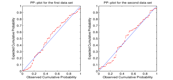
Figure 1: The PP-plots for $X$ and $Y$.

Table 7: Censored schemes and the corresponding data.

Scheme1: $R=S=[4,4,4,4,4,4,4,4,4,4]$
$i,j$	1	2	3	4	5	6	7	8	9	10
$x_{i}$	1.966	2.055	2.224	2.274	2.382	2.490	2.566	2.642	2.770	2.821
$y_{j}$	2.454	2.532	2.624	2.856	2.977	3.145	3.264	3.377	3.537	3.871
Scheme2: $R=S=[2,2,2,2,2,2,2,2,2,22]$
$i,j$	1	2	3	4	5	6	7	8	9	10
$x_{i}$	1.966	2.021	2.063	2.179	2.253	2.274	2.359	2.426	2.478	2.514
$y_{j}$	2.454	2.522	2.575	2.618	2.675	2.856	2.937	2.996	3.139	3.223

7 Conclusions

In this paper, the estimation of the stress-strength parameter for two-parameter Rayleigh distribution under progressive Type-II censoring scheme is studied. For the case that location parameters are known, the exact confidence interval of $R$ is obtained. Assuming that the location parameters are equal but unknown, different methods for the estimating of $R=P(Y<X)$ are utilized. As the MLE of $R$ can not be obtained analytically, an iterative procedure is applied to compute it. Moreover, the asymptotic confidence interval is derived by using the observed Fisher information matrix. It is observed that even for small sample sizes the asymptotic confidence intervals work quite well. Also, two bootstrap confidence intervals were proposed that their performance is quite satisfactory. Using the Gibbs sampling, the Bayes estimate of $R$ and corresponding credible interval are obtained too. The simulation results show that the MLE compares very well with the Bayes estimator in terms of biases and MSEs. Assuming that the location parameter is known, MLE, UMVUE and Bayes estimators are evaluated. The MLE provides the smallest biases and MSEs and the UMVUEs are the second best estimators. Finally, Bayesian intervals based on Lindley approximation provide the smallest average credible lengths in compare to other methods.

References

• [1] Ahmad, K.E., Fakhry, M.E. and Jaheen, Z.F. (1997). Empirical Bayes estimation of $P(Y<X)$ and characterization of Burr-Type X model. Journal of Statistical Planning and Inference. 64, 297 - 308.
• [2] Babayi, S., Khorram, E. and Tondro, F. (2014). Inference of $R=P[X<Y]$ for generalized logistic distribution. Statistics. 48, 862 - 871.
• [3] Badar, M.G. and Priest, A.M. (1982). Statistical aspects of fiber and bundle strength in hybrid composites. In: Hayashi, T., Kawata, K., Umekawa, S. (Eds.). Progress in Science and Engineering Composites. ICCM-IV, Tokyo. 1129 - 1136.
• [4] Balakrishnan, N. and Aggarwala, R. (2000). Progressive censoring: theory, methods and applications. Birkhauser, Boston.
• [5] Birnbaum, Z.W. (1956). On a use of Mann-Whitney statistics. Proceedings of the third Berkley Symposium in Mathematics, Statistics and Probability. 1, 13 - 17.
• [6] Cao, J.H. and Cheng, K. (2006). An introduction to the reliability mathematics. Beijing: Higher Education Press.
• [7] Chen, M.H. and Shao, Q.M. (1999). Monte Carlo estimation of Bayesian Credible and HPD intervals. Journal of Computational and Graphical Statistics. 8, 69 - 92.
• [8] Devroye, L. (1984). A simple algorithm for generating random variates with a log-concave density. Computing. 33, 247 - 257.
• [9] Dey, S., Dey, T. and Kundu, D. (2014). Two-parameter Rayleigh distribution: different methods of estimation. American Journal o f Mathematical and Management Sciences. 33, 55 - 74.
• [10] Efron, B. (1982). The jackknife, the bootstrap and other re-sampling plans. Philadelphia, PA: SIAM, CBMSNSF Regional Conference Series in Applied Mathematics. 34.
• [11] Geman, S. and Geman, A. (1984). Stochastic relaxation, Gibbs distributions and the Bayesian restoration of images. IEEE Transactions on Pattern Analysis and Machine Intelligence. 6, 721 - 740.
• [12] Hall, P. (1988). Theoretical comparison of bootstrap confidence intervals. Annals of Statistics. 16, 927 - 953.
• [13] Johnson, N.L., Kotz, S. and Balakrishnan, N. (1994) Continuous Univariate Distributions. 2nd ed., Wiley, NewYork.
• [14] Khan, H.M.R., Provost, S.B. and Singh, A. (2010). Predictive inference from a twoparameter Rayleigh life model given a doubly censored sample. Communications in Statistics - Theory and Methods. 39, 1237 - 1246.
• [15] Kotz, S., Lumelskii, Pensky, M. (2003). The stress-strength model and its generalization: theory and applications. World Scientific, Singapore.
• [16] Krishnamoorthy, K., Mukherjee, S., and Guo, H. (2007). Inference on reliability in two-parameter exponential stress-strength model. Metrika. 65, 261 - 273.
• [17] Kundu, D. and Gupta, R.D. (2005). Estimation of $R=P(Y<X)$ for the generalized exponential distribution. Metrika. 61, 291 - 308.
• [18] Kundu, D. and Gupta, R.D. (2006). Estimation of $R=P(Y<X)$ for Weibull distribution. IEEE Transactions on Reliability. 55, 270 - 280.
• [19] Kundu, D. and Raqab. M.Z. (2009). Estimation of $R=P(Y<X)$ for three parameter Weibull distribution. Statistics and Probability Letters. 79, 1839 - 1846.
• [20] Lindley, D.V. (1980). Approximate Bayesian methods. Trabajos de Estadistica. 3, 281 - 288.
• [21] Lio, Y.L. and Tsai, T.R. (2012). Estimation of $\delta=P(X<Y)$ for Burr XII distribution based on the progressively first failure-censored samples. Journal of Applied Statistics. 39, 309 - 322.
• [22] Panahi, H., and Asadi, A. (2011). Estimation of $R=P[Y<X]$ for two-parameter Burr Type XII Distribution. World Academy of Science, Engineering and Technology. 73, 509 - 514.
• [23] Raqab, M.Z. and Kundu, D. (2005). Comparison of different estimators of $P(Y<X)$ for a scaled Burr Type X distribution. Communications in Statistics - Simulation and Computation. 34, 465 - 483.
• [24] Raqab, M.Z., Madi, M.T. and Kundu, D. (2008). Estimation of $R=P(Y<X)$ for the 3-parameter generalized exponential distribution. Communications in Statistics - Theory and Methods. 37, 2854 - 2864.