Compound Poisson law for hitting times to periodic orbits in two-dimensional hyperbolic systems.

Abstract

We show that a compound Poisson distribution holds for scaled exceedances of observables $\phi$ uniquely maximized at a periodic point $\zeta$ in a variety of two-dimensional hyperbolic dynamical systems with singularities $(M,T,\mu)$, including the billiard maps of Sinai dispersing billiards in both the finite and infinite horizon case. The observable we consider is of form $\phi(z)=-\ln d(z,\zeta)$ where $d$ is a metric defined in terms of the stable and unstable foliation. The compound Poisson process we obtain is a Pólya-Aeppli distibution of index $\theta$. We calculate $\theta$ in terms of the derivative of the map $T$. Furthermore if we define $M_{n}=\max\{\phi,\ldots,\phi\circ T^{n}\}$ and $u_{n}(\tau)$ by $\lim_{n\to\infty}n\mu(\phi>u_{n}(\tau))=\tau$ the maximal process satisfies an extreme value law of form $\mu(M_{n}\leq u_{n})=e^{-\theta\tau}$. These results generalize to a broader class of functions maximized at $\zeta$, though the formulas regarding the parameters in the distribution need to be modified.

AMS classification numbers: 37D50, 37A25

1 Motivation and relevant works

The study of the statistical properties of 2-dimensional hyperbolic systems with singularities was motivated in large part by a desire to understand mathematical billiards with chaotic behavior. This model was introduced by Sinai in [48] and has been studied by many authors [2, 3, 51, 52, 17].

The statistical properties of chaotic dynamical systems are often described by probabilistic limit theorems. Let $(M,T,\mu)$ be a dynamical system, i.e., a transformation $T\colon M\to M$ preserving a probability measure $\mu$ on $M$. For any real-valued function $\phi$ on $M$ (often called an observable), let $X_{n}=\phi\circ T^{n}$, for any $n\geq 0$. We consider the stochastic process generated by the time-series $\{X_{n}\}$. We assume $\phi$ has a unique maximal point $\zeta$. For any fixed high threshold $u>0$, rare events can be defined as the event of the exceedance $(X_{n}>u)$, for some $n\geq 0$. Laws of rare events for chaotic dynamical systems have been investigated, with results on both hitting time statistics (HTS) and return time statistics (RTS) [24, 26, 34, 33, 37, 23, 28, 29]. Techniques from extreme value theory (EVT) have been used to understand the statistics of rare events [24, 28, 29, 37, 39, 40, 42, 27]. Extreme value theory concerns the distributional and almost sure limits of the derived time series of maxima $M_{n}:=\max\{X_{1},\cdots,X_{n}\}$. Since we are assuming $\phi$ has a unique maximum at $\zeta$ there is a close relation between extreme values of $\phi\circ T^{n}$ and visits to shrinking neighborhoods of $\zeta$.

Let $u_{n}$ be a sequence of constants defined by the requirement that $\lim_{n\to\infty}n\mu(\psi>u_{n})=\tau$. The research cited above has shown that for a variety of chaotic dynamical systems, with this scaling,

$$\lim_{n\to\infty}\mu(M_{n}\leq u_{n})=e^{-\theta\tau},$$

where $\theta\in[0,1]$. The parameter $\theta$ is called the extremal index and roughly measures the clustering of exceedances of the maxima. In fact $\frac{1}{\theta}$ is the average cluster size of exceedances given that one exceedance occurs.

For certain one-dimensional uniformly expanding maps and Anosov toral automorphisms a strict dichotomy has been observed. The dichotomy is that $\theta=1$ if $\zeta$ is not periodic and $\theta<1$ otherwise [42, 27, 29]. In this paper, we investigate the extremal index when $\zeta$ is a periodic point in the setting of two-dimensional hyperbolic systems with singularities. Poisson return time statistics for generic points in a variety of billiard systems (both polynomially and exponentially mixing) were established in [31]. Related results on Poisson return time statistics were obtained for Young Towers with polynomial tails in [47]. However the results of both works [31, 47] were limited to a full measure set of generic points, which explicitly excluded periodic orbits. This paper extends the results of [31] to the case of periodic points in a large class of billiard systems, using somewhat different techniques. For periodic points we show a compound Poisson distribution for exceedances holds and that the extremal index is determined by the Jacobian of the map $T$ along the periodic orbit (a precise formula is given in the statement of our main theorem). In [36] a similar result was shown for smooth toral automorphisms, and in fact in that setting a strict dichotomy was shown ($\theta=1$ if $\zeta$ is not periodic and $\theta<1$ otherwise). We don’t expect a dichotomy to hold in the class of hyperbolic systems with singularities, for example chaotic billiards. We expect the presence of singularities to enable a variety of extremal distributions, for example at observations maximized on singular sets. The analysis of the statistical properties of hyperbolic systems with singularities is more difficult than for smooth uniformly hyperbolic systems and the arguments of [36] do not generalize in a straightforward way. The main difficulty is caused by the singularities and the resulting fragmentation of phase space during the dynamics, which slows down the global expansion of unstable manifolds. We are able to use a growth lemma [17] to overcome these difficulties under certain other assumptions on the dynamics. Our results apply in particular to the billiard mapping of Sinai dispersing billiards with finite and infinite horizon.

1.1 Main assumptions

Let $M$ be a 2-dimensional compact Riemannian manifold, possibly with boundary. Let $\Omega\subset M$ be an open subset and let $T\colon\Omega\to M$ be a $C^{1+\gamma}$ diffeomorphism of $\Omega$ onto $T(\Omega)$ (here $\gamma\in(0,1]$). We assume that $S_{1}=M\setminus\Omega$ is a finite or countable union of smooth compact curves . Similarly, $S_{-1}=M\setminus T(\Omega)$ is a finite or countable union of smooth compact curves. If $M$ has boundary $\partial M$, it must be a subset of both $S_{1}$ and $S_{-1}$. We call $S_{1}$ and $S_{-1}$ singularity sets for the maps $T$ and $T^{-1}$, respectively. We denote by $\Omega_{i}$, $i\geq 1$, the connected components of $\Omega$; then $T(\Omega_{i})$ are the connected components of $T(\Omega)$. We assume that $T|_{\Omega}$ is time-reversible, and the restriction of the map $T$ to any component $\Omega_{i}$ can be extended by continuity to its boundary $\partial\Omega_{i}$, though the extensions to $\partial\Omega_{i}\cap\partial\Omega_{j}$ for $i\neq j$ need not agree. Similarly, for each $i$ the restriction of $T^{-1}$ to any connected component $T(\Omega_{i})$ can be extended by continuity to its boundary $\partial T(\Omega_{i})$.

Next we assume that the map $T$ is hyperbolic, as defined by Katok and Strelcyn [44]. This means that $T$ preserves a probability measure $\mu$ such that $\mu$-a.e. point $x\in M$ has two non-zero Lyapunov exponents: one positive and one negative. Also, the first and second derivatives of the maps $T$ and $T^{-1}$ do not grow too rapidly near their singularity sets $S_{1}$ and $S_{-1}$, respectively, and the $\epsilon$-neighborhood of the singularity set has measure $\mathcal{O}(\epsilon)$; this is to ensure the existence and absolute continuity of stable and unstable manifolds at $\mu$-a.e. point. Let $\mathcal{W}^{u}=\cap_{n\geq 0}T^{n}(\mathcal{M}\setminus S_{1})$. $\mathcal{W}^{u}$ is (mod 0) the union of all unstable manifolds, and we assume that the partition $\mathcal{W}^{u}$ of $M$ into unstable manifolds is measurable, so that $\mu$ induces conditional distributions on $\mu$-almost all unstable manifolds (see the definition and basic properties of conditional measures in [17, Appendix A]). Most importantly, we assume that the conditional distributions of $\mu$ on unstable manifolds $W\subset\mathcal{W}^{u}$ are absolutely continuous with respect to the Lebesgue measure on $W$. This means that $\mu$ is the so called Sinai-Ruelle-Bowen (SRB) measure.

We also assume that our SRB measure $\mu$ is ergodic and mixing. In physics terms, $\mu$ is an equilibrium state for the potential $-\ln DT_{|\mathcal{W}^{u}}$.

For $n\geq 1$, let

$$S_{n}=\cup_{i=0}^{n-1}T^{-i}S_{1}\,\,\,\,\text{ and }\,\,\,\,\,S_{-n}=\cup_{i=0}^{n-1}T^{i}S_{-1},$$

for each $n\geq 1$. Then the map $T^{n}\colon M\setminus S_{n}\to M\setminus S_{-n}$ is a $C^{1+\gamma_{0}}$ diffeomorphism.

We next make more specific assumptions on the system $(M,T,\mu)$ to give sufficient conditions for exponential decay rates of correlations, as well as for the coupling lemma. These assumptions have been made in other works in the literature [12, 15, 17, 22].

• Hyperbolic cones for $T$ of $T$. There exist two families of cones $C^{u}_{x}$ (unstable) and $C^{s}_{x}$ (stable) in the tangent spaces ${\cal T}_{x}M$, for all $x\in M\setminus S_{1}$, and there exists a constant $\Lambda>1$, with the following properties:

  • $D_{x}T(C^{u}_{x})\subset C^{u}_{Tx}$ and $D_{x}T(C^{s}_{x})\supset C^{s}_{Tx}$, wherever $D_{x}T$ exists.

  • $\|D_{x}T(v)\|\geq\Lambda\|v\|,\forall v\in C_{x}^{u},\quad\text{and}\quad\|D_{x}T^{-1}(v)\|\geq\Lambda\|v\|,\forall v\in C_{x}^{s}$.

  • These families of cones are continuous on $M$ and the angle between $C^{u}_{x}$ and $C^{s}_{x}$ is uniformly bounded away from zero.

  We say that a smooth curve $W\subset M$ is an unstable (stable) curve if at every point $x\in W$ the tangent line $\mathcal{T}_{x}W$ belongs in the unstable (stable) cone $C^{u}_{x}$ ($C^{s}_{x}$). Furthermore, a curve $W\subset M$ is an unstable (stable) manifold if $T^{-n}(W)$ is an unstable (stable) curve for all $n\geq 0$ (resp. $\leq 0$).

• Singularities. The boundary $\partial M$ is transversal to both stable and unstable cones. Every other smooth curve $W\subset S_{1}\setminus\partial M$ (resp. $W\subset S_{-1}\setminus\partial M$ ) is a stable (resp. unstable) curve. Every curve in $S_{1}$ terminates either inside another curve of $S_{1}$ or on the boundary $\partial M$. A similar assumption is made for $S_{-1}$. Moreover, there exists $C>0$ such that for any $x\in M\setminus S_{1}$

  $$\|D_{x}T\|\leq C\,\text{\rm dist}(x,S_{1})^{-1},$$ (1)

  and for any $\epsilon>0$,

  $$\mu\bigl{(}x\in M\colon\text{\rm dist}(x,S_{1})<\varepsilon\bigr{)}<C\epsilon.$$ (2)

  Note that (2) implies that for $\mu$-a.e. $x\in M$, there exists a stable and unstable manifold $W^{u/s}(x)$, such that $T^{n}W^{s}(x)$ and $T^{-n}W^{u}(x)$ does not intersect $S_{1}$, for any $n\geq 0$.

  Definition 1.

  For every $x,y\in M$, define $\mathbf{s}_{+}(x,y)$, the forward separation time of $x,y$, to be the smallest integer $n\geq 0$ such that $x$ and $y$ belong to distinct elements of $M\setminus S_{n}$. Fix $\beta\in(0,1)$, then $d(x,y)=\beta^{\mathbf{s}_{+}(x,y)}$ defines a metric on $M$. Similarly we define the backward separation time $\mathbf{s}_{-}(x,y)$.

• Regularity of stable/unstable curves. We assume that the following families of stable/unstable curves, denoted by $\mathcal{W}^{s,u}_{T}$ are invariant under $T^{-1}$ (resp., $T$) and include all stable/unstable manifolds:

  1. Bounded curvature. There exist $B>0$ and $c_{M}>0$, such that the curvature of any $W\in\mathcal{W}^{s,u}_{T}$ is uniformly bounded from above by $B$, and the length of the curve $|W|<c_{M}$.

  2. Distortion bounds. There exist $\gamma_{0}\in(0,1)$ and $C_{\mathbf{r}}>1$ such that for any unstable curve $W\in\mathcal{W}^{u}_{T}$ and any $x,y\in W$,

     $$\left|\ln\mathcal{J}_{W}(T^{-1}x)-\ln\mathcal{J}_{W}(T^{-1}y)\right|\leq C_{\mathbf{r}}\,\text{\rm dist}(x,y)^{\gamma_{0}}$$ (3)

     where $\mathcal{J}_{W}(T^{-1}x)=dm_{T^{-1}W}(T^{-1}x)/dm_{W}(x)$ denotes the Jacobian of $T^{-1}$ at $x\in W$ with respect to the Lebesgue measure $m_{W}$ on the unstable curve $W$.

  3. Absolute continuity. Let $W_{1},W_{2}\in\mathcal{W}^{u}_{T}$ be two unstable curves close to each other. Denote

     $$W_{i}^{\prime}=\{x\in W_{i}\colon W^{s}(x)\cap W_{3-i}\neq\emptyset\},\hskip 14.22636pti=1,2.$$

     The map $\mathbf{h}\colon W_{1}^{\prime}\rightarrow W_{2}^{\prime}$ defined by sliding along stable manifolds is called the holonomy map. We assume $\mathbf{h}_{*}\mu_{W_{1}^{\prime}}\prec\mu_{W_{2}^{\prime}}$, and furthermore, there exist uniform constants $C_{\mathbf{r}}>0$ and $\vartheta_{0}\in(0,1)$, such that the Jacobian of $\mathbf{h}$ satisfies

     $$|\ln\mathcal{J}\mathbf{h}(y)-\ln\mathcal{J}\mathbf{h}(x)|\leq C_{\mathbf{r}}\vartheta_{0}^{\mathbf{s}_{+}(x,y)},\hskip 28.45274pt\forall x,y\in W_{1}^{\prime}$$ (4)

     Similarly, for any $n\geq 1$ we can define the holonomy map

     $$\mathbf{h}_{n}=T^{n}\circ\mathbf{h}\circ T^{-n}:T^{n}W_{1}\to T^{n}W_{2},$$

     and then (4) and the uniform hyperbolicity (h1) imply

     $$\ln\mathcal{J}\mathbf{h}_{n}(T^{n}\mathbf{x})\leq C_{\mathbf{r}}\vartheta_{0}^{n}$$ (5)

• One-step expansion. We have

  $$\liminf_{\delta\to 0}\ \sup_{W\colon|W|<\delta}\sum_{n}\frac{|T^{-1}V_{n}|}{|V_{n}|}<1,$$ (6)

  where the supremum is taken over regular unstable curves $W\subset M$, $|W|$ denotes the length of $W$, and $V_{n}$, $n\geq 1$, denote the smooth components of $T(W)$.

Remark 1.

These assumptions $\textbf{h1}-$h4 are satisfied by the billiard map associated to Sinai dispersing billiards with finite and infinite horizon. Further systems which satisfy these assumptions are given in the last section on applications.

Remark 2.

These assumptions $\textbf{h1}-$h4 along with the Growth Lemma imply the existence of a Young Tower with exponential tails [22, Lemma 17].

1.2 Statement of the main results

We fix a hyperbolic periodic point $\zeta\in M$ with prime period $q>1$, and let $\phi:M\to\mathbb{R}\cup\{+\infty\}$ be given by

$$\phi(z)=-\ln(d(z,\zeta)),$$

where $d$ is a metric on $M$ that will be specified later. We assume that iterates of $\zeta$ do not lie on the singular sets $S_{1}\cup S_{-1}$. Our metric $d$ will be adapted to the chart given by the stable and unstable manifolds of $\zeta$, denoted as $W^{s}(\zeta)$ and $W^{u}(\zeta)$. If the stable manifold of $x$, denoted as $W^{s}(x)$ intersects $W^{u}(\zeta)$, say at a point $z$, then we define $x^{s}:=\text{\rm dist}_{W^{u}(\zeta)}(z,\zeta)$, i.e. the distance of $z$ and $\zeta$ measured along the unstable manifold $W^{u}(\zeta)$. Note that if $W^{u}(x)$ is very short and does not reach $W^{s}(\zeta)$, then we may extend $W^{u}(x)$ as an unstable curve, thus $x^{u}$ can be similarly defined. If the unstable manifold (or extension to an unstable curve) of $x$, denoted as $W^{u}(x)$ intersects $W^{s}(\zeta)$ at $z$, we define $x^{u}:=\text{\rm dist}_{W^{s}(\zeta)}(z,\zeta)$. The foliation of stable and unstable curves of a sufficiently small neighborhood of $\zeta$ will be Hölder continuous. Moreover, if both $x$, $y$ lie in the same local chart determined by stable and unstable manifolds (or stable and unstable curves) so that $x=(x^{u},x^{s})$, $y=(y^{u},y^{s})$, we define

$$d(x,y)=\max\{|x^{u}-y^{u}|,|y^{s}-y^{s}|\}.$$ (7)

As in [36] we expect the form of the distribution for cluster size in the compound Poisson distribution we obtain to depend upon the metric used. With the dynamically adapted metric we use we obtain a geometric distribution with parameter equal to the extremal index $\theta$, $\theta=1-\frac{1}{|DT^{q}_{u}(\zeta)|}$, where $DT^{q}_{u}(\zeta)$ is the derivative of $T^{q}$ in the unstable direction at $\zeta$. With the usual Euclidean metric $\rho$ we would expect a different distribution along the lines of the (complicated) calculations in [36, Section 6].

The functional form of $\phi$ will determine the scaling constants in the extreme value distribution but results for one functional type are easily transformed into any other, see for example [39, 28]. Let $X_{n}:=\phi\circ T^{n}$. Since $\mu$ is invariant the process $\{X_{n},n\geq 0\}$ is stationary. Note that $\{X_{n}>u\}=T^{-n}(B_{e^{-u}}(\zeta))$, where $B_{e^{-u}}(\zeta)$ denotes the $d$-ball centered at $\zeta$ of radius $e^{-u}$. In order to obtain a nondegenerate limit for the distribution of $M_{n}=\max\{X_{0},\cdots,X_{n}\}$, we choose a normalizing sequence $\{u_{n}\}=\{u_{n}(\tau)\}$ such that

$$u_{n}=u_{n}(\tau):=\inf\{u>0\,:\,\mu(X_{0}\leq u)\geq 1-\frac{\tau}{n}\}$$

for any $\tau>0$. We also define

$$U_{n}(\tau)=(X_{0}>u_{n}(\tau))$$

Then we can check that

$$\lim_{n\to\infty}n\mu(X_{0}>u_{n})=\lim_{n\to\infty}n\mu(U_{n})=\tau$$ (8)

The extremal index, written as $\theta$, takes values in $[0,1]$, and can be interpreted as an indicator of extremal dependence, with $\theta=1$ indicating asymptotic independence of extreme events. On the other hand $\theta=0$ represents the case where we can expect strong clusterings of extreme events. In this case it is natural to expect excursions away from moderate values to extreme regions to persist for random times which have heavy-tailed distributions.

Note that the choice of $u_{n}$ is made so that the mean number of exceedances by $X_{0},\cdots,X_{n}$ is approximately constant. For the case when $\{X_{n}\}$ are iid, it was shown in [45] that (8) is equivalent to the fact that $\mu(M_{n}\leq u_{n})\to e^{-\tau}$ as $n\to\infty$. We are interested in knowing if there is a non-degenerate distribution $H$ such that the scaled process $\mu(M_{n}\leq u_{n})$ converges in distribution to $H$ as $n$ goes to infinity. Then we say that $H$ is an Extreme Value Distribution for $M_{n}$. Note that by the Birkhoff Ergodic Theorem, we know that $M_{n}\to\max\{\phi(\zeta),\infty\}$ almost surely and hence we must scale $u_{n}\to\max\{\phi(\zeta),\infty\}$ as $n\to\infty$. We refer the event $\{X_{j}>u\}$ as an exceedance at time $j$ of level $u$.

The assumption that $\zeta$ is a hyperbolic $q$-periodic point, the assumptions (h1)-(h4) and the definition of the $d$-metric implies that there exists $\theta\in(0,1)$, such that

$$\lim_{n\to\infty}\mu(X_{q}>u_{n}|X_{0}>u_{n})=1-\theta$$ (9)

$\theta=1-\frac{1}{|DT^{q}_{u}(\zeta)|}$, where $DT^{q}_{u}(\zeta)$ is the derivative of $T^{q}$ in the unstable direction at $\zeta$. The calculation is the same as in [36, Section 6].

Our first theorem is

Theorem 1.

Let $\zeta$ be a periodic orbit of period $q$, $q\not\in S_{1}\cup S_{-1}$, and define

$$\phi(z)=-\ln(d(z,\zeta)),$$

where $d$ is the metric adapted to the chart given by the stable and unstable foliation. Define $M_{n}:=\max\{\phi,\ldots,\phi\circ T^{n-1}\}$. Then

$$\lim_{n\to\infty}\mu(M_{n}\leq u_{n})=e^{-\theta\tau},$$

where $\theta=1-\frac{1}{|DT^{q}_{u}(\zeta)|}$.

Now we consider the related rare event point processes (REPP). Let $N_{n}$ be the number of exceedances of a level $u_{n}$ by the process $X_{0},\cdots,X_{n}$. If $\{X_{n}\}$ is an i.i.d. sequence, it was proved in [45] that if $u_{n}$ satisfies $n\mu(X_{0}>u_{n})\to\tau$ as $n\to\infty$, then $N_{n}$ follows a Poisson distribution with intensity $\tau$:

$$\mu(N_{n}\leq k)\to e^{-\tau}\sum_{i=0}^{k}\frac{\tau^{i}}{i!},$$

for any $k\geq 0$. On the other hand, for a stationary process $\{X_{n}\}$ with clustering of recurrence we expect that $N_{n}$ converges to a compound Poisson distribution. This behavior has been observed in a variety of one-dimensional expanding maps [29, 27, 42] as well as in two-dimensional hyperbolic linear toral automorphisms [34, 26, 36]. In fact in these papers a strict dichotomy has been observed in the extreme value statistics of functions maximized at periodic as opposed to non-periodic points. In this paper we show that a compound Poisson process governs the return times to periodic points for a large class of two-dimensional invertible hyperbolic systems. As we mentioned the precise form of the compound Poisson process depends upon the metric used. For simplicity we consider a dynamically adapted metric $d$, which yields a geometric distribution for the cluster size of exceedances with parameter $\theta$. Other distributions for the cluster size would be expected with different metrics, as in [36, Section 6].

To make precise our statements we need the following definitions. Denote by $\mathcal{R}$ the ring generated by intervals of the type $[a,b)$, for $a,b\in\mathbf{R}_{0}^{+}$. Thus for every $J\in\mathcal{R}$ there are $k$ intervals $I_{1},\ldots,I_{k}\in\mathcal{S}$, say $I_{j}=[a_{j},b_{j})$ with $a_{j},b_{j}\in\mathbf{R}_{0}^{+}$, such that $J=\cup_{i=1}^{k}I_{j}$. For $I=[a,b)$ and $\alpha\in\mathbf{R}$, we set $\alpha I:=[\alpha a,\alpha b)$ and $I+\alpha:=[a+\alpha,b+\alpha)$. Similarly, for $J\in\mathcal{R}$, we define $\alpha J:=\alpha I_{1}\cup\cdots\cup\alpha I_{k}$ and $J+\alpha:=(I_{1}+\alpha)\cup\cdots\cup(I_{k}+\alpha)$.

Definition 2.

Given $J\in\mathcal{R}$ and a sequence $(u_{n})_{n\in\mathbf{N}}$, the rare event point process (REPP) is defined by counting the number of exceedances (or events $(X_{i}>u_{n})$) during the (re-scaled) time period $u_{n}^{-1}J\in\mathcal{R}$. More precisely, for every $J\in\mathcal{R}$, set

$$N_{n}(J):=\sum_{i\in u_{n}^{-1}J\cap\textbf{}N_{0}}\mathbbm{1}_{X_{i}>u_{n}}.$$ (10)

For the sake of completeness, we also define what we mean by a Poisson and a compound Poisson process.

Definition 3.

Let $Y_{1},Y_{2},\ldots$ be an iid sequence of random variables with common exponential distribution of mean $1/\vartheta$. Let $Z_{1},Z_{2},\ldots$ be another iid sequence of random variables, independent of $(Y_{i})$, and with distribution function $G$. Given these sequences, for $J\in\mathbf{R}$ define

$$N(J)=\int\mathbbm{1}_{J}\;d\left(\sum_{i=1}^{\infty}Z_{i}\delta_{Y_{1}+\ldots+Y_{i}}\right),$$

where $\delta_{t}$ denotes the Dirac measure at $t>0$. We say that $N$ is a compound Poisson process of intensity $\vartheta$ and multiplicity d.f. $G$.

Remark 3.

In our context we think of the random variable $Z_{i}$ as determining the number of exceedances given that one has occurred in a certain time interval.

Remark 4.

In our setting $Z_{i}$ will always be integer valued, as it gives the size of a cluster. This means that $\Lambda$ is completely defined by the values $G(k)=P(Z_{1}=k)$, for every $k\in\textbf{}N_{0}$. Note that, if $G(1)=1$ and $\vartheta=1$, then $N$ is the standard Poisson process and, for every $t>0$, the random variable $N([0,t))$ has a Poisson distribution of mean $t$.

Remark 5.

In this paper $G$ turns out to be a geometric distribution of parameter $\theta\in(0,1]$, i.e. $G(k)=\theta(1-\theta)^{k-1}$, for every $k\in\textbf{}N_{0}$. This means that, as in [32, 36], the random variable $N([0,t))$ follows a Pólya-Aeppli distribution

$$P(N([0,t)))=k=e^{-\theta t}\sum_{j=1}^{k}\theta^{j}(1-\theta)^{k-j}\frac{(\theta t)^{j}}{j!}\binom{k-1}{j-1},$$

for all $k\in\textbf{}N$, and that $P(N([0,t))=0)=e^{-\theta t}$. So there is just one parameter $\theta$ governing the compound Poisson distribution.

Theorem 2.

Let $\zeta$ be a periodic orbit of period $q$, $q\not\in S_{1}\cup S_{-1}$, and

$$\phi(z)=-\ln(d(z,\zeta))$$

where $d$ is the metric adapted to the chart given by the stable and unstable foliation. Define $X_{n}=\phi\circ T^{n}$ and $M_{n}:=\max\{X_{1},\ldots,X_{n}\}$. Let $(u_{n})_{n\in\textbf{}N}$ be a sequence satisfying $\lim_{n\to\infty}n\mu(X_{0}>u_{n})=\tau$ for some $\tau\geq 0$ and $(v_{n})_{n\in\textbf{}N}$ be given by $v_{n}=1/\mu(X_{0}>u_{n})$. Consider the REPP $N_{n}$ as in Definition 2. Then the REPP $N_{n}$ converges in distribution to a compound Poisson process with intensity $\theta=1-\frac{1}{|DT^{q}_{u}(\zeta)|}$ and geometric multiplicity d.f. $G^{*}$ given by $G^{*}(k)=\theta(1-\theta)^{k-1}$, for all $k\in\textbf{}N$.

2 Extreme value theory scheme of proof.

Our proofs are based on ideas from extreme value theory. Let $X_{n}=\phi\circ T^{n}$ and define $A_{n}^{q}:=\{X_{0}>u_{n},X_{q}\leq u_{n}\}$. For $s,l\in\mathbb{N}$ and a set $B\subset M$, let

$$\mathscr{W}_{s,l}(B)=\bigcap_{i=s}^{s+l-1}T^{-i}(B).$$

Next we introduce two conditions following [36].

Condition $\operatorname{\textrm{Д}}_{q}(u_{n})$: We say that $\operatorname{\textrm{Д}}_{q}(u_{n})$ holds for the sequence $X_{0},X_{1},\ldots$ if, for every $\ell,t,n\in\mathbb{N}$

$$\left|\mu\left(A_{n}^{q}\cap\mathscr{W}_{t,\ell}\left(A_{n}^{q}\right)\right)-\mu\left(A_{n}^{q}\right)\mu\left(\mathscr{W}_{0,\ell}\left(A_{n}^{q}\right)\right)\right|\leq\gamma(q,n,t),$$

where $\gamma(q,n,t)$ is decreasing in $t$ and there exists a sequence $(t_{n})_{n\in\mathbb{N}}$ such that $t_{n}=o(n)$ and $n\gamma(q,n,t_{n})\to 0$ when $n\rightarrow\infty$.

We consider the sequence $(t_{n})_{n\in\textbf{}N}$ given by condition $\operatorname{\textrm{Д}}_{q}(u_{n})$ and let $(k_{n})_{n\in\textbf{}N}$ be another sequence of integers such that as $n\to\infty$,

$$k_{n}\to\infty\quad\mbox{and}\quad k_{n}t_{n}=o(n).$$

Condition $\operatorname{\textrm{Д}}^{\prime}_{q}(u_{n})$: We say that $\operatorname{\textrm{Д}}^{\prime}_{q}(u_{n})$ holds for the sequence $X_{0},X_{1},\ldots$ if there exists a sequence $(k_{n})_{n\in\textbf{}N}$ as above and such that

$$\lim_{n\rightarrow\infty}\,n\sum_{j=1}^{\lfloor n/k_{n}\rfloor}\mu\left(A_{n}^{q}\cap T^{-j}\left(A_{n}^{q}\right)\right)=0.$$

We note that, when $q=0$, which corresponds to a non-periodic point, condition $\operatorname{\textrm{Д}}^{\prime}_{q}(u_{n})$ corresponds to condition $D^{\prime}(u_{n})$ from [45].

Now let

$$\theta=\lim_{n\to\infty}\theta_{n}=1-\lim_{n\to\infty}\frac{\mu(A^{q}_{n})}{\mu(U_{n})}.$$

From [29, Corollary 2.4], it follows that to proof Theorem 1 it suffices to prove conditions $\operatorname{\textrm{Д}}_{q}(u_{n})$ and $\operatorname{\textrm{Д}}^{\prime}_{q}(u_{n})$ since if both conditions hold then from [29, Corollary 2.4] the limit exists and

$$\lim_{n\to\infty}\mu(M_{n}\leq u_{n})=e^{-\theta\tau}.$$

To establish Theorem 2 it suffices to establish Condition $\operatorname{\textrm{Д}}^{\prime}_{q}(u_{n})$ and a property related to Condition $\operatorname{\textrm{Д}}_{q}(u_{n})$, which we call Condition $\operatorname{\textrm{Д}}^{*}_{q}(u_{n})$ [30] (see also the discussion in [36, Section 8.1]). We state $\operatorname{\textrm{Д}}^{*}_{q}(u_{n})$ for completeness, but its proof is a decay of correlations result which requires only very minor modifications to that of the proof of Condition $\operatorname{\textrm{Д}}_{q}(u_{n})$. We will only prove Condition $\operatorname{\textrm{Д}}_{q}(u_{n})$ in this paper. The proof of Condition $\operatorname{\textrm{Д}}_{q}(u_{n})$ uses the assumption of a Young Tower to approximate the indicator function of a complicated set by a function constant on stable manifolds, which allows a decay rate to be bounded by the $L^{\infty}$ norm of the set rather than a Hölder norm. In fact the scheme of the proof of Condition $\operatorname{\textrm{Д}}_{q}(u_{n})$ is itself somewhat standard [31, 36] and the novelty of this paper is the proof of Condition $\operatorname{\textrm{Д}}^{\prime}_{q}(u_{n})$ in this setting, which uses the growth lemma of [17] applied to unstable curves.

Let $\zeta$ be a periodic point of prime period $q$. Recall $U_{n}=(X_{0}>u_{n})$ and define the sequence $U^{(k)}(u_{n}))$ of nested sets centered at $\zeta$ given by

$$U^{(0)}(u_{n})=U_{n}\quad\text{and}\quad U^{(k)}(u_{n})=T^{-q}(U^{(k-1)}(u_{n}))\cap U_{n},\quad\text{for all $k\in\mathbb{N}$.}$$ (11)

For $i,k,l,s\in\mathbb{N}\cup\{0\}$, we define the following sets:

$$Q_{q,i}^{k}(u_{n}):=T^{-i}\left(U^{(k)}(u_{n})-U^{(k+1)}(u_{n})\right).$$ (12)

Note that $Q_{q,0}^{0}(u_{n})=A_{n}^{(q)}$. Furthermore, $U_{n}=\bigcup_{k=0}^{\infty}Q_{q,0}^{k}(u_{n})$. Using our $d$-metric the set $U_{n}$ centered at $\zeta$ can be decomposed into a sequence of disjoint strips where $Q_{q,0}^{0}(u_{n})$ are the most outward strips and the inner strips $Q_{q,0}^{k+1}(u_{n})$ are sent outward by $T^{q}$ onto the strips $Q_{q,0}^{k}(u_{n})$, i.e., $T^{q}(Q_{q,0}^{k+1}(u_{n}))=Q_{q,0}^{k}(u_{n}).$

Definition 4 ($D_{q}(u_{n})^{*}$).

We say that $D_{q}(u_{n})^{*}$ holds for the sequence $X_{0},X_{1},X_{2},\ldots$ if for any integers $t,k_{1},\ldots,k_{q}$, $n$ and any $J=\cup_{j=2}^{q}I_{j}\in\mathbf{R}$ with $\inf\{x:x\in J\}\geq t$,

$$\left|P\left(Q_{q,0}^{k_{1}}(u_{n})\cap\left(\cap_{j=2}^{q}N_{n}(I_{j})=k_{j}\right)\right)-P\left(Q_{q,0}^{k_{1}}(u_{n})\right)P\left(\cap_{j=2}^{q}N_{n}(I_{j})=k_{j}\right)\right|\leq\gamma(n,t),$$

where for each $n$ we have that $\gamma(n,t)$ is nonincreasing in $t$ and $n\gamma(n,t_{n})\to 0$ as $n\rightarrow\infty$, for some sequence $t_{n}=o(n)$.

3 Background on billiards: growth lemma and decay of correlations for hyperbolic billiards.

The use of standard pairs of unstable and stable curves  [17] instead of standard pairs of unstable and stable manifolds simplifies our proof of Condition $\operatorname{\textrm{Д}}_{q}^{\prime}(u_{n})$. We now sketch some background on the use of standard pairs.

For any $\gamma\geq\gamma_{0}$, let $\mathcal{H}^{-}(\gamma)$ be the set of all bounded real-valued functions $\varphi\in L_{\infty}(\mathcal{M},\mu)$ such that for any $x$ and $y$ lying on one stable curve $W^{s}\in\mathcal{W}^{s}_{T}$, such that

$$\|\varphi\|^{-}_{\gamma}\colon=\sup_{W^{s}\in\mathcal{W}^{s}_{T}}\sup_{x,y\in W^{s}}\frac{|\varphi(x)-\varphi(y)|}{\text{\rm dist}(x,y)^{\gamma}}<\infty.$$

and

$$|\varphi(x)-\varphi(y)|\leq\|\varphi\|^{-}_{\gamma}\text{\rm dist}(x,y)^{\gamma}$$ (13)

Similarly we define $\mathcal{H}^{+}(\gamma)$ as the set of all real-valued functions $\psi\in L_{\infty}(\mathcal{M},\mu)$ such that for any $x$ and $y$ lying on one unstable curve $W^{u}\in\mathcal{W}^{u}_{T}$ such that

$$\|\psi\|^{+}_{\gamma}\colon=\sup_{W^{u}\in\mathcal{W}^{u}_{T}}\sup_{x,y\in W^{u}}\frac{|\psi(x)-\psi(y)|}{\text{\rm dist}(x,y)^{\gamma}}<\infty,$$

and

$$|\psi(x)-\psi(y)|\leq\|\psi\|^{+}_{\gamma}\text{\rm dist}(x,y)^{\gamma}.$$ (14)

When we study autocorrelations of certain observables, we will need to require that the latter belong to the space $\mathcal{H}(\gamma)\colon=\mathcal{H}^{+}(\gamma)\cap\mathcal{H}^{-}(\gamma)$, i.e., they are Hölder functions on every stable and unstable manifold. For correlations of two distinct functions $\varphi$, $\psi$ as above we always assume that $\varphi\in\mathcal{H}^{-}(\gamma_{1})$ and $\psi\in\mathcal{H}^{+}(\gamma_{2})$ with some $\gamma_{1},\gamma_{2}\in[\gamma_{0},1]$, unless otherwise specified. For every $\varphi\in\mathcal{H}^{\pm}(\gamma)$ we define

$$\|\varphi\|^{\pm}_{C^{\gamma}}\colon=\|\varphi\|_{\infty}+\|\varphi\|^{\pm}_{\gamma}.$$ (15)

By using coupling methods, we obtain the following bounds for the rate of decay of correlations for our class of hyperbolic systems with singularities, see [22].

Lemma 3.

For systems satisfy (h1)- (h4), there exist $C>0$, $p\in(0,1)$, such that for any observables $\varphi\in\mathcal{H}^{-}(\gamma_{1})$ and $\psi\in\mathcal{H}^{+}(\gamma_{2})$ on $\mathcal{M}$, with $\gamma_{i}\in[\gamma_{0},1]$, for $i=1,2$,

$$|\int\psi\cdot\varphi\circ T^{n}d\mu-\int\psi d\mu\int\phi d\mu|\leq C\|\psi\|^{+}_{{}_{C^{\gamma_{2}}}}\|\varphi\|^{-}_{{}_{C^{\gamma_{1}}}}\Lambda^{-pn}$$ (16)

for any $n\geq 1$.

Let $C_{\mathbf{r}}>0$ and $\gamma_{0}\in(0,1)$ be the constants given in (3). Fix a large constant $C_{\mathbf{J}}>C_{\mathbf{r}}/(1-1/\Lambda)$. Given an unstable curve $W$ and a probability measure $\nu$ on $W$, the pair $(W,\nu)$ is said to be a standard pair if $\nu$ is absolutely continuous with respect to $\mu_{W}$, such that the density function $g_{W}(x):=d\nu/d\mu_{W}(x)$ is regular in the sense that

$$|\ln g_{W}(x)-\ln g_{W}(y)|\leq C_{\mathbf{J}}\cdot d_{W}(x,y)^{\gamma_{0}}.$$ (17)

Iterates of standard pairs require the following extension of standard pairs, see [17, 22]. Let $\mathcal{G}=\{(W_{\alpha},\nu_{\alpha}),\ \alpha\in\mathcal{A},\ \lambda\}$ be a family of standard pairs equipped with a factor measure $\lambda$ on the index set $\mathcal{A}$. We call $\mathcal{G}$ a standard family if the following conditions hold:

1. $\mathcal{W}:=\{W_{\alpha}:\alpha\in\mathcal{A}\}$ is a measurable partition into unstable curves;

2. There is a finite Borel measure $\nu$ supported on $\mathcal{W}$ such that for any measurable set $B\subset M$,

   $$\nu(B)=\int_{\alpha\in\mathcal{A}}\nu_{\alpha}(B\cap W_{\alpha})\,d\lambda(\alpha).$$

For simplicity, we denote such a family by $\mathcal{G}=(\mathcal{W},\nu)$.

Given a standard family $\mathcal{G}=(\mathcal{W},\nu)=\{(W_{\alpha},\nu_{\alpha}),\ \alpha\in\mathcal{A},\ \lambda\}$ and $n\geq 1$, the forward image family $T^{n}\mathcal{G}=(\mathcal{W}_{n},\nu_{n})=\{(V_{\beta},\nu^{n}_{\beta}),\ \beta\in\mathcal{B},\ \lambda^{n}\}$ is such that each $V_{\beta}$ is a connected component of $T^{n}W_{\alpha}\backslash S_{-n}$ for some $\alpha\in\mathcal{A}$, associated with $\nu^{n}_{\beta}(\cdot)=T^{n}_{*}\nu_{\alpha}(\cdot\ |\ V_{\beta})$ (where $T^{n}_{*}\nu_{\alpha}$ is the pushforward of $\nu_{\alpha}$ to $T^{n}W_{\alpha}$ ) and $d\lambda^{n}(\beta)=\nu_{\alpha}(T^{-n}V_{\beta})d\lambda(\alpha)$. It is not hard to see that $T^{n}\mathcal{G}$ is a standard family as well (cf. [17]).

Let $\mathfrak{F}$ be the collection of all standard families. We introduce a characteristic function on $\mathfrak{F}$ to measure the average length of unstable curves in a standard family. More precisely, we define a function $\mathcal{Z}:\mathfrak{F}\to[0,\infty]$ by

$$\mathcal{Z}(\mathcal{G})=\dfrac{1}{\nu(M)}\int_{\mathcal{A}}|W_{\alpha}|^{-1}\,d\lambda(\alpha),\ \ \text{for any}\ \mathcal{G}\in\mathfrak{F}.$$ (18)

where $\mathbf{s}_{0}$ is as in assumption (h2). Let $\mathfrak{F}_{0}$ denote the class of $\mathcal{G}\in\mathfrak{F}$ such that $\mathcal{Z}(\mathcal{G})<\infty$.

It turns out that the value of $\mathcal{Z}(T^{n}\mathcal{G})$ decreases exponentially in $n$ until it becomes small enough. This fundamental fact, called the growth lemma, was first proved by Chernov for dispersing billiards in [12], and later proved in [17] under Assumptions (h1)-(h4).

Lemma 4.

There exist constants $c>0$, $C_{z}>0$, and $\vartheta\in(0,1)$ such that for any $\mathcal{G}\in\mathfrak{F}_{0}$,

$$\mathcal{Z}(T^{n}\mathcal{G})\leq c\vartheta^{n}\mathcal{Z}(\mathcal{G})+C_{z},\ \ \ \text{for any}\ n\geq 0.$$

4 Checking condition $\operatorname{\textrm{Д}}_{q}(u_{n})$

The proof of Condition $\operatorname{\textrm{Д}}_{q}(u_{n})$ uses decay of correlations and is fairly standard. The following analysis is taken from [31] but is included for completeness. The proof considers stable manifolds rather than stable curves, as well as ideas from Young’s Tower construction for billiard systems [51]. Recall that assumptions $(\textbf{h1})-$$(\textbf{h4})$ along with the Growth Lemma imply the existence of a Young Tower with exponential tails [22, Lemma 17]. Throughout this section, to simplify notation, $C$ will denote an unspecified constant, whose value may vary from line to line.

We now briefly the structure of a Young Tower with exponential return time tails for a map $T:M\to M$ of a Riemannian manifold $M$ equipped with Lebesgue measure $m$.

A Young Tower has a base set $\Delta_{0}$ with a hyperbolic product structure as in Young [51] with an $\mathscr{L}^{1}(m)$ return time function $R:\Delta_{0}\to\mathbb{N}$. There is a countable partition $\Lambda_{0,i}$ of $\Delta_{0}$ so that $R$ is constant on each partition element $\Lambda_{0,i}$. We denote $R|_{\Lambda_{0,i}}$ by $R_{i}$. The Young Tower is defined by

$$\Delta=\bigcup_{i\in\textbf{}N,0\leq l\leq R_{i}-1}\{(x,l):x\in\Lambda_{0,i}\}$$

equipped with a tower map $F:\Delta\to\Delta$ given by

$$F(x,l)=\begin{cases}(x,l+1)&\mbox{ if }x\in\Lambda_{0,i},l<R_{i}-1\\ (T^{R_{i}}x,0)&\mbox{ if }x\in\Lambda_{0,i},l=R_{i}-1\end{cases}.$$

We will refer to $\Delta_{0}:=\cup_{i}(\Lambda_{0,i},0)$ as the base of the tower $\Delta$ and denote $\Lambda_{i}:=\Lambda_{0,i}$. Similarly we call $\Delta_{l}=\{(x,l):l<R(x)\}$, the $l-$th level of the tower. A key role is played by the return map $f=T^{R}:\Delta_{0}\to\Delta_{0}$ by $f(x)=T^{R(x)}(x)$, which is uniformly expanding Gibbs-Markov.

We may form a quotiented tower (see [51] for details) by introducing an equivalence relation for points on the same stable manifold. This operation helps in our decay of correlations estimates, as it allows decay rates for the indicator function of complicated sets to be estimated in the $L^{\infty}$ norm.We now list the features of the Tower that we will use.

There exists an invariant measure $m_{0}$ for $f:\Delta_{0}\to\Delta_{0}$ which has absolutely continuous conditional measures on local unstable manifolds in $\Delta_{0}$, with density bounded uniformly from above and below.

There exists an $F$-invariant measure $\nu$ on $\Delta$ which is given by $\nu(B)=\frac{m_{0}(F^{-l}B)}{\int_{\Lambda_{0}}R\,dm_{0}}$ for a measurable $B\subset\Lambda_{l}$, and extended to the entire tower $\Delta$ in the obvious way. There is a projection $\pi:\Delta\to M$ given by $\pi(x,l)=T^{l}(x)$ which semi-conjugates $F$ and $T$, so that $\pi\circ F=T\circ\pi$. The invariant measure $\mu$, which is an SRB measure for $T:M\to M$, is given by $\mu=\pi_{*}\nu$. Denote by $W^{s}(x)$ the local stable manifold through $x$ and by $W^{u}(x)$ the local unstable manifold. Let $B(x,r)$ denote the ball of radius $r$ centered at the point $x$.

We lift a function $\phi:M\to\mathbf{R}$ to $\Delta$ by defining $\phi(x,l)=\phi(T^{l}x)$ (we keep the same symbol for $\phi$ on $\Delta$ and $\phi$ on $M$).

Under the assumption of exponential tails, that is if $m(R>n)=\mathcal{O}(\gamma_{1}^{n})$ for some $0<\gamma_{1}<1$ then Young shows [51] there exists $0<\Lambda_{1}<1$ such that for all Lipschitz $\phi$, $\psi$ we have

$$\left|\int\phi\psi\circ T^{n}d\mu-\int\phi d\mu\int\psi d\mu\right|\leq C\Lambda_{1}^{n}\|\phi\|_{Lip}\|\psi\|_{Lip}$$ (19)

for some constant $C$. Moreover, if the lift of $\psi$ is constant on local stable leaves of the Young Tower, then

$$\left|\int\phi\psi\circ T^{n}\,d\mu-\int\phi\,d\mu\int\psi\,d\mu\right|\leq C\Lambda_{2}^{n}\|\phi\|_{Lip}\|\psi\|_{\infty}.$$ (20)

Let $D$ be a set whose boundary is piecewise smooth and finite length, and define

$$H_{k}(D)=\left\{x\in D:T^{k}(W^{s}(x))\cap\partial D\not=\emptyset\right\}.$$

Proposition 5.

There exist constants $C>0$ and $0<\tau_{1}<1$ such that, for all $k$,

$$\mu(H_{k}(D))\leq C\tau_{1}^{k}.$$ (21)

Proof.

As a consequence of the uniform contraction of local stable manifolds, there exists $0<\tau_{1}<1$ and $C_{1}>0$ such that $\text{\rm dist}\,(T^{n}(x),T^{n}(y))\leq C_{1}\tau_{1}^{n}$ for all $y\in W^{s}(x).$ In particular, this implies that $|T^{k}(W^{s}(x))|\leq C_{1}\tau_{1}^{k}$. Therefore, for every $x\in H_{k}(D)$, the stable manifold $T^{k}(W^{s}(x))$ lies in an “annulus” of width $2\tau_{1}^{k}$ around $\partial D$. By the invariance of $\mu$ the result follows.

∎

Lemma 6.

Suppose $\Phi:M\to\mathbf{R}$ is a Lipschitz map and $\Psi$ is the indicator function

$$\Psi:=\mathbbm{1}_{\mathscr{W}_{0,\ell}\left(A^{(q)}_{n}\right)}.$$

Then for all $j\geq 0$, there exists $0<\Lambda_{2}<1$ such that

$$\left|\int\Phi\,(\Psi\circ T^{j})\,\text{d}\mu-\int\Phi\text{d}\mu\int\Psi\text{d}\mu\right|\leq C\,\left(\|\Phi\|_{\infty}\,\,\tau_{1}^{\lfloor j/2\rfloor}+\|\Phi\|_{\text{Lip}}\,\,\Lambda_{2}^{\lfloor j/2\rfloor}\right).$$ (22)

Proof.

We choose for reference a point $y\in\Delta_{0}$, where $\Delta_{0}$ is the base of a Young Tower with a hyperbolic product structure as in Young [51]. Let the local unstable manifold of $y$ be denoted $\tilde{\gamma}^{u}:=W^{u}(y)$. By the hyperbolic product structure of $\Delta$, each local stable manifold $W^{s}(x)$, $x\in\Delta_{0}$, intersects $\tilde{\gamma}^{u}$ in a unique point $\hat{x}$. For every map $\Psi$ on $\Delta$ we define the function $\overline{\Psi}(x,r):=\Psi(\hat{x},r)$. The function $\overline{\Psi}_{i}$ is constant along stable manifolds. Young [51] has shown that if $\overline{\Psi}\Delta\to\mathbf{R}$ is constant on stable manifolds then there exists a constant $C$ and $0<\Lambda_{2}<1$ such that

$$\left|\int\phi\cdot\overline{\psi}\circ T^{n}\,d\mu-\int\phi\,d\mu\int\psi\,d\mu\right|\leq C\Lambda_{2}^{n}\|\psi\|_{Lip}\|\overline{\psi}\|_{\infty}.$$ (23)

for any Lipschitz function $\phi:M\rightarrow\mathbf{R}$.

Now we take $\Psi:=\mathbbm{1}_{\mathscr{W}_{0,\ell}\left(A^{(q)}_{n}\right)}$ and $\Psi_{i}=\Psi\circ T^{i}$, with the corresponding quotiented functions $\overline{\Psi}$ and $\overline{\Psi_{i}}$ which are constant on stable manifolds.

The set of points where $\overline{\Psi}_{i}\neq\Psi_{i}$ is, by definition, the set of $(x,r)$ for which there exist $x_{1},x_{2}$ on the same local stable manifold as $T^{r}(x)$ such that

$$x_{1}\in\mathscr{W}_{i,\ell}\left(A^{(q)}_{n}\right)$$

but

$$x_{2}\notin\mathscr{W}_{i,\ell}\left(A^{(q)}_{n}\right).$$

This set is contained in $\cup_{k=i}^{i+\ell-1}H_{k}(A^{(q)}_{n})$. If we let $i\geq\lfloor j/2\rfloor$ then we have

$$\mu(\{\Psi_{i}\neq\overline{\Psi}_{i}\})\leq\sum_{k=\lfloor j/2\rfloor}^{\infty}\mu(H_{k}(A^{(q)}_{n}))\leq C\,\tau_{1}^{\lfloor j/2\rfloor}.$$

We also have

$$\left\lvert\int\Phi\,(\,\overline{\Psi}_{\lfloor j/2\rfloor}\circ T^{j-\lfloor j/2\rfloor})\,d\mu-\int\Phi d\mu\int\overline{\Psi}_{\lfloor j/2\rfloor}d\mu\right\rvert\leq C\,\|\Phi\|_{\text{Lip}}\,\,\|\bar{\Psi}\|_{\infty}\,\,\Lambda_{2}^{\lfloor j/2\rfloor}.$$

for any Lipschitz function $\Phi$. Using the identity

$$\int\phi\,(\psi\circ T)-\int\phi\int\psi=\int\phi\,(\psi\circ T-\bar{\psi}\circ T)+\int\phi\,(\bar{\psi}\circ T)-\int\phi\int\bar{\psi}+\int\phi\int\bar{\psi}-\int\phi\int\psi$$

we obtain

$$\Big{|}\int\Phi\,\left(\Psi_{\lfloor j/2\rfloor}\circ T^{j-\lfloor j/2\rfloor}\right)\,d\mu -\int\Phi d\mu\int\Psi_{\lfloor j/2\rfloor}\,d\mu\Big{|}$$

$$\leq\left\lvert\int\Phi\,\left((\Psi_{\lfloor j/2\rfloor}-\overline{\Psi}_{\lfloor j/2\rfloor})\circ T^{j-\lfloor j/2\rfloor}\right)\,d\mu\right\rvert+C\,\|\Phi\|_{\text{Lip}}\,\,\Lambda_{2}^{\lfloor j/2\rfloor}$$

$$\quad+\left\lvert\int\Phi\,d\mu\int\left(\overline{\Psi}_{\lfloor j/2\rfloor}-\Psi_{\lfloor j/2\rfloor}\right)\right\rvert\,d\mu$$

$$\leq C\left(2\,\|\Phi\|_{\infty}\,\,\mu\{\overline{\Psi}_{\lfloor j/2\rfloor}\neq\Psi_{\lfloor j/2\rfloor}\}+\|\Phi\|_{\text{Lip}}\,\,\Lambda_{2}^{\lfloor j/2\rfloor}\right)$$

$$\leq\mathcal{C}\left(\|\Phi\|_{\infty}\,\,\tau_{1}^{\lfloor j/2\rfloor}+\|\Phi\|_{\text{Lip}}\,\,\Lambda_{2}^{\lfloor j/2\rfloor}\right).$$ (24)

We complete the proof by observing that $\int\Psi\,d\mu=\int\Psi_{\lfloor j/2\rfloor}\,d\mu$, due to the $T$-invariance of $\mu$ and the fact that $\Psi_{\lfloor j/2\rfloor}\circ T^{j-\lfloor j/2\rfloor}=\Psi_{j}=\Psi\circ T^{j}.$ ∎

To prove condition $\operatorname{\textrm{Д}}_{q}(u_{n})$, we will approximate the characteristic function of the set $A^{(q)}_{n}$ by a suitable Lipschitz function. However, this Lipschitz function will decrease sharply to zero near the boundary of the set $A^{(q)}_{n}$. As the estimate in Lemma 6 involves the Lipschitz norm, we need to bound its increase as we approach $\partial A^{(q)}_{n}$.

Let $A_{n}=A_{n}^{(q)}$ and $D_{n}:=\{x\in A_{n}^{(q)}:\;\text{\rm dist}\left(x,\overline{A_{n}^{c}}\right)\geq n^{-2}\},$ where $\overline{A_{n}^{c}}$ denotes the closure of the complement of the set $A_{n}$. Define $\Phi_{n}:\mathbb{X}\to\mathbb{R}$ as

$$\Phi_{n}(x)=\begin{cases}0&\text{if $x\notin A_{n}$}\\ \frac{\text{\rm dist}(x,A_{n}^{c})}{\text{\rm dist}(x,A_{n}^{c})+\text{\rm dist}(x,D_{n})}&\text{if $x\in A_{n}\setminus D_{n}$}\\ 1&\text{if $x\in D_{n}$}\end{cases}.$$ (25)

Note that $\Phi_{n}$ is Lipschitz continuous with Lipschitz constant given by $n^{2}$. Furthermore. $\|\Phi_{n}-\mathbbm{1}_{A_{n}}\|_{L^{1}(\mu)}\leq C/n^{2}$ for some constant $C$.

It follows that

$$\Big{|}\int\mathbbm{1}_{A_{n}^{(q)}}\,\left(\Psi_{\lfloor j/2\rfloor}\circ T^{j-\lfloor j/2\rfloor}\right) \,d\mu-\mu(A_{n}^{(q)})\int\Psi d\mu\Big{|}$$

$$\leq\left\lvert\int\left(\mathbbm{1}_{A_{n}^{(q)}}-\Phi_{n}\right)\Psi_{\lfloor j/2\rfloor}\,d\mu\right\rvert+\mathcal{C}\left(\|\Phi_{n}\|_{\infty}\,\,j^{2}\,\,\tau_{1}^{\lfloor j/4\rfloor}+\|\Phi_{n}\|_{\text{Lip}}\,\,\Lambda_{2}^{\lfloor j/2\rfloor}\right)$$

$$\quad+\left\lvert\int\left(\mathbbm{1}_{A_{n}^{(q)}}-\Phi_{n}\right)\,d\mu\int\Psi_{\lfloor j/2\rfloor}\,d\mu\right\rvert,$$ (26)

and consequently

$$\left\lvert\mu\left(A_{n}^{(q)}\cap\mathscr{W}_{j,\ell}(A_{n}^{(q)})\right)-\mu(A_{n}^{(q)})\,\mu\left(\mathscr{W}_{0,\ell}(A_{n}^{(q)})\right)\right\rvert\leq\gamma(n,j)$$

where

$$\gamma(n,j)=C\,\left(n^{-2}+n^{2}\,\theta_{1}^{\lfloor j/2\rfloor}\right)$$

and

$$\theta_{1}=\max\,\{\tau_{1},\Lambda_{2}\}.$$

Thus if, for instance, $j=t_{n}=(\ln n)^{1+\delta}$, then $n\gamma(n,t_{n})\to 0$ as $n\to\infty.$ Note that we have considerable freedom of choice of $j$ in order to ensure that the previous limit is zero; taking into account our future application, we chose $t_{n}=(\ln n)^{1+\delta}$.

5 Checking condition $\operatorname{\textrm{Д}}_{q}^{\prime}(u_{n})$

We now show that $\operatorname{\textrm{Д}}_{q}^{\prime}(u_{n})$ holds, which is in dynamical applications the more difficult condition to check.

We consider points which leave our neighborhood after the first iterate and return at the $j$th iterate. To simplify the notation and exposition we consider $F=T^{q}$, so that $\zeta$ is a fixed point for $F$. Clearly for large $n$, $A_{n}^{q}=\{X_{0}>u_{n},X_{0}\circ F<u_{n}\}$.

Note that for any $\delta>0$

$$\lim_{n\to\infty}n\sum_{j=(\ln n)^{1+\delta}}^{\lfloor n/k_{n}\rfloor}\mu(A_{n}^{q}\cap T^{-j}A_{n}^{q})=0.$$

The estimate above is immediate from Condition $\operatorname{\textrm{Д}}_{q}(u_{n})$, taking $\ell=1$ in the equation

$$\left\lvert\mu\left(A_{n}^{(q)}\cap\mathscr{W}_{j,\ell}(A_{n}^{(q)})\right)-\mu(A_{n}^{(q)})\,\mu\left(\mathscr{W}_{0,\ell}(A_{n}^{(q)})\right)\right\rvert\leq\gamma(n,j)$$

and noting $\gamma(n,j)=\mathcal{C}\,\left(n^{-2}+n^{2}\,\theta_{1}^{\lfloor j/2\rfloor}\right)$.

For $j\in[1,(\ln n)^{1+\delta})$, we will use the Growth lemma 4, which states that for any $\mathcal{G}\in\mathfrak{F}_{0}$,

$$\mathcal{Z}(T^{j}\mathcal{G})\leq c\vartheta^{j}\mathcal{Z}(\mathcal{G})+C_{z},\ \ \ \text{for any}\ j\geq 0.$$

For any standard family $\mathcal{G}=(\mathcal{W},\nu)$, any $x\in W\in\mathcal{W}$ and $n\geq 0$, we denote by $r_{\mathcal{G},n}(x)$ the distance from $T^{n}x$ to $\partial W_{n}$ measured along $W_{n}$, where $W_{n}$ is the open connected component of $T^{n}W$ whose closure contains $T^{n}x$. As a result of Lemma 4, we have the follow fact.

Lemma 7 (cf. [17]).

There exists $c_{1}>0$ such that for any standard family $\mathcal{G}=(\mathcal{W},\nu)\in\mathfrak{F}_{0}$, any $\varepsilon>0$ and $n\geq 0$, we have

$$\nu(r_{\mathcal{G},n}(x)<\varepsilon)\leq(c_{1}\mathcal{Z}(\mathcal{G})+C_{z})\varepsilon.$$ (27)

For the set $A_{n}^{q}$, we foliate it into unstable curves that stretch completely from one side to the other. Let $\{W_{\beta},\beta\in\mathcal{A},\lambda\}$ be the foliation, and $\lambda$ the factor measure defined on the index set $\mathcal{A}$. This enables us to define a standard family, denoted as $\mathcal{G}_{n}=(\mathcal{W}_{n},\mu_{n})$, where $\mu_{n}:=\mu|_{A_{n}^{q}}/\mu(A_{n}^{q})$. Clearly, $|W_{\beta}|\sim n^{-1/2}$ this is because for large $n$, $A_{n}^{q}$ is a strip that has length $\sim n^{-1/2}$ and width $\sim n^{-1/2}$. Also, by our assumption, the periodic point is bounded away from the singularity set of the map, so the density of $A_{n}^{q}$ is of order $1$. Thus we obtain for $j\leq\infty$,

$$\mathcal{Z}(\mathcal{G}_{n}) =\mu(A_{n}^{q})^{-1}\int_{\beta\in\mathcal{A}}|W_{\beta}|^{-1}\,\lambda(d\beta)$$

$$\leq C\mu(A_{n}^{q})^{-1}\cdot n^{1/2}\cdot\mu(A_{n}^{q})\leq Cn^{1/2}.$$

Using Lemma 7, we define $\varepsilon=n^{-1/2}$, thus we have that

$$\mu(T^{-j}A_{n}^{q}\cap A_{n}^{q}) \leq\mu(A_{n}^{q})T^{j}_{*}\mu_{n}(r<\varepsilon)=\mu(A_{n}^{q})\mu_{n}(r_{\mathcal{G}_{n},j}(x)<\varepsilon)$$

$$\leq\mu(A_{n}^{q})(c_{1}\mathcal{Z}(T^{j}\mathcal{G}_{n})+C_{z})\varepsilon$$

$$\leq\mu(A_{n}^{q})(c_{1}c\vartheta^{j}\mathcal{Z}(\mathcal{G})+C_{z})\varepsilon$$

$$=\mu(A_{n}^{q})(c_{1}cC\vartheta^{j}n^{1/2}+C_{z})n^{-1/2}.$$ (28)

Hence we have

$$\lim_{n\to\infty}n\sum_{j=\ln\ln n}^{(\ln n)^{1+\delta}}\mu((A_{n}^{q})\cap T^{-j}(A_{n}^{q}))\leq\lim_{n\to\infty}c_{2}\vartheta^{\ln\ln n}=0.$$

We consider points which leave our neighborhood after the first iterate and return at the $j$th iterate. To simplify the notation and exposition we consider $F=T^{q}$, so that $\zeta$ is a fixed point for $F$. Clearly for large $n$, $A_{n}^{q}=\{X_{0}>u_{n},X_{0}\circ F<u_{n}\}$.

           

Figure 1: $A_{1}$ and $TA_{1}$.

     

Figure 2: $\Omega(n)$.

Recall that $DF_{\zeta}^{u}\sim\Lambda>1$ is the expansion in the unstable direction at the fixed point $\zeta$. If $W_{\beta}(x)$ is an unstable curve for $x\in\Omega(n)$, the set $A_{u}(x):=A_{n}^{q}\cap W_{\beta}(x)$ has two connected components (right and left subintervals) of $W_{\beta(x)}\cap\Omega(n)$ which are roughly a distance $\frac{1}{\sqrt{n}}$ from $\zeta$.

For large $n$, on $\Omega(n)$ the map $F$ acts on $W^{u}(\zeta)\cap\Omega(n)$ as an expansion in the unstable direction for a number of iterates. Furthermore if $m_{u}$ is Lebesgue measure on $W^{u}(\zeta)$, then $m_{u}((A_{u}(x)\cap W^{u}(\zeta))\cap F^{j}(A_{u}(x)\cap W^{u}(\zeta)))=0$ for all $0<j<\eta\ln n$ for some $\eta>0$. The same holds for $W_{\beta(x)}\cap\Omega(n)$ if $n$ is sufficiently large. We will estimate an upper bound for $\eta$ for sufficiently large $n$ by solving $\Lambda^{k}/\sqrt{n}\sim n^{-\gamma}$ for some $\gamma\in(0,\frac{1}{2})$. We see that $\eta\sim(1/2-\gamma)/(\ln\Lambda)$ will do. Given that we are using an adapted metric this implies that $\mu((A_{u}(x))\cap F^{j}(A_{u}(x)))=0$ for all $0<j<\eta\ln n$.

Thus

$$\lim_{n\to\infty}n\sum_{j=1}^{\eta\ln(n)}\mu((A_{n}^{q})\cap T^{-j}(A_{n}^{q}))=0.$$

Thus condition $\operatorname{\textrm{Д}}_{q}^{\prime}(u_{n})$ follows.

6 Applications to Sinai dispersing billiards.

Our main applications are to Sinai dispersing billiards with finite and infinite horizon. We first consider Sinai dispersing billiards with finite horizon. A Poisson law was established for hitting time statistics in the papers [31, 47] for generic points (periodic points were explicitly not covered by these results).

Let $\Gamma=\{\Gamma_{i},i=1,\dots,k\}$ be a family of pairwise disjoint, simply connected $C^{3}$ curves with strictly positive curvature on the two-dimensional torus $\mathbb{T}^{2}$. The billiard flow $B_{t}$ is the dynamical system generated by the motion of a point particle in $Q=\mathbb{T}^{2}/(\cup_{i=1}^{k}(\mbox{ interior }\Gamma_{i}))$ with constant unit velocity inside $Q$ and with elastic reflections at $\partial Q=\cup_{i=1}^{k}\Gamma_{i}$, where elastic means “angle of incidence equals angle of reflection”. If each $\Gamma_{i}$ is a circle then this system is called a periodic Lorentz gas, a classical model of statistical physics. The billiard flow is Hamiltonian and preserves a probability measure (which is Liouville measure) $\tilde{\mu}$ given by $d\tilde{\mu}=C_{Q}\,dq\,dt$ where $C_{Q}$ is a normalizing constant and $q\in Q$, $t\in\mathbf{R}$ are Euclidean coordinates.

In this paper we consider the billiard map $T:\partial Q\to\partial Q$ rather than the flow. Let $r$ be a one-dimensional coordinatization of $\Gamma$ corresponding to length and let $n(r)$ be the outward normal to $\Gamma$ at the point $r$. For each $r\in\Gamma$ we consider the tangent space at $r$ consisting of unit vectors $v$ such that $(n(r),v)\geq 0$. We identify each such unit vector $v$ with an angle $\vartheta\in[-\pi/2,\pi/2]$. The boundary $M$ is then parametrized by $M:=\partial Q=\Gamma\times[-\pi/2,\pi/2]$ so that $M$ consists of the points $(r,\vartheta)$. $T:M\to M$ is the Poincaré map that gives the position and angle $T(r,\vartheta)=(r_{1},\vartheta_{1})$ after a point $(r,\vartheta)$ flows under $B_{t}$ and collides again with $M$, according to the rule angle of incidence equals angle of reflection. Thus if $(r,\vartheta)$ is the time of flight before collision $T(r,\vartheta)=B_{h(r,\vartheta)}(r,\vartheta)$. The billiard map preserves a probability measure $d\mu=c_{r}\cos\vartheta\,drd\vartheta$ equivalent to the $2$-dimensional Lebesgue measure $dm=dr\,d\vartheta$ with density $\rho(x)=c_{r}\cos\vartheta$ where $x=(r,\vartheta)$ and $c_{r}$ is a normalizing constant to ensure that the invariant measure is a probability measure i.e. has total mass one.

The time of flight, $h:\partial Q\to\mathbf{R}$ by $h(x,r)=\min\{t>0:B_{t}(x,r)\in\partial Q\}$ is the flow time it takes for a point on the boundary of $Q$ to return to the boundary. If the time of flight $h(r,\theta)$ is uniformly bounded above then we say the billiard system has finite horizon. Young [51] proved that finite horizon Sinai dispersing billiard maps have exponential decay of correlations for Hölder observations. Chernov [12] extended this result to planar dispersing billiards with piecewise $C^{3}$ smooth boundaries and where the flight time $h(x,r)$ can become singular along a countable numbers of smooth curves.

The assumptions $\textbf{(h1)}-\textbf{(h4)}$ are satisfied by Sinai dispersing billiards with either finite or infinite horizon.

We let $\zeta$ be a periodic point of period $q$ whose trajectory does not hit a singularity curve.

We define a dynamically adapted metric $d$ on $M$ as in (7), such that $B_{r}(\zeta):=d^{-1}(\zeta,r)$ is a hyperbolic d-ball with radius $r$, centered at $\zeta$.

We let $\phi:M\to\mathbb{R}\cup\{+\infty\}$ be given by

$$\phi(z)=-\ln(d(z,\zeta))$$

Let $X_{n}:=\phi\circ T^{n}$. Since $\mu$ is invariant, so the process $\{X_{n},n\geq 0\}$ is stationary. Note that $\{X_{n}>u\}=T^{-n}(B_{e^{-u}}(\xi))$. In order to obtain a nondegenerate limit for the distribution of $M_{n}=\max\{X_{0},\cdots,X_{n}\}$, we choose a normalizing sequence $\{u_{n}\}$ as such that

$$u_{n}=u_{n}(\tau):=\inf\{x\in M\,:\,\mu(X_{0}\leq x)\geq 1-\frac{\tau}{n}\}$$

for any $\tau>0$. Then we can check that (8) holds:

$$\lim_{n\to\infty}n\mu(X_{0}>u_{n})=\tau$$ (29)

We now define $\theta=1-\frac{1}{|DT^{q}_{u}(\zeta)I}\in(0,1)$, where $DT^{q}_{u}(\zeta)$ is the derivative if $T^{q}$ in the unstable direction at $\zeta$. Then one can check that

$$\theta=\lim_{n\to\infty}\mu(T^{-q}B_{e^{-u_{n}}}(\xi)|B_{e^{-u_{n}}}(\xi))$$

Then

$$\lim_{n\to\infty}\mu(X_{q}>u_{n}|X_{0}>u_{n})=\lim_{n\to\infty}\mu(T^{-q}B_{e^{-u_{n}}}(\zeta)|B_{e^{-u_{n}}}(\zeta))=\theta$$ (30)

Now we can apply our main theorem 2 to get the compound Poisson Law with parameter $\theta$ for hitting time statistics while Theorem 1 yields a Gumbel law with extremal index $\theta$ for the maximal process $M_{n}=\max\{\phi,\phi\circ T,\ldots,\phi\circ T^{n-1}\}$.

6.1 A calculation of extremal indices in the infinite horizon case.

Suppose $(T,X,\mu)$ is a Sinai dispersing billiard with infinite horizon. By considering the associated billiard flow we see that there are infinitely many periodic orbits $\zeta_{n}$ all of period $2$ as indicated in Figure 3. These periodic orbits limit on the grazing point $p$ in Figure 3. In this section we calculate the extremal index of $\theta_{n}$ of $\zeta_{n}$ and show $\lim_{n\to\infty}\theta_{n}=0$.

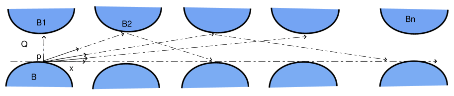
Figure 3: Periodic orbits in infinite horizon case.

Let $B^{u}(\zeta_{n})$ be the curvature of the unstable wave front, see [17, Chapter 3] for a precise definition. By time reversibility, we know that $B^{u}(\zeta_{n})=B^{u}(T\zeta_{n})$. By [17] (3.34), writing $\zeta_{n}=(0,\vartheta_{n})$,

$$B^{u}(\zeta_{n})=\frac{1}{\tau(\zeta_{n})+\frac{1}{R(\zeta_{n})+\frac{1}{B^{u}(\zeta_{n})}}}$$

where $\tau(\zeta_{n})$ is the free path of the periodic point $\zeta_{n}$, and $R(\zeta_{n})=\frac{2K(\zeta_{n})}{\cos\vartheta_{n}}$ is the collision factor, $K(\zeta_{n})$ is the curvature of the base point of $\zeta_{n}$. Solving the above equation, we get

$$B^{u}(\zeta_{n})=R(\zeta_{n})(\sqrt{1+\frac{4}{R(\zeta_{n})\tau(\zeta_{n})}}-1)$$

For large $n$, $R(\zeta_{n})\sim n$ and $\tau(\zeta_{n})\sim n$, which implies that

$$B^{u}(\zeta_{n})=\frac{2}{\tau(\zeta_{n})}+O(n^{-2})$$

By [17, Theorem 3.38],

$$\log|DT_{u}(\zeta_{n})=\frac{1}{\tau(\zeta_{n})}\int_{0}^{\tau(\zeta_{n})}B^{u}(\Phi^{t}\zeta_{n})\,dt=\frac{1}{\tau(\zeta_{n})}\log(1+B^{u}(\zeta_{n}\tau(\zeta_{n})),$$

where [17] (3.32) is used in the estimation of the last step. By the time reversibility property of billiards, $|DT_{u}^{2}(\zeta_{n})|=|DT_{u}(\zeta_{n})|^{2}$, where $DT_{u}(\zeta_{n})$ is the derivative of $T$ in the unstable direction at $\zeta_{n}$.

Let $\theta_{n}$ be the extremal index of the periodic point $\zeta_{n}$ of period $2$. Since $1-\theta_{n}=\frac{1}{|DT^{2}_{u}(\zeta_{n})|}$ we may calculate

$$1-\theta_{n} =(1+\tau(\zeta_{n})B^{u}(\zeta_{n}))^{-\frac{2}{\tau(\zeta_{n})}}$$

$$=\left(1+\tau(\zeta_{n})R(\zeta_{n})(\sqrt{1+\frac{4}{R(\zeta_{n})\tau(\zeta_{n})}}-1)\right)^{-\frac{2}{\tau(\zeta_{n})}}$$

$$=\left(1+\frac{4}{\sqrt{1+\frac{4}{R(\zeta_{n})\tau(\zeta_{n})}}+1}\right)^{-\frac{2}{\tau(\zeta_{n})}}$$

For $n$ large enough, we have

$$\theta_{n}=1-3^{-\frac{2}{\tau(\zeta_{n})}}+O(n^{-\frac{1}{n}})$$

Thus

$$\lim_{n\to\infty}\theta_{n}=0$$

. This implies that as $n$ gets larger, the extreme index of periodic point $\xi_{n}$ is decreasing.

References

- [1] P. Balint, N. Chernov and D. Dolgopyat, Limit theorems for dispersing billiards with cusps, Comm. Math. Phys., 308 (2011), 479–510.
- [2] L.A. Bunimovich, Ya. Sinai, and N. Chernov, Markov partitions for two-dimensional billiards, Russ. Math. Surv. 45 (1990), 105–152.
- [3] L.A. Bunimovich, Ya. Sinai, and N. Chernov, Statistical properties of two-dimensional hyperbolic billiards, Russ. Math. Surv. 46 (1991), 47–106.
- [4] M. Benedicks, L.S- Young, Markov extensions and decay of correlations for certain Henon maps, Asterisque 261 (2000), 13–56.
- [5] P. Bálint and S. Gouezel, Limit theorems in the stadia billiards, Comm. Math. Phys., 263 (2006), 451–512.
- [6] L. Barreira, Y. Pesin, Nonuniformly Hyperbolicity: Dynamics of Systems with Nonzero Lyapunov Exponents, Encyclopedia of Mathematics and Its Applications, Cambridge University Press, 2007.
- [7] L. A. Bunimovich, On billiards close to dispersing, Math. USSR. Sb. 23 (1974), 45–67.
- [8] N. Chernov and D. Dolgopyat, Anomalous current in periodic Lorentz gases with infinite horizon, Russ. Math. Surv. 64 (2009), 651–699.
- [9] N. Chernov, Sinai billiards under small external forces, Ann. Henri Poincaré 2:2 (2001), 197–236.
- [10] N. Chernov, Sinai billiards under small external forces II, Ann. Henri Poincare 9 (2008), 91–107.
- [11] N. Chernov and D. Dolgopyat, Galton Board: limit theorems and recurrence, J. Amer. Math. Soc. 22 (2009), 821–858.
- [12] N. Chernov, Statistical properties of piecewise smooth hyperbolic systems in high dimensions, Discr. Cont. Dynam. Syst. 5 (1999), 425–448.
- [13] N. Chernov, G. Eyink, J. Lebowitz and Ya. Sinai, Derivation of Ohm’s law in a deterministic mechanical model, Phys. Rev. Lett. 70 (1993), 2209–2212.
- [14] N. Chernov, G. Eyink, J. Lebowitz and Ya. Sinai, Steady-state electrical conduction in the periodic Lorentz gas, Comm. Math. Phys. 154 (1993), 569–601.
- [15] N. I. Chernov and D. Dolgopyat, Hyperbolic billiards and statistical physics, Proceedings of International Congress of Mathematicians, 2006.
- [16] N. I. Chernov and D. Dolgopyat, Anomalous current in periodic Lorentz gases with an infinite horizon. Usp. Mat. Nauk 64, 73 124 (2009). (Russian), translation in Russian Math. Surveys 64, 651 699 (2009)
- [17] N. Chernov and R. Markarian, Chaotic billiards, Math. Surv. Monographs, 127, AMS, Providence, RI (2006), 316 pp.
- [18] N. Chernov and R. Markarian, Dispersing billiards with cusps: slow decay of correlations, Commun. Math. Phys., 270 (2007), 727–758.
- [19] N. Chernov and H.-K. Zhang, Billiards with polynomial mixing rates, Nonlineartity, 4 (2005), 1527–1553.
- [20] N. Chernov and H.-K. Zhang, A family of chaotic billiards with variable mixing rates, Stochast. Dynam. 5 (2005), 535–553.
- [21] N. Chernov and H.-K. Zhang, Improved estimates for correlations in billiards, Comm. Math. Phys., 277, 2008, 305–321.
- [22] N. Chernov and H.-K. Zhang, On statistical properties of hyperbolic systems with singularities, J. Stat. Phys., 136 (2009), 615–642.
- [23] J.-R. Chazottes and P. Collet. Poisson approximation for the number of visits to balls in non-uniformly hyperbolic dynamical systems. Ergodic Theory Dynamical Systems. 33 (2013), 49-80.
- [24] P. Collet. Statistics of closest return for some non-uniformly hyperbolic systems. Erg. Th. Dyn. Syst. 21 (2001), 401-420.
- [25] M.F. Demers, H.-K. Zhang, A functional analytic approach to perturbations of the Lorentz gas, Commun. Math. Phys, 2013.
- [26] M. Denker, M. Gordin, and A. Sharova. A Poisson limit theorem for toral automorphisms. Illinois J. Math, 48(1), (2004),1-20.
- [27] A. Ferguson and M. Pollicott. Escape Rates for Gibbs measures, Ergodic Theory and Dynamical Systems, 32 (2012), no. 3, 961-988.
- [28] J. Freitas, A. Freitas and M. Todd. Hitting Times and Extreme Value Theory, Probab. Theory Related Fields,147(3):675–710, 2010.
- [29] A.C.M. Freitas, J.M. Freitas, and M. Todd. Extremal Index, Hitting Time Statistics and periodicity, Adv. Math., 231, no. 5, 2012, 2626-2665.
- [30] A. C. M. Freitas, J. M. Freitas, and M. Todd. The compound Poisson limit ruling periodic extreme behaviour of non-uniformly hyperbolic dynamics. Comm. Math. Phys., 321(2), (2013), 483-527.
- [31] N. Haydn, J. Freitas and M. Nicol, Convergence of rare events point processes to the Poisson for billiards, Nonlinearity, 27, (2014) 1669-1687.
- [32] N. Haydn and S. Vaienti. The compound Poisson distribution and return times in dynamical systems. Probab. Theory Related Fields 144, (2009), no. 3-4, 517-542.
- [33] N. T. A. Hadyn and K. Wasilewska. Limiting distribution and error terms for the number of visits to balls in non-uniformly hyperbolic dynamical systems. Preprint 2015.
- [34] M. Hirata. Poisson Limit Law for Axiom A diffeomorphisms. Erg. Th. Dyn. Syst. 13 (1993), no. 3, 533–556.
- [35] M.P. Holland, M. Nicol and A. Török. Extreme value distributions for non-uniformly expanding dynamical systems. Trans. Amer. Math. Soc., 364, (2012), 661-688.
- [36] M. Carvalho, A. C. M. Freitas, J. M. Freitas, M. Holland and M. Nicol. Extremal dichotomy for hyperbolic toral automorphisms, Dynamical Systems: An International Journal Volume 30, No. 4, (2015), 383-403.
- [37] C. Gupta. Extreme-value distributions for some classes of non-uniformly partially hyperbolic dynamical systems. Ergodic Theory and Dynamical Systems, 30, (3), (2011), 757-771.
- [38] C. Gupta, M. P. Holland and M. Nicol. Extreme value theory for dispersing billiards, Lozi maps and Lorenz maps. Ergodic Theory and Dynamical Systems, 31, (5), (2011), 1363-1390.
- [39] C. Gupta, M. Holland and M. Nicol, Extreme value theory and return time statistics for dispersing billiard maps and flows, Lozi maps and Lorenz-like maps, Ergod. Th. Dynam. Sys. 31 (2011), 1363–1390.
- [40] M. P. Holland, and M. Nicol and A. Török, Extreme value distributions for non-uniformly hyperbolic dynamical systems, Trans. Amer. Math. Soc. 364 (2012), 661–688.
- [41] N. Haydn, M. Nicol, S. Vaienti and L. Zhang, Central limit theorems for the shrinking target problem, J. Stat. Physics 153 (2013), 864–887.
- [42] G. Keller. Rare events, exponential hitting times and extremal indices via spectral perturbation. Dyn. Syst. 27 (2012), no. 1, 11–27.
- [43] R. M. Loynes. Extreme values in uniformly mixing stationary stochastic processes. Ann. Math. Statist. 36, (1965), 993-999.
- [44] A. Katok, J.-M. Strelcyn, Invariant Manifolds, Entropy and Billiards; Smooth Maps with Singularities. Lect. Notes Math., 1222, Springer, New York (1986) (with the collaboration of F. Ledrappier & F. Przytycki).
- [45] Leadbetter, M. R., Lindgren, G., and Rootzen, H. (1983), Extremes and Related Properties of Random Sequences and Processes. Springer-Verlag, New York.
- [46] R. Markarian, Billiards with polynomial decay of correlations, Ergod. Th. Dyn. Syst. 24 (2004), 177–197.
- [47] F. Péne and B. Saussol. Poisson law for some nonuniformly hyperbolic dynamical systems with polynomial rate of mixing, Ergodic Theory Dynam. Systems 36 (2016), no. 8, 2602–2626.
- [48] J. Sinai. Dynamical systems with elastic reflections. Ergodic properties of dispersing billiards. (Russian), Uspehi Mat. Nauk 25 1970 no. 2 (152), 141–192.
- [49] J. Springham, R. Sturman, Polynomial decay of correlations in linked-twist maps, Ergodic Theory Dynam. Systems 34 (2014), no. 5, 1724–1746.
- [50] G. S. Watson. Extreme values in samples from m-dependent stationary stochastic processes. Ann. Math. Statist. 25, (1954), 860-863.
- [51] L.-S. Young, Statistical properties of dynamical systems with some hyperbolicity, Ann. Math. 147 (1998), 585–650.
- [52] L.-S. Young, Recurrence times and rates of mixing, Israel J. Math. 110 (1999), 153–188.
- [53] H.-K. Zhang Current in periodic Lorentz gases with twists. Commun. Math. Phys. 306 (2011), 747–776.