Semidual Kitaev lattice model and tensor network representation

Abstract

Kitaev’s lattice models are usually defined as representations of the Drinfeld quantum double $D(H)=H{\bowtie}H^{*\text{op}}$, as an example of a double cross product quantum group. We propose a new version based instead on $M(H)=H^{\text{cop}}{\blacktriangleright\!\!\!\triangleleft}H$ as an example of Majid’s bicrossproduct quantum group, related by semidualisation or ‘quantum Born reciprocity’ to $D(H)$. Given a finite-dimensional Hopf algebra $H$, we show that a quadrangulated oriented surface defines a representation of the bicrossproduct quantum group $H^{\text{cop}}{\blacktriangleright\!\!\!\triangleleft}H$. Even though the bicrossproduct has a more complicated and entangled coproduct, the construction of this new model is relatively natural as it relies on the use of the covariant Hopf algebra actions. Working locally, we obtain an exactly solvable Hamiltonian for the model and provide a definition of the ground state in terms of a tensor network representation.

1 Introduction

1.1 Motivations

The Kitaev quantum double models AYK were originally proposed to exploit topological phases of matter for fault-tolerant quantum computation. The models are based on quantum many-body systems exhibiting topological order. Their physics is obtained from Topological quantum field theories (TQFTs), while their underlying mathematical structure is based on Hopf algebras. For a given finite group $G$, Kitaev constructed an ‘extended’ Hilbert space on a triangulated oriented surface $\Sigma$ and an exactly solvable Hamiltonian, whose ground state or protected space is a topological invariant of the surface. It turns out that this triangulation or graph defines a representation of the Drinfeld quantum double $D(G)$. A well known example of these models is the Kitaev toric code, which is based on the cyclic group $\mbox{${\mathbb{Z}}$}_{2}$ AYK . See also Delgago2d3d for a recent account. It was anticipated in AYK that these models could be generalized to be based on a finite-dimensional Hopf algebra $H$. This was achieved in BMCA . Other models in the family of topologically ordered spin models such as the Levin-Wen string-net models Levin04 ; Levin06 which are based on a representation category of $H$ are also related to the Kitaev models Oliver09 ; Kadar08 . In particular, for a fusion category of representations of finite groups, a Fourier transformation of the Kitaev models lead to the extended string-net models Oliver09 ; Kadar09 ; Buerschaper2010 . The structure of excitations for these models is also well established KitaevKong ; Lan14 ; Hu18 . One defines the so called ribbon operators on the Hilbert space that generate the excitations.

The Kitaev quantum double models can be understood to describe the moduli space of flat connections on a 2d surface with defect excitations. From the point of view of quantum gravity, they are of strong interest as they are directly related to certain 3d TQFTs defined in terms of (quasitriangular) Hopf algebras. It is known that the protected space of a Kitaev model for a finite-dimensional semisimple Hopf algebra $H$ on an oriented surface $\Sigma$ is exactly the vector space that the Turaev-Viro TQFTs BW96 ; Turaev92 for the representation category of $H$ assigns to $\Sigma$ Balsam12 ; Kadar09 ; Kadar08 ; Koenig10 . The construction of these models is also closely related to BF theory with defects Delcamp16 ; Clememt16 ; Bianca16 ; Horowitz89 ; JBaez95 , a TQFT describing locally flat connections. Other recent examples include a dual picture which was introduced in the quantum gravity setting where the excitations have been swapped Dupuis:2017otn . Even though this was discovered independently, this result could have been guessed in light of the notion of electro-magnetic duality well known in topological quantum computing Buerschaper2010 . A recent paper by Meusburger show that Kitaev’s model for a finite-dimensional semisimple Hopf algebra $H$ is equivalent to the combinatorial quantization of Chern-Simons theory for the Drinfeld double $D(H)$ CM . This emerges in a gauge theoretic framework, in which both models are viewed as Hopf algebra-valued lattice gauge theories MW .

These results have opened new perspectives on the relations between topological quantum information(TQI) and quantum gravity. Although each framework comes with its own motivation, they share similar mathematical concepts. For example, in the case of TQI cases, one deals with a (ribbon) graph decorated by Hopf algebra elements and constructs an exactly solvable Hamiltonian defined in terms of operators acting on the nodes and faces of the graph. The vacuum state of this can be interpreted from the quantum gravity perspective as the pure gravity case, whereas the excitations of the TQI Hamiltonian, used to perform quantum computations, are interpreted as particles with mass or spin depending on their location. In the case of loop quantum gravity, one has torsion excitations on the nodes, i.e. spin, whereas on the faces, one has curvature excitations, i.e. mass. The most relevant algebraic structure to deal with representations which classify particles for example and indicate their braiding, is not only the Hopf algebra $H$ but the associated Drinfeld double $D(H)$. Once again, this structure was identified using different arguments in each of the different frameworks. In the TQI case, one deals with the Drinfeld’s quantum double of finite dimensional (semisimple) Hopf algebras (e.g. built from finite groups) AYK ; BombinDeldado ; BMCA whereas in the quantum gravity case one makes use of the quantum double of Hopf algebras built from Lie groups or their quantum deformation AGSI ; AGSII ; AS ; Schroers ; Freidel:2004vi ; BNR ; MeusburgerSchroers1 ; MeusburgerSchroers2 ; MN ; noui2006three ; SchroersReview .

As described above, the Drinfeld quantum double is in a sense the common quantum group which arise in the quantum computing setting. However, from the point of view of quantum gravity, other quantum groups emerge. In particular, the bicrossproduct quantum group originally proposed by Majid SM as a new foundation for quantum gravity. The bicrossproduct quantum groups are interpreted here as algebras of observables of quantum systems so that one can view them as functions on a quantum phase space. These bicrossproduct quantum groups are also known to be valid candidates for the combinatorial quantization of Chern-Simons theory of 3d gravity cath-bernd ; OseiSchroers1 ; prince-bernd ; PKO1 . In particular, from the point of view of quantum group theory, the quantum double $D(H)=H{\bowtie}H^{*\text{op}}$ is an example of a double cross product of Hopf algebras SM . It turns out that these are related to the bicrossproduct ones by Majid’s idea of semidualisation or ‘quantum Born reciprocity’, proposed for quantum gravity where one can exchange position and momentum degrees of freedom in an algebraic framework Ma:pla . The semidual partner of the quantum double here is the ‘mirror product’ $M(H)=H^{\text{cop}}{\blacktriangleright\!\!\!\triangleleft}H$, so this is the natural candidate for a ‘semidual Kitaev model’ which we propose here. It is also known that the two quantum groups are related by a Drinfeld twist if $H$ is factorisable. This was originally introduced in Majid94 as an algebraic Wick rotation, and recently applied in MO to relate the bicrossproduct model quantum spacetime Majid:1994cy and the fuzzy $\mbox{${\mathbb{R}}$}^{3}$ quantum spacetime by a module algebra twist as well as to find the universal $R$-matrix from the former model.

From the above considerations, while the bicrossproduct quantum groups emerge in a quantum gravity framework, they are yet to be explored for the topological quantum computation models. There is no general framework for the latter for general double crossproduct and nor at the moment will we find one for general bicrossproducts. However, the most important examble is the quantum double and we will see that it is possible to construct lattice quantum computation models for the case of the bicrossproduct corresponding to this.

Our consideration in the present paper will be local, i.e effectively an infinite square lattice, with topological aspects needed to apply these results to the quadrangulation or other cellular decomposition of a general oriented connected surface $\Sigma$ to be considered elsewhere.

1.2 General features of the Kitaev model

We first recall the set up for the standard Kitaev model based on the double $D(H)$ but in a manner general enough to also apply to $M(H).$ In both cases the data we really need is a quantum group $D$ acting on an algebra $A$ (so the latter is a $D$-module algebra in quantum group parlance). In 3D quantum gravity, $D$ could be the quantum Poincaé group acting on quantum spacetime $A$, which is then interpreted mathematically as a module algebra. We also need that $D$ factorises as an algebra into two subalgebras, $H_{1},H_{2}$, which are each Hopf algebras but not necessarily sub-Hopf algebras. Thus each element of $D$ can be written in the form $\sum_{i}a_{i}b_{i}$ for $a_{i}\in H_{1}$ and $b_{i}\in H_{2}$ uniquely in a certain tensor sense SM . The restriction of the action of $D$ to each subalgebra gives ‘triangle operators’ $T_{+}^{a},L^{h}_{+}$ respectively for their action on $A$.

It is convenient to suppose that $A$ is itself a Hopf algebra and we then define

$$T^{a}_{-}=S\circ T^{a}_{+}\circ S^{-1},\quad L^{h}_{-}=S\circ L^{h}_{+}\circ S^{-1}$$ (1)

using its antipode.

In the case of the double $D(H)$, the triangle operators $T_{\pm}^{a},L^{h}_{\pm}$ make $A$ respectively a $H_{1}$ module algebra and a $H_{2}$ module coalgebra. We choose to keep these features as a general property of the Kitaev model.

Now let $\Gamma$ be a graph embedded in an orientable Riemann surface $\Sigma$ and define a Hilbert space $H_{\Gamma}=A^{\mathop{\otimes}|E|}$ where $E$ are the edges of the graph. On this we define operators $A^{h}(v,p),B^{a}(v,p)$ associated to each vertex $v$ and adjacent face $p$ as follows. First of all, the edges around $v$ and $p$ are both numbered in line with the orientation and prescribed starting point. If all the edges at $v$ point in then $A^{h}(v,p)$ is the tensor product action of $h\in D$ (which uses its coproduct and the $L_{+}$ on each such edge). If some of them point out then we use $L_{-}$ on those edges. Similarly, $B^{a}(v,p)$ is the tensor product action of $a\in D$ if all the adjacent edges to $p$ are clockwise (using the coproduct and $T_{+}$). If some of them are anticlockwise, we use $T_{-}$ on those. These conventions are depicted in Figure 1.

Figure 1: Kitaev convention for triangle operators acting on an edge.

Other edges in $H_{\Gamma}$ are unaffected by $A^{h}(v,p)$ and $B^{a}(v,p).$ We will then let $a,h$ be integral elements to obtain ‘vertex and face’ operators $A_{v}$ and $B_{p}$. Details will be given in Section 3.

The standard Kitaev model based on the quantum double has $D=D(H)=H{\bowtie}H^{*\text{op}}$ acting on $A=H$, where $H$ is a finite dimensional Hopf algebra (with further properties). Here the two indicated factors are sub-Hopf algebras which makes things more straightforward. This ‘kinematic’ level of the data actually makes sense for any double cross product quantum group $H_{1}{\bowtie}H_{2}$ in the sense of SM , acting on $H_{2}^{*}$ . However, we can use the same set up for $D=M(H)=H^{\text{cop}}{\blacktriangleright\!\!\!\triangleleft}H$ acting on $A=H^{*}$, and this is what we will do. The big difference now is that $H$ here is not a sub-Hopf algebra but a quotient (there is a canonical Hopf algebra surjection $D\rightarrow H$), but it is still a subalgebra as part of an algebra cross product, so we can still dissect the action of $D$ into $T_{+},L_{+}$. We still define $T_{-},L_{-}$ in the same way for the other orientations but we must be careful in the manner stated to use the coproduct of $D$ when combining these to build $A^{h}(v,p)$ and $B^{a}(v,p).$ This much of the setup again makes sense for any bicrossproduct quantum group $H_{1}{\blacktriangleright\!\!\!\triangleleft}H_{2}$ as in SM acting on $H_{1}^{*}$. In fact the data for these models are equivalent in the finite-dimensional case – if you can build one then you can canonically build the other by a process of semidualisation SM ; Ma:pla .

In the standard case of $D(H)$, it can be shown that the associated Hamiltonian is topological, which means physically that the elementary excitations of the Kitaev model are anyons and facilitate the realisation of topological quantum computing by obeying some braid statistics AYK . The braiding is possible as a result of the quasitriangular structure or universal $R$-matrix of $D(H)$. These aspects for the $M(H)$ case will be examined elsewhere but being isomorphic to $H^{\text{cop}}\mathop{\otimes}H$ as a Hopf algebra, one has a natural canonical quasitriangular structure if $H$ does. We will however, obtain an exactly solvable Hamiltonian. Following BMCA , we then provide an explicit tensor network representation of the model. Such a representation is a starting point to explore some interesting physical properties of the system. For example in BMCA , the tensor network representation is used to probe the notion of entanglement and check whether we have an area law for entanglement entropy. It is also used to define a notion of renormalization implementing a hierarchy of states.

This completes our overview. Section 2 provides some preliminaries on Hopf algebras notations, the bicrossproduct quantum group $H^{\text{cop}}{\blacktriangleright\!\!\!\triangleleft}H$ and its action on $H^{*}$. In Section 3, we provide the detailed construction of the lattice representation based in this data and obtain the Hamiltonian for the model. In Section 4, we define the tensor network representation for our model and provide, in particular, the realisation of the ground state in our setting. We conclude in Section 5.

2 Preliminaries

We follow the notations and conventions from the book SM . Unless otherwise specified, we work over a field $k$ of characteristic zero. A Hopf algebra or ‘quantum group’ $H$ is an algebra and a coalgebra, with a linear coproduct $\Delta:H\longrightarrow H\mathop{\otimes}H$ which is an algebra homomorphism and satisfies the coassociativity condition $(\Delta\otimes\mbox{id})\circ\Delta=(\mbox{id}\otimes\Delta)\circ\Delta$. We use Sweedler notation for the coproduct so that for all $h\in H$, $\Delta(h)=h_{{}_{\scriptscriptstyle(1)}}\otimes h_{{}_{\scriptscriptstyle(2)}}=h{}^{\scriptscriptstyle(1)}\otimes h{}^{\scriptscriptstyle(2)}$. There is also a counit ${\epsilon}:H\longrightarrow k$ and an antipode $S:H\longrightarrow H$ satisfying in particular $(Sh{}_{\scriptscriptstyle(1)})h{}_{\scriptscriptstyle(2)}=h{}_{\scriptscriptstyle(1)}Sh{}_{\scriptscriptstyle(2)}={\epsilon}(h)$ for all $h\in H$. If $H$ is finite-dimensional, then $S^{-1}$ exist. We denote by $H^{\mathop{\otimes}n}$, $n\in\mbox{${\mathbb{N}}$}$ the $n$-fold tensor product of $H$. The composition of $n$ coproducts is the map $\Delta^{(n)}:H\rightarrow H^{\mathop{\otimes}(n+1)}$ defined by $\Delta^{(n)}(h)=h_{{}_{\scriptscriptstyle(1)}}\mathop{\otimes}h_{{}_{\scriptscriptstyle(2)}}\mathop{\otimes}...\mathop{\otimes}h_{(n+1)}$. This is well defined since the coproduct is coassociative. We denote by $H^{*}$ the dual Hopf algebra with dual pairing given by the non-degenerate bilinear map $\langle\,,\,\rangle$. $H^{\text{cop}},H^{\text{op}}$ denote taking the opposite coproduct or opposite product in $H$.

An algebra $A$ is said to be an $H$-module algebra if $A$ is a left $H$-module and this action is covariant, i.e.

$$h{\triangleright}(ab)=(h{}_{\scriptscriptstyle(1)}{\triangleright}a)(h{}_{\scriptscriptstyle(2)}{\triangleright}b),\hskip 28.45274pth{\triangleright}1={\epsilon}(h),\;\;a\in A,\,h\in H,$$ (2)

where ${\triangleright}$ denotes a left action. We say that $(H,A)$ is a covariant system. We will generally prefer left actions as here but there is an analgous notion for a right module algebra by action ${\triangleleft}$. This can always be coverted to a left one of the opposite algebra by $h\triangleright a=a\triangleleft S^{-1}h$. If $H$ acts on vector spaces $V,W$ then it also acts on $V\mathop{\otimes}W$ by $h{\triangleright}(v\mathop{\otimes}w)=h{}_{\scriptscriptstyle(1)}{\triangleright}v\mathop{\otimes}h{}_{\scriptscriptstyle(2)}{\triangleright}w$ for all $h\in H$, $v\in V$ and $w\in W$.

We now turn to the construction of $M(H)=H^{\text{cop}}{\blacktriangleright\!\!\!\triangleleft}H$ from SM . This is an example of Majid’s theory of bicrossproducts $H_{1}{\triangleright\!\!\!\blacktriangleleft}H_{2}$ just as the more well-known $D(H)=H{\bowtie}H^{*\text{op}}$ is an example of his theory of double cross products $H_{1}{\bowtie}H_{2}$. We refer to SM for details, while here suffice it to say that the key difference is that in the latter case each factor acts on the vector space of the other subject to certain axioms and the coproduct is the tensor product one. By contrast, in the bicrossproduct case the $H_{2}$ factor acts on the $H_{1}$ factor as a left $H_{2}$-module algebra and results in a semidirect or cross product algebra $H_{1}{>\!\!\!\triangleleft}H_{2}$. Meanwhile the $H_{1}$ factor right coacts on the coalgebra of $H_{2}$ and results in a semidirect or cross coproduct coalgebra $H_{1}{\blacktriangleright\!\!<}H_{2}$ in Majid’s notation. The construction on the coalgebra side here is conceptually dual to the construction on the algebra side. The bicrossproduct construction adds further axioms so that the two fit together to form a quantum group, with the merged notation.

In our case, $M(H)$ is an example as follows. The left action of $H$ on $H^{\text{cop}}$ and the right coaction of $H^{\text{cop}}$ on $H$ are given respectively as

$$h\triangleright a=h_{{}_{\scriptscriptstyle(1)}}aSh_{{}_{\scriptscriptstyle(2)}},\hskip 19.91684pt\Delta_{R}h=h_{{}_{\scriptscriptstyle(2)}}\otimes h_{{}_{\scriptscriptstyle(1)}}Sh_{{}_{\scriptscriptstyle(3)}}.$$ (3)

The algebra is

$$(a\otimes h)(b\otimes g)=a(h_{{}_{\scriptscriptstyle(1)}}bSh_{{}_{\scriptscriptstyle(2)}})\otimes h_{{}_{\scriptscriptstyle(3)}}g,\hskip 14.22636pth,g\in H,\hskip 8.5359pta,b\in H^{\text{cop}}.$$ (4)

Here, $H^{\text{cop}}\mathop{\otimes}1$ and $1\mathop{\otimes}H$ appear as subalgebras but with mutual commutation relation fully determined by

$$hb:=(1\otimes h)(b\otimes 1)=(h_{{}_{\scriptscriptstyle(1)}}bSh_{{}_{\scriptscriptstyle(2)}})h_{{}_{\scriptscriptstyle(3)}},$$ (5)

where the identification $h\rightarrow 1_{H^{\text{cop}}}\otimes h$ and $b\rightarrow b\otimes 1_{H}$ are algebra morphisms. The coproduct and antipode are respectively

$$\Delta(a\otimes h)= \,a_{{}_{\scriptscriptstyle(2)}}\otimes h_{{}_{\scriptscriptstyle(2)}}\otimes a_{{}_{\scriptscriptstyle(1)}}h_{{}_{\scriptscriptstyle(1)}}Sh_{{}_{\scriptscriptstyle(3)}}\otimes h_{{}_{\scriptscriptstyle(4)}},$$ (6)

$$S(a\mathop{\otimes}h)= \,(1\mathop{\otimes}Sh{}_{\scriptscriptstyle(2)})(S(ah{}_{\scriptscriptstyle(1)}Sh{}_{\scriptscriptstyle(3)})\mathop{\otimes}1).$$ (7)

The Hopf algebra $M(H)$ acts covariantly on $H^{*\text{op}}$ from the right according to

$$\phi\triangleleft(a\otimes h)=\langle ah_{{}_{\scriptscriptstyle(1)}},\phi_{{}_{\scriptscriptstyle(1)}}\rangle\langle Sh_{{}_{\scriptscriptstyle(2)}},\phi_{{}_{\scriptscriptstyle(3)}}\rangle\phi_{{}_{\scriptscriptstyle(2)}},$$ (8)

and using the antipode (7) of $M(H)$, this gives rise to covariant left action on $H^{*}$

$$(a\otimes h)\triangleright\phi=\langle Sh_{{}_{\scriptscriptstyle(1)}}Sa,\phi_{{}_{\scriptscriptstyle(1)}}\rangle\langle h_{{}_{\scriptscriptstyle(2)}},\phi_{{}_{\scriptscriptstyle(3)}}\rangle\phi_{{}_{\scriptscriptstyle(2)}}.$$ (9)

We refer to SM and to the recent work MO for more details.

3 Semidual Kitaev model

In this section, we construct a lattice representation based on the mirror bicrossproduct $H^{\text{cop}}{\blacktriangleright\!\!\!\triangleleft}H$ acting on $H^{*}$ and obtain an exactly solvable Hamiltonian for the model.

Since we consider only the local quadrangulation of a $2$d oriented surface, we effectively work with $\Gamma$ a square lattice, without worrying about boundaries or the topology of the surface. We denote by $V,E,F$ respectively the set of vertices, edges, faces of the graph $\Gamma$. Given a finite-dimensional Hopf algebra $H$ with dual $H^{*}$, we define the extended Hilbert space $\mathcal{H}_{\Gamma}$ for the model by assigning $H^{*}$ to each edge of $\Gamma$ so that

$$\mathcal{H}_{{\Gamma}}=\bigotimes_{e\in\Gamma}H^{*},$$

the $|E|$-fold tensor product of $H^{*}$ with each copy assigned to an edge of $\Gamma$. We identify $\phi\mapsto S(\phi)$, $\phi\in H^{*}$ if the orientation is reversed. Since $H^{*}$ is finite-dimensional, $S^{2}={\rm id}$ and this isomorphism is well defined.

3.1 Triangle operators

To each edge $e\in E$, we assign a family of basic linear operators $(L^{h}_{\pm})_{e}$, $(T^{a}_{\pm})_{e}$ which are linear maps on the copy of $A=H^{*}$ in the Hilbert space $H_{\Gamma}=H^{*\mathop{\otimes}|E|}$ associated to edge $e$, indexed by elements of the Hopf algebras $H$ and $H^{\text{cop}}$ respectively. They act trivially on the copies associated to other edges. These operators are called triangle operators AYK and are defined as follows:

Definition 3.1.

Let $H$ be a finite-dimensional Hopf algebra and $\Gamma$ a graph with cyclic ordering of edge ends at each vertex. Let $h\in H$, $\phi\in H^{*}$ and $a\in H^{\text{cop}}$. The triangle operators for an edge $e\in E$ are linear maps

$$(L^{h}_{\pm})_{e}:H^{*\mathop{\otimes}|E|}\rightarrow H^{*\mathop{\otimes}|E|},\quad(T^{a}_{\pm})_{e}:H^{*\mathop{\otimes}|E|}\rightarrow H^{*\mathop{\otimes}|E|},$$

where $L^{h}_{+},T^{a}_{+}:H^{*}\rightarrow H^{*}$ acting on the copy associated to $e$ are given by

$$L^{h}_{+}(\phi) = \langle h,S\phi{}_{\scriptscriptstyle(1)}\phi{}_{\scriptscriptstyle(3)}\rangle\phi{}_{\scriptscriptstyle(2)},\hskip 19.91684ptL^{h}_{-}(\phi)=\langle h,\phi{}_{\scriptscriptstyle(3)}S^{-1}\phi{}_{\scriptscriptstyle(1)}\rangle\phi{}_{\scriptscriptstyle(2)},$$

$$T^{a}_{+}(\phi) = \langle Sa,\phi{}_{\scriptscriptstyle(1)}\rangle\phi{}_{\scriptscriptstyle(2)},\hskip 51.21504ptT^{a}_{-}(\phi)=\langle a,\phi{}_{\scriptscriptstyle(2)}\rangle\phi{}_{\scriptscriptstyle(1)}.$$ (10)

Here, the operators $L_{+}$ and $T_{+}$ are the restrictions to $1\mathop{\otimes}h$ and $a\mathop{\otimes}1$ of the canonical left action (9) of the bicrossproduct $M(H)$ on $H^{*}$. The $L_{-}$ and $T_{-}$ are also left actions obtained using the relations

$${L^{h}_{-}(\phi)=(S\circ L^{h}_{+}\circ S^{-1})(\phi),\quad T^{a}_{-}(\phi)=(S\circ T^{a}_{+}\circ S^{-1})(\phi).}$$ (11)

Next, we denote by $\rho^{a\mathop{\otimes}h}_{+}=T^{a}_{+}L^{h}_{+}$ the full representation of $M(H)$ defined in (9). Using (11) we have $\rho^{a\mathop{\otimes}h}_{-}=T^{a}_{-}L^{h}_{-}$, i.e.,

$$\rho^{a\mathop{\otimes}h}_{-}(\phi)=\langle ah{}_{\scriptscriptstyle(1)},\phi{}_{\scriptscriptstyle(3)}\rangle\langle h{}_{\scriptscriptstyle(2)},S^{-1}\phi{}_{\scriptscriptstyle(1)}\rangle\phi{}_{\scriptscriptstyle(2)}.$$ (12)

It is interesting to note that for the bicrossproduct covariant system $(M(H),H^{*})$, the canonical left action of the Hopf algebra $H^{\text{cop}}$ on $H^{*}$ is the coregular action $T_{+}$ and makes $H^{*}$ into an $H^{\text{cop}}$-module algebra by construction while the canonical left action of the Hopf algebra $H$ on $H^{*}$ is the coadjoint action $L_{+}$ and makes $H^{*}$ an $H$-module coalgebra. This fits with the fact that the factor $H$ is not a sub-quantum group and we must use the correct (semidirect) coproduct of $M(H)$ to have $H^{*}$ covariant. In the quantum double model the covariant action of $D(H)$ on $H$ does not define $L_{\pm},T_{\pm}$ because they do not lead to a graph representation of $D(H)$. In the $D(H)$ Kitaev lattice model, one has a $D$ module not a $D$ module algebra.

3.2 Geometric operators

Next, the triangle operators are used to define vertex and face operators $A^{h}(v,p)$ and $B^{a}(v,p)$ for the bicrossproduct model on the extended Hilbert space $\mathcal{H}_{{\Gamma}}$. These operators are also called geometric operators. Both operators depend on a pair of vertex and face that are adjacent to each other. They require linear ordering of edges at each vertex and in each face. This is specified by a site AYK $s=(v,p)$, which consist of a face $p$ and adjacent vertex $v$ and represented by dotted lines as shown in Figure 2. Both vertices and faces are oriented anti-clockwise.

In summary, the definition of $A^{h}(v,p)$ follows by assigning the coproduct of $h\in H$ along the edges in an anticlockwise manner taking into account the site $(v,p)$, and then the appropriate action of $h$ depending on the edge orientation. Likewise, the operator $B^{a}(v,p)$ is defined, but the edges associated to the face $p$ are assigned the coproduct of $a\in H^{\text{cop}}$ anticlockwise starting from the vertex $v$. The action of $a$ is then taking depending on whether the edge orientation is on the left or right of the face $p$.

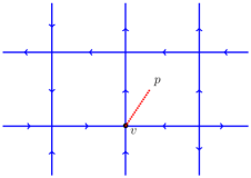
Figure 2: This figure illustrates a choice of site (the dotted line) in the graph $\Gamma$.

Definition 3.2.

Let $(v,p)$ be the site of $\Gamma$ and $h\in H$, $a\in H^{\text{cop}}$, $\phi^{i}\in H^{*}$. Let $H$ be involutive i.e., $S^{2}={\rm id}$.

• The vertex operator $A^{h}(v,p):H^{*\mathop{\otimes}|E|}\rightarrow H^{*\mathop{\otimes}|E|}$ encodes the representation of $M(H)$ at the site by

  $$A^{h}(v,p)=\rho_{\pm}^{h{}_{\scriptscriptstyle(\tilde{1})}}\mathop{\otimes}\cdots\mathop{\otimes}\rho_{\pm}^{h{}_{\scriptscriptstyle(\tilde{4})}},$$

  where $\Delta^{(3)}_{M(H)}(h)=h{{}_{\scriptscriptstyle(\tilde{1})}}\mathop{\otimes}h{{}_{\scriptscriptstyle(\tilde{2})}}\mathop{\otimes}...\mathop{\otimes}h{{}_{\scriptscriptstyle(\tilde{4})}}$ with $\Delta_{M(H)}(h)$ given by the coproduct of $M(H)$ in (6) restricted to $1\mathop{\otimes}h$. In terms of diagrams, we have

  

  where the scalar $\beta\equiv\langle h,(S\phi{}_{\scriptscriptstyle(1)}^{4})(S\phi{}_{\scriptscriptstyle(1)}^{3})(S\phi{}_{\scriptscriptstyle(1)}^{2})(S\phi{}_{\scriptscriptstyle(1)}^{1})\phi{}_{\scriptscriptstyle(3)}^{1}\phi{}_{\scriptscriptstyle(3)}^{2}\phi{}_{\scriptscriptstyle(3)}^{3}\phi{}_{\scriptscriptstyle(3)}^{4}\rangle$. The edges incident to the vertex $v$ are indexed counterclockwise starting from $p$. Here all the edges incident to the vertex $v$ are assumed to point towards $v$. Using the antipode to change orientation, we see that for edges orientated away from the vertex $v$, $\rho_{+}$ has to be replaced with $\rho_{-}$.

• The face operator $B^{a}(v,p):H^{*\mathop{\otimes}|E|}\rightarrow H^{*\mathop{\otimes}|E|}$ for the face which encodes the action of $H^{\text{cop}}$ in $M(H)$ at the site is defined by

  $$B^{a}(v,p)=T_{\pm}^{a{}_{\scriptscriptstyle(\tilde{1})}}\mathop{\otimes}\cdots\mathop{\otimes}T_{\pm}^{a{}_{\scriptscriptstyle(\tilde{4})}}$$

  where $\Delta^{(3)}_{M(H)}(a)=a{}_{\scriptscriptstyle(\tilde{1})}\mathop{\otimes}\cdots\mathop{\otimes}a{}_{\scriptscriptstyle(\tilde{4})}$ with $\Delta_{M(H)}(a)$ the coproduct of $M(H)$ (6) restricted to $a\mathop{\otimes}1$. More precisely, we have

  

We shall now show how $\Gamma$, equipped with these operators admits a local mirror bicrossproduct $M(H)$ representation at the sites of $\Gamma$. We need to show that the vertex and face operators represent their respective copies of $M(H)$ and that their commutation relations arising from common edges implement the algebra in the bicrossproduct quantum group $M(H)$.

Theorem 3.3.

Let $H$ be a finite-dimensional Hopf algebra satisfying $S^{2}={\rm id}$ with dual $H^{*}$ and the graph $\Gamma$ a square lattice as above. Then the operators $A^{h}(v,p)$ and $B^{a}(v,p)$ define an $M(H)$ representation on $H^{*\mathop{\otimes}|E|}$ associated to each site $(v,p)$. Here $(a\mathop{\otimes}h)$ acts by $A^{h}(v,p)\circ B^{a}(v,p)$, i.e. these enjoy the commutation relations

$$A^{h}(v,p)\circ B^{a}(v,p) = B^{(h{}_{\scriptscriptstyle(1)}aSh{}_{\scriptscriptstyle(2)})}(v,p)\circ A^{h{}_{\scriptscriptstyle(3)}}(v,p),\quad\forall h\in H,\;a\in H^{\text{cop}},$$ (13)

$$A^{h}(v,p)\circ A^{g}(v,p) = A^{hg}(v,p),\quad B^{a}(v,p)\circ B^{b}(v,p)=B^{ab}(v,p).$$ (14)

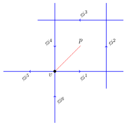
Figure 3: We illustrate here a relevant subgraph of $\Gamma$, decorated by six copies of $H^{*}$ which is the relevant structure for the proof of Theorem 3.3. Other orientations can be considered as well, but the argument follows in a similar manner. For simplicity we only focus on this graph.

Proof.

Here we only show the proof of equation (13) and leave the proof of (14) to the interested reader. Before proceeding with the proof, for the site given in Fig. 3, we note the following:

1. There are four edges connected to the vertex $v$ of Figure 3 and this requires we compute $\Delta^{(3)}$ of $M(H)$ to use in the geometric operators.

   $$\Delta^{(3)}(a\otimes h)=a{}_{\scriptscriptstyle(4)}\otimes h{}_{\scriptscriptstyle(4)}\otimes a{}_{\scriptscriptstyle(3)}h{}_{\scriptscriptstyle(3)}Sh{}_{\scriptscriptstyle(5)}\otimes h{}_{\scriptscriptstyle(6)}\otimes a{}_{\scriptscriptstyle(2)}h{}_{\scriptscriptstyle(2)}Sh{}_{\scriptscriptstyle(7)}\otimes h{}_{\scriptscriptstyle(8)}\mathop{\otimes}a{}_{\scriptscriptstyle(1)}h{}_{\scriptscriptstyle(1)}Sh{}_{\scriptscriptstyle(9)}\mathop{\otimes}h{}_{\scriptscriptstyle(10)}$$ (15)

   from which we derive that

   $$\Delta^{(3)}(a\otimes 1) = a{}_{\scriptscriptstyle(4)}\otimes 1\otimes a{}_{\scriptscriptstyle(3)}\otimes 1\otimes a{}_{\scriptscriptstyle(2)}\otimes 1\mathop{\otimes}a{}_{\scriptscriptstyle(1)}\mathop{\otimes}1$$

   $$\Delta^{(3)}(1\otimes h) = 1\otimes h{}_{\scriptscriptstyle(4)}\otimes h{}_{\scriptscriptstyle(3)}Sh{}_{\scriptscriptstyle(5)}\otimes h{}_{\scriptscriptstyle(6)}\otimes h{}_{\scriptscriptstyle(2)}Sh{}_{\scriptscriptstyle(7)}\otimes h{}_{\scriptscriptstyle(8)}\mathop{\otimes}h{}_{\scriptscriptstyle(1)}Sh{}_{\scriptscriptstyle(9)}\mathop{\otimes}h{}_{\scriptscriptstyle(10)}.$$ (16)

   These are the relevant expressions to use in the definition of the face and vertex operators.

2. The face operator associated with Figure 3 is defined as

   $$B^{a}(v,p)(\phi^{1}\otimes...\otimes\phi^{6})=T^{a{}_{\scriptscriptstyle(4)}}_{-}(\phi^{1})\mathop{\otimes}T^{a{}_{\scriptscriptstyle(3)}}_{-}(\phi^{2})\mathop{\otimes}T^{a{}_{\scriptscriptstyle(2)}}_{-}(\phi^{3})\mathop{\otimes}T^{a{}_{\scriptscriptstyle(1)}}_{-}(\phi^{4})\mathop{\otimes}\phi^{5}\mathop{\otimes}\phi^{6}$$ (17)

   and the vertex operator is

   $$A^{h}(v,p)(\phi^{1}\otimes...\otimes\phi^{6})=\rho^{h{}_{\scriptscriptstyle(\tilde{1})}}_{-}(\phi^{1})\mathop{\otimes}\phi^{2}\mathop{\otimes}\phi^{3}\mathop{\otimes}\rho^{h{}_{\scriptscriptstyle(\tilde{2})}}_{+}(\phi^{4})\mathop{\otimes}\rho^{h{}_{\scriptscriptstyle(\tilde{3})}}_{-}(\phi^{5})\mathop{\otimes}\rho^{h{}_{\scriptscriptstyle(\tilde{4})}}_{+}(\phi^{6})$$ (18)

   where $\rho_{\pm}$ are expressed in terms of the triangle operators as follows:

   $$\rho^{h{}_{\scriptscriptstyle(\tilde{1})}}_{-} \equiv \rho^{1\mathop{\otimes}h{}_{\scriptscriptstyle(4)}}_{-}=L^{h{}_{\scriptscriptstyle(4)}}_{-},\qquad\qquad\rho^{h{}_{\scriptscriptstyle(\tilde{2})}}_{+}\equiv\rho^{h{}_{\scriptscriptstyle(3)}Sh{}_{\scriptscriptstyle(5)}\otimes h{}_{\scriptscriptstyle(6)}}_{+}=T^{h{}_{\scriptscriptstyle(3)}Sh{}_{\scriptscriptstyle(5)}}_{+}L^{h{}_{\scriptscriptstyle(6)}}_{+}$$

   $$\rho^{h{}_{\scriptscriptstyle(\tilde{3})}}_{-} \equiv \rho^{h{}_{\scriptscriptstyle(2)}Sh{}_{\scriptscriptstyle(7)}\otimes h{}_{\scriptscriptstyle(8)}}_{-}=T^{h{}_{\scriptscriptstyle(2)}Sh{}_{\scriptscriptstyle(7)}}_{-}L^{h{}_{\scriptscriptstyle(8)}}_{-},\qquad\rho^{{}_{\scriptscriptstyle(\tilde{4})}}_{+}\equiv\rho^{h{}_{\scriptscriptstyle(1)}Sh{}_{\scriptscriptstyle(9)}\mathop{\otimes}h{}_{\scriptscriptstyle(10)}}_{+}=T^{h{}_{\scriptscriptstyle(1)}Sh{}_{\scriptscriptstyle(9)}}_{+}L^{h{}_{\scriptscriptstyle(10)}}_{+}.$$

   Note that $\rho_{-}$ are computed from (12). The vertex operator (18) then reads

   $$A^{h}(v,p)(\phi^{1}\otimes...\otimes\phi^{6}) = L^{h{}_{\scriptscriptstyle(4)}}_{-}(\phi^{1})\otimes\phi^{2}\mathop{\otimes}\phi^{3}\mathop{\otimes}T^{h{}_{\scriptscriptstyle(3)}Sh{}_{\scriptscriptstyle(5)}}_{+}L^{h{}_{\scriptscriptstyle(6)}}_{+}(\phi^{4})$$ (19)

   $$\,\otimes\,T^{h{}_{\scriptscriptstyle(2)}Sh{}_{\scriptscriptstyle(7)}}_{-}L^{h{}_{\scriptscriptstyle(8)}}_{-}(\phi^{5})\otimes\,T_{+}^{h{}_{\scriptscriptstyle(1)}Sh{}_{\scriptscriptstyle(9)}}L^{h{}_{\scriptscriptstyle(10)}}_{+}(\phi^{6}).$$

The proof follows a direct calculation to compare the LHS and RHS of (13). Let $h\in H$, $a\in H^{\text{cop}}$ and $\phi^{i}\in H^{*}$, where $i\in\{1,..,6\}$. Starting with the LHS of equation (13), we have

$$A^{h}(v,p)B^{a}(v,p)(\phi^{1}\otimes...\otimes\phi^{6})=A^{h}(v,p)\left(T^{a{}_{\scriptscriptstyle(4)}}_{-}(\phi^{1})\mathop{\otimes}T^{a{}_{\scriptscriptstyle(3)}}_{-}(\phi^{2})\mathop{\otimes}T^{a{}_{\scriptscriptstyle(2)}}_{-}(\phi^{3})\mathop{\otimes}T^{a{}_{\scriptscriptstyle(1)}}_{-}(\phi^{4})\mathop{\otimes}\phi^{5}\mathop{\otimes}\phi^{6}\right)$$ (20)

$$= L^{h{}_{\scriptscriptstyle(4)}}_{-}T^{a{}_{\scriptscriptstyle(4)}}_{-}(\phi^{1})\mathop{\otimes}T^{a{}_{\scriptscriptstyle(3)}}_{-}(\phi^{2})\mathop{\otimes}T^{a{}_{\scriptscriptstyle(2)}}_{-}(\phi^{3})\mathop{\otimes}T^{h{}_{\scriptscriptstyle(3)}Sh{}_{\scriptscriptstyle(5)}}_{+}L^{h{}_{\scriptscriptstyle(6)}}_{+}\left(T^{a{}_{\scriptscriptstyle(1)}}_{-}(\phi^{4})\right)$$

$$\otimes\,T^{h{}_{\scriptscriptstyle(2)}Sh{}_{\scriptscriptstyle(7)}}_{-}L^{h{}_{\scriptscriptstyle(8)}}_{-}(\phi^{5})\otimes\,T_{+}^{h{}_{\scriptscriptstyle(1)}Sh{}_{\scriptscriptstyle(9)}}L^{h{}_{\scriptscriptstyle(10)}}_{+}(\phi^{6})$$

$$= \langle a{}_{\scriptscriptstyle(4)},\phi{}_{\scriptscriptstyle(4)}^{1}\rangle\langle h{}_{\scriptscriptstyle(4)},\phi{}_{\scriptscriptstyle(3)}^{1}S^{-1}\phi{}_{\scriptscriptstyle(1)}^{1}\rangle\phi{}_{\scriptscriptstyle(2)}^{1}\mathop{\otimes}\,\langle a{}_{\scriptscriptstyle(3)},\phi{}_{\scriptscriptstyle(2)}^{2}\rangle\phi{}_{\scriptscriptstyle(1)}^{2}\mathop{\otimes}\,\langle a{}_{\scriptscriptstyle(2)},\phi{}_{\scriptscriptstyle(2)}^{3}\rangle\phi{}_{\scriptscriptstyle(1)}^{3}$$

$$\mathop{\otimes}\,\langle a{}_{\scriptscriptstyle(1)},\phi{}_{\scriptscriptstyle(6)}^{4}\rangle\langle h{}_{\scriptscriptstyle(6)},S\phi{}_{\scriptscriptstyle(1)}^{4}\phi{}_{\scriptscriptstyle(5)}^{4}\rangle\langle h{}_{\scriptscriptstyle(5)},\phi{}_{\scriptscriptstyle(2)}^{4}\rangle\langle Sh{}_{\scriptscriptstyle(3)},\phi{}_{\scriptscriptstyle(3)}^{4}\rangle\phi{}_{\scriptscriptstyle(4)}^{4}$$

$$\mathop{\otimes}\,\langle h{}_{\scriptscriptstyle(8)},\phi{}_{\scriptscriptstyle(5)}^{5}S^{-1}\phi{}_{\scriptscriptstyle(1)}^{5}\rangle\langle h{}_{\scriptscriptstyle(2)},\phi{}_{\scriptscriptstyle(3)}^{5}\rangle\langle Sh{}_{\scriptscriptstyle(7)},\phi{}_{\scriptscriptstyle(4)}^{5}\rangle\phi{}_{\scriptscriptstyle(2)}^{5}\mathop{\otimes}\,\langle h{}_{\scriptscriptstyle(10)},S\phi{}_{\scriptscriptstyle(1)}^{6}\phi{}_{\scriptscriptstyle(5)}^{6}\rangle\langle h{}_{\scriptscriptstyle(9)},\phi{}_{\scriptscriptstyle(2)}^{6}\rangle\langle Sh{}_{\scriptscriptstyle(1)},\phi{}_{\scriptscriptstyle(3)}^{6}\rangle\phi{}_{\scriptscriptstyle(4)}^{6}$$

$$= \langle a{}_{\scriptscriptstyle(4)},\phi_{{}_{\scriptscriptstyle(2)}{}_{\scriptscriptstyle(2)}}^{1}\rangle\langle h{}_{\scriptscriptstyle(4)},\phi_{{}_{\scriptscriptstyle(2)}{}_{\scriptscriptstyle(1)}}^{1}\rangle\langle S^{-1}h{}_{\scriptscriptstyle(5)},\phi_{{}_{\scriptscriptstyle(1)}{}_{\scriptscriptstyle(1)}}^{1}\rangle\phi_{{}_{\scriptscriptstyle(1)}{}_{\scriptscriptstyle(2)}}^{1}\mathop{\otimes}\,\langle a{}_{\scriptscriptstyle(3)},\phi{}_{\scriptscriptstyle(2)}^{2}\rangle\phi{}_{\scriptscriptstyle(1)}^{2}\mathop{\otimes}\,\langle a{}_{\scriptscriptstyle(2)},\phi{}_{\scriptscriptstyle(2)}^{3}\rangle\phi{}_{\scriptscriptstyle(1)}^{3}$$

$$\mathop{\otimes}\,\langle a{}_{\scriptscriptstyle(1)},\phi{}_{\scriptscriptstyle(6)}^{4}\rangle\langle h{}_{\scriptscriptstyle(6)},\phi{}_{\scriptscriptstyle(2)}^{4}\rangle\langle h{}_{\scriptscriptstyle(7)},S\phi{}_{\scriptscriptstyle(1)}^{4}\phi{}_{\scriptscriptstyle(5)}^{4}\rangle\langle Sh{}_{\scriptscriptstyle(3)},\phi{}_{\scriptscriptstyle(3)}^{4}\rangle\phi{}_{\scriptscriptstyle(4)}^{4}$$

$$\mathop{\otimes}\,\langle h{}_{\scriptscriptstyle(9)},\phi{}_{\scriptscriptstyle(5)}^{5}S^{-1}\phi{}_{\scriptscriptstyle(1)}^{5}\rangle\langle h{}_{\scriptscriptstyle(2)},\phi{}_{\scriptscriptstyle(3)}^{5}\rangle\langle h{}_{\scriptscriptstyle(8)},S\phi{}_{\scriptscriptstyle(4)}^{5}\rangle\phi{}_{\scriptscriptstyle(2)}^{5}\mathop{\otimes}\,\langle h{}_{\scriptscriptstyle(11)},S\phi{}_{\scriptscriptstyle(1)}^{6}\phi{}_{\scriptscriptstyle(5)}^{6}\rangle\langle h{}_{\scriptscriptstyle(10)},\phi{}_{\scriptscriptstyle(2)}^{6}\rangle\langle Sh{}_{\scriptscriptstyle(1)},\phi{}_{\scriptscriptstyle(3)}^{6}\rangle\phi{}_{\scriptscriptstyle(4)}^{6}$$

$$= \langle a{}_{\scriptscriptstyle(4)},\phi{}_{\scriptscriptstyle(3)}^{1}\rangle\langle S^{-1}h{}_{\scriptscriptstyle(5)}h{}_{\scriptscriptstyle(4)},\phi{}_{\scriptscriptstyle(1)}^{1}\rangle\phi{}_{\scriptscriptstyle(2)}^{1}\mathop{\otimes}\,\langle a{}_{\scriptscriptstyle(3)},\phi{}_{\scriptscriptstyle(2)}^{2}\rangle\phi{}_{\scriptscriptstyle(1)}^{2}\mathop{\otimes}\,\langle a{}_{\scriptscriptstyle(2)},\phi{}_{\scriptscriptstyle(2)}^{3}\rangle\phi{}_{\scriptscriptstyle(1)}^{3}$$

$$\mathop{\otimes}\,\langle a{}_{\scriptscriptstyle(1)},\phi{}_{\scriptscriptstyle(6)}^{4}\rangle\langle h{}_{\scriptscriptstyle(6)},\phi{}_{\scriptscriptstyle(2)}^{4}S\phi{}_{\scriptscriptstyle(1)}^{4}\phi{}_{\scriptscriptstyle(5)}^{4}\rangle\langle Sh{}_{\scriptscriptstyle(3)},\phi{}_{\scriptscriptstyle(3)}^{4}\rangle\phi{}_{\scriptscriptstyle(4)}^{4}$$

$$\mathop{\otimes}\,\langle h{}_{\scriptscriptstyle(2)},\phi{}_{\scriptscriptstyle(3)}^{5}\rangle\langle h{}_{\scriptscriptstyle(7)},S\phi{}_{\scriptscriptstyle(4)}^{5}\phi{}_{\scriptscriptstyle(5)}^{5}S^{-1}\phi{}_{\scriptscriptstyle(1)}^{5}\rangle\phi{}_{\scriptscriptstyle(2)}^{5}\mathop{\otimes}\langle h{}_{\scriptscriptstyle(8)},\phi{}_{\scriptscriptstyle(2)}^{6}S\phi{}_{\scriptscriptstyle(1)}^{6}\phi{}_{\scriptscriptstyle(5)}^{6}\rangle\langle Sh{}_{\scriptscriptstyle(1)},\phi{}_{\scriptscriptstyle(3)}^{6}\rangle\phi{}_{\scriptscriptstyle(4)}^{6}$$

$$= \langle a{}_{\scriptscriptstyle(4)},\phi{}_{\scriptscriptstyle(2)}^{1}\rangle\phi{}_{\scriptscriptstyle(1)}^{1}\epsilon(h{}_{\scriptscriptstyle(4)})\mathop{\otimes}\,\langle a{}_{\scriptscriptstyle(3)},\phi{}_{\scriptscriptstyle(2)}^{2}\rangle\phi{}_{\scriptscriptstyle(1)}^{2}\mathop{\otimes}\,\langle a{}_{\scriptscriptstyle(2)},\phi{}_{\scriptscriptstyle(2)}^{3}\rangle\phi{}_{\scriptscriptstyle(1)}^{3}\mathop{\otimes}\,\langle a{}_{\scriptscriptstyle(1)},\phi{}_{\scriptscriptstyle(4)}^{4}\rangle\langle h{}_{\scriptscriptstyle(5)},\phi{}_{\scriptscriptstyle(3)}^{4}\rangle\langle Sh{}_{\scriptscriptstyle(3)},\phi{}_{\scriptscriptstyle(1)}^{4}\rangle\phi{}_{\scriptscriptstyle(2)}^{4}$$

$$\mathop{\otimes}\,\langle h{}_{\scriptscriptstyle(2)},\phi{}_{\scriptscriptstyle(3)}^{5}\rangle\langle h{}_{\scriptscriptstyle(6)},S^{-1}\phi{}_{\scriptscriptstyle(1)}^{5}\rangle\phi{}_{\scriptscriptstyle(2)}^{5}\mathop{\otimes}\,\langle h{}_{\scriptscriptstyle(7)},\phi{}_{\scriptscriptstyle(3)}^{6}\rangle\langle Sh{}_{\scriptscriptstyle(1)},\phi{}_{\scriptscriptstyle(1)}^{6}\rangle\phi{}_{\scriptscriptstyle(2)}^{6}$$

$$= \langle a{}_{\scriptscriptstyle(4)},\phi{}_{\scriptscriptstyle(2)}^{1}\rangle\phi{}_{\scriptscriptstyle(1)}^{1}\mathop{\otimes}\,\langle a{}_{\scriptscriptstyle(3)},\phi{}_{\scriptscriptstyle(2)}^{2}\rangle\phi{}_{\scriptscriptstyle(1)}^{2}\mathop{\otimes}\,\langle a{}_{\scriptscriptstyle(2)},\phi{}_{\scriptscriptstyle(2)}^{3}\rangle\phi{}_{\scriptscriptstyle(1)}^{3}\mathop{\otimes}\,\langle a{}_{\scriptscriptstyle(1)},\phi_{{}_{\scriptscriptstyle(2)}{}_{\scriptscriptstyle(2)}}^{4}\rangle\langle h{}_{\scriptscriptstyle(4)},\phi_{{}_{\scriptscriptstyle(2)}{}_{\scriptscriptstyle(1)}}^{4}\rangle\langle Sh{}_{\scriptscriptstyle(3)},\phi_{{}_{\scriptscriptstyle(1)}{}_{\scriptscriptstyle(1)}}^{4}\rangle\phi_{{}_{\scriptscriptstyle(1)}{}_{\scriptscriptstyle(2)}}^{4}$$

$$\mathop{\otimes}\,\langle h{}_{\scriptscriptstyle(2)},\phi{}_{\scriptscriptstyle(3)}^{5}\rangle\langle h{}_{\scriptscriptstyle(5)},S^{-1}\phi{}_{\scriptscriptstyle(1)}^{5}\rangle\phi{}_{\scriptscriptstyle(2)}^{5}\mathop{\otimes}\,\langle h{}_{\scriptscriptstyle(6)},\phi{}_{\scriptscriptstyle(3)}^{6}\rangle\langle Sh{}_{\scriptscriptstyle(1)},\phi{}_{\scriptscriptstyle(1)}^{6}\rangle\phi{}_{\scriptscriptstyle(2)}^{6}$$

$$= \langle a{}_{\scriptscriptstyle(4)},\phi{}_{\scriptscriptstyle(2)}^{1}\rangle\phi{}_{\scriptscriptstyle(1)}^{1}\mathop{\otimes}\,\langle a{}_{\scriptscriptstyle(3)},\phi{}_{\scriptscriptstyle(2)}^{2}\rangle\phi{}_{\scriptscriptstyle(1)}^{2}\mathop{\otimes}\,\langle a{}_{\scriptscriptstyle(2)},\phi{}_{\scriptscriptstyle(2)}^{3}\rangle\phi{}_{\scriptscriptstyle(1)}^{3}\mathop{\otimes}\,\langle a{}_{\scriptscriptstyle(1)},\phi{}_{\scriptscriptstyle(2)}^{4}\rangle\phi{}_{\scriptscriptstyle(1)}^{4}\epsilon(h{}_{\scriptscriptstyle(3)})$$

$$\mathop{\otimes}\,\langle h{}_{\scriptscriptstyle(2)},\phi{}_{\scriptscriptstyle(3)}^{5}\rangle\langle h{}_{\scriptscriptstyle(4)},S^{-1}\phi{}_{\scriptscriptstyle(1)}^{5}\rangle\phi{}_{\scriptscriptstyle(2)}^{5}\mathop{\otimes}\,\langle h{}_{\scriptscriptstyle(5)},\phi{}_{\scriptscriptstyle(3)}^{6}\rangle\langle Sh{}_{\scriptscriptstyle(1)},\phi{}_{\scriptscriptstyle(1)}^{6}\rangle\phi{}_{\scriptscriptstyle(2)}^{6}$$

$$= \langle a,\phi{}_{\scriptscriptstyle(2)}^{1}\phi{}_{\scriptscriptstyle(2)}^{2}\phi{}_{\scriptscriptstyle(2)}^{3}\phi{}_{\scriptscriptstyle(2)}^{4}\rangle\langle h{}_{\scriptscriptstyle(2)},\phi{}_{\scriptscriptstyle(3)}^{5}\rangle\langle h{}_{\scriptscriptstyle(3)},S^{-1}\phi{}_{\scriptscriptstyle(1)}^{5}\rangle\langle Sh{}_{\scriptscriptstyle(1)},\phi{}_{\scriptscriptstyle(1)}^{6}\rangle\langle h{}_{\scriptscriptstyle(4)},\phi{}_{\scriptscriptstyle(3)}^{6}\rangle$$

$$\,\phi{}_{\scriptscriptstyle(1)}^{1}\otimes\phi{}_{\scriptscriptstyle(1)}^{2}\mathop{\otimes}\phi{}_{\scriptscriptstyle(1)}^{3}\mathop{\otimes}\phi{}_{\scriptscriptstyle(1)}^{4}\mathop{\otimes}\phi{}_{\scriptscriptstyle(2)}^{5}\mathop{\otimes}\phi{}_{\scriptscriptstyle(2)}^{6}.$$

Using the first part of (1), we calculate

$$\Delta^{3}\left(h{}_{\scriptscriptstyle(1)}aSh{}_{\scriptscriptstyle(2)}\right)=h{}_{\scriptscriptstyle(4)}a{}_{\scriptscriptstyle(4)}Sh{}_{\scriptscriptstyle(5)}\mathop{\otimes}h{}_{\scriptscriptstyle(3)}a{}_{\scriptscriptstyle(3)}Sh{}_{\scriptscriptstyle(6)}\mathop{\otimes}h{}_{\scriptscriptstyle(2)}a{}_{\scriptscriptstyle(2)}Sh{}_{\scriptscriptstyle(7)}\mathop{\otimes}h{}_{\scriptscriptstyle(1)}a{}_{\scriptscriptstyle(1)}Sh{}_{\scriptscriptstyle(8)}$$ (21)

and this will be used in computing the RHS of (13). The RHS of equation (13), is computed as follows

$$B^{h{}_{\scriptscriptstyle(1)}aSh{}_{\scriptscriptstyle(2)}}(v,p)A^{h{}_{\scriptscriptstyle(3)}}(v,p)(\phi^{1}\otimes...\otimes\phi^{6})$$ (22)

$$= B^{h{}_{\scriptscriptstyle(1)}aSh{}_{\scriptscriptstyle(2)}}(v,p)\left(L^{h{}_{\scriptscriptstyle(6)}}_{-}(\phi^{1})\otimes\phi^{2}\mathop{\otimes}\phi^{3}\mathop{\otimes}T^{h{}_{\scriptscriptstyle(5)}Sh{}_{\scriptscriptstyle(7)}}_{+}L^{h{}_{\scriptscriptstyle(8)}}_{+}(\phi^{4})\,\otimes T^{h{}_{\scriptscriptstyle(4)}Sh{}_{\scriptscriptstyle(9)}}_{-}L^{h{}_{\scriptscriptstyle(10)}}_{-}(\phi^{5})\otimes\,T_{+}^{h{}_{\scriptscriptstyle(3)}Sh{}_{\scriptscriptstyle(11)}}L^{h{}_{\scriptscriptstyle(12)}}_{+}(\phi^{6})\right)$$

$$= T^{h{}_{\scriptscriptstyle(4)}a{}_{\scriptscriptstyle(4)}Sh{}_{\scriptscriptstyle(5)}}_{-}L^{h{}_{\scriptscriptstyle(12)}}_{-}(\phi^{1})\mathop{\otimes}T^{h{}_{\scriptscriptstyle(3)}a{}_{\scriptscriptstyle(3)}Sh{}_{\scriptscriptstyle(6)}}_{-}(\phi^{2})\mathop{\otimes}T^{h{}_{\scriptscriptstyle(2)}a{}_{\scriptscriptstyle(2)}Sh{}_{\scriptscriptstyle(7)}}_{-}(\phi^{3})\mathop{\otimes}T^{h{}_{\scriptscriptstyle(1)}a{}_{\scriptscriptstyle(1)}Sh{}_{\scriptscriptstyle(8)}}_{-}T^{h{}_{\scriptscriptstyle(11)}Sh{}_{\scriptscriptstyle(13)}}_{+}L^{h{}_{\scriptscriptstyle(14)}}_{+}(\phi^{4})$$

$$\mathop{\otimes}\,T^{h{}_{\scriptscriptstyle(10)}Sh{}_{\scriptscriptstyle(15)}}_{-}L^{h{}_{\scriptscriptstyle(16)}}_{-}(\phi^{5})\mathop{\otimes}T^{h{}_{\scriptscriptstyle(9)}Sh{}_{\scriptscriptstyle(17)}}_{+}L^{h{}_{\scriptscriptstyle(18)}}_{+}(\phi^{5})$$

$$= \langle h{}_{\scriptscriptstyle(12)},\phi{}_{\scriptscriptstyle(4)}^{1}S^{-1}\phi{}_{\scriptscriptstyle(1)}^{1}\rangle\langle h{}_{\scriptscriptstyle(4)}a{}_{\scriptscriptstyle(4)}Sh{}_{\scriptscriptstyle(5)},\phi{}_{\scriptscriptstyle(3)}^{1}\rangle\phi{}_{\scriptscriptstyle(2)}^{1}\,\mathop{\otimes}\,\langle h{}_{\scriptscriptstyle(3)},\phi{}_{\scriptscriptstyle(2)}^{2}\rangle\langle a{}_{\scriptscriptstyle(3)},\phi{}_{\scriptscriptstyle(3)}^{2}\rangle\langle Sh{}_{\scriptscriptstyle(6)},\phi{}_{\scriptscriptstyle(4)}^{2}\rangle\phi{}_{\scriptscriptstyle(1)}^{2}$$

$$\mathop{\otimes}\,\langle h{}_{\scriptscriptstyle(2)},\phi{}_{\scriptscriptstyle(2)}^{3}\rangle\langle a{}_{\scriptscriptstyle(2)},\phi{}_{\scriptscriptstyle(3)}^{3}\rangle\langle Sh{}_{\scriptscriptstyle(7)},\phi{}_{\scriptscriptstyle(4)}^{3}\rangle\phi{}_{\scriptscriptstyle(1)}^{3}\,\mathop{\otimes}\,\langle h{}_{\scriptscriptstyle(14)},S\phi{}_{\scriptscriptstyle(1)}^{4}\phi{}_{\scriptscriptstyle(5)}^{4}\rangle\langle h{}_{\scriptscriptstyle(13)}Sh{}_{\scriptscriptstyle(11)},\phi{}_{\scriptscriptstyle(2)}^{4}\rangle\langle h{}_{\scriptscriptstyle(1)}a{}_{\scriptscriptstyle(1)}Sh{}_{\scriptscriptstyle(8)},\phi{}_{\scriptscriptstyle(4)}^{4}\rangle\phi{}_{\scriptscriptstyle(3)}^{4}$$

$$\mathop{\otimes}\,\langle h{}_{\scriptscriptstyle(16)},\phi{}_{\scriptscriptstyle(5)}^{5}S^{-1}\phi{}_{\scriptscriptstyle(1)}^{5}\rangle\langle h{}_{\scriptscriptstyle(10)},\phi{}_{\scriptscriptstyle(3)}^{5}\rangle\langle Sh{}_{\scriptscriptstyle(15)},\phi{}_{\scriptscriptstyle(4)}^{5}\rangle\phi{}_{\scriptscriptstyle(2)}^{5}\,\mathop{\otimes}\,\langle h{}_{\scriptscriptstyle(18)},S\phi{}_{\scriptscriptstyle(1)}^{6}\phi{}_{\scriptscriptstyle(5)}^{6}\rangle\langle h{}_{\scriptscriptstyle(17)},\phi{}_{\scriptscriptstyle(2)}^{6}\rangle\langle Sh{}_{\scriptscriptstyle(9)},\phi{}_{\scriptscriptstyle(3)}^{6}\rangle\phi{}_{\scriptscriptstyle(4)}^{6}$$

$$= \langle h{}_{\scriptscriptstyle(12)},\phi{}_{\scriptscriptstyle(4)}^{1}S^{-1}\phi{}_{\scriptscriptstyle(1)}^{1}\rangle\langle h{}_{\scriptscriptstyle(4)}a{}_{\scriptscriptstyle(4)}Sh{}_{\scriptscriptstyle(5)},\phi{}_{\scriptscriptstyle(3)}^{1}\rangle\phi{}_{\scriptscriptstyle(2)}^{1}\,\mathop{\otimes}\,\langle h{}_{\scriptscriptstyle(3)},\phi{}_{\scriptscriptstyle(2)}^{2}\rangle\langle a{}_{\scriptscriptstyle(3)},\phi{}_{\scriptscriptstyle(3)}^{2}\rangle\langle Sh{}_{\scriptscriptstyle(6)},\phi{}_{\scriptscriptstyle(4)}^{2}\rangle\phi{}_{\scriptscriptstyle(1)}^{2}$$

$$\mathop{\otimes}\,\langle h{}_{\scriptscriptstyle(2)},\phi{}_{\scriptscriptstyle(2)}^{3}\rangle\langle a{}_{\scriptscriptstyle(2)},\phi{}_{\scriptscriptstyle(3)}^{3}\rangle\langle Sh{}_{\scriptscriptstyle(7)},\phi{}_{\scriptscriptstyle(4)}^{3}\rangle\phi{}_{\scriptscriptstyle(1)}^{3}\,\mathop{\otimes}\,\langle h{}_{\scriptscriptstyle(14)},S\phi{}_{\scriptscriptstyle(1)}^{4}\phi{}_{\scriptscriptstyle(5)}^{4}\rangle\langle h{}_{\scriptscriptstyle(13)}Sh{}_{\scriptscriptstyle(11)},\phi{}_{\scriptscriptstyle(2)}^{4}\rangle\langle h{}_{\scriptscriptstyle(1)}a{}_{\scriptscriptstyle(1)}Sh{}_{\scriptscriptstyle(8)},\phi{}_{\scriptscriptstyle(4)}^{4}\rangle\phi{}_{\scriptscriptstyle(3)}^{4}$$

$$\mathop{\otimes}\,\langle h{}_{\scriptscriptstyle(15)},S\phi{}_{\scriptscriptstyle(4)}^{5}\rangle\langle h{}_{\scriptscriptstyle(16)},\phi{}_{\scriptscriptstyle(5)}^{5}S^{-1}\phi{}_{\scriptscriptstyle(1)}^{5}\rangle\langle h{}_{\scriptscriptstyle(10)},\phi{}_{\scriptscriptstyle(3)}^{5}\rangle\phi{}_{\scriptscriptstyle(2)}^{5}\,\mathop{\otimes}\,\langle h{}_{\scriptscriptstyle(17)},\phi{}_{\scriptscriptstyle(2)}^{6}\rangle\langle h{}_{\scriptscriptstyle(18)},S\phi{}_{\scriptscriptstyle(1)}^{6}\phi{}_{\scriptscriptstyle(5)}^{6}\rangle\langle Sh{}_{\scriptscriptstyle(9)},\phi{}_{\scriptscriptstyle(3)}^{6}\rangle\phi{}_{\scriptscriptstyle(4)}^{6}$$

$$= \langle h{}_{\scriptscriptstyle(12)},(\phi{}_{\scriptscriptstyle(2)}^{1}){}_{\scriptscriptstyle(2)}(S^{-1}\phi{}_{\scriptscriptstyle(1)}^{1}){}_{\scriptscriptstyle(2)}\rangle\langle h{}_{\scriptscriptstyle(4)}a{}_{\scriptscriptstyle(4)}Sh{}_{\scriptscriptstyle(5)},(\phi{}_{\scriptscriptstyle(2)}^{1}){}_{\scriptscriptstyle(1)}\rangle S(S^{-1}\phi{}_{\scriptscriptstyle(1)}^{1}){}_{\scriptscriptstyle(1)}\,\mathop{\otimes}\,\langle h{}_{\scriptscriptstyle(3)},\phi{}_{\scriptscriptstyle(2)}^{2}\rangle\langle a{}_{\scriptscriptstyle(3)},\phi{}_{\scriptscriptstyle(3)}^{2}\rangle\langle Sh{}_{\scriptscriptstyle(6)},\phi{}_{\scriptscriptstyle(4)}^{2}\rangle\phi{}_{\scriptscriptstyle(1)}^{2}$$

$$\mathop{\otimes}\,\langle h{}_{\scriptscriptstyle(2)},\phi{}_{\scriptscriptstyle(2)}^{3}\rangle\langle a{}_{\scriptscriptstyle(2)},\phi{}_{\scriptscriptstyle(3)}^{3}\rangle\langle Sh{}_{\scriptscriptstyle(7)},\phi{}_{\scriptscriptstyle(4)}^{3}\rangle\phi{}_{\scriptscriptstyle(1)}^{3}\,\mathop{\otimes}\,\langle h{}_{\scriptscriptstyle(13)},\phi{}_{\scriptscriptstyle(4)}^{4}\rangle\langle Sh{}_{\scriptscriptstyle(11)},\phi{}_{\scriptscriptstyle(1)}^{4}\rangle\langle h{}_{\scriptscriptstyle(1)}a{}_{\scriptscriptstyle(1)}Sh{}_{\scriptscriptstyle(8)},\phi{}_{\scriptscriptstyle(3)}^{4}\rangle\phi{}_{\scriptscriptstyle(2)}^{4}$$

$$\mathop{\otimes}\,\langle h{}_{\scriptscriptstyle(14)},S^{-1}\phi{}_{\scriptscriptstyle(1)}^{5}\rangle\langle h{}_{\scriptscriptstyle(10)},\phi{}_{\scriptscriptstyle(3)}^{5}\rangle\phi{}_{\scriptscriptstyle(2)}^{5}\,\mathop{\otimes}\,\langle h{}_{\scriptscriptstyle(15)},\phi{}_{\scriptscriptstyle(3)}^{6}\rangle\langle Sh{}_{\scriptscriptstyle(9)},\phi{}_{\scriptscriptstyle(1)}^{6}\rangle\phi{}_{\scriptscriptstyle(2)}^{6}$$

$$= \langle h{}_{\scriptscriptstyle(12)},(\phi{}_{\scriptscriptstyle(2)}^{1}){}_{\scriptscriptstyle(2)}(S^{-1}\phi{}_{\scriptscriptstyle(1)}^{1}){}_{\scriptscriptstyle(2)}\rangle\langle h{}_{\scriptscriptstyle(4)}a{}_{\scriptscriptstyle(4)}Sh{}_{\scriptscriptstyle(5)},(\phi{}_{\scriptscriptstyle(2)}^{1}){}_{\scriptscriptstyle(1)}\rangle S(S^{-1}\phi{}_{\scriptscriptstyle(1)}^{1}){}_{\scriptscriptstyle(1)}\,\mathop{\otimes}\,\langle h{}_{\scriptscriptstyle(3)},\phi{}_{\scriptscriptstyle(2)}^{2}\rangle\langle a{}_{\scriptscriptstyle(3)},\phi{}_{\scriptscriptstyle(3)}^{2}\rangle\langle Sh{}_{\scriptscriptstyle(6)},\phi{}_{\scriptscriptstyle(4)}^{2}\rangle\phi{}_{\scriptscriptstyle(1)}^{2}$$

$$\mathop{\otimes}\,\langle h{}_{\scriptscriptstyle(2)},\phi{}_{\scriptscriptstyle(2)}^{3}\rangle\langle a{}_{\scriptscriptstyle(2)},\phi{}_{\scriptscriptstyle(3)}^{3}\rangle\langle Sh{}_{\scriptscriptstyle(7)},\phi{}_{\scriptscriptstyle(4)}^{3}\rangle\phi{}_{\scriptscriptstyle(1)}^{3}\,\mathop{\otimes}\,\langle h{}_{\scriptscriptstyle(13)},\phi{}_{\scriptscriptstyle(4)}^{4}\rangle\langle Sh{}_{\scriptscriptstyle(11)},\phi{}_{\scriptscriptstyle(1)}^{4}\rangle\langle h{}_{\scriptscriptstyle(1)}a{}_{\scriptscriptstyle(1)}Sh{}_{\scriptscriptstyle(8)},\phi{}_{\scriptscriptstyle(3)}^{4}\rangle\phi{}_{\scriptscriptstyle(2)}^{4}$$

$$\mathop{\otimes}\,\langle h{}_{\scriptscriptstyle(14)},S^{-1}\phi{}_{\scriptscriptstyle(1)}^{5}\rangle\langle h{}_{\scriptscriptstyle(10)},\phi{}_{\scriptscriptstyle(3)}^{5}\rangle\phi{}_{\scriptscriptstyle(2)}^{5}\,\mathop{\otimes}\,\langle h{}_{\scriptscriptstyle(15)},\phi{}_{\scriptscriptstyle(3)}^{6}\rangle\langle Sh{}_{\scriptscriptstyle(9)},\phi{}_{\scriptscriptstyle(1)}^{6}\rangle\phi{}_{\scriptscriptstyle(2)}^{6}$$

$$= \langle h{}_{\scriptscriptstyle(4)}a{}_{\scriptscriptstyle(4)}Sh{}_{\scriptscriptstyle(5)},\phi{}_{\scriptscriptstyle(2)}^{1}\rangle\phi{}_{\scriptscriptstyle(1)}^{1}\,\mathop{\otimes}\,\langle h{}_{\scriptscriptstyle(3)},\phi{}_{\scriptscriptstyle(2)}^{2}\rangle\langle a{}_{\scriptscriptstyle(3)},\phi{}_{\scriptscriptstyle(3)}^{2}\rangle\langle Sh{}_{\scriptscriptstyle(6)},\phi{}_{\scriptscriptstyle(4)}^{2}\rangle\phi{}_{\scriptscriptstyle(1)}^{2}$$

$$\mathop{\otimes}\,\langle h{}_{\scriptscriptstyle(2)},\phi{}_{\scriptscriptstyle(2)}^{3}\rangle\langle a{}_{\scriptscriptstyle(2)},\phi{}_{\scriptscriptstyle(3)}^{3}\rangle\langle Sh{}_{\scriptscriptstyle(7)},\phi{}_{\scriptscriptstyle(4)}^{3}\rangle\phi{}_{\scriptscriptstyle(1)}^{3}\,\mathop{\otimes}\,\langle h{}_{\scriptscriptstyle(12)},\phi{}_{\scriptscriptstyle(4)}^{4}\rangle\langle Sh{}_{\scriptscriptstyle(11)},\phi{}_{\scriptscriptstyle(1)}^{4}\rangle\langle h{}_{\scriptscriptstyle(1)}a{}_{\scriptscriptstyle(1)}Sh{}_{\scriptscriptstyle(8)},\phi{}_{\scriptscriptstyle(3)}^{4}\rangle\phi{}_{\scriptscriptstyle(2)}^{4}$$

$$\mathop{\otimes}\,\langle h{}_{\scriptscriptstyle(13)},S^{-1}\phi{}_{\scriptscriptstyle(1)}^{5}\rangle\langle h{}_{\scriptscriptstyle(10)},\phi{}_{\scriptscriptstyle(3)}^{5}\rangle\phi{}_{\scriptscriptstyle(2)}^{5}\,\mathop{\otimes}\,\langle h{}_{\scriptscriptstyle(14)},\phi{}_{\scriptscriptstyle(3)}^{6}\rangle\langle Sh{}_{\scriptscriptstyle(9)},\phi{}_{\scriptscriptstyle(1)}^{6}\rangle\phi{}_{\scriptscriptstyle(2)}^{6}$$

$$= \langle h{}_{\scriptscriptstyle(4)},\phi_{{}_{\scriptscriptstyle(1)}{}_{\scriptscriptstyle(2)}}^{1}\rangle\langle a{}_{\scriptscriptstyle(4)},\phi_{{}_{\scriptscriptstyle(2)}{}_{\scriptscriptstyle(1)}}^{1}\rangle\langle Sh{}_{\scriptscriptstyle(5)},\phi_{{}_{\scriptscriptstyle(2)}{}_{\scriptscriptstyle(2)}}^{1}\rangle\phi_{{}_{\scriptscriptstyle(1)}{}_{\scriptscriptstyle(1)}}^{1}\,\mathop{\otimes}\,\langle h{}_{\scriptscriptstyle(3)},\phi{}_{\scriptscriptstyle(2)}^{2}\rangle\langle a{}_{\scriptscriptstyle(3)},\phi{}_{\scriptscriptstyle(3)}^{2}\rangle\langle Sh{}_{\scriptscriptstyle(6)},\phi{}_{\scriptscriptstyle(4)}^{2}\rangle\phi{}_{\scriptscriptstyle(1)}^{2}$$

$$\mathop{\otimes}\,\langle h{}_{\scriptscriptstyle(2)},\phi{}_{\scriptscriptstyle(2)}^{3}\rangle\langle a{}_{\scriptscriptstyle(2)},\phi{}_{\scriptscriptstyle(3)}^{3}\rangle\langle Sh{}_{\scriptscriptstyle(7)},\phi{}_{\scriptscriptstyle(4)}^{3}\rangle\phi{}_{\scriptscriptstyle(1)}^{3}\,\mathop{\otimes}\,\langle h{}_{\scriptscriptstyle(12)},\phi{}_{\scriptscriptstyle(4)}^{4}\rangle\langle Sh{}_{\scriptscriptstyle(11)},\phi{}_{\scriptscriptstyle(1)}^{4}\rangle\langle h{}_{\scriptscriptstyle(1)}a{}_{\scriptscriptstyle(1)}Sh{}_{\scriptscriptstyle(8)},\phi{}_{\scriptscriptstyle(3)}^{4}\rangle\phi{}_{\scriptscriptstyle(2)}^{4}$$

$$\mathop{\otimes}\,\langle h{}_{\scriptscriptstyle(13)},S^{-1}\phi{}_{\scriptscriptstyle(1)}^{5}\rangle\langle h{}_{\scriptscriptstyle(10)},\phi{}_{\scriptscriptstyle(3)}^{5}\rangle\phi{}_{\scriptscriptstyle(2)}^{5}\,\mathop{\otimes}\,\langle h{}_{\scriptscriptstyle(14)},\phi{}_{\scriptscriptstyle(3)}^{6}\rangle\langle Sh{}_{\scriptscriptstyle(9)},\phi{}_{\scriptscriptstyle(1)}^{6}\rangle\phi{}_{\scriptscriptstyle(2)}^{6}$$

$$= \langle a{}_{\scriptscriptstyle(4)},\phi{}_{\scriptscriptstyle(2)}^{1}\rangle\phi{}_{\scriptscriptstyle(1)}^{1}\,\mathop{\otimes}\,\langle h{}_{\scriptscriptstyle(3)},\phi_{{}_{\scriptscriptstyle(1)}{}_{\scriptscriptstyle(2)}}^{2}\rangle\langle a{}_{\scriptscriptstyle(3)},\phi_{{}_{\scriptscriptstyle(2)}{}_{\scriptscriptstyle(1)}}^{2}\rangle\langle Sh{}_{\scriptscriptstyle(4)},\phi_{{}_{\scriptscriptstyle(2)}{}_{\scriptscriptstyle(2)}}^{2}\rangle\phi_{{}_{\scriptscriptstyle(1)}{}_{\scriptscriptstyle(1)}}^{2}$$

$$\mathop{\otimes}\,\langle h{}_{\scriptscriptstyle(2)},\phi{}_{\scriptscriptstyle(2)}^{3}\rangle\langle a{}_{\scriptscriptstyle(2)},\phi{}_{\scriptscriptstyle(3)}^{3}\rangle\langle Sh{}_{\scriptscriptstyle(5)},\phi{}_{\scriptscriptstyle(4)}^{3}\rangle\phi{}_{\scriptscriptstyle(1)}^{3}\,\mathop{\otimes}\,\langle h{}_{\scriptscriptstyle(10)},\phi{}_{\scriptscriptstyle(4)}^{4}\rangle\langle Sh{}_{\scriptscriptstyle(9)},\phi{}_{\scriptscriptstyle(1)}^{4}\rangle\langle h{}_{\scriptscriptstyle(1)}a{}_{\scriptscriptstyle(1)}Sh{}_{\scriptscriptstyle(6)},\phi{}_{\scriptscriptstyle(3)}^{4}\rangle\phi{}_{\scriptscriptstyle(2)}^{4}$$

$$\mathop{\otimes}\,\langle h{}_{\scriptscriptstyle(11)},S^{-1}\phi{}_{\scriptscriptstyle(1)}^{5}\rangle\langle h{}_{\scriptscriptstyle(8)},\phi{}_{\scriptscriptstyle(3)}^{5}\rangle\phi{}_{\scriptscriptstyle(2)}^{5}\,\mathop{\otimes}\,\langle h{}_{\scriptscriptstyle(12)},\phi{}_{\scriptscriptstyle(3)}^{6}\rangle\langle Sh{}_{\scriptscriptstyle(7)},\phi{}_{\scriptscriptstyle(1)}^{6}\rangle\phi{}_{\scriptscriptstyle(2)}^{6}$$

$$= \langle a{}_{\scriptscriptstyle(4)},\phi{}_{\scriptscriptstyle(2)}^{1}\rangle\phi{}_{\scriptscriptstyle(1)}^{1}\,\mathop{\otimes}\,\langle a{}_{\scriptscriptstyle(3)},\phi{}_{\scriptscriptstyle(2)}^{2}\rangle\phi{}_{\scriptscriptstyle(1)}^{2}\mathop{\otimes}\,\langle a{}_{\scriptscriptstyle(2)},\phi_{{}_{\scriptscriptstyle(2)}{}_{\scriptscriptstyle(1)}}^{3}\rangle\langle h{}_{\scriptscriptstyle(2)},\phi_{{}_{\scriptscriptstyle(1)}{}_{\scriptscriptstyle(2)}}^{3}\rangle\langle Sh{}_{\scriptscriptstyle(3)},\phi_{{}_{\scriptscriptstyle(2)}{}_{\scriptscriptstyle(2)}}^{3}\rangle\phi_{{}_{\scriptscriptstyle(1)}{}_{\scriptscriptstyle(1)}}^{3}$$

$$\mathop{\otimes}\,\langle h{}_{\scriptscriptstyle(8)},\phi{}_{\scriptscriptstyle(6)}^{4}\rangle\langle Sh{}_{\scriptscriptstyle(7)},\phi{}_{\scriptscriptstyle(1)}^{4}\rangle\langle h{}_{\scriptscriptstyle(1)},\phi{}_{\scriptscriptstyle(3)}^{4}\rangle\langle a{}_{\scriptscriptstyle(1)},\phi{}_{\scriptscriptstyle(4)}^{4}\rangle\langle Sh{}_{\scriptscriptstyle(4)},\phi{}_{\scriptscriptstyle(5)}^{4}\rangle\phi{}_{\scriptscriptstyle(2)}^{4}$$

$$\mathop{\otimes}\,\langle h{}_{\scriptscriptstyle(9)},S^{-1}\phi{}_{\scriptscriptstyle(1)}^{5}\rangle\langle h{}_{\scriptscriptstyle(6)},\phi{}_{\scriptscriptstyle(3)}^{5}\rangle\phi{}_{\scriptscriptstyle(2)}^{5}\,\mathop{\otimes}\,\langle h{}_{\scriptscriptstyle(10)},\phi{}_{\scriptscriptstyle(3)}^{6}\rangle\langle Sh{}_{\scriptscriptstyle(5)},\phi{}_{\scriptscriptstyle(1)}^{6}\rangle\phi{}_{\scriptscriptstyle(2)}^{6}.$$

It follows that

$$B^{h{}_{\scriptscriptstyle(1)}aSh{}_{\scriptscriptstyle(2)}}(v,p)A^{h_{{}_{\scriptscriptstyle(3)}}}(v,p)(\phi^{1}\otimes...\otimes\phi^{6})=\langle a{}_{\scriptscriptstyle(4)},\phi{}_{\scriptscriptstyle(2)}^{1}\rangle\phi{}_{\scriptscriptstyle(1)}^{1}\,\mathop{\otimes}\,\langle a{}_{\scriptscriptstyle(3)},\phi{}_{\scriptscriptstyle(2)}^{2}\rangle\phi{}_{\scriptscriptstyle(1)}^{2}\mathop{\otimes}\,\langle a{}_{\scriptscriptstyle(3)},\phi{}_{\scriptscriptstyle(2)}^{3}\rangle\phi{}_{\scriptscriptstyle(1)}^{3}$$ (23)

$$\mathop{\otimes}\,\langle a{}_{\scriptscriptstyle(1)},\phi_{{}_{\scriptscriptstyle(2)}{}_{\scriptscriptstyle(2)}}^{4}\rangle\langle h{}_{\scriptscriptstyle(6)},\phi_{{}_{\scriptscriptstyle(3)}{}_{\scriptscriptstyle(2)}}^{4}\rangle\langle Sh{}_{\scriptscriptstyle(5)},\phi_{{}_{\scriptscriptstyle(1)}{}_{\scriptscriptstyle(1)}}^{4}\rangle\langle h{}_{\scriptscriptstyle(1)},\phi_{{}_{\scriptscriptstyle(2)}{}_{\scriptscriptstyle(1)}}^{4}\rangle\langle Sh{}_{\scriptscriptstyle(2)},\phi_{{}_{\scriptscriptstyle(3)}{}_{\scriptscriptstyle(1)}}^{4}\rangle\phi_{{}_{\scriptscriptstyle(1)}{}_{\scriptscriptstyle(2)}}^{4}$$

$$\mathop{\otimes}\,\langle h{}_{\scriptscriptstyle(7)},S^{-1}\phi{}_{\scriptscriptstyle(1)}^{5}\rangle\langle h{}_{\scriptscriptstyle(4)},\phi{}_{\scriptscriptstyle(3)}^{5}\rangle\phi{}_{\scriptscriptstyle(2)}^{5}\,\mathop{\otimes}\,\langle h{}_{\scriptscriptstyle(8)},\phi{}_{\scriptscriptstyle(3)}^{6}\rangle\langle Sh{}_{\scriptscriptstyle(3)},\phi{}_{\scriptscriptstyle(1)}^{6}\rangle\phi{}_{\scriptscriptstyle(2)}^{6}$$

$$= \langle a{}_{\scriptscriptstyle(4)},\phi{}_{\scriptscriptstyle(2)}^{1}\rangle\phi{}_{\scriptscriptstyle(1)}^{1}\,\mathop{\otimes}\,\langle a{}_{\scriptscriptstyle(3)},\phi{}_{\scriptscriptstyle(2)}^{2}\rangle\phi{}_{\scriptscriptstyle(1)}^{2}\mathop{\otimes}\,\langle a{}_{\scriptscriptstyle(3)},\phi{}_{\scriptscriptstyle(2)}^{3}\rangle\phi{}_{\scriptscriptstyle(1)}^{3}\,\mathop{\otimes}\,\langle a{}_{\scriptscriptstyle(1)},\phi{}_{\scriptscriptstyle(3)}^{3}\rangle\langle h{}_{\scriptscriptstyle(4)},\phi{}_{\scriptscriptstyle(4)}^{4}\rangle\langle Sh{}_{\scriptscriptstyle(3)},\phi{}_{\scriptscriptstyle(1)}^{4}\rangle\phi{}_{\scriptscriptstyle(2)}^{4}$$

$$\mathop{\otimes}\,\langle h{}_{\scriptscriptstyle(5)},S^{-1}\phi{}_{\scriptscriptstyle(1)}^{5}\rangle\langle h{}_{\scriptscriptstyle(2)},\phi{}_{\scriptscriptstyle(3)}^{5}\rangle\phi{}_{\scriptscriptstyle(2)}^{5}\,\mathop{\otimes}\,\langle h{}_{\scriptscriptstyle(6)},\phi{}_{\scriptscriptstyle(3)}^{6}\rangle\langle Sh{}_{\scriptscriptstyle(1)},\phi{}_{\scriptscriptstyle(1)}^{6}\rangle\phi{}_{\scriptscriptstyle(2)}^{6}$$

$$= \langle a{}_{\scriptscriptstyle(4)},\phi{}_{\scriptscriptstyle(2)}^{1}\rangle\phi{}_{\scriptscriptstyle(1)}^{1}\,\mathop{\otimes}\,\langle a{}_{\scriptscriptstyle(3)},\phi{}_{\scriptscriptstyle(2)}^{2}\rangle\phi{}_{\scriptscriptstyle(1)}^{2}\mathop{\otimes}\,\langle a{}_{\scriptscriptstyle(3)},\phi{}_{\scriptscriptstyle(2)}^{3}\rangle\phi{}_{\scriptscriptstyle(1)}^{3}\,\mathop{\otimes}\,\langle a{}_{\scriptscriptstyle(1)},\phi_{{}_{\scriptscriptstyle(2)}{}_{\scriptscriptstyle(1)}}^{3}\rangle\langle h{}_{\scriptscriptstyle(3)},(S\phi{}_{\scriptscriptstyle(1)}^{4}){}_{\scriptscriptstyle(2)}\phi_{{}_{\scriptscriptstyle(2)}{}_{\scriptscriptstyle(2)}}^{4}\rangle S^{-1}(S\phi{}_{\scriptscriptstyle(1)}^{4}){}_{\scriptscriptstyle(1)}$$

$$\mathop{\otimes}\,\langle h{}_{\scriptscriptstyle(4)},S^{-1}\phi{}_{\scriptscriptstyle(1)}^{5}\rangle\langle h{}_{\scriptscriptstyle(2)},\phi{}_{\scriptscriptstyle(3)}^{5}\rangle\phi{}_{\scriptscriptstyle(2)}^{5}\,\mathop{\otimes}\,\langle h{}_{\scriptscriptstyle(5)},\phi{}_{\scriptscriptstyle(3)}^{6}\rangle\langle Sh{}_{\scriptscriptstyle(1)},\phi{}_{\scriptscriptstyle(1)}^{6}\rangle\phi{}_{\scriptscriptstyle(2)}^{6}$$

$$= \langle a{}_{\scriptscriptstyle(4)},\phi{}_{\scriptscriptstyle(2)}^{1}\rangle\phi{}_{\scriptscriptstyle(1)}^{1}\,\mathop{\otimes}\,\langle a{}_{\scriptscriptstyle(3)},\phi{}_{\scriptscriptstyle(2)}^{2}\rangle\phi{}_{\scriptscriptstyle(1)}^{2}\mathop{\otimes}\,\langle a{}_{\scriptscriptstyle(3)},\phi{}_{\scriptscriptstyle(2)}^{3}\rangle\phi{}_{\scriptscriptstyle(1)}^{3}\,\mathop{\otimes}\,\langle a{}_{\scriptscriptstyle(1)},\phi{}_{\scriptscriptstyle(2)}^{3}\rangle\phi{}_{\scriptscriptstyle(1)}^{4}$$

$$\mathop{\otimes}\,\langle h{}_{\scriptscriptstyle(3)},S^{-1}\phi{}_{\scriptscriptstyle(1)}^{5}\rangle\langle h{}_{\scriptscriptstyle(2)},\phi{}_{\scriptscriptstyle(3)}^{5}\rangle\phi{}_{\scriptscriptstyle(2)}^{5}\,\mathop{\otimes}\,\langle h{}_{\scriptscriptstyle(4)},\phi{}_{\scriptscriptstyle(3)}^{6}\rangle\langle Sh{}_{\scriptscriptstyle(1)},\phi{}_{\scriptscriptstyle(1)}^{6}\rangle\phi{}_{\scriptscriptstyle(2)}^{6}$$

$$= \langle a,\phi{}_{\scriptscriptstyle(2)}^{1}\phi{}_{\scriptscriptstyle(2)}^{2}\phi{}_{\scriptscriptstyle(2)}^{3}\phi{}_{\scriptscriptstyle(2)}^{4}\rangle\langle h{}_{\scriptscriptstyle(2)},\phi{}_{\scriptscriptstyle(3)}^{5}\rangle\langle h{}_{\scriptscriptstyle(3)},S^{-1}\phi{}_{\scriptscriptstyle(1)}^{5}\rangle\langle Sh{}_{\scriptscriptstyle(1)},\phi{}_{\scriptscriptstyle(1)}^{6}\rangle\langle h{}_{\scriptscriptstyle(4)},\phi{}_{\scriptscriptstyle(3)}^{6}\rangle$$

$$\,\phi{}_{\scriptscriptstyle(1)}^{1}\otimes\phi{}_{\scriptscriptstyle(1)}^{2}\mathop{\otimes}\phi{}_{\scriptscriptstyle(1)}^{3}\mathop{\otimes}\phi{}_{\scriptscriptstyle(1)}^{4}\mathop{\otimes}\phi{}_{\scriptscriptstyle(2)}^{5}\mathop{\otimes}\phi{}_{\scriptscriptstyle(2)}^{6}.$$

Finally we see equations (20) and (23) are the same, and hence this proves Theorem 3.3 for the specific graph in 3. The variations according to different orientations proceed similarly and are omitted.

∎

When the geometric operators do not act at the same site, they essentially commute as stated in the following proposition.

Proposition 3.4.

Let $\Gamma$ be the square lattice described above, and $h,g\in H$ and $a,b\in H^{\text{cop}}$.

• For all sites, $A^{h}(v,p)\circ A^{g}(w,q)=A^{g}(w,q)\circ A^{h}(v,p)$ provided the vertices $v$ and $w$ do not coincide, i.e., $v\neq w$ and there are no edges connecting to $v$ and $w$ directly.

• For all sites, $B^{a}(v,p)\circ B^{b}(w,q)=B^{b}(w,q)\circ B^{a}(v,p)$ if the faces $p$ and $q$ do not coincide, i.e., $p\neq q$.

• At disjoint sites, $v\neq v^{\prime}$ and $p\neq p^{\prime}$, $A^{h}(v,p)\circ B^{b}(v^{\prime},p^{\prime})=B^{b}(v^{\prime},p^{\prime})\circ A^{h}(v,p)$.

Proof.

Before we prove the above proposition, we note triangle operators (3.1) obey the following commutation relations

$$[T_{+}^{a},T_{-}^{b}] = 0,\quad L^{h}_{\pm}T^{a}_{\pm}=T^{h{}_{\scriptscriptstyle(1)}aSh{}_{\scriptscriptstyle(2)}}_{\pm}L^{h{}_{\scriptscriptstyle(3)}}_{\pm},\,\text{for all}\;\;h,g\in H,\;a,b\in H^{\text{cop}}.$$ (24)

(i) Consider the two graphs in Figure 4 with vertices $v$ and $w$ which do not coincide and have no edges connecting them. Then it can be shown easily that the graph (with $p\neq q$) on the left has the following vertex operators $A^{h}(v,p)$ and $A^{g}(w,q)$ commuting. If one considers the graph (with $p=q$) on the right side of Figure 4, the vertex operators are computed as

$$A^{h}(v,p)(\phi^{1}\mathop{\otimes}\phi^{2}\mathop{\otimes}\phi^{3}\mathop{\otimes}\phi^{4}\mathop{\otimes}\psi^{1}\mathop{\otimes}\psi^{2}\mathop{\otimes}\psi^{3}\mathop{\otimes}\psi^{4})$$

$$= \langle h,(S\phi{}_{\scriptscriptstyle(1)}^{4})(S\phi{}_{\scriptscriptstyle(1)}^{3})(S\phi{}_{\scriptscriptstyle(1)}^{2})(S\phi{}_{\scriptscriptstyle(1)}^{1})\phi{}_{\scriptscriptstyle(3)}^{1}\phi{}_{\scriptscriptstyle(3)}^{2}\phi{}_{\scriptscriptstyle(3)}^{3}\phi{}_{\scriptscriptstyle(3)}^{4}\rangle\phi{}_{\scriptscriptstyle(2)}^{1}\mathop{\otimes}\phi{}_{\scriptscriptstyle(2)}^{2}\mathop{\otimes}\phi{}_{\scriptscriptstyle(2)}^{3}\mathop{\otimes}\phi{}_{\scriptscriptstyle(2)}^{4}\mathop{\otimes}\psi^{1}\mathop{\otimes}\psi^{2}\mathop{\otimes}\psi^{3}\mathop{\otimes}\psi^{4}$$

$$A^{g}(w,p)(\phi^{1}\mathop{\otimes}\phi^{2}\mathop{\otimes}\phi^{3}\mathop{\otimes}\phi^{4}\mathop{\otimes}\psi^{1}\mathop{\otimes}\psi^{2}\mathop{\otimes}\psi^{3}\mathop{\otimes}\psi^{4})$$

$$= \langle g,(S\psi{}_{\scriptscriptstyle(1)}^{4})(S\psi{}_{\scriptscriptstyle(1)}^{3})(S\psi{}_{\scriptscriptstyle(1)}^{2})(S\psi{}_{\scriptscriptstyle(1)}^{1})\psi{}_{\scriptscriptstyle(3)}^{1}\psi{}_{\scriptscriptstyle(3)}^{2}\psi{}_{\scriptscriptstyle(3)}^{3}\psi{}_{\scriptscriptstyle(3)}^{4}\rangle\phi^{1}\mathop{\otimes}\phi^{2}\mathop{\otimes}\phi^{3}\mathop{\otimes}\phi^{4}\mathop{\otimes}\psi{}_{\scriptscriptstyle(2)}^{1}\mathop{\otimes}\psi{}_{\scriptscriptstyle(2)}^{2}\mathop{\otimes}\psi{}_{\scriptscriptstyle(2)}^{3}\mathop{\otimes}\psi{}_{\scriptscriptstyle(2)}^{4}.$$

A straightforward calculation shows that the above computed vertex operators commute, essentially because the operators do not act on the same Hilbert spaces. The choice of orientation of the edges is not changing this. A similar calculation applies for the three other cases where $v$ and $w$ are diagonally opposite on the same square, and $p$ and $q$ are different.

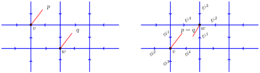
Figure 4: Diagrams showing two different graphs each with vertices $v$ and $w$ which do not coincide. We could also consider three more cases, where $v$ and $w$ are diagonally opposite and $p$ and $q$ different.

(ii) Given the graph on the right of Figure 5 with no edge(s) connecting the faces $p$ and $q$, it is easy to see that their respective face operators $B^{a}(v,p)$ and $B^{b}(w,q)$ commute. Indeed, in this case, the operators act on non-overlapping Hilbert spaces (regardless of the orientation).

Let us then assume that the face $p$ and the face $q$ share at least a common edge (with dashed line) as shown by the graph on the left of Figure 5. Then we only need to verify that the operators $B^{a}(v,p)$ and $B^{b}(w,q)$ commute on their shared edge. This common edge is oriented such that it is on the left of $p$ and on the right of $q$. Then $B^{a}(v,p)$ will acts on the edge through $T_{-}$ whiles $B^{b}(w,q)$ will acts on the edge through $T_{+}$. From (24) we know that $T_{-}$ and $T_{+}$ commute implying that the operators $B^{a}(v,p)$ and $B^{b}(w,q)$ commute also. Changing the orientation of the edges is not affecting this result.

(iii) Consider Figure 5 below with two different graphs each with disjoint sites $(v,p)$ and $(v^{\prime},p^{\prime})$. Here by disjoint sites we mean $(v,p)\neq(v^{\prime},p^{\prime})$ though common edges shared by faces $p$ and $q$ are allowed leading to $p$ and $q$ adjacent to each other as illustrated by the graph on the left of Figure 5. The second graph on the right of Figure 5 however has no edges common to both sites.

For both graphs of Figure 5 their respective vertex operator for the site $(v,p)$ moving anticlockwise are the same (changing the orientation of either graph does not change the final outcome)

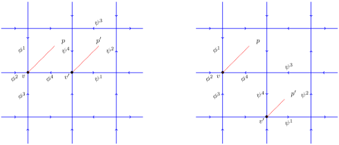
Figure 5: Diagram depicting two different graphs each with disjoint sites $(v,p)$ and $(v^{\prime},p^{\prime})$.

$$A^{h}(v,p)(\phi^{1}\mathop{\otimes}\phi^{2}\mathop{\otimes}\phi^{3}\mathop{\otimes}\phi^{4}\mathop{\otimes}\psi^{1}\mathop{\otimes}\psi^{2}\mathop{\otimes}\psi^{3}\mathop{\otimes}\psi^{4})$$

$$= L^{h{}_{\scriptscriptstyle(4)}}_{+}(\phi^{1})\mathop{\otimes}T^{h{}_{\scriptscriptstyle(3)}Sh{}_{\scriptscriptstyle(5)}}_{+}L^{h{}_{\scriptscriptstyle(6)}}_{+}(\phi^{2})\mathop{\otimes}T^{h{}_{\scriptscriptstyle(2)}Sh{}_{\scriptscriptstyle(7)}}_{+}L^{h{}_{\scriptscriptstyle(8)}}_{+}(\phi^{3})\mathop{\otimes}T^{h{}_{\scriptscriptstyle(1)}Sh{}_{\scriptscriptstyle(9)}}_{+}L^{h{}_{\scriptscriptstyle(10)}}_{+}(\phi^{4})\mathop{\otimes}\psi^{1}\mathop{\otimes}\psi^{2}\mathop{\otimes}\psi^{3}\mathop{\otimes}\psi^{4}$$

and likewise the face operator for both graphs is the same for site $(v^{\prime},p^{\prime})$ moving counterclockwise

$$B^{b}(v^{\prime},p^{\prime})(\phi^{1}\otimes\phi^{2}\mathop{\otimes}\phi^{3}\mathop{\otimes}\phi^{4}\mathop{\otimes}\psi^{1}\mathop{\otimes}\psi^{2}\mathop{\otimes}\psi^{3}\mathop{\otimes}\psi^{4})$$ (26)

$$= \phi^{1}\mathop{\otimes}\phi^{2}\mathop{\otimes}\phi^{3}\mathop{\otimes}\phi^{4}\mathop{\otimes}T^{b{}_{\scriptscriptstyle(4)}}_{-}(\psi^{1})\mathop{\otimes}T^{b{}_{\scriptscriptstyle(3)}}_{-}(\psi^{2})\mathop{\otimes}T^{b{}_{\scriptscriptstyle(2)}}_{-}(\psi^{3})\mathop{\otimes}T^{b{}_{\scriptscriptstyle(1)}}_{-}(\psi^{4}).$$

These operators commute as they act on non-overlapping Hilbert spaces. Changing the orientation of the edges would not affect this. ∎

3.3 Hilbert space and Hamiltonian

We are almost ready to define the Hamiltonian of the semidual Kitaev model. The last piece we need to define is an inner product on $H_{\Gamma}=H^{\mathop{\otimes}|E|}$ making it into a Hilbert space, and to define a self-adjoint Hamiltonian on it. To this end, we henceforth work over $k=\mbox{${\mathbb{C}}$}$ and, moreover, we suppose that $H$ is a finite- dimensional Hopf $\mbox{${\mathbb{C}}$}^{\star}$-algebra e.g. as in KLS ; NS .

To define such Hilbert space, we require $H$ be a finite-dimensional Hopf $C^{\star}$-algebra. This choice of $H$ permits for the definition of an inner product and a $\star$-representation for the model. This kind of Hopf algebra comes equipped with normalized Haar integrals, structures which are natural candidates to define an inner product. We recall that a normalised Haar integral in any Hopf algebra $H$ means $\ell\in H$ such that

$$h\cdot\ell=\ell\cdot h=\epsilon(h)\ell,\quad\text{for all }h\in H\text{ and }\epsilon(\ell)=1.$$ (27)

Moreover, in the finite dimensional Hopf $\mbox{${\mathbb{C}}$}^{\star}$ case one knows KLS ; NS that $S^{2}={\rm id}$ and there exists a unique two-sided integral $\ell\in H$ satisfying the following properties:

$$\ell^{2}=\ell,\quad\ell^{\star}=\ell,\quad S(\ell)=\ell,\quad\ell\in\text{Cocom ($H$)}.$$ (28)

Here Cocom($H$) means the flipped/opposite coproduct and the original coproduct of $H$ are the same, i.e., $\text{Cocom}(H)=\{\ell\in H|\Delta^{\text{cop}}(\ell)=\Delta(\ell)\}$.

By virtue of duality, $H^{*}$ is also a finite-dimensional Hopf $C^{\star}$-algebra. We define the extended Hilbert space $\mathcal{H}_{{\Gamma}}$ for the model by

$$\mathcal{H}_{{\Gamma}}=\bigotimes_{e\in\Gamma}H^{*},$$ (29)

where we define the tensor product inner product structure. Here the non-degenerate Hermitian inner product on each $H^{*}$ is defined by KLS ; NS

$$\langle\phi|\psi\rangle_{H^{*}}:=\langle\ell,\phi^{\star}\psi\rangle,\hskip 11.38092pt\phi,\psi\in H^{*},$$ (30)

where $\ell$ is the normalized Haar integral of $H$.

The inner product (30) allows to define the adjoint of the triangle operators $L_{\pm}$ and $T_{\pm}$

$$(L_{\pm}^{h})^{\dagger}=L_{\pm}^{h^{\star}},\qquad(T_{\pm}^{a})^{\dagger}=T_{\pm}^{a^{\star}}.$$

For example, we check this for $T_{-}^{a}$ as follows:

$$\langle\phi|T^{a}_{-}(\psi)\rangle_{H^{*}} = \langle\ell,\phi^{\star}T^{a}_{-}(\psi)\rangle=\langle\ell,\phi^{\star}\langle a,\psi{}_{\scriptscriptstyle(2)}\rangle\psi{}_{\scriptscriptstyle(1)}\rangle=\langle\ell,\langle a{}_{\scriptscriptstyle(3)},\psi{}_{\scriptscriptstyle(2)}\rangle\langle a{}_{\scriptscriptstyle(2)}Sa{}_{\scriptscriptstyle(1)},\phi{}_{\scriptscriptstyle(2)}^{*}\rangle\phi{}_{\scriptscriptstyle(1)}^{*}\psi{}_{\scriptscriptstyle(1)}\rangle$$

$$= \langle\ell,\langle a{}_{\scriptscriptstyle(3)},\psi{}_{\scriptscriptstyle(2)}\rangle\langle a{}_{\scriptscriptstyle(2)},\phi{}_{\scriptscriptstyle(2)}^{*}\rangle\langle Sa{}_{\scriptscriptstyle(1)},\phi{}_{\scriptscriptstyle(3)}^{*}\rangle\phi{}_{\scriptscriptstyle(1)}^{*}\psi{}_{\scriptscriptstyle(1)}\rangle$$

$$= \langle\ell,\langle a{}_{\scriptscriptstyle(2)},\psi{}_{\scriptscriptstyle(2)}\phi{}_{\scriptscriptstyle(2)}^{*}\rangle\langle Sa{}_{\scriptscriptstyle(1)},\phi{}_{\scriptscriptstyle(3)}^{*}\rangle\phi{}_{\scriptscriptstyle(1)}^{*}\psi{}_{\scriptscriptstyle(1)}\rangle$$

$$= \langle\ell,\langle a{}_{\scriptscriptstyle(2)},(\psi\phi{}_{\scriptscriptstyle(1)}^{*}){}_{\scriptscriptstyle(2)}\rangle\langle Sa{}_{\scriptscriptstyle(1)},\phi{}_{\scriptscriptstyle(2)}^{*}\rangle(\phi{}_{\scriptscriptstyle(1)}^{*}\psi){}_{\scriptscriptstyle(1)}\rangle$$

$$= \langle\ell,\langle a{}_{\scriptscriptstyle(2)},\phi{}_{\scriptscriptstyle(2)}^{*}\rangle\phi{}_{\scriptscriptstyle(1)}^{*}\psi\rangle=\langle T_{-}^{a^{*}}(\phi)|\psi\rangle.$$

Similarly this holds for $L_{\pm}$ and $T_{+}$. Consequently, the adjoint operators of $A^{h}$ and $B^{a}$ are respectively

$$(A^{h}(v,p))^{\dagger}=A^{h^{\star}}(v,p),\quad(B^{a}(v,p))^{\dagger}=B^{a^{\star}}(v,p).$$ (31)

We intend to build the Hamiltonian from the geometric operators. By construction, we want an Hamiltonian which is hermitian. Hence we would like to restrict the geometric operators so that they become hermitian.

One way to proceed is to use the Haar integral which will have two main advantages. First by construction $\ell^{\star}=\ell$ so it will ensure that the operators are hermitian. Second, because $\ell^{2}=\ell$, the geometric operators will become projectors. The choice of the Haar integral is in fact key in proving that the model will be topological, in the quantum double case BMCA .

Lemma 3.5.

Let $\ell\in H$, $k\in H^{\text{cop}}$ be normalized Haar integrals of the finite-dimensional Hopf $C^{\star}$-algebras $H$ and $H^{\text{cop}}$ respectively. The vertex and face operators $A^{\ell}(v,p),B^{k}(v,p):H^{*\mathop{\otimes}|E|}\rightarrow H^{*\mathop{\otimes}|E|}$ form a set of commuting Hermitian projectors.

Proof.

The proof follows directly from the properties of the Haar integral outlined in (28).

$$(A^{\ell}(v,p))^{2}=A^{\ell^{2}}(v,p)=A^{\ell}(v,p)\equiv A_{v},\quad(B^{k}(v,p))^{2}=B^{k^{2}}(v,p)=B^{k}(v,p).$$

From (13), using the properties of the Haar integrals (28), it is clear that these projectors commute. ∎

The vertex and face operators depend on the cyclic ordering of the edge ends at each vertex but no longer on the starting point one has to make. This is because the Haar integrals have the $n$-th coproduct $\Delta^{(n)}(\ell)$ invariant CM under cyclic permutations $\forall n\in\mathbb{N}$. Hence we can now shorten the notation

$$A^{\ell}(v,p)\equiv A_{v},\quad B^{k}(v,p)\equiv B_{p}.$$ (32)

We are now ready to define the Hamiltonian of the theory.

Definition 3.6.

For $\Gamma$ as above, the Hamiltonian defining the bicrossproduct $M(H)$ model on $H_{\Gamma}$ is given by

$$\hbox{{$\mathfrak{H}$}}=\sum_{v\in V}({\rm id}-A_{v})+\sum_{p\in F}({\rm id}-B_{p}).$$ (33)

The space of ground states or protected space of the Hamiltonian (33) is given by the invariant subspace $\mathcal{P}_{\Gamma}$ of $\mathfrak{H}$:

$$\mathcal{P}_{\Gamma}:=\{\phi\in\hbox{{$\mathcal{H}$}}_{{\Gamma}}:A_{v}(\phi)=\phi,\;B_{p}(\phi)=\phi,\;\forall v,p\}.$$ (34)

Since the operators $A_{v}$ and $B_{p}$ are self-adjoint, one ensures that the Hamiltonian is self-adjoint.

4 Tensor network representations for semidual models

We would like now to determine a representation of the ground state $\mathcal{P}_{\Gamma}$ of $\mathfrak{H}$. Following closely BMCA , we construct a tensor network representation of the ground state, parametrized by a graph $\Gamma$, of the mirror bicrossproduct model of Section 3. Such representation can be useful to probe the entanglement properties of the states and define some hierarchy of states as discussed in BMCA .

Our starting point is to provide the diagrammatic framework for the tensor network states built on $\Gamma$ and decorated by $H^{*}$. The construction includes graphs whose underlying surface has boundaries.

4.1 Diagrammatic scheme for tensor network states and tensor trace

Graph.

The set of edges $E$ of the graph $\Gamma$ corresponding to the surface $\Sigma$ may be decomposed into a disjoint union of interior edges and boundary edges. If due to the presence of the boundary, we have open edges, i.e., not closed faces, we can deform the graph in the appropriate way to have closed faces, as depicted in Figure 6, which we reproduce from BMCA .

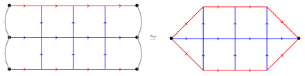
Figure 6: The interior and boundary faces of a graph. Figure reproduced from BMCA . The key-point is that some boundary faces might not be plain square plaquettes.

Forming a set consisting of the different sections of the boundary edges and faces, a natural ordering is inherited from the orientation of the boundary of the surface. For our discussion, the orientation of any boundary is fixed at an anticlockwise direction with regards to the interior of the surface.

Tensor of rank 2.

To each pair of oriented edge $e$ and face $p$, we associate a tensor of rank 2, as indicated in Figure 7.

Figure 7: The black dot represents the orientation of the edge inherited from the underlying graph. The black arrows (virtual edges) attached to the tensor represents the indices of the tensor. The association of a tensor to each edge of $\Gamma$ also amounts to placing an anti-clockwise oriented virtual loop in each face of the graph ${\Gamma}$. A virtual loop determines a face $p\in F$. This tensor has two legs hence it is seen as a tensor of rank 2.

Rank 2 tensors can be tensored to generate higher rank tensors and then contracted to follow the combinatorics of the graph $\Gamma$. They form in this case a tensor network, which is then a (complex) number since all legs are contracted, such as in Fig. 8.

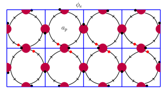
Figure 8: Example of a tensor network for a graph $\Gamma$. The reason of the presence of the red bullets will become clear in Figure 11.

The rule for contraction of the tensor network is as follows: one first splits the tensor in terms of rank 2 tensors and then contracts each pair of virtual edges separately and glue these pieces together.

Trace.

To associate a number to a given tensor network, we use the fact that an element $\phi_{e}\in H^{*}$ is associated to each edge $e\in E$ and that we can associate an element $a_{p}\in H^{\text{cop}}$ to each plaquette. We can then use the canonical pairing to associate a number to a (degenerate) decorated graph which we interpret as a trace of the tensor, as illustrated in Fig. 9, for a tensor of rank 2.

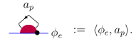
Figure 9: We consider first the simplest tensor depending on a single edge (decorated by $\phi_{e}$) bounding a single face (decorated by $a_{p}$). This can be viewed as a tensor of rank 2. The trace of the tensor is obtained by forming the virtual loop and using the canonical pairing between $H^{*}$ and $H^{cop}$. Geometrically this can be interpreted as the degenerate graph of a single edge bounding a single face.

Different orientations of graph edges and loops are related using the relevant antipode as shown in Figure 10.

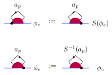
Figure 10: The different antipodes are used to change the orientation. These diagrams are assumed to be invariant under global rotations in the plane.

Contraction.

Note that while we contract tensors, it is convenient to also take the trace since at the end we are interested in the traced tensor (ie the tensor network). If the face $p$ has more edges $e$ in its boundary, we extend the diagrams in Figure 9 as follows. Consider another edge $e^{\prime}$ which shares a common vertex with $e$. We define a gluing operation as in Figure 11. Here the arrows indicate the order in which the coproduct of $a_{p}$ is applied to the basic diagrams. The red dot indicates the origin of this coproduct.

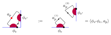
Figure 11: Gluing edges with the coproduct of $H^{\text{cop}}$.

We can keep adding edges to form a plaquette and contract the associated rank 2 tensors. Taking the trace for the final tensor is equivalent to close the virtual loop. The value of this trace is obtained by taking the product of the elements $\phi_{i}\in H^{*}$ associated to the edges.

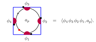
Figure 12: We keep contracting tensors of rank 2 and trace the final contraction to obtain the virtual loop and the associated number.

We note that the (red) dot on the virtual loop is important unless we deal with a co-commutative algebra $H^{\text{cop}}$. It indicates the origin of the product in $H^{*}$ which is constructed bearing in mind the $cop$ in $H^{\text{cop}}$. Furthermore, we also note that taking the trace of what looked like a degenerate graph in Figure 7 can also be interpreted as the trace of the tensor associated to the face $p$ if we have $\phi_{e}\equiv\phi_{4}\cdots\phi_{1}$. Hence as a shorthand notation for a given edge bounding a face we will sometimes use the shorthand picture displayed in Figure 13

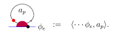
Figure 13: For a given face bounded by at most to four edges, we determine the trace of the associated rank 2 tensor. The dashed line represents the possible other red disc contributions associated to the other edges bounding the face. The $\cdots$ in the formula encodes the elements $\phi_{i}\in H^{*}$ associated to the edges bounding the face $p$. The red dot indicates that the edge we represented is the first in the (opposite) product.

Increasing the tensor rank from 2 to 4.

The edge $e$ will be in general adjacent to two faces, if there are no boundary. Hence for any edge $e$ with adjacent faces $p,q$, we pick $\phi_{e}\in H^{*}$ and $a_{p},a_{q}\in H^{\text{cop}}$ and define the face gluing operation as in Figure 14.

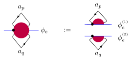
Figure 14: Gluing the faces with the coproduct of $H^{*}$, $\Delta\phi_{e}=\phi_{e}^{(1)}\otimes\phi_{e}^{(2)}$.

When the faces $p$ and $q$ have many edges, we have to put together Figure 11 and Figure 14. If furthermore one loop is outgoing we have to also consider the antipode following Figure 10.

To evaluate a pair of virtual loop $p$ and $q$, one performs a clockwise multiplication of all elements labeling the physical edges of the loop and canonically pair the result with $a_{p}$ and $a_{q}$. Graphically this is illustrated in Figure 15.

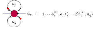
Figure 15: We denote by a dashed line the other tensor contribution for the other edges that bound the plaquette $p$. The $\cdots$ in the tensor trace denotes the contribution of these edges.

A change in the orientation of a physical edge using the antipode in $H^{*}$ changes the orientation of the corresponding tensor as shown in (35).

(35)

Trace of a tensor of arbitrary rank.

The construction of the trace extends to a general tensor.

Definition 4.1.

(Hopf tensor trace with boundaries) Let $\partial E$ and $\partial F$ be sets of boundary edges and faces respectively of $\Gamma$. The Hopf tensor trace associated with the graph ${\Gamma}$ is the function $\text{ttr}_{{\Gamma}}:H^{*\otimes|E|}\otimes H^{\text{cop}\otimes|F|}\otimes H^{*\otimes|\partial E|}\otimes H^{\text{cop}\otimes|\partial F|}\rightarrow\mathbb{C}$,

$$\bigotimes_{e\in E}\phi_{e}\bigotimes_{p\in F}a_{p}\bigotimes_{e\in\partial E}\phi^{\prime}_{e}\bigotimes_{q\in\partial F}a_{q}\longmapsto\text{ttr}_{{\Gamma}}(\{\phi_{e}\};\{a_{p}\};\{\phi^{\prime}_{e}\};\{a_{q}\})$$ (36)

which is defined via diagrams and the evaluation rules given in Figures 11, 14 and 15.

We emphasize again that our construction is very similar to the one of BMCA . Note that the Hopf tensor trace in the bicrossproduct model acts on a space dual to that of the quantum double model defined in BMCA , $(H\mathop{\otimes}H^{*\text{op}})^{*}=H^{*}\mathop{\otimes}H^{\text{cop}}$.

4.2 Quantum state

We now use the tensor trace to define quantum states for the bicrossproduct model. For simplicity we will focus on the no-boundary case.

Definition 4.2.

Let $\phi_{e}\in H^{*}$ and $a_{p}\in H^{\text{cop}}$. Let $\Gamma$ be the graph embedded in a surface $\Sigma$ with no boundaries. The Hopf tensor network state on $\Gamma$ is given by

$$|\Psi_{{\Gamma}}(\{\phi_{e}\};\{a_{p}\})\rangle:=\text{ttr}_{{\Gamma}}(\{\phi_{e}^{{}^{\scriptscriptstyle(2)}}\};\{a_{p}\})\bigotimes_{e\in E}|\phi_{e}^{{}^{\scriptscriptstyle(1)}}\rangle.$$ (37)

We shall now proceed to solve the bicrossproduct model in this framework of Hopf tensor network states. We choose a particular Hopf tensor network state as a ground state of the model so that this state is topologically ordered.

Proposition 4.3.

(Ground state of the mirror bicrossproduct model). Let $\eta$ and $k$ the Haar integrals of $H^{*}$ and $H^{\text{cop}}$ respectively. Then a ground state $|\Psi_{{\Gamma}}\rangle$ of the mirror bicrossproduct model parametrized by $\Gamma$, $|\Psi_{{\Gamma}}\rangle\in\mathcal{P}_{\Gamma}\subset\hbox{{$\mathfrak{H}$}}$ is

$$|\Psi_{{\Gamma}}\rangle:=|\Psi_{{\Gamma}}(\{\eta_{e}\};\{k_{p}\})\rangle.$$ (38)

Proof.

Recall that the Hamiltonian for the mirror bicrossproduct model is a sum of local commuting terms $A_{v}$ and $B_{p}$. Hence it is sufficient to show that the operators $A_{v}$ and $B_{p}$ leave the state $|\Psi_{{\Gamma}}\rangle$ invariant individually. To prove the proposition, it is enough to focus on the action of such operators on either a face or a vertex of the graph $\Gamma$.

A face $p$ of in the bulk of $\Gamma$ decorated by the Haar integral $k$, bounded by the four edges decorated by the Haar integral $\eta^{i}\in H^{*}$ and the four faces decorated by Haar integral $a^{i}$ leads to the contribution $|\Psi_{p}\rangle$ given by Fig. 16. Other edge/face orientations than in Fig. 16 can be treated likewise.

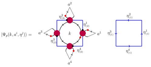
Figure 16: Contribution associated to the face $p$ to the state $\Psi_{\Gamma}$. Note that the first diagram on the right side above is the tensor trace function.

The state $|\Psi_{p}(k,a^{i},\eta^{j})\rangle$ written in an explicit form reads

$$|\Psi_{p}(k,a^{i},\eta^{j})\rangle = \langle\eta_{{}_{\scriptscriptstyle(2)}{}_{\scriptscriptstyle(2)}}^{4}\cdots\eta_{{}_{\scriptscriptstyle(2)}{}_{\scriptscriptstyle(2)}}^{1},\,k\rangle\,\prod_{j=1}^{4}\langle\cdots S\eta_{{}_{\scriptscriptstyle(2)}{}_{\scriptscriptstyle(1)}}^{j},\,a^{j}\rangle|\eta_{{}_{\scriptscriptstyle(1)}}^{1}\rangle\otimes\cdots\otimes|\eta_{{}_{\scriptscriptstyle(1)}}^{4}\rangle$$ (39)

$$= \langle\eta_{{}_{\scriptscriptstyle(3)}}^{4}\cdots\eta_{{}_{\scriptscriptstyle(3)}}^{1},\,k\rangle\prod_{j=1}^{4}\langle\cdots S\eta_{{}_{\scriptscriptstyle(2)}}^{j},\,a^{j}\rangle\,|\eta_{{}_{\scriptscriptstyle(1)}}^{1}\rangle\otimes\cdots\otimes|\eta_{{}_{\scriptscriptstyle(1)}}^{4}\rangle,$$

where the expression $\eta_{{}_{\scriptscriptstyle(3)}}^{4}\cdots\eta_{{}_{\scriptscriptstyle(3)}}^{1}$ denote composition of the elements $\eta$. We note that in the case there would be no face $j$ for example bounding $p$, we would just delete the associated $\langle S\eta_{{}_{\scriptscriptstyle(2)}}^{j},\,a^{j}\rangle$ contribution.

The state (39) is invariant under the action of $B_{p}$ as shown below

$$B^{k}_{p}|\Psi_{p}(k,a^{i},\eta^{j})\rangle = \langle\eta_{{}_{\scriptscriptstyle(3)}}^{4}\cdots\eta_{{}_{\scriptscriptstyle(3)}}^{1},\,k\rangle\langle\eta_{{}_{\scriptscriptstyle(1)}{}_{\scriptscriptstyle(1)}}^{4}\cdots\eta_{{}_{\scriptscriptstyle(1)}{}_{\scriptscriptstyle(1)}}^{1},\,k\rangle\prod_{j=1}^{4}\langle\cdots S\eta_{{}_{\scriptscriptstyle(2)}}^{j},\,a^{j}\rangle\,|\eta_{{}_{\scriptscriptstyle(1)}{}_{\scriptscriptstyle(2)}}^{1}\rangle\otimes\cdots\otimes|\eta_{{}_{\scriptscriptstyle(1)}{}_{\scriptscriptstyle(2)}}^{4}\rangle$$ (40)

$$= \langle\eta_{{}_{\scriptscriptstyle(4)}}^{4}\cdots\eta_{{}_{\scriptscriptstyle(4)}}^{1},\,k\rangle\langle\eta_{{}_{\scriptscriptstyle(1)}}^{4}\cdots\eta_{{}_{\scriptscriptstyle(1)}}^{1},\,k\rangle\prod_{j=1}^{4}\langle\cdots S\eta_{{}_{\scriptscriptstyle(3)}}^{j},\,a^{j}\rangle\,|\eta_{{}_{\scriptscriptstyle(2)}}^{1}\rangle\otimes\cdots\otimes|\eta_{{}_{\scriptscriptstyle(2)}}^{4}\rangle$$

$$= \langle\eta_{{}_{\scriptscriptstyle(3)}}^{4}\cdots\eta_{{}_{\scriptscriptstyle(3)}}^{1},\,k\rangle\langle\eta_{{}_{\scriptscriptstyle(4)}}^{4}\cdots\eta_{{}_{\scriptscriptstyle(4)}}^{1},\,k\rangle\prod_{j=1}^{4}\langle\cdots S\eta_{{}_{\scriptscriptstyle(2)}}^{j},\,a^{j}\rangle\,|\eta_{{}_{\scriptscriptstyle(1)}}^{1}\rangle\otimes\cdots\otimes|\eta_{{}_{\scriptscriptstyle(1)}}^{4}\rangle$$

$$= \langle(\eta_{{}_{\scriptscriptstyle(3)}}^{4}\cdots\eta_{{}_{\scriptscriptstyle(3)}}^{1})^{2},\,k\rangle\prod_{j=1}^{4}\langle\cdots S\eta_{{}_{\scriptscriptstyle(2)}}^{j},\,a^{j}\rangle\,|\eta_{{}_{\scriptscriptstyle(1)}}^{1}\rangle\otimes\cdots\otimes|\eta_{{}_{\scriptscriptstyle(1)}}^{4}\rangle$$

$$= \langle\eta_{{}_{\scriptscriptstyle(3)}}^{4}\cdots\eta_{{}_{\scriptscriptstyle(3)}}^{1},\,k\rangle\prod_{j}^{4}\langle\cdots S\eta_{{}_{\scriptscriptstyle(2)}}^{j},\,a^{j}\rangle\,|\eta_{{}_{\scriptscriptstyle(1)}}^{1}\rangle\otimes\cdots\otimes|\eta_{{}_{\scriptscriptstyle(1)}}^{4}\rangle$$

$$= |\Psi_{p}(k,a^{i},\eta^{j})\rangle.$$

In the first equality, we used the action of the face operator $B^{k}_{p}$ of Definition 3.2 on the state $|\Psi_{p}(k,a^{i},\eta^{j})\rangle$. We perform a renumbering on $\eta$ in the second equality. The fifth equality uses the property of the Haar integral.

Next we consider a vertex $v$ with four ingoing edges (other orientations can be treated likewise). Again, $\eta^{j}$ and $a^{i}$ are Haar integrals. The vertex contribution to $\Psi_{{\Gamma}}$ is given by Fig. 17.

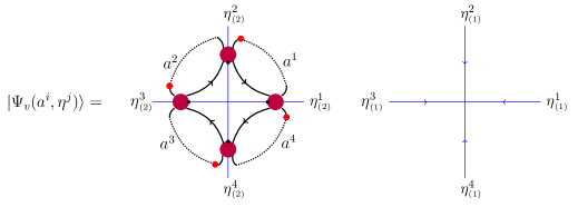
Figure 17: Contribution associated to the vertex $v$ to the state $\Psi_{\Gamma}$. Note that the first diagram on the right side above is the tensor trace function.

In a more explicit form, the state contribution from the vertex is

$$|\Psi_{v}(a^{i},\eta^{j})\rangle = \langle S\eta^{1}_{{}_{\scriptscriptstyle(2)}{}_{\scriptscriptstyle(1)}}\cdot\eta^{2}_{{}_{\scriptscriptstyle(2)}{}_{\scriptscriptstyle(2)}},\,a^{1}\rangle\cdots\langle S\eta^{4}_{{}_{\scriptscriptstyle(2)}{}_{\scriptscriptstyle(1)}}\cdot\eta^{1}_{{}_{\scriptscriptstyle(2)}{}_{\scriptscriptstyle(2)}},\,a^{4}\rangle\,|\eta_{{}_{\scriptscriptstyle(1)}}^{1}\rangle\otimes\cdots\otimes|\eta_{{}_{\scriptscriptstyle(1)}}^{4}\rangle$$ (41)

$$= \langle S\eta^{1}_{{}_{\scriptscriptstyle(2)}}\cdot\eta^{2}_{{}_{\scriptscriptstyle(3)}},\,a^{1}\rangle\cdots\langle S\eta^{3}_{{}_{\scriptscriptstyle(2)}}\cdot\eta^{4}_{{}_{\scriptscriptstyle(3)}},\,a^{4}\rangle\langle S\eta^{4}_{{}_{\scriptscriptstyle(2)}}\cdot\eta^{1}_{{}_{\scriptscriptstyle(3)}},\,a^{4}\rangle\,|\eta_{{}_{\scriptscriptstyle(1)}}^{1}\rangle\otimes\cdots\otimes|\eta_{{}_{\scriptscriptstyle(1)}}^{4}\rangle$$

$$= \prod_{j=1}^{4}\langle S\eta^{j}_{{}_{\scriptscriptstyle(2)}}\cdot\eta^{j+1}_{{}_{\scriptscriptstyle(3)}},\,a^{j}\rangle|\eta_{{}_{\scriptscriptstyle(1)}}^{1}\rangle\otimes\cdots\otimes|\eta_{{}_{\scriptscriptstyle(1)}}^{4}\rangle,$$

where if $j=4$, $j+1\equiv 1$. This convention will be used below as well. This contribution to the ground state is then invariant under the action of $A_{v}$:

$$A^{\ell}_{v}|\Psi_{v}(a^{i},\eta^{j})\rangle=\prod_{j=1}^{4}\langle S\eta^{j}_{{}_{\scriptscriptstyle(2)}}\cdot\eta^{j+1}_{{}_{\scriptscriptstyle(3)}},\,a^{j}\rangle\,\,|\eta_{{}_{\scriptscriptstyle(1)}{}_{\scriptscriptstyle(2)}}^{1}\rangle\otimes\cdots\otimes|\eta_{{}_{\scriptscriptstyle(1)}{}_{\scriptscriptstyle(2)}}^{4}\rangle$$

$$\times\,\langle\ell^{j},(S\eta^{4}_{{}_{\scriptscriptstyle(1)}{}_{\scriptscriptstyle(1)}})(S\eta^{3}_{{}_{\scriptscriptstyle(1)}{}_{\scriptscriptstyle(1)}})(S\eta^{2}_{{}_{\scriptscriptstyle(1)}{}_{\scriptscriptstyle(1)}})(S\eta^{1}_{{}_{\scriptscriptstyle(1)}{}_{\scriptscriptstyle(1)}})\eta^{1}_{{}_{\scriptscriptstyle(1)}{}_{\scriptscriptstyle(3)}}\eta^{2}_{{}_{\scriptscriptstyle(1)}{}_{\scriptscriptstyle(3)}}\eta^{3}_{{}_{\scriptscriptstyle(1)}{}_{\scriptscriptstyle(3)}}\eta^{4}_{{}_{\scriptscriptstyle(1)}{}_{\scriptscriptstyle(3)}}\rangle$$

$$= \prod_{j=1}^{4}\langle S\eta^{j}_{{}_{\scriptscriptstyle(4)}}\cdot\eta^{j+1}_{{}_{\scriptscriptstyle(3)}},\,a^{j}\rangle\,\langle\ell^{j},(S\eta{}_{\scriptscriptstyle(1)}^{4})(S\eta{}_{\scriptscriptstyle(1)}^{3})(S\eta{}_{\scriptscriptstyle(1)}^{2})(S\eta{}_{\scriptscriptstyle(1)}^{1})\eta{}_{\scriptscriptstyle(3)}^{1}\eta{}_{\scriptscriptstyle(3)}^{2}\eta{}_{\scriptscriptstyle(3)}^{3}\eta{}_{\scriptscriptstyle(3)}^{4}\rangle\,|\eta{}_{\scriptscriptstyle(2)}^{1}\rangle\otimes\cdots\otimes|\eta{}_{\scriptscriptstyle(2)}^{4}\rangle\,$$

$$= \prod_{j=1}^{4}\langle S\eta^{j}_{{}_{\scriptscriptstyle(4)}}\cdot\eta^{j+1}_{{}_{\scriptscriptstyle(3)}},\,a^{j}\rangle\langle\ell{}_{\scriptscriptstyle(1)}^{j},(S\eta{}_{\scriptscriptstyle(1)}^{4})(S\eta{}_{\scriptscriptstyle(1)}^{3})(S\eta{}_{\scriptscriptstyle(1)}^{2})(S\eta{}_{\scriptscriptstyle(1)}^{1})\rangle\langle\ell{}_{\scriptscriptstyle(2)}^{j},\eta{}_{\scriptscriptstyle(3)}^{1}\eta{}_{\scriptscriptstyle(3)}^{2}\eta{}_{\scriptscriptstyle(3)}^{3}\eta{}_{\scriptscriptstyle(3)}^{4}\rangle\,|\eta{}_{\scriptscriptstyle(2)}^{1}\rangle\otimes\cdots\otimes|\eta{}_{\scriptscriptstyle(2)}^{4}\rangle$$

$$= \prod_{j=1}^{4}\langle S\eta^{j}_{{}_{\scriptscriptstyle(4)}}\cdot\eta^{j+1}_{{}_{\scriptscriptstyle(3)}},\,a^{j}\rangle\langle S\ell{}_{\scriptscriptstyle(1)}^{j},\eta{}_{\scriptscriptstyle(1)}^{1}\eta{}_{\scriptscriptstyle(1)}^{2}\eta{}_{\scriptscriptstyle(1)}^{3}\eta{}_{\scriptscriptstyle(1)}^{4}\rangle\langle\ell{}_{\scriptscriptstyle(2)}^{j},\eta{}_{\scriptscriptstyle(3)}^{1}\eta{}_{\scriptscriptstyle(3)}^{2}\eta{}_{\scriptscriptstyle(3)}^{3}\eta{}_{\scriptscriptstyle(3)}^{4}\rangle\,|\eta{}_{\scriptscriptstyle(2)}^{1}\rangle\otimes\cdots\otimes|\eta{}_{\scriptscriptstyle(2)}^{4}\rangle$$ (42)

$$= \prod_{j=1}^{4}\langle S\eta^{j}_{{}_{\scriptscriptstyle(3)}}\cdot\eta^{j+1}_{{}_{\scriptscriptstyle(3)}},\,a^{j}\rangle\,\epsilon(\ell^{j})\,\epsilon(\eta^{1}_{{}_{\scriptscriptstyle(1)}})\,\epsilon(\eta^{2}_{{}_{\scriptscriptstyle(1)}})\,\epsilon(\eta^{3}_{{}_{\scriptscriptstyle(1)}})\,\epsilon(\eta^{4}_{{}_{\scriptscriptstyle(1)}})\,|\eta{}_{\scriptscriptstyle(2)}^{1}\rangle\otimes\cdots\otimes|\eta{}_{\scriptscriptstyle(2)}^{4}\rangle$$

$$= \prod_{j=1}^{4}\langle S\eta^{j}_{{}_{\scriptscriptstyle(2)}}\cdot\eta^{j+1}_{{}_{\scriptscriptstyle(3)}}),\,a^{j}\rangle\,|\eta{}_{\scriptscriptstyle(1)}^{1}\rangle\otimes\cdots\otimes|\eta{}_{\scriptscriptstyle(1)}^{4}\rangle=|\Psi_{v}(a^{i},\eta^{j})\rangle.$$

We used the definition of the vertex operator of Definition 3.2 in the first equality. We permute cyclicly the different components of $\eta$ in the definition of the vertex operator in the second equality. The third equality uses the counit property of a Hopf algebra. While in the fourth equality we used the fact that $\epsilon(\eta^{j}_{{}_{\scriptscriptstyle(1)}})=\epsilon(\ell^{j})=1$, to get to the fifth equality. ∎

The quantum state $|\Psi_{{\Gamma}}\rangle$ is nothing but a trivial representation of the $M(H)$ and a vacuum of the model, parametrized by $\Gamma$. If the model can be shown to be topological, which we expect it to be, such state should have then a trivial topological charge.

5 Outlook

In this article we proposed for the first time a (Kitaev) lattice model not based on the Drinfeld quantum double, but instead on the (mirror) bicrossproduct quantum group. Given a graph with cyclic ordering of edge ends at each vertex, our construction of a Hilbert space for the bicrossproduct model for a Hopf algebra $H$ is based on the extension of the canonical covariant action of the bicrossproduct quantum group $M(H)$ on $H^{*}$ to an action on $H^{*\mathop{\otimes}|E|}$, the $|E|$-fold tensor product of $H^{*}$, where $|E|$ is the number of edges. This action which enter the definition of the triangle operators and consequently the vertex and face operators are in general not required to be covariant as we seek a bicrossproduct module and not a module algebra. We obtain an exactly solvable Hamiltonian for the new model and also a representation of the ground state by introducing a tensor network representation.

As with Kitaev’s original construction AYK , which exhibited some topological features (such as the degeneracy of the ground state and the anyonic nature of quasi-particles), we suspect our model also exhibits similar topological properties. These topological features can be further explored thanks to the results in MO where the $R$-matrix – a structure known to play an important role in the braiding and fusion of quasi-particles – was explicitly given. We defer the study of the topological invariance (ie the degeneracy of the ground state) and the model properties to later investigations.

Furthermore, the physical properties of the ground state have still to be explored. In particular, thanks to the tensor network representation of the ground state we provided, it would be interesting to see whether we have some area law for the entanglement entropy, or a similar hierarchy as it was described in BMCA .

This new model opens up other new directions to explore. From the quantum gravity perspective, the vertex and face operators are related to the Gauss constraint and the Flatness constraint, which are usually characterized in terms of symmetries by the Drinfeld double in the quantum double model. It would be interesting to determine whether the bicrossproduct case has also some geometrical meaning. The semi-duality between the quantum groups seems to indicate naively that we dualize somehow for example the Flatness constraint into another Gauss constraint, or vice versa. Investigations are currently underway to see if this argument can be made more rigorous.

As the Kitaev quantum double model is known to be equivalent to the combinatorial quantization of Chern-Simons theory based on the Drinfeld double CM . It would be interesting to see whether this result extends to the bicrossproduct case, namely that our model can be related to the combinatorial quantization of Chern-Simons theory based on the bicrossproduct quantum group. In the case of the Drinfeld double, one required a Hopf gauge theoretic framework MW . This provides another interesting question to address in the context of the bicrossproduct model. For this construction, one required a universal $R$-matrix. This is now known explicitly for the bicrossproduct quantum group due to recent work in MO which provides an explicit expression of the $R$-matrix for this quantum group.

- (1) A. Yu. Kitaev, Fault tolerant quantum computation by anyons, Annals Phys. 303 (2003) 2–30, [quant-ph/9707021].
- (2) M. F. Araujo de Resende, A pedagogical overview about the 2D and 3D Toric Codes and the origin of their topological orders , 1712.01258.
- (3) O. Buerschaper, J. Martin Mombelli, M. Christandl and M. Aguado, A hierarchy of topological tensor network states, Journal of Mathematical Physics 54 (1, 2013) .
- (4) M. A. Levin and X.-G. Wen, String net condensation: A Physical mechanism for topological phases, Phys. Rev. B71 (2005) 045110, [cond-mat/0404617].
- (5) M. Levin and X.-G. Wen, Detecting Topological Order in a Ground State Wave Function, Phys. Rev. Lett. 96 (2006) 110405, [cond-mat/0510613].
- (6) O. Buerschaper and M. Aguado, Mapping Kitaev’s quantun double lattice models to Levin and Wen’s string-net models, Phys. Rev. B. 80 (2009) 115421, [cond-mat/0907.2670].
- (7) Z. Kadar, A. Marzuoli and M. Rasetti, Braiding and entanglement in spin networks: A Combinatorial approach to topological phases, in Quantum 2008: 4th Workshop Ad Memoriam of Carlo Novero: Advances in Foundations of Quantum Mechanics and Quantum Information with Atoms and Photons Turin, Italy, May 19-23, 2008, 2008, 0806.3883, http://inspirehep.net/record/789038/files/arXiv:0806.3883.pdf.
- (8) Z. Kadar, A. Marzuoli and M. Rasetti, Microscopic description of 2d topological phases, duality and 3d state sums, Adv. Math. Phys. 2010 (2010) 671039, [0907.3724].
- (9) O. Buerschaper, M. Christandl, L. Kong and M. Aguado, Electric-magnetic duality of lattice systems with topological order, Nucl. Phys. B876 (2013) 619–636, [1006.5823].
- (10) A. Kitaev and L. Kong, Models for gapped boundaries and domain walls, Commun. Math. Phys. 313 (2012) 351–373, [1104.5047].
- (11) T. Lan and X.-G. Wen, Topological quasiparticles and the holographic bulk-edge relation in (2+1) -dimensional string-net models, Phys. Rev. B90 (2014) 115119, [1311.1784].
- (12) Y. Hu, N. Geer and Y.-S. Wu, Full Dyon Excitation Spectrum in Generalized Levin-Wen Models, Phys. Rev. B97 (2018) 195154, [1502.03433].
- (13) J. W. Barrett and B. W. Westbury, Invariants of Piecewise-Linear 3-Manifolds, Trans.Amer.Math.Soc 348 (1996) 3997–4022, [hep-th/9311155].
- (14) V. G. Turaev and O. Y. Viro, State sum invariants of 3 manifolds and quantum 6j symbols, Topology 31 (1992) 865–902.
- (15) B. Balsam and A. Kirillov, Jr., Kitaev’s Lattice Model and Turaev-Viro TQFTs, 1206.2308.
- (16) R. Koenig, G. Kuperberg and R. B., Quantum computation with Turaev-Viro codes, Ann. Phys. 325 (2010) 2707–2749.
- (17) C. Delcamp, B. Dittrich and A. Riello, Fusion basis for lattice gauge theory and loop quantum gravity, JHEP 02 (2017) 061, [1607.08881].
- (18) C. Delcamp, B. Dittrich and A. Riello, On entanglement entropy in non-Abelian lattice gauge theory and 3D quantum gravity, JHEP 11 (2016) 102, [1609.04806].
- (19) C. Delcamp and B. Dittrich, From 3D topological quantum field theories to 4D models with defects, J. Math. Phys. 58 (2017) 062302, [1606.02384].
- (20) G. T. Horowitz, Exactly Soluble Diffeomorphism Invariant Theories, Commun. Math. Phys. 125 (1989) 417.
- (21) J. C. Baez, Four-Dimensional BF theory with cosmological term as a topological quantum field theory, Lett. Math. Phys. 38 (1996) 129–143, [q-alg/9507006].
- (22) M. Dupuis, L. Freidel and F. Girelli, Discretization of 3d gravity in different polarizations, Phys. Rev. D96 (2017) 086017, [1701.02439].
- (23) C. Meusburger, Kitaev lattice models as a Hopf algebra gauge theory, Commun. Math. Phys. 353 (2017) 413–468, [1607.01144].
- (24) C. Meusburger and D. K. Wise, Hopf algebra gauge theory on a ribbon graph, math.QA/1512.03966.
- (25) H. Bombin and M. A. Martin-Delgado, A Family of Non-Abelian Kitaev Models on a Lattice: Topological Confinement and Condensation, Phys. Rev. B78 (2008) 115421, [0712.0190].
- (26) A. Yu. Alekseev, H. Grosse and V. Schomerus, Combinatorial quantization of the Hamiltonian Chern-Simons theory, Commun. Math. Phys. 172 (1995) 317–358, [hep-th/9403066].
- (27) A. Yu. Alekseev, H. Grosse and V. Schomerus, Combinatorial quantization of the Hamiltonian Chern-Simons theory. 2., Commun. Math. Phys. 174 (1995) 561–604, [hep-th/9408097].
- (28) A. Yu. Alekseev and V. Schomerus, Representation theory of Chern-Simons observables, q-alg/9503016.
- (29) B. J. Schroers, Combinatorial quantization of Euclidean gravity in three dimensions, in In *Oberwolfach 1999, Quantization of singular symplectic quoti ents* 307-327, pp. 307–327, 2000, math/0006228.
- (30) L. Freidel and D. Louapre, Ponzano-Regge model revisited I: Gauge fixing, observables and interacting spinning particles, Class. Quant. Grav. 21 (2004) 5685–5726, [hep-th/0401076].
- (31) E. Buffenoir, K. Noui and P. Roche, Hamiltonian quantization of Chern-Simons theory with SL(2,C) group, Class. Quant. Grav. 19 (2002) 4953, [hep-th/0202121].
- (32) C. Meusburger and B. J. Schroers, Poisson structure and symmetry in the Chern-Simons formulation of (2+1)-dimensional gravity, Class. Quant. Grav. 20 (2003) 2193–2234, [gr-qc/0301108].
- (33) C. Meusburger and B. J. Schroers, The quantisation of Poisson structures arising inChern-Simons theory with gauge group , Adv. Theor. Math. Phys. 7 (2003) 1003–1043, [hep-th/0310218].
- (34) C. Meusburger and K. Noui, The Hilbert space of 3d gravity: quantum group symmetries and observables, Adv. Theor. Math. Phys. 14 (2010) 1651–1715, [0809.2875].
- (35) K. Noui, Three dimensional Loop Quantum Gravity: Towards a self-gravitating Quantum Field Theory, Class. Quant. Grav. 24 (2007) 329–360, [gr-qc/0612145].
- (36) B. J. Schroers, Quantum gravity and non-commutative spacetimes in three dimensions: a unified approach, Acta Phys. Polon. Supp. 4 (2011) 379–402, [1105.3945].
- (37) S. Majid, Foundations of quantum group theory. Cambridge University Press, 2011.
- (38) C. Meusburger and B. J. Schroers, Generalised Chern-Simons actions for 3d gravity and kappa-Poincare symmetry, Nucl. Phys. B806 (2009) 462–488, [0805.3318].
- (39) P. K. Osei and B. J. Schroers, On the semiduals of local isometry groups in 3d gravity, J. Math. Phys. 53 (2012) 073510, [1109.4086].
- (40) P. K. Osei and B. J. Schroers, Classical r-matrices for the generalised Chern-Simons formulation of 3d gravity, hep-th/1708.07650.
- (41) P. K. Osei, Quantum isometry groups and Born reciprocity in 3d gravity, in Physical and Mathematical Aspects of Symmetries: Proceedings of the 31st International Colloquium in Group Theoretical Methods in Physics, pp. 279–286, 2017, DOI.
- (42) S. Majid, Hopf Algebras for Physics at the Planck Scale, Class. Quant. Grav. 5 (1988) 1587–1606.
- (43) S. Majid, q Euclidean space and quantum group wick rotation by twisting, J. Math. Phys. 35 (1994) 5025–5034, [hep-th/9401112].
- (44) S. Majid and P. K. Osei, Quasitriangular structure and twisting of the 3D bicrossproduct model, JHEP 01 (2018) 147, [1708.07999].
- (45) S. Majid and H. Ruegg, Bicrossproduct structure of kappa Poincare group and noncommutative geometry, Phys. Lett. B 334 (1994) 348–354, [hep-th/9405107].
- (46) V. Kodiyalam, Z. Landau and V. Sunder, The planar algebra associated to a kac algebra, Proc. Indian Acad. Sci. Math. Sci 113 (2003) 15–51.
- (47) F. Nill and K. Szlachanyi, Quantum chains of Hopf algebras with quantum double cosymmetry, Commun. Math. Phys. 187 (1997) 159–200, [hep-th/9509100].