Fundamental work cost of quantum processes

Abstract

Information-theoretic approaches provide a promising avenue for extending the laws of thermodynamics to the nanoscale. Here, we provide a general fundamental lower limit, valid for systems with an arbitrary Hamiltonian and in contact with any thermodynamic bath, on the work cost for the implementation of any logical process. This limit is given by a new information measure—the coherent relative entropy—which accounts for the Gibbs weight of each microstate. The coherent relative entropy enjoys a collection of natural properties justifying its interpretation as a measure of information, and can be understood as a generalization of a quantum relative entropy difference. As an application, we show that the standard first and second laws of thermodynamics emerge from our microscopic picture in the macroscopic limit. Finally, our results have an impact on understanding the role of the observer in thermodynamics: Our approach may be applied at any level of knowledge—for instance at the microscopic, mesoscopic or macroscopic scales—thus providing a formulation of thermodynamics that is inherently relative to the observer. We obtain a precise criterion for when the laws of thermodynamics can be applied, thus making a step forward in determining the exact extent of the universality of thermodynamics and enabling a systematic treatment of Maxwell-demon-like situations.

I Introduction

Thermodynamics enjoys an extraordinary universality—applying to heat engines, chemical reactions, electromagnetic radiation, and even to black holes. Thus, we are naturally led to further apply it to small-scale quantum systems. In such a context, the information content of a system plays a key role: Landauer’s principle states that logically irreversible information processing incurs an unavoidable thermodynamic cost Landauer (1961). Landauer’s principle has generated a new line of research in which information and thermodynamic entropy are treated on an equal footing Bennett (1982), in turn providing a resolution to the paradox of Maxwell’s demon Bennett (2003). In the context of statistical mechanics, a significant effort has also been made to elucidate the role of the second law Lenard (1978); Kurchan (2000); Tasaki (2000a, b); Ikeda et al. (2015); Iyoda et al. (2017). Statistical mechanics has further provided important contributions to understanding the interplay between information and thermodynamics Jaynes (1957a, b); Shizume (1995); Piechocinska (2000); Popescu et al. (2006); Hänggi and Marchesoni (2009); Anders et al. (2010); Sagawa and Ueda (2012); Goold et al. (2015), with works studying the energy requirements of information processing Sagawa and Ueda (2008, 2009); Parrondo et al. (2015). This has also led to an improved understanding of nanoengines and information-driven thermodynamic devices Szilard (1929); Scovil and Schulz-DuBois (1959); Geusic et al. (1967); Alicki (1979); Geva and Kosloff (1992); Lloyd (1997, 2000); Linden et al. (2010); Abah et al. (2012); Roulet et al. (2017), paving the way for experimental demonstrations Baugh et al. (2005); Toyabe et al. (2010); Vidrighin et al. (2016).

When studying the thermodynamics of small-scale quantum systems, it is particularly relevant to define the thermodynamic framework precisely. A customary approach, the resource theory approach, is to investigate the state transformations that are possible after imposing a restriction on the types of elementary physical operations that are allowed. Such frameworks have enabled us to understand general conditions under which it is possible to transform one state into another Janzing et al. (2000); Horodecki et al. (2003); Brandão et al. (2013); Horodecki and Oppenheim (2013); Skrzypczyk et al. (2014); Gour et al. (2015); Brandão et al. (2015); Brandão and Gour (2015) and to study erasure and work extraction in the single-shot regime Dahlsten et al. (2011); Åberg (2013); Egloff et al. (2015). Such results have been extended to the case where quantum side information is available del Rio et al. (2011, 2016), to situations with multiple thermodynamic reservoirs Barnett and Vaccaro (2013); Yunger Halpern and Renes (2016); Perarnau-Llobet et al. (2016); Lostaglio et al. (2017); Guryanova et al. (2016); Yunger Halpern et al. (2016), and to the case of a finite bath size Reeb and Wolf (2014); Richens et al. (2017); Tajima and Hayashi (2017); Ito2016arXiv_performance. The role of coherence and catalysis has been underscored Åberg (2014); Ćwikliński et al. (2015); Ng et al. (2015); Lostaglio et al. (2015a, b); Korzekwa et al. (2016); Winter and Yang (2016); Ben Dana et al. (2017); Cîrstoiu and Jennings (2017), the effect of correlations studied Oppenheim et al. (2002); Bruschi et al. (2015); Majenz et al. (2017); Lostaglio et al. (2015c); Bera2016arXiv_laws, and the efficiency of nanoengines investigated Gallego et al. (2014); Woods et al. (2015); Hayashi and Tajima (2017); Ito2016arXiv_performance. Fully quantum fluctuation relations Aberg2016arXiv_fluctuation and a second-law equality Alhambra et al. (2016a) have been derived, and further connections to the recoverability of quantum information have been exhibited Alhambra et al. (2015). Furthermore, fully quantum state transformations were characterized Buscemi and Gour (2017); Gour et al. (2017). We refer to ref. Goold et al. (2016) for a more comprehensive review covering these approaches to quantum information thermodynamics.

Our main result is a fundamental limit to the work cost of any logical process implemented on a system with any Hamiltonian and in contact with any type of thermodynamic reservoir. It accounts for the necessary changes in the energy level populations in the system, as well as for the thermodynamic cost of resetting any information that needs to be discarded by the logical process. It is valid for a single instance of the process and ignores unlikely events, thus capturing statistical fluctuations of the work cost.

Our thermodynamic framework is specified by imposing a restriction on the operations which can be carried out, along with introducing a battery system allowing us to invest resources to overcome this restriction. The restriction we consider here is to impose that the allowed operations must be Gibbs-preserving maps, that is, mappings for which the thermal state is a fixed point. This framework is a natural generalization of the setup in ref. Faist et al. (2015a) and has close ties to resource theory approaches Horodecki et al. (2003); Horodecki and Oppenheim (2013); Brandão et al. (2015). Gibbs-preserving maps are the most generous set of physical evolutions that can be allowed for free, in the sense that if any non-Gibbs-preserving map is allowed for free, arbitrary work can be extracted, rendering the framework trivial. Since in most existing thermodynamic frameworks the allowed free operations preserve the thermal state, our bound still holds in other standard settings such as the framework of thermal operations Horodecki and Oppenheim (2013); Brandão et al. (2015). (However, if one considers catalytical processes, more general transformations can be carried out, and hence additional care has to be taken in order to apply our framework, e.g., by including the catalyst explicitly as part of the process Brandão et al. (2015); Ng et al. (2015); Lostaglio et al. (2015c); Alhambra et al. (2015).) As a battery system, we consider an information battery, that is, a memory register of qubits that are all individually either in a pure state or in a maximally mixed state. The pure qubits are a resource that can be invested in order to implement logical processes that are not Gibbs preserving.

Our main result is expressed in terms of a new purely information-theoretic quantity, the coherent relative entropy. The coherent relative entropy observes several natural properties, such as a data processing inequality, invariance under isometries, and a chain rule, justifying its interpretation as an entropy measure. It is a generalization of both the min- and max-relative entropy as well as the conditional min- and max-entropy. In the asymptotic limit of many independent repetitions of the process (the i.i.d. limit), the coherent relative entropy converges to the difference of the usual quantum relative entropy of the input state and the output state relative to the Gibbs state. Our quantity hence adds structure to the collection of entropy measures forming the smooth entropy framework Renner (2005); Datta (2009); Tomamichel (2016).

In fact, our result may be phrased in purely information-theoretic terms, abstracting out physical notions such as energy or temperature in an operator $\Gamma$, which may be interpreted as assigning abstract “weights” to individual quantum states. In the case of a system in contact with a heat bath, these weights are simply the Gibbs weights, where at inverse temperature $\beta$, the value $e^{-\beta E}$ is assigned to each energy level of energy $E$. Our main result then quantifies how many pure qubits need to be invested, or how many pure qubits may be distilled, while carrying out a specific logical process given as a completely positive, trace-preserving map, subject to the restriction that the implementation must globally preserve the joint $\Gamma$ operator of the system and the battery. In this picture, the coherent relative entropy intuitively measures the amount of information “forgotten” by the logical process, conditioned on the output of the process, and counted relative to the “weights” encoded in the $\Gamma$ operator.

Our framework can be applied to the macroscopic limit, to study transitions between thermodynamic states of a large system. (For instance, an isolated gas in a box that is in a microcanonical state may undergo a process that brings the gas to another microcanonical state of different energy and volume.) Remarkably, it turns out that the work cost of any mapping relating two thermodynamic states, as given by the coherent relative entropy, is equal to the difference of a potential evaluated on the input and the output state, regardless of the details of the logical process. For an isolated system, we show that this potential is precisely the thermodynamic entropy. By coupling the system to another system that plays the role of a piston, i.e., that is capable of reversibly furnishing work to the system, we recover the standard second law of thermodynamics relating the entropy change of the system to the dissipated heat.

Our framework naturally treats thermodynamics as a subjective theory, where a system can be described from the viewpoint of different observers. One may thus account for varying levels of knowledge about a quantum system. This feature allows us to systematically analyze Maxwell-demon-like situations. Furthermore, we find a criterion that certifies that the laws of thermodynamics hold in a coarse-grained picture. For instance, this criterion is not fulfilled in the case of Maxwell’s demon, signaling that a naive application of the laws of thermodynamics to the gas may be disrupted by the presence of the demon. We hence obtain a precise notion of when the laws of thermodynamics can be applied, contributing to the long-standing open question of the exact extent of the universality of thermodynamics.

The results presented in this paper have been, to a large extent, reported in the recent Ph.D. thesis of one of the authors Faist (2016).

The remainder of the paper is structured as follows. In Section II, we present the general setup in which our results are derived. In Section III, we explain our main result, the work cost of any process in contact with any type of reservoir (Subsection III.1); we then provide a collection of properties of our new entropy measure (Subsection III.2), a study of a special class of states whose properties make them suitable “battery states” for storing extracted work (Subsection III.3), a discussion of how the macroscopic laws of thermodynamics emerge from our microscopic considerations (Subsection III.4), and an analysis of how to relate the views of different observers in our framework (Subsection III.5). Section IV concludes with a discussion and an outlook.

II A framework of restricted operations

Consider a system $S$ described by a Hamiltonian $H_{S}$. In the framework of Gibbs-preserving maps, an operation $\Phi(\cdot)$ is forbidden if it does not satisfy $\Phi(e^{-\beta H_{S}}/Z)=e^{-\beta H_{S}}/Z$, where $\beta$ is a given fixed inverse temperature and $Z=\operatorname{tr}[e^{-\beta H_{S}}]$. In other words, $\Phi(\cdot)$ is forbidden if it does not preserve the thermal state. Now, observe that the condition on $\Phi(\cdot)$ depends on $\beta$ and $H_{S}$ only via the thermal state, so we can rewrite the condition in a more general, but abstract, way as follows: An operation $\Phi(\cdot)$ is forbidden if it does not preserve some given fixed operator $\Gamma$, that is, if it does not satisfy $\Phi(\Gamma)=\Gamma$. We trivially recover Gibbs-preserving maps by setting $\Gamma=e^{-\beta H_{S}}$. For technical reasons and for convenience, we choose to loosen the condition on $\Phi$ from being trace preserving to being trace nonincreasing; correspondingly, we only require that $\Phi(\Gamma)\leqslant\Gamma$, instead of demanding strict equality. By enlarging the class of allowed operations, we can only obtain a more general bound. The advantage of this abstract version of the Gibbs-preserving-maps model is that our framework and its corresponding results may be potentially applied to any setting where a restriction of the form $\Phi(\Gamma)\leqslant\Gamma$ applies, for any given $\Gamma$ which does not necessarily have to be related to a Gibbs state. The way $\Gamma$ should be defined is determined by which restriction of the form $\Phi(\Gamma)\leqslant\Gamma$ makes sense to require in the particular setting considered. Finally, it proves convenient to consider non-normalized $\Gamma$ operators (this becomes especially relevant if we consider different input and output systems). For instance, in the case of a system with Hamiltonian $H$ in contact with a heat bath at inverse temperature $\beta$, the trace of $\Gamma=e^{-\beta H}$ actually encodes the canonical partition function of the system.

Our framework is defined in its full generality as follows. To each system $S$ corresponds an operator $\Gamma_{S}$, which may be any positive semidefinite operator. We then define as free operations those completely positive, trace-nonincreasing maps $\Phi_{A\to B}$, mapping operators on a system $A$ to operators on another system $B$, which satisfy

$$\Phi_{A\to B}(\Gamma_{A})\leqslant\Gamma_{B}\ .$$ (1)

One may think of the $\Gamma$ operator as assigning to each state in a certain basis a “weight” characterizing how “useless” it is. As a convention, if $\Gamma_{S}$ has eigenvalues equal to zero, then the corresponding eigenstates are considered to be impossible to prepare—these states will never be observed. In the following, a map obeying 1 will be referred to as a $\Gamma$-sub-preserving map.

As mentioned above, in the case of a system $S$ with Hamiltonian $H_{S}$ in contact with a single heat bath at inverse temperature $\beta$, we essentially recover the usual model of Gibbs-preserving maps by setting $\Gamma=e^{-\beta H_{S}}$. In the case of multiple conserved charges such as a Hamiltonian $H_{S}$, number operator $N_{S}$, etc., we recover the relevant Gibbs-preserving maps model by setting $\Gamma=e^{-\beta(H_{S}-\mu N_{S}+\ldots)}$, with the corresponding chemical potentials, as expected; furthermore, the physical charges do not have to commute Guryanova et al. (2016); Yunger Halpern et al. (2016).

Our framework is designed to be as tolerant as possible (to the extent that our allowed operations are ultimately a set of quantum channels), so as to result in the strongest possible fundamental limit. We start with this observation in the case of thermodynamics with a single heat bath: If we allow any physical evolution for free that does not preserve the thermal state, then we may create an arbitrary number of copies of a nonequilibrium quantum state for free; however, this renders our theory trivial since usual thermodynamical models allow us to extract work from many copies of a nonequilibrium state. Accordingly, quantum thermodynamics models that can be written as a set of allowed physical maps (such as thermal operations) necessarily have the Gibbs state as fixed point, ensuring that our fundamental limit applies for those models as well. We note that models in which catalysis is permitted allow for more general state transformations Brandão et al. (2015); Ng et al. (2015); Lostaglio et al. (2015c); Alhambra et al. (2015), exploiting the fact that, for a forbidden transition $\sigma\not\to\rho$, there might exist some state $\zeta$ such that $\sigma\otimes\zeta\to\rho\otimes\zeta$ (where $\zeta$ may be chosen suitably depending on $\sigma$ and $\rho$). In order to apply our framework in such a context, we can consider the catalyst explicitly. For instance, in the context of catalytic thermal operations Brandão et al. (2015), after the catalyst has been included in the picture, the physical evolution that is applied is a thermal operation and thus has to be Gibbs preserving. Ultimately, the correct choice of framework depends on the underlying physical model: For instance, in a macroscopic isolated gas, the whole system evolves according to an energy-preserving unitary, and under suitable independence assumptions, the evolution of an individual particle is well modeled by a thermal operation; however, other situations might warrant the inclusion of a catalyst, for instance, in a paranoid adversarial setting in which an eavesdropper may manipulate a thermodynamic system. In the first case, our ultimate limits apply straightforwardly, whereas in the second, one would need to include the catalyst explicitly.

Work storage systems are often modeled explicitly but are mostly equivalent in terms of how they account for work Bennett (1982); Feynman (1996); Horodecki and Oppenheim (2013); Åberg (2014); Skrzypczyk et al. (2014); Faist et al. (2015a). Among these, the information battery is easily generalized to our abstract setting. An information battery is a register $A$ of $n$ qubits whose $\Gamma$ operator is $\Gamma_{A}=\mathds{1}_{A}$. (If $\Gamma_{A}=e^{-\beta H_{A}}$ for an inverse temperature $\beta$ and a Hamiltonian $H_{A}$, the requirement that $\Gamma_{A}=\mathds{1}_{A}$ is fulfilled by choosing the completely degenerate Hamiltonian $H_{A}=0$.) The register starts in a state where $\lambda_{1}$ qubits are maximally mixed and $n-\lambda_{1}$ qubits are in a pure state. In the final state, we require that $\lambda_{2}$ qubits are maximally mixed and $n-\lambda_{2}$ are in a pure state. The difference $\lambda=\lambda_{1}-\lambda_{2}$ is the number of pure qubits extracted or “distilled.” In this way, we may invest a number of pure qubits in order to enable a process that is not a free operation, or we may try to extract pure qubits from a process that is already a free operation.

Depending on the physical setup, the $\lambda$ pure battery qubits can themselves be converted explicitly to some physical resource, such as mechanical work. In the case where we have access to a single heat bath at temperature $T$, a pure qubit can be reversibly converted to and from $kT\ln 2$ work using a Szilárd engine Szilard (1929), where $k$ is Boltzmann’s constant; thus, a process from which we can extract $\lambda$ pure qubits is a process from which we can extract $\lambda\cdot kT\ln(2)$ work using the heat bath. More generally, we may replace the information battery entirely by other battery models, such as corresponding generalizations to our framework of the work bit (the “wit”) Brandão et al. (2015), or the “weight system” Skrzypczyk et al. (2014); Åberg (2014). These work storage models are known to be equivalent Brandão et al. (2015); the equivalence persists in our framework, with a suitable generalization of the “extracted resource” $\lambda$. In the presence of several physical conserved charges, and corresponding thermodynamic baths, the number $\lambda$ of pure qubits extracted acts as a common currency that allows us to convert between the different resources. Hence, a number $\lambda$ of extracted pure qubits may be stored in different forms of physical batteries, corresponding to different forms of work, such as chemical work Guryanova et al. (2016); Yunger Halpern et al. (2016). Hence, the quantity $\lambda$ should be thought of as a dimensionless value, expressed in number of qubits, characterizing the “extracted resource value” of the logical process independently of which type of battery is actually used in the implementation, in the same spirit as the free entropy of ref. Guryanova et al. (2016), and bearing some similarity to currencies in general resource theories Coecke et al. (2016); Kraemer and del Rio (2016).

The main question we address may thus be reduced to the following form (Fig. 1).

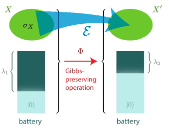
Figure 1: Implementation of a logical process $\mathcal{E}$ (any quantum process) using thermodynamic operations. The process acts on $X$ and has output on $X^{\prime}$, and is implemented by acting on the system and the battery with a joint Gibbs-preserving operation. The battery starts with a depletion state $\lambda_{1}$ and finishes with a depletion state $\lambda_{2}$. The overall extracted work is given by the difference $\lambda_{1}-\lambda_{2}$.

Given operators $\Gamma_{X},\Gamma_{X^{\prime}}\geqslant 0$, an input state $\sigma_{X}$, and a logical process $\mathcal{E}_{X\to X^{\prime}}$ (that is, a trace-nonincreasing, completely positive map), the task is to find the maximum number of qubits that can be extracted, or the minimum number of qubits that need to be invested, in order to implement the logical process on the given input state. Note that we require the correlations between the input and the output to match those specified by $\mathcal{E}_{X\to X^{\prime}}$, a condition that is not equivalent to just requiring that the given input state $\sigma_{X}$ is transformed into the given output state $\mathcal{E}_{X\to X^{\prime}}(\sigma_{X})$. Equivalently, we require that the implementation acts as the process $(\mathcal{E}_{X\to X^{\prime}}\otimes\operatorname{id}_{R_{X}})$ on a purified state $\lvert{\sigma}\rangle_{XR_{X}}$ of the input, where $\operatorname{id}_{R_{X}}$ denotes the identity process on $R_{X}$.

Finally, we ignore improbable events with total probability $\epsilon$, which is necessary in order to obtain meaningful physical results Alhambra et al. (2016b). Indeed, in textbook thermodynamics when calculating the work cost of compressing an ideal gas, for instance, one ignores the exceedingly unlikely event where all gas particles conspire to hit against the piston at much greater force than on average, a situation that would require more work for the compression but that happens with overwhelmingly negligible probability. For our purposes, we may optimize the zero-error work cost over states that are $\epsilon$-approximations of the required state Faist et al. (2015a), which is a standard approach in quantum information and cryptography Renner (2005); Tomamichel (2012).

At this point, it is useful to introduce the notion of the process matrix associated with the pair $(\mathcal{E}_{X\to X^{\prime}},\sigma_{X})$ of the logical process and input state. First, we define a reference system $R_{X}$ of the same dimension as $X$ and choose some fixed bases $\{\lvert{k}\rangle_{X}\}$ and $\{\lvert{k}\rangle_{R_{X}}\}$ of $X$ and $R_{X}$. Then, we define the process matrix of the pair $(\mathcal{E}_{X\to X^{\prime}},\sigma_{X})$ as the bipartite quantum state $\rho_{X^{\prime}R_{X}}=(\mathcal{E}_{X\to X^{\prime}}\otimes\operatorname{id}_{R_{X}})(\lvert{\sigma}\rangle\langle{\sigma}\rvert_{X:R_{X}})$, where $\lvert{\sigma}\rangle_{X:R_{X}}=\sigma_{X}^{1/2}\,(\sum\lvert{k}\rangle_{X}\otimes\lvert{k}\rangle_{R_{X}})$. The process matrix corresponds to the Choi matrix of $\mathcal{E}_{X\to X^{\prime}}$, yet it is “weighted” by the input state $\sigma_{X}$ in the sense that the reference state is $\sigma_{XR_{X}}$ instead of a maximally entangled state. The process matrix is in one-to-one correspondence with the pair $(\mathcal{E}_{X\to X^{\prime}},\sigma_{X})$ except for the part of $\mathcal{E}_{X\to X^{\prime}}$ that acts outside the support of $\sigma_{X}$; i.e., the specification of $\rho_{X^{\prime}R_{X}}$ uniquely determines $\sigma_{X}$ as well as the logical process $\mathcal{E}_{X\to X^{\prime}}$ on the support of $\sigma_{X}$. The reduced states $\sigma_{X}$ and $\sigma_{R_{X}}$ of $\lvert{\sigma}\rangle_{XR_{X}}$ are related by a partial transpose, $\sigma_{R_{X}}=\sigma_{X}^{T}$. Intuitively, the reference system $R_{X}$ may be thought of as a “mirror system” which “remembers” what the input state to the process was.

As a further remark, one might be worried that the relaxation of the set of allowed operations from $\Gamma$-preserving and trace-preserving maps to $\Gamma$-sub-preserving and trace-nonincreasing maps is too drastic. Indeed, while yielding a valid bound, the relaxed set of operations is unphysical and we might thus obtain a looser bound than necessary. In fact, this is not the case. Rather, trace-nonincreasing, $\Gamma$-sub-preserving processes are a technical convenience, which allows for more flexibility in the characterization of what the process effectively does in the situations of interest to us while ignoring other irrelevant situations; yet, ultimately, we show that an equivalent implementation can be carried out as a single trace-preserving, $\Gamma$-preserving map. For instance, consider a box separated into two equal-volume compartments, one of which contains a single-particle gas (a setup known as a Szilárd engine Szilard (1929)). The particle may be in one of two states, $\lvert{\mathrm{L}}\rangle,\lvert{\mathrm{R}}\rangle$, representing the particle being located in either the left or right compartment. If the particle is located in the left compartment, then work can be extracted by attaching a piston to the separator and letting the gas expand in contact with a heat bath. Yet, if we know the particle to be initially in the left compartment, it makes no difference what the process would have done had the particle been in the right compartment—that situation is irrelevant. Hence, we may define the corresponding “effective process” as the trace-nonincreasing map, which maps $\lvert{\mathrm{L}}\rangle$ to the maximally mixed state (allowing us to extract work) and which maps $\lvert{\mathrm{R}}\rangle$ to the zero vector. Evidently, the full actual physical implementation is a trace-preserving process, yet it is convenient to represent the “relevant part” of this process using a trace-nonincreasing map. Crucially, both mappings have the same process matrix, given that the input state is $\lvert{\mathrm{L}}\rangle$. This picture is justified on a formal level: We show that any trace-nonincreasing, $\Gamma$-sub-preserving map $\tilde{\Phi}$ can be dilated in the following way. There exists a trace-preserving, $\Gamma$-preserving map over an additional ancilla whose process matrix is as close to a given $\rho_{X^{\prime}R_{X}}$ as the process matrix of $\tilde{\Phi}$ combined with a transition on the ancilla between two eigenstates of the $\Gamma$ operator (Subsection D.1 in the Appendix).

III Results

III.1 Fundamental work cost of a process

Consider two systems $X$ and $X^{\prime}$ with corresponding operators $\Gamma_{X}$ and $\Gamma_{X^{\prime}}$, respectively, as described above and as imposed by the appropriate thermodynamic bath Barnett and Vaccaro (2013); Yunger Halpern and Renes (2016); Guryanova et al. (2016); Yunger Halpern et al. (2016). We consider any input state $\sigma_{X}$ as well as any logical process $\mathcal{E}_{X\to X^{\prime}}$, i.e., any completely positive, trace-preserving map. With a reference system $R_{X}$ of the same dimension as $X$, which purifies the input state as $\lvert{\sigma}\rangle_{XR_{X}}$, the logical process and the input state jointly define the process matrix $\rho_{X^{\prime}R_{X}}=(\mathcal{E}_{X\to{}X^{\prime}}\otimes\operatorname{id}_{R_{X}})(\sigma_{XR_{X}})$.

Our main result is phrased in terms of the coherent relative entropy, defined as

$$\hat{D}_{X\to X^{\prime}}^{\epsilon}(\rho_{X^{\prime}R_{X}}\|\Gamma_{X},\Gamma_{X^{\prime}})\leavevmode\nobreak\ =\leavevmode\nobreak\ \max_{\begin{subarray}{c}\mathcal{T}(\Gamma_{X})\leqslant 2^{-\lambda}\Gamma_{X^{\prime}}\\ \mathcal{T}(\sigma_{XR_{X}})\approx_{\epsilon}\rho_{X^{\prime}R_{X}}\end{subarray}}\lambda\ ,$$ (2)

where the optimization ranges over completely positive, trace-nonincreasing maps $\mathcal{T}_{X\to X^{\prime}}$. The notation ‘$\approx_{\epsilon}$’ signifies proximity of the quantum states in terms of the purified distance, a distance measure derived from the fidelity of the quantum states related to the ability to distinguish the two states by a measurement Tomamichel et al. (2010); Tomamichel (2012, 2016), which is closely related to the quantum angle, Bures distance and infidelity distance measures Bengtsson and Zyczkowski (2006); Nielsen and Chuang (2000).

The definition 2 is independent of which purification $\lvert{\sigma}\rangle_{XR_{X}}$ is chosen on $R_{X}$, noting that $\rho_{X^{\prime}R_{X}}$ also depends on this choice. Furthermore, we use the shorthand $\hat{D}_{X\to X^{\prime}}(\rho_{X^{\prime}R_{X}}\|\Gamma_{X},\Gamma_{X^{\prime}}):=\hat{D}_{X\to{}X^{\prime}}^{\epsilon=0}(\rho_{X^{\prime}R_{X}}\|\Gamma_{X},\Gamma_{X^{\prime}})$.

At this point, we may formulate our main contribution:

Main Result.

The optimal implementation of the process $\mathcal{E}_{X\to X^{\prime}}$ on the input state $\sigma_{X},$ with free operations acting jointly on the system $X$ and an information battery, can extract a number $\lambda_{\mathrm{optimal}}$ of pure qubits given by the coherent relative entropy,

$$\lambda_{\mathrm{optimal}}=\hat{D}_{X\to X^{\prime}}^{\epsilon}(\rho_{X^{\prime}R_{X}}\|\Gamma_{X},\Gamma_{X^{\prime}})\ .$$ (3)

If $\lambda_{\mathrm{optimal}}<0$, then the implementation needs to invest at least $-\lambda_{\mathrm{optimal}}$ pure qubits.

The resources required to carry out the process, counted in terms of $\lambda_{\mathrm{optimal}}$ pure qubits, may be converted into physical work. For instance, if we have access to a heat bath at temperature $T$, we may convert each pure qubit into $kT\ln(2)$ work and vice versa, and thus the work extracted by an optimal implementation of the process is

$$W=kT\ln(2)\cdot\hat{D}_{X\to X^{\prime}}^{\epsilon}(\rho_{X^{\prime}R_{X}}\|\Gamma_{X},\Gamma_{X^{\prime}})\ .$$ (4)

In fact, it is not necessary to implement the process using the information battery at all, and the resources may be directly supplied by a variety of other battery models. The work can even be supplied by a macroscopic pistonlike system, as we will see later.

Here, we provide the main technical ingredients to understand the idea of the proof of our main result, while deferring details to Appendix C and Appendix E.

A central step in our proof is a characterization of how much battery charge needs to be invested in order to implement exactly any completely positive, trace-nonincreasing map $\mathcal{T}_{X\to X^{\prime}}$. Such maps are those over which we optimize in 2 to define the coherent relative entropy. The work yield, or negative work cost, of performing $\mathcal{T}_{X\to X^{\prime}}$ with $\Gamma$-sub-preserving processes using an information battery is given by “how $\Gamma$-sub-preserving” the process is:

Proposition I.

Let $\mathcal{T}_{X\to X^{\prime}}$ be a completely positive, trace-nonincreasing map and let $y\in\mathbb{R}$. Then, the following are equivalent:

1. The map $\mathcal{T}_{X\to X^{\prime}}$ satisfies

   $$\mathcal{T}_{X\to X^{\prime}}(\Gamma_{X})\leqslant 2^{-y}\,\Gamma_{X^{\prime}}\ ;$$ (5)

2. For a large enough battery $A$ (with $\Gamma_{A}=\mathds{1}_{A}$) and for any $\lambda_{1},\lambda_{2}\geqslant 0$ such that $\lambda_{1}-\lambda_{2}\leqslant y$, there exists a trace-nonincreasing, $\Gamma$-sub-preserving map $\Phi_{XA\to X^{\prime}A}$ satisfying for all $\omega_{X}$,

   $$\Phi_{XA\to X^{\prime}A}\bigl{(}\omega_{X}\otimes\bigl{(}2^{-\lambda_{1}}\mathds{1}_{2^{\lambda_{1}}}\bigr{)}\bigr{)}\\ =\mathcal{T}_{X\to X^{\prime}}(\omega_{X})\otimes\bigl{(}2^{-\lambda_{2}}\mathds{1}_{2^{\lambda_{2}}}\bigr{)}\ ,$$ (6)

   where $2^{-\lambda}\mathds{1}_{2^{\lambda}}$ denotes a uniform mixed state of rank $2^{\lambda}$ on system $A$.

Proposition I shows that if there is an allowed operation in our framework which implements a given completely positive, trace-nonincreasing map $\mathcal{T}$ exactly while charging the battery by an amount $\lambda$, then the mapping must necessarily satisfy $\mathcal{T}(\Gamma)\leqslant 2^{-\lambda}\Gamma$. Conversely, for any trace-nonincreasing map $\mathcal{T}$ satisfying $\mathcal{T}(\Gamma)\leqslant 2^{-\lambda}\Gamma$ for some value $\lambda$, there exists an operation in our framework acting on the system and a battery system which implements $\mathcal{T}$ while charging the battery by some value $\lambda$. This operation is a trace-nonincreasing, $\Gamma$-sub-preserving map acting on the system and the battery. From this operation, we can then construct a fully $\Gamma$-preserving, trace-preserving map that implements $\mathcal{T}$, as argued at the end of the previous section.

Our main result then exploits Proposition I in order to answer the original question, that is, to find the optimal battery charge extraction when implementing approximately a logical process $\mathcal{E}$ on an input state $\sigma$. In effect, one needs to optimize the implementation cost over all maps $\mathcal{T}$ whose process matrix is $\epsilon$-close to the required process matrix. This optimization corresponds precisely to the one carried out in the definition of the coherent relative entropy in 2. (If $\sigma_{X}$ is full rank and if $\epsilon=0$, then necessarily $\mathcal{T}=\mathcal{E}$; in general, however, a better candidate $\mathcal{T}$ may be found.)

III.2 The coherent relative entropy and its properties

The coherent relative entropy $\hat{D}_{X\to X^{\prime}}^{\epsilon}(\rho_{X^{\prime}R_{X}}\|\Gamma_{X},\Gamma_{X^{\prime}})$ defined in 2 intuitively measures the amount of information discarded during the process, relative to the weights represented in $\Gamma_{X}$ and $\Gamma_{X^{\prime}}$. It ignores unlikely events of total probability $\epsilon$, a parameter that can be chosen freely. Its interpretation as a measure of information is justified by the collection of properties it satisfies, which are natural for such measures, and since it reproduces known results in special cases. We provide an overview of the properties of this quantity here, and refer to Appendix E for the technical details.

Elementary properties.

The coherent relative entropy obeys some trivial bounds. Specifically,

$$-\log_{2}\operatorname{tr}(\Gamma_{X})-\log_{2}\,\big{\lVert}{\Gamma_{X^{\prime}}^{-1}}\big{\rVert}_{\infty}$$

$$\hskip 30.00005pt\leqslant\leavevmode\nobreak\ \hat{D}_{X\to X^{\prime}}^{\epsilon}(\rho_{X^{\prime}R_{X}}\|\Gamma_{X},\Gamma_{X^{\prime}})+\log_{2}(1-\epsilon^{2})$$

$$\hskip 30.00005pt\leqslant\leavevmode\nobreak\ \log_{2}\,\big{\lVert}{\Gamma_{X}^{-1}}\big{\rVert}_{\infty}+\log_{2}\operatorname{tr}(\Gamma_{X^{\prime}})\ .$$ (7)

These bounds have a natural interpretation in the context of a single heat bath at inverse temperature $\beta=1/(kT)$. The extracted work may never exceed an amount corresponding to starting in the highest energy level of the system and finishing in the Gibbs state; similarly, it may never be less than the amount corresponding to starting in the Gibbs state and finishing in the highest excited energy level. (A correction is added to account for additional work that can be extracted by exploiting the $\epsilon$ accuracy tolerance.)

Under scaling of the $\Gamma$ operators, the coherent relative entropy simply acquires a constant shift: For any $a,b>0$,

$$\hat{D}_{X\to X^{\prime}}^{\epsilon}(\rho_{X^{\prime}R_{X}}\|a\Gamma_{X},b\Gamma_{X^{\prime}})\\ =\hat{D}_{X\to X^{\prime}}^{\epsilon}(\rho_{X^{\prime}R_{X}}\|\Gamma_{X},\Gamma_{X^{\prime}})+\log_{2}\frac{b}{a}\ .$$ (8)

In the case of a single heat bath at inverse temperature $\beta=1/(kT)$, this property simply corresponds to the fact that if the Hamiltonians of the input and output systems are translated by some constant energy shifts, then the difference in the shifts should simply be accounted for in the work cost. Indeed, if $H_{X}\to H_{X}+\Delta E_{X}$ and $H_{X^{\prime}}\to H_{X^{\prime}}+\Delta E_{X^{\prime}}$, then $\Gamma_{X}\to e^{-\beta\Delta E_{X}}\,\Gamma_{X}$, $\Gamma_{X^{\prime}}\to e^{-\beta\Delta E_{X^{\prime}}}\,\Gamma_{X^{\prime}}$ and the optimal extracted work of a process, given by $kT\ln(2)$ times the coherent relative entropy, has to be adjusted according to 8 by $kT\ln(2)\log_{2}(e^{-\beta\Delta E_{X^{\prime}}}/e^{-\beta\Delta E_{X}})=\Delta E_{X}-\Delta E_{X^{\prime}}$.

Recovering known entropy measures.

In special cases we recover known results in single-shot quantum thermodynamics, reproducing existing entropy measures from the smooth entropy framework Renner (2005); Tomamichel (2016).

In the case of a system described by a trivial Hamiltonian, the work cost of erasing a state to a pure state is given by the max-entropy Dahlsten et al. (2011), a measure that characterizes data compression or information reconciliation König et al. (2009); similarly, preparing a state from a pure state allows us to extract an amount of work given by the min-entropy of the state, a measure that characterizes the amount of uniform randomness that can be extracted from the state. These results turn out to be special cases of considering the work cost of any arbitrary quantum process for systems with a trivial Hamiltonian Faist et al. (2015a), which is given by the conditional max-entropy of the discarded information conditioned on the output of the process:

$$\hat{D}_{X\to X^{\prime}}^{\epsilon}(\rho_{X^{\prime}R_{X}}\|\mathds{1}_{X},\mathds{1}_{X^{\prime}})\\ \approx-\hat{H}_{\mathrm{max}}^{\epsilon}(E|X^{\prime})=\hat{H}_{\mathrm{min}}^{\epsilon}(E|R_{X})\ ,$$ (9)

where $\lvert{\rho}\rangle_{EX^{\prime}R_{X}}$ is a purification of $\rho_{X^{\prime}R_{X}}$ and where $\hat{H}_{\mathrm{max}}^{\epsilon}(E|X^{\prime})$ and $\hat{H}_{\mathrm{min}}^{\epsilon}(E|R_{X})$ are the smooth conditional max-entropy and min-entropy which were introduced in ref. Renner (2005), and are also known as the alternative conditional max-entropy and min-entropy Tomamichel et al. (2011). A precise meaning of the approximation in 9 is provided in Appendix E.

We recover more known results with an arbitrary Hamiltonian in contact with a heat bath by considering state formation and work extraction of a quantum state Åberg (2013); Horodecki and Oppenheim (2013). It is known that the work that can be extracted from a quantum state, or that is required to form a quantum state, is given by the min-relative entropy and the max-relative entropy, respectively; these single-shot relative entropies were introduced in ref. Datta (2009) and are related to hypothesis testing Buscemi and Datta (2010); Brandão and Datta (2011); Tomamichel and Hayashi (2013); Wang and Renner (2012); Matthews and Wehner (2014); Mosonyi2014CMP_hypothesis. We show that if the input or output system is trivial, then

$$\hat{D}_{X\to\varnothing}^{\epsilon}(\rho_{R_{X}}\|\Gamma_{X},1) \approx D_{\mathrm{min,0}}^{\epsilon}(\rho_{X}\|\Gamma_{X})\ ;$$ (10a)

$$\hat{D}_{\varnothing\to X^{\prime}}^{\epsilon}(\rho_{X^{\prime}}\|1,\Gamma_{X^{\prime}}) \approx-D_{\mathrm{max}}^{\epsilon}(\rho_{X^{\prime}}\|\Gamma_{X^{\prime}})\ ,$$ (10b)

matching the previously known results. We note that a trivial system as output or input of a process is equivalent to mapping to or from a pure, zero-energy eigenstate; this is because the coherent relative entropy is insensitive to energy eigenstates (or more generally, eigenstates of the $\Gamma$ operator) that have no overlap with the corresponding input or output state.

Data processing inequality and chain rule.

The coherent relative entropy satisfies a data processing inequality: If an additional channel is applied to the output, mapping the Gibbs weights to other Gibbs weights, then the coherent relative entropy may only increase. In other words, for any channel $\mathcal{F}_{X^{\prime}\to X^{\prime\prime}}$,

$$\hat{D}_{X\to X^{\prime}}^{\epsilon}(\rho_{X^{\prime}R_{X}}\|\Gamma_{X},\Gamma_{X^{\prime}})\\ \leqslant\hat{D}_{X\to X^{\prime\prime}}^{\epsilon}(\mathcal{F}_{X^{\prime}\to X^{\prime\prime}}(\rho_{X^{\prime}R_{X}})\|\Gamma_{X},\mathcal{F}_{X^{\prime}\to X^{\prime\prime}}(\Gamma_{X^{\prime}}))\ .$$ (11)

Intuitively, this holds because the final state after the application of $\mathcal{F}_{X^{\prime}\to X^{\prime\prime}}$ is less valuable as it is closer to the Gibbs state, and hence more work can be extracted by the optimal process realizing the total operation $X\to X^{\prime\prime}$.

The coherent relative entropy also obeys a natural chain rule: The work extracted during two consecutive processes may only be less than an optimal implementation of the total effective process. We refer to Appendix E for a technically precise formulation.

Asymptotic equipartition.

An important property of the coherent relative entropy is its asymptotic behavior in the limit of many independent copies of the process (known as the i.i.d. limit). In this regime, the coherent relative entropy converges to the difference in the quantum relative entropies of the input state to the output state, which is consistent with previous results in quantum thermodynamics Brandão et al. (2013, 2015):

$$\lim_{n\to\infty}\frac{1}{n}\hat{D}_{X^{n}\to X^{\prime n}}^{\epsilon}(\rho_{X^{\prime}R_{X}}^{\otimes n}\|\Gamma_{X}^{\otimes n},\Gamma_{X^{\prime}}^{\otimes n})\\ =D(\sigma_{X}\|\Gamma_{X})-D(\rho_{X^{\prime}}\|\Gamma_{X^{\prime}})\ ,$$ (12)

recalling that $\sigma_{X}$ is the input state of the process and $\rho_{X^{\prime}}$ the resulting output state, and where $\epsilon$ is small and either kept constant or taken to zero slower than exponentially in $n$. Crucially, the average work cost of performing a process in the i.i.d. regime with Gibbs-preserving operations does not depend on the details of the process, but only on the input and output states, as was already the case for systems described by a trivial Hamiltonian Faist et al. (2015a).

Miscellaneous properties.

We show a collection of further properties, including the following: The coherent relative entropy is equal to zero for a pure process matrix, which corresponds to an identity mapping, for any input state and for $\epsilon=0$; the smooth coherent relative entropy can be bounded in both directions as differences of known entropy measures; the coherent relative entropy does not depend on the details of the process if the input state is of the form $\Gamma_{X}/\operatorname{tr}(\Gamma_{X})$ (e.g., a Gibbs state), and it reduces, in this case, to a difference of input and output relative entropies and hence only depends on the output of the process.

III.3 Battery states and robustness to smoothing

Previous work has already shown the equivalence of several battery models known in the literature Brandão et al. (2015), notably the information battery, the work bit (“wit”) Horodecki and Oppenheim (2013); Brandão et al. (2015), and the “weight” system Skrzypczyk et al. (2014); Alhambra et al. (2016a). Our framework allows us to make this equivalence manifest, by singling out a class of states on any system for which the system can act as a battery. These states exhibit the property that they are reversibly interconvertible (as in ref. Gallego et al. (2016))—the resources invested in a transition from one battery state to another can be recovered entirely and deterministically by carrying out the reverse transition.

For any system $W$ with a corresponding $\Gamma_{W}$, we consider as battery states those states of the form

$$\tau(P)=\frac{P\Gamma_{W}P}{\operatorname{tr}(P\Gamma_{W})}\ ,$$ (13)

where $P$ is a projector such that $[P,\Gamma_{W}]=0$. In the presence of a single heat bath at inverse temperature $\beta$, this class of states includes, for instance, individual energy eigenstates or also maximally mixed states on a subspace of an energy eigenspace. We define the value of a particular battery state $\tau(P)$ as

$$\Lambda(\tau(P))=-\log_{2}\operatorname{tr}(P\Gamma_{W})\ .$$ (14)

We require the system $W$ to start in such a battery state $\tau(P)$ and to end in another such state $\tau(P^{\prime})$ corresponding to another projector $P^{\prime}$ with $[P^{\prime},\Gamma_{W}]=0$. The following proposition asserts that the system $W$ can act as a battery enabling exactly the same state transitions on another system $S$ as an information battery with charge difference $\lambda_{1}-\lambda_{2}=\Lambda(\tau(P^{\prime}))-\Lambda(\tau(P))$ (see Appendix C for proofs):

Proposition II.

Let $\mathcal{T}_{X\to X^{\prime}}$ be a completely positive, trace-nonincreasing map, and let $y\in\mathbb{R}$. Then, statements (a) and (b) in Proposition I are further equivalent to the following:

1. For any quantum system $W$ with corresponding $\Gamma_{W}$, and for any projectors $P,P^{\prime}$ satisfying $[P,\Gamma_{W}]=[P^{\prime},\Gamma_{W}]=0$ such that $\Lambda(\tau(P^{\prime}))-\Lambda(\tau(P))\leqslant y$, there exists a $\Gamma$-sub-preserving, trace-nonincreasing map $\Phi_{XW\to X^{\prime}W}$ such that for all $\omega_{X}$,

   $$\Phi_{XW\to X^{\prime}W}\bigl{(}\omega_{X}\otimes\tau(P)\bigr{)}=\mathcal{T}_{X\to X^{\prime}}(\omega_{X})\otimes\tau(P^{\prime})\ .$$ (15)

The information battery, the wit as well as the weight system are themselves special cases of this general battery system. Indeed, the states $2^{-\lambda_{i}}\mathds{1}_{2^{\lambda_{i}}}$ of the information battery can be cast in the form 13, with $P=\mathds{1}_{2^{\lambda_{i}}}$ since $\Gamma=\mathds{1}$ for the information battery; the corresponding value of the state is indeed $\Lambda(\tau(P))=-\lambda_{i}$. Similarly, in the case of the wit and of the weight system, and in the presence of a single heat bath at inverse temperature $\beta$ such that $\Gamma_{W}=e^{-\beta H_{W}}$, the relevant states are energy eigenstates $\lvert{E}\rangle_{W}$, whose value is precisely their energy, up to a factor $\beta$: $\Lambda(\tau(\lvert{E}\rangle\langle{E}\rvert_{W}))=\beta E$. The equivalence of these models is thereby manifest.

As can be expected, the battery states of the general form $\tau(P)$ are reversibly interconvertible, implying that for any process that maps $\tau(P)$ to $\tau(P^{\prime})$ on a system, the coherent relative entropy is equal to the difference $\Lambda(\tau(P))-\Lambda(\tau(P^{\prime}))$.

This general formulation enables us to prove an interesting property of these battery states—they are robust to small imperfections. Indeed, when implementing a process on a system $S$ using a battery $W$, it makes no difference whether one optimizes over $\epsilon$-approximations of the overall process on the joint system $S\otimes W$, or over $\epsilon$-approximations on $S$ only with no imperfections on the battery state (as the smooth coherent relative entropy is defined above). More precisely, we prove that the smooth coherent relative entropy is exactly the optimal difference in the charge state of the battery while capturing all implementations that include slight imperfections on the battery for any battery system:

$$\hat{D}_{X\to X^{\prime}}^{\epsilon}(\rho_{X^{\prime}R_{X}}\|\Gamma_{X},\Gamma_{X^{\prime}})\\ =\max_{\begin{subarray}{c}W,P_{W},P^{\prime}_{W},\\ \Phi_{XW\to X^{\prime}W}\end{subarray}}-\log_{2}\frac{\operatorname{tr}(P^{\prime}_{W}\Gamma_{W})}{\operatorname{tr}(P_{W}\Gamma_{W})}\ ,$$ (16)

where the optimization ranges over all battery systems $W$ with corresponding $\Gamma_{W}$, over all battery states corresponding to projectors $P_{W},P^{\prime}_{W}$ with $[P_{W},\Gamma_{W}]=[P^{\prime}_{W},\Gamma_{W}]=0$, and over all free operations $\Phi_{XW\to X^{\prime}W}$ which are an $\epsilon$-approximation of a joint process $XW\to X^{\prime}W$, with a resulting process matrix on the system of interest given by $\rho_{X^{\prime}R_{X}}$ and which induces a transition on the battery from $\tau(P_{W})$ to $\tau(P^{\prime}_{W})$ (see Appendix G).

III.4 Emergence of macroscopic thermodynamics

We now apply our general framework to the case of macroscopic systems, and recover the standard laws of thermodynamics as emergent from our model. On one hand, the goal of this section is to show that our framework behaves as expected in the macroscopic limit, further justifying it as a model for thermodynamics. On the other hand, the arguments presented here reinforce the picture of the macroscopic laws of thermodynamics as emergent from microscopic dynamics, in line with common knowledge and existing literature Lieb and Yngvason (1999, 2004); Brandão et al. (2013, 2015); Tajima et al. (2016); Chubb et al. (2017a), by providing an alternative explanation of this emergence based on $\Gamma$-sub-preserving maps. (In fact, this emergence may be understood as defining the order relation in refs. Lieb and Yngvason (1999, 2004, 2013, 2014); Weilenmann et al. (2016) as the ordering induced by transformation by $\Gamma$-sub-preserving maps).

The general mechanism.

The macroscopic theory of thermodynamics is recovered when it is possible to single out a class of states that obey a reversible interconversion property. More precisely, suppose there are a class of states $\{\tau^{z_{1},z_{2},\ldots,z_{m}}\}$ specified by $m$ parameters $z_{1},\ldots,z_{m}$, and suppose there exists a potential $\Lambda(z_{1},\ldots,z_{m})$ such that for any pair of states $\tau_{X}^{z_{1},\ldots,z_{m}}$ and $\tau_{X^{\prime}}^{z^{\prime}_{1},\ldots,z^{\prime}_{m}}$ from this class, we have, for any process matrix $\rho_{X^{\prime}R_{X}}$ mapping one state to the other,

$$\ln(2)\cdot\hat{D}_{X\to X^{\prime}}(\rho_{X^{\prime}R_{X}}\|\Gamma_{X},\Gamma_{X^{\prime}})\\ =\Lambda(z_{1},\ldots,z_{m})-\Lambda(z^{\prime}_{1},\ldots,z^{\prime}_{m})\ .$$ (17)

The $\ln(2)$ factor merely serves to change the units of the coherent relative entropy from bits, which is standard in information theory, to nats, which will prove convenient to recover the standard laws of thermodynamics. We call the function $\Lambda(z_{1},\ldots,z_{m})$ the natural thermodynamic potential corresponding to the physics encoded in the $\Gamma$ operators. In other words, the two states $\tau^{z_{1},\ldots,z_{m}}$ and $\tau^{z^{\prime}_{1},\ldots,z^{\prime}_{m}}$ may be reversibly interconverted, as any work invested when going in one direction may be recovered when returning to the initial state, and this is irrespective of which precise logical process is effectively carried out during the transition. An obvious choice of states with this property are states of the same form as the battery states introduced above, which motivates recycling the same symbols $\tau$ and $\Lambda$. (We have set $\epsilon=0$ in 17 because smoothing such battery-type states has no significant effect.)

Suppose that the parameters are sufficiently well approximated by continuous values. This would typically be the case for a large system such as a macroscopic gas. Consider an infinitesimal change of a state $(z_{1},\ldots,z_{m})\to(z_{1}+dz_{1},\ldots,z_{m}+dz_{m})$. If there is a free operation that can perform this transition, then necessarily, the coherent relative entropy is positive; hence, $\Lambda(z_{1}+dz_{1},\ldots,z_{m}+dz_{m})\leqslant\Lambda(z_{1},\ldots,z_{m})$. Conversely, if the coherent relative entropy is positive, then there necessarily exists a free operation implementing the said transition. We deduce that the infinitesimal transition $z\to z+dz$ is possible with a free operation if and only if

$$d\Lambda\leqslant 0\ .$$ (18)

This condition expresses the macroscopic second law of thermodynamics, as we will see below.

We may define the generalized chemical potentials

$$\mu_{i}=\left(\frac{\partial\Lambda}{\partial z_{i}}\right)_{z_{1},\ldots,z_{i-1},z_{i+1},\ldots,z_{m}}\ ,$$ (19)

where the notation $(\partial f/\partial x)_{y,z}$ denotes the partial derivative with respect to $x$ of a function $f$, as $y$ and $z$ are kept constant. We may then write the differential of $\Lambda$ as

$$d\Lambda=\sum\mu_{i}\,dz_{i}\ .$$ (20)

The generalized potentials $\mu_{i}$ are often directly related to physical properties of the system in question, such as temperature, pressure, or chemical potential.

Under external constraints on the variables $z_{1},z_{2},\ldots,z_{m}$, we may ask what the “most useless thermodynamic state” compatible with those conditions is. The answer is given by minimizing the potential $\Lambda$ subject to those constraints—this is a variational principle. For instance, if two systems with natural thermodynamic potentials $\Lambda_{1}(z_{1},\ldots,z_{m})$ and $\Lambda_{2}(z_{1}^{\prime},\ldots,z_{m}^{\prime})$ are put into contact under the constraints that for all $i$, $z_{i}+z_{i}^{\prime}$ must be kept constant (such as for extensive variables in thermodynamics), then we may write $dz_{i}=-dz_{i}^{\prime}$ and minimize $\Lambda=\Lambda_{1}+\Lambda_{2}$ by requiring that

$$0=d\Lambda=\sum(\mu_{i}-\mu_{i}^{\prime})\,dz_{i}\ ,$$ (21)

and we see that the minimum is attained when $\mu_{i}=\mu_{i}^{\prime}$. If the system is undergoing suitable thermalizing dynamics, then its evolution will naturally converge towards that point.

The textbook thermodynamic gas.

We proceed to recover the usual laws of thermodynamics in this fashion for a macroscopic isolated gas $S$ composed of many particles (Fig. 2).

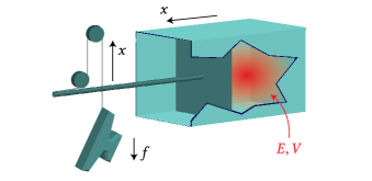
Figure 2: Macroscopic thermodynamics emerges from our framework when singling out a set of states that can be parametrized by continuous parameters to a good approximation and can be reversibly interconverted into one another. We consider the case of a textbook thermodynamic gas confined in a box, with a piston capable of furnishing work. In this setting, we recover the usual second law of thermodynamics, $dS\geqslant\delta Q/T$, relating the change in entropy, the dissipated heat, and the temperature.

The Hamiltonian of the gas is denoted by $H^{(V)}$, where the volume $V$ occupied by the gas is a classical parameter of the Hamiltonian that determines, for instance, the width of a confining potential. We assume, for simplicity, that the number $N$ of particles constituting the gas is kept at a fixed value throughout, restricting our considerations to the corresponding subspace.

Let us first consider the case of an isolated gas at fixed parameters $E,V$. In order to apply our framework, we must identify the $\Gamma$ operator, which encodes the relevant restrictions imposed by the physics of our system. Recall that our restriction is meant to explicitly forbid certain types of processes, without worrying whether a nonforbidden operation is achievable. Here, we assume that at fixed $E,V$, the system is isolated and hence evolves unitarily. In particular, the projector $P^{E,V}_{S}$ onto the eigenspace of $H^{(V)}$ corresponding to energy $E$ is preserved. Hence, the $\Gamma$ operator characterizing the gas alone for fixed $E,V$ can be taken as

$$\Gamma_{S}^{E,V}=P^{E,V}_{S}\ .$$ (22)

This is compatible with standard considerations in statistical mechanics, which identify the state of the gas in such conditions as the maximally mixed state in the subspace projected onto by $P^{E,V}_{S}$ (the microcanonical state), which we denote by $\tau_{S}^{E,V}=P^{E,V}_{S}/\operatorname{tr}(P^{E,V}_{S})$. Indeed, at fixed $E,V$ on the control system, an allowed transformation may not change this state.

Now, we would like to account for changes in $E,V$. It is convenient to introduce a physical control system $C$, which plays the following roles: It stores the information about all the controlled external parameters of the state in which the gas was prepared—here, the parameters are $E,V$; furthermore, it provides the necessary physical constraints on the gas and physical resources necessary for transformations, taking on the role of a battery. In our case, the control system includes a piston that confines the gas to a volume $V$ and is capable of furnishing the energy required to change the state of the gas. For concreteness, we imagine that the piston is balanced by a weight, causing the piston to exert a force $f$ on the gas. The force $f$ may be tuned by varying the weight. The states of the control system are $\lvert{e,x}\rangle_{C}$, where $e$ is the energy stored in the control system and $x$ the position of the piston. The energy $e$ is the potential energy of the weight, and it must be equal to $e=E_{\mathrm{tot}}-E$ as enforced by total energy conservation, where $E_{\mathrm{tot}}$ is the fixed total energy of the joint $CS$ system. Furthermore, $x$ determines the volume of the gas as $V=A\cdot x$, where $A$ is the surface of the piston. If the control system were isolated and not coupled to the gas, then the nonforbidden operations on the control system would be those preserving the operator $\Gamma_{C}^{0}=\sum_{e,x}g_{e,x}\lvert{e,x}\rangle\langle{e,x}\rvert_{C}$, where $g_{e,x}$ encodes the relevant physics of the control system: It decreases as either $e$ increases or $x$ increases, meaning that a state $\lvert{e,x}\rangle_{C}$ cannot be brought to the state $\lvert{e^{\prime},x}\rangle_{C}$ with $e^{\prime}>e$ or $\lvert{e,x^{\prime}}\rangle_{C}$ with $x^{\prime}>x$. In other words, we do not forbid reducing the weight charge or lowering it.

The coupling between the control system and the gas can be enforced with a $\Gamma$ operator of the form

$$\Gamma_{CS}=\sum_{e,x}g_{e,x}\lvert{e,x}\rangle\langle{e,x}\rvert_{C}\otimes P^{E=E_{\mathrm{tot}}-e,V=Ax}_{S}\ .$$ (23)

If the control system is the state $\lvert{e,x}\rangle_{C}$, then any allowed operation must preserve the operator $\Gamma^{E,V}_{S}$ for the corresponding $E=E_{\mathrm{tot}}-e$ and $V=Ax$. Furthermore 23 accounts for the physics of the control system itself with the coefficient $g_{e,x}$.

The states $\tau_{CS}^{e,x}=\lvert{e,x}\rangle\langle{e,x}\rvert_{C}\otimes\tau_{S}^{E=E_{\mathrm{tot}}-e,V=Ax}$ are of the form 13; hence, they are reversibly interconvertable as per 17 and they are a valid class of states for our macroscopic description. The corresponding natural thermodynamic potential is given as per 14,

$$\Lambda_{CS}(e,x) =\Lambda_{C}(e,x)+\Lambda_{S}(E_{\mathrm{tot}}-e,Ax)\ ,$$ (24)

where we have defined $\Lambda_{C}(e,x)=-\ln g_{e,x}$ and $\Lambda_{S}(E,V)=-\ln\operatorname{tr}(P^{E,V}_{S})$. Observe that $\operatorname{tr}P^{E,V}_{S}=\Omega_{S}(E,V)$ is the microcanonical partition function, and hence $\Lambda_{S}(E,V)$ is, up to Boltzmann’s constant $k$ and a minus sign, the quantity $S(E,V)=k\ln\Omega_{S}(E,V)$, which is known as the thermodynamic entropy of the gas:

$$\Lambda_{S}(E,V)=-k^{-1}S(E,V)\ .$$ (25)

As the gas is macroscopic, we assume that the parameters $E,V$ are well approximated by continuous variables. It is useful to define the conjugate variables to $e,x$ and $E,V$ via the differentials of $\Lambda_{C}$ and $\Lambda_{S}$:

$$d\Lambda_{C} =\nu_{e}\,de+\nu_{x}\,dx\ ;$$ (26a)

$$d\Lambda_{S} =\mu_{E}\,dE+\mu_{V}\,dV\ ,$$ (26b)

with the coupling inducing the relations $dE=-de$ and $dV=A\,dx$. The force $f$ exerted by the piston onto the gas is given by $f=(\partial e/\partial x)_{\Lambda_{C}}$. Using 26a we see that $de=\nu_{e}^{-1}(d\Lambda_{C}-\nu_{x}dx)$, and hence $f=-\nu_{x}/\nu_{e}$. The thermodynamic work provided by the piston is the mechanical work performed by the weight,

$$\delta W=-f\cdot dx=\frac{\nu_{x}}{\nu_{e}}\,dx\ .$$ (27)

Any operation mapping two states $\tau_{CS}^{e,x}\to\tau_{CS}^{e+de,x+dx}$ which obeys our global restriction, i.e. which preserves the operator 23, must obey 18 or, equivalently, $d\Lambda_{S}\leqslant-d\Lambda_{C}$; hence,

$$d\Lambda_{S}\leqslant-\nu_{e}\,de-\nu_{x}\,dx=\nu_{e}\,(dE-\delta W)=\nu_{e}\,\delta Q\ ,$$ (28)

where we have defined the change in energy of the gas that is not due to thermodynamic work as heat: $\delta Q=dE-\delta W$.

The temperature of the gas is defined as $T_{\mathrm{gas}}=(\partial S/\partial E)^{-1}=-(k\mu_{E})^{-1}$ as in standard textbooks, as the conjugate variable corresponding to entropy. The control system also acts as a heat bath, so we define its temperature $T$ as the temperature of a gas that it would be “in equilibrium” with, in the sense that our variational principle is achieved. The potential $\Lambda_{CS}$ attains its minimum under the constraints $dE=-de$ and $dV=A\cdot dx$ if $0=d\Lambda_{CS}=(\mu_{E}-\nu_{e})\,dE+(\mu_{V}+A^{-1}\nu_{x})\,dV$, implying that $\mu_{E}=\nu_{e}$ and hence $T=-(k\nu_{e})^{-1}$. We may now write 28 in its more traditional form,

$$dS\geqslant\frac{\delta Q}{T}\ .$$ (29)

Our control system is in fact another example of a battery system. Indeed, it can convert another form of a useful resource, mechanical work, into the equivalent of pure qubits for enabling processes on the system, while still working under the relevant global constraints such as conservation of energy.

The thermodynamic gas illustrates a situation in which the macroscopic second law of thermodynamics is recovered as emergent. Note that the argument can also be applied to a system with different relevant physical quantities, such as magnetic field and magnetization of a medium.

III.5 Observers in thermodynamics

In standard thermodynamics, one describes systems from the macroscopic point of view. This point of view is usually assumed only implicitly, to the point that notions such as thermal equilibrium or the thermodynamic entropy function are often thought of as objective properties of the system. Yet, a closer look reveals that they can be thought of as observer-dependent quantities, which can be extended to observers with different amounts of knowledge about the system Jaynes (1992); del Rio et al. (2011, 2016). This observation is at the core of a modern understanding of Maxwell’s demon.

The present section begins with a brief motivation, reviewing a variant of Maxwell’s demon. Then, we show that our framework is well suited for describing different observers and that it provides a natural notion of coarse-graining. Indeed, the framework itself, thanks to the abstraction provided by the $\Gamma$ operator, is scale agnostic and can be applied consistently from any level of knowledge about the system. More precisely, we show how to relate two descriptions from the viewpoints of two observers, where one observer sees a coarse-grained version of another observer’s knowledge. The coarse-graining is given by any completely positive, trace-preserving map. We define a sense in which we can carry out the reverse transformation, where one recovers the fine-grained information, given the coarse-grained information, with the help of a recovery map. This allows us to relate the laws of thermodynamics in either observer’s picture, where by the “laws of thermodynamics” in an observer’s picture, we mean that the evolution of the system is governed in their picture by $\Gamma$-sub-preserving maps. This provides a precise criterion that can guarantee, in a given setting, that the laws of thermodynamics hold in the coarse-grained picture or, intuitively, that “no Maxwell-demon-type cheating” is happening. Namely, if the fine-grained picture has no more information than what can be recovered from the coarse-grained picture, then our framework may be applied consistently from either picture, with both observers agreeing on the class of possible processes.

Consider the variant of Maxwell’s demon depicted in Fig. 3.

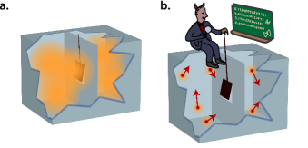
Figure 3: Maxwell’s demon concentrates all particles on one side of the box by opening the trap door at appropriate times. a. A macroscopic observer describing only the gas sees its entropy decrease, in apparent violation of the macroscopic observer’s idea of the second law of thermodynamics. b. The demon observes no entropy change, as the state of the gas is conditioned on his knowledge. By modeling his memory as an explicit system, originally in a pure state, we may understand his actions as simply correlating his memory with the state of the gas. In doing so, a macroscopic observer may be induced into witnessing a violation of a macroscopic second law. If the demon wishes to operate cyclically, he needs to reset his memory register back to a pure state, which costs work according to Landauer’s principle Bennett (1982, 2003); any work he might have extracted using his scheme is paid back at this point.

A gas is enclosed in a box separated into two equal volume compartments, which communicate only through a small trap door controlled by a demon. The demon is able to observe individual particles and activates the trap door at appropriate times, letting a single particle through each time, in order to concentrate all particles on one side of the box. From a macroscopic perspective, and looking only at the gas, one observes an apparent entropy decrease as the gas now occupies a smaller volume. However, from a microscopic perspective, the demon is essentially transferring entropy from the gas into a memory register, which is initially in a pure state Bennett (1982, 2003). Consider in more detail the following process: The demon performs a series of cnot gates using the gas degrees of freedom as controls and his memory qubits as targets, which “replicates” the information about the gas particles into his memory. Since this process is unitary, it preserves the joint entropy of the memory and the gas. The result is a classically correlated state between the memory register and the gas. So, what is the entropy of the gas? It is now clear that the answer depends on the observer. The macroscopic observer sees the gas with its usual macroscopic thermodynamic entropy, while the demon has engineered a state where the gas has zero entropy conditioned on the side information stored in his memory—he knows all there is to know about the gas. Conceptually, the thermodynamic reason for this difference is that the demon is able to extract work from the gas, whereas the macroscopic observer is not. Indeed, the demon can exploit the side information stored in his memory to design a perfect trap-door opening schedule which, when executed, concentrates all the particles on one side of the box. (This process can itself be thought of as cnot gates acting in the other direction.) With all particles concentrated on one side of the box, the demon can now extract work by replacing the separator by a piston and letting the gas expand isothermally. (Of course, the memory register is still littered with all the information about the gas; resetting the register costs work according to Landauer’s principle, which is where the demon pays back his extracted work if he wishes to operate cyclically Bennett (1982, 2003).)

The above example shows that a fully general framework of thermodynamics should be universally applicable from the point of view of any observer, accounting for any level of knowledge one might possess about a system. One also expects that if an observer sees a violation of their laws of thermodynamics, while knowing that in a finer-grained picture the corresponding laws are obeyed, then they may attribute this effect to lack of knowledge about microscopic degrees of freedom which the observed process exploits. In the following, we show that our framework displays these desired properties.

Consider two observers, Alice and Bob, who have distinct degrees of knowledge about a system. We assume that the system’s microscopic state space $\mathscr{H}_{A}$, which Alice has access to, is transformed by a completely positive, trace-preserving map $\mathcal{F}^{\mathcal{A}\to\mathcal{B}}_{A\to B}$ to a state space $\mathscr{H}_{B}$ which is used by Bob to describe the situation (Fig. 4).

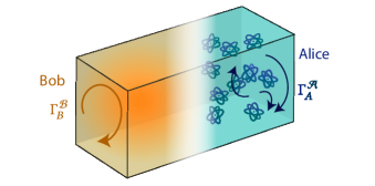
Figure 4: Observers in thermodynamics. Alice has access to microscopic degrees of freedom of a gas, while Bob can only observe its coarse macroscopic properties, such as its temperature $T$, volume $V$ and pressure $p$. Alice describes the evolution of the gas using Gibbs-preserving maps, with a Gibbs state $\Gamma_{A}^{\mathcal{A}}$ on the full state space of the many particles of the gas. On the other hand, Bob describes the gas using his own knowledge—for instance, the macroscopic variables $T,V,p$—which in full generality we can represent as a quantum state in a state space $\mathscr{H}_{B}$ which is obtained by applying a given mapping $\mathcal{F}_{A\to B}^{\mathcal{A}\to\mathcal{B}}(\cdot)$ on Alice’s state. (For instance, this map may trace out the inaccessible microscopic information.) States of the gas described by Bob may be transformed to Alice’s picture by applying a suitable recovery map, such as the Petz map Petz (1986, 1988, 2003); Wilde (2015); Beigi et al. (2016); Alhambra et al. (2015). Then, Alice’s $\Gamma_{A}^{\mathcal{A}}$-preserving maps appear to Bob as $\Gamma_{B}^{\mathcal{B}}$-preserving maps, where Bob’s $\Gamma_{B}^{\mathcal{B}}$ operator is taken to be $\Gamma_{B}^{\mathcal{B}}=\mathcal{F}_{A\to{}B}^{\mathcal{A}\to\mathcal{B}}(\Gamma_{A}^{\mathcal{A}})$. Conversely, operations that preserve $\Gamma_{B}^{\mathcal{B}}$ for Bob may be described by Alice as preserving $\Gamma_{A}^{\mathcal{A}}$.

For instance, Alice might have access to individual position and momenta of all the particles of a gas, while Bob only has access to partial information given by macroscopic physical quantities such as temperature, pressure, volume, etc. More generally, if the microscopic system can be embedded in a bipartite system $\mathscr{H}_{K}\otimes\mathscr{H}_{N}$ that stores, respectively, the macroscopic information (available to both Bob and Alice) and the microscopic information (available to Alice only), then Bob’s observations can be related to Alice’s simply by tracing out the $\mathscr{H}_{N}$ system.

Suppose that Alice observes some microscopic dynamics happening within $\mathscr{H}_{A}$ and that this evolution is $\Gamma$-preserving with a particular operator $\Gamma_{A}^{\mathcal{A}}$. How does this evolution appear to Bob? It turns out that for Bob, these maps are also $\Gamma$-preserving maps, but they are relative to his $\Gamma$ operator, which is simply given as $\Gamma_{B}^{\mathcal{B}}=\mathcal{F}^{\mathcal{A}\to\mathcal{B}}_{A\to{}B}(\Gamma_{A}^{\mathcal{A}})$, that is, by transforming Alice’s $\Gamma$ operator into Bob’s picture. Conversely, a map that appears as $\Gamma^{\mathcal{B}}$-preserving to Bob is observed by Alice as being $\Gamma^{\mathcal{A}}$-preserving.

In order to give a precise meaning to the above statements, it is necessary to specify how a state described by Bob can be translated back to Alice’s picture. Indeed, there can be several possible states for Alice that are compatible with Bob’s state. We describe this “recovery process” using a recovery map, which gives, in a sense, the “best guess” of what the state on $\mathscr{H}_{A}$ could be, given only knowledge of Bob’s state on $\mathscr{H}_{B}$. More precisely, we define the state transformation from Bob’s picture to Alice’s picture as the application of a completely positive, trace-preserving map $\mathcal{R}_{B\to A}^{\mathcal{B}\to\mathcal{A}}(\cdot)$, with the property that $\mathcal{R}_{B\to A}^{\mathcal{B}\to\mathcal{A}}(\Gamma_{B}^{\mathcal{B}})=\Gamma_{A}^{\mathcal{A}}$, recalling that $\Gamma^{\mathcal{B}}_{B}=\mathcal{F}^{\mathcal{A}\to\mathcal{B}}_{A\to B}(\Gamma^{\mathcal{A}}_{A})$. This ensures that the completely useless state in Bob’s picture is mapped back to the completely useless state in Alice’s picture. An example of a suitable recovery map is the Petz recovery map Petz (1986, 1988, 2003); Wilde (2015); Beigi et al. (2016); Alhambra et al. (2015), defined as

$$\mathcal{R}_{B\to A}^{\mathcal{B}\to\mathcal{A}}(\cdot)=\Gamma^{\mathcal{A}\,1/2}_{A}\,\mathcal{F}^{\mathcal{A}\leftarrow\mathcal{B}\,\dagger}_{A\leftarrow B}\bigl{(}\Gamma^{\mathcal{B}\,-1/2}_{B}\,(\cdot)\,\Gamma^{\mathcal{B}\,-1/2}_{B}\bigr{)}\,\Gamma^{\mathcal{A}\,1/2}_{A}\ ,$$ (30)

where $\mathcal{F}^{\mathcal{A}\leftarrow\mathcal{B}\,\dagger}_{A\leftarrow B}$ is the adjoint of the superoperator $\mathcal{F}^{\mathcal{A}\to\mathcal{B}}_{A\to B}$. The Petz recovery map is completely positive and trace preserving, and satisfies $\mathcal{R}_{B\to A}^{\mathcal{B}\to\mathcal{A}}(\Gamma_{B}^{\mathcal{B}})=\Gamma_{A}^{\mathcal{A}}$ (assuming that $\Gamma_{B}^{\mathcal{B}}$ is full rank).

Hence, given a trace-nonincreasing mapping $\mathcal{E}^{\mathcal{A}}_{A}$ in Alice’s picture, we define Bob’s description of the mapping as the composed map of transforming into Alice’s picture, applying the map, and transforming back to Bob’s picture:

$$\mathcal{E}^{\mathcal{B}}_{B}=\mathcal{F}^{\mathcal{A}\to\mathcal{B}}_{A\to B}\circ\mathcal{E}^{\mathcal{A}}_{A}\circ\mathcal{R}_{B\to{A}}^{\mathcal{B}\to\mathcal{A}}\ .$$ (31)

Our claim is the following: If $\mathcal{E}^{\mathcal{A}}_{A}$ satisfies $\mathcal{E}^{\mathcal{A}}_{A}(\Gamma^{\mathcal{A}}_{A})\leqslant\Gamma^{\mathcal{A}}_{A}$, then $\mathcal{E}^{\mathcal{B}}_{B}$ satisfies $\mathcal{E}^{\mathcal{B}}_{B}(\Gamma^{\mathcal{B}}_{B})\leqslant\Gamma^{\mathcal{B}}_{B}$. Conversely, if we are given a trace-nonincreasing mapping $\mathcal{E}^{\mathcal{B}}_{B}$ in Bob’s picture, then this map is described in Alice’s picture as the composed map of transforming to Bob’s picture, applying the map, and transforming back:

$$\mathcal{E}^{\mathcal{A}}_{A}=\mathcal{R}_{B\to{A}}^{\mathcal{B}\to\mathcal{A}}\circ\mathcal{E}^{\mathcal{B}}_{B}\circ\mathcal{F}^{\mathcal{A}\to\mathcal{B}}_{A\to{}B}\ ;$$ (32)

we assert that if $\mathcal{E}^{\mathcal{B}}_{B}(\Gamma^{\mathcal{B}}_{B})\leqslant\Gamma^{\mathcal{B}}_{B}$, then $\mathcal{E}^{\mathcal{A}}_{A}(\Gamma^{\mathcal{A}}_{A})\leqslant\Gamma^{\mathcal{A}}_{A}$.

The proof of both claims is straightforward, using $\mathcal{F}_{A\to{B}}^{\mathcal{A}\to\mathcal{B}}(\Gamma_{A}^{\mathcal{A}})=\Gamma_{B}^{\mathcal{B}}$ and $\mathcal{R}_{B\to{A}}^{\mathcal{B}\to\mathcal{A}}(\Gamma^{\mathcal{B}}_{B})=\Gamma^{\mathcal{A}}_{A}$. More generally, these claims hold as well for any trace-nonincreasing, completely positive maps $\mathcal{F}_{A\to{}B}^{\mathcal{A}\to\mathcal{B}}$, $\mathcal{R}_{B\to{}A}^{\mathcal{B}\to\mathcal{A}}$ satisfying $\mathcal{F}_{A\to{}B}^{\mathcal{A}\to\mathcal{B}}(\Gamma_{A}^{\mathcal{A}})\leqslant\Gamma_{B}^{\mathcal{B}}$ and $\mathcal{R}_{B\to{}A}^{\mathcal{B}\to\mathcal{A}}(\Gamma_{B}^{\mathcal{B}})\leqslant\Gamma_{A}^{\mathcal{A}}$, in which case $\Gamma_{B}^{\mathcal{B}}$ does not have to be full rank.

The above provides a general criterion that is able to guarantee that the laws of thermodynamics in the coarse-grained picture are valid: If the state of the system in Alice’s picture is one that can be recovered from Bob using a fixed recovery map, then Alice’s free operations correspond to free operations in Bob’s picture, and hence Alice’s laws of thermodynamics indeed translate to Bob’s idea of what the laws of thermodynamics are.

A simple example is the relation of the microcanonical to the canonical ensemble. (This is also known as Gibbs-rescaling, an essential tool to relate thermal operations to noisy operations Egloff et al. (2015); Horodecki and Oppenheim (2013); Brandão et al. (2015).) If Alice describes unitary dynamics within an energy eigenspace of the joint system and a large heat bath, then Bob describes the dynamics of the system alone as Gibbs-preserving maps. Consider a system $S$ and a heat bath $R$, with respective Hamiltonians $H_{S}$ and $H_{R}$ and total Hamiltonian $H_{SR}=H_{S}+H_{R}$. Suppose that Alice has microscopic access to the heat bath and hence describes the situation using the state space $A=S\otimes R$. Assume that the global state and evolution are constrained to unitaries within a subspace of fixed total energy $E$. This evolution is, in particular, $\Gamma$-sub-preserving if we choose $\Gamma^{\mathcal{A}}_{A}=P_{SR}^{E}$, where $P_{SR}^{E}$ is the projector onto the eigenspace of $H_{SR}$ corresponding to the energy $E$. On the other hand, Bob only has access to the system $B=S$. The mapping $\mathcal{F}^{\mathcal{A}\to\mathcal{B}}$, which relates Alice’s point of view to Bob’s, simply traces out the heat bath $R$. Bob then describes the operator $\Gamma^{\mathcal{A}}_{A}$ as

$$\Gamma^{\mathcal{B}}_{S}=\operatorname{tr}_{R}(\Gamma^{\mathcal{A}}_{SR})=\sum_{E_{S},k}g(E-E_{S})\,\lvert{E_{S},k}\rangle\langle{E_{S},k}\rvert_{S}\ ,$$ (33)

where $g(E_{R})$ is the degeneracy of the energy eigenspace of the heat bath corresponding to the energy $E_{R}$, and where the vectors $\{\lvert{E_{S},k}\rangle_{S}\}$ are the energy eigenstates on $S$ with a possible degeneracy index $k$. Following standard arguments in statistical mechanics, and as argued in ref. Horodecki and Oppenheim (2013), we have, in typical situations and under mild assumptions, $g(E-E_{S})\propto e^{-\beta E_{S}}$, and we hence recover in 33 the standard canonical form of the thermal state. In other words, Bob describes the dynamics on $S$ as maps that preserve the Gibbs state.

The above reasoning can be seen as a rule for transforming one observer’s picture into another; it remains important to analyze the situation in the picture that accurately describes the state of knowledge of the input state of the agent carrying out the operations. The pictures are equivalent when Alice’s state of knowledge of $A$ is no more than what $B$ can recover using the recovery map, i.e., when her input state is exactly of the form $\mathcal{R}_{B\to A}^{\mathcal{B}\to\mathcal{A}}(\rho_{B}^{\mathcal{B}})$, where $\rho_{B}^{\mathcal{B}}$ is the state of the system in Bob’s picture. However, not all actions that Alice can perform using $\Gamma^{\mathcal{A}}_{A}$-sub-preserving maps must induce a $\Gamma^{\mathcal{B}}_{B}$-sub-preserving effective map on $B$. Indeed, if Alice’s input state is more refined, i.e., if she has more fine-grained information about the microscopic initial state than what Bob can infer, then her actions might appear to Bob as violating his idea of the second law of thermodynamics. In this case, Alice may indeed perform $\Gamma^{\mathcal{A}}_{A}$-sub-preserving operations that result in an effective mapping on $B$ that is not $\Gamma^{\mathcal{B}}_{B}$-sub-preserving. Enter Maxwell’s demon.

Our framework hence allows us to systematically analyze a variety of settings inspired by Maxwell’s demon. Returning to our example depicted in Fig. 3, we identify Alice as possessing a microscopic description of the gas and the demon, and Bob as the macroscopic observer. The demon, as described by Alice, can perform Gibbs-preserving operations on the joint system of the gas $S$ and the demon’s memory register $M$, which, for simplicity, we choose to have a completely degenerate Hamiltonian $H_{M}=0$ and thus $\Gamma_{M}=\mathds{1}_{M}$. Bob, on the other hand, describes the gas alone using standard thermodynamic variables, say, the energy $E$, the volume $V$, and the number of particles $N$. To relate both points of view, we write the gas system (including a possible control system to fix macroscopic thermodynamic variables) as a bipartite system $S=K\otimes N$ with states of the form $\lvert{E,V,N}\rangle\langle{E,V,N}\rvert_{K}\otimes\tau^{E,V,N}_{N}$, where $\tau^{E,V,N}_{N}$ is the microcanonical state corresponding to the macroscopic variables $E,V,N$. We have $\tau^{E,V,N}_{N}=P^{E,V,N}_{N}/\Omega(E,V,N)$, where $P^{E,V,N}_{N}$ projects onto the subspace of the microscopic system corresponding to fixed $E,V,N$, and where the partition function is $\Omega(E,V,N)=\operatorname{tr}[P^{E,V,N}_{N}]$. Then, Bob’s picture is obtained from Alice’s by disregarding the memory register as well as the microscopic information, which corresponds to the mapping $\mathcal{F}_{KNM\to K}^{\mathcal{A}\to\mathcal{B}}(\cdot)=\operatorname{tr}_{MN}(\cdot)$. Alice uses the description $\Gamma^{\mathcal{A}}_{KNM}=\sum_{E,V,N}\lvert{E,V,N}\rangle\langle{E,V,N}\rvert_{K}\otimes P^{E,V,N}_{N}\otimes\mathds{1}_{M}$ (see previous section). Bob, on the other hand, describes the gas using $\Gamma^{\mathcal{B}}_{K}=\mathcal{F}_{KNM\to{}K}^{\mathcal{A}\to\mathcal{B}}(\Gamma^{\mathcal{A}}_{KNM})=d_{M}\sum\Omega(E,V,N)\,\lvert{E,V,N}\rangle\langle{E,V,N}\rvert_{K}$, where $d_{M}$ is the dimension of the system $M$. Using the fact that $\mathcal{F}^{\mathcal{A}\leftarrow\mathcal{B}\;\dagger}_{KNM\leftarrow{}K}(\cdot)=(\cdot)\otimes\mathds{1}_{NM}$, the Petz recovery map corresponding to $\mathcal{F}^{\mathcal{A}\to\mathcal{B}}_{KNM\to{}K}$ is determined to be

$$\mathcal{R}_{K\to KNM}^{\mathcal{B}\to\mathcal{A}}(\cdot) =\bigl{(}R_{K\to KN}\,\bigl{[}(\cdot)\otimes\mathds{1}_{N}\bigr{]}\,R_{K\leftarrow KN}^{\dagger}\bigr{)}\otimes\frac{\mathds{1}_{M}}{d_{M}}\ ,$$ (34)

where we have defined the operator

$$R_{K\to KN}=\sum_{E,V,N}\lvert{E,V,N}\rangle\langle{E,V,N}\rvert_{K}\otimes\frac{P^{E,V,N}_{N}}{\sqrt{\Omega(E,V,N)}}\ .$$ (35)

Importantly, the recovery map applied to any state of the form $\lvert{E,V,N}\rangle_{K}$ gives

$$\mathcal{R}_{K\to KNM}^{\mathcal{B}\to\mathcal{A}}(\lvert{E,V,N}\rangle\langle{E,V,N}\rvert_{K})\\ =\lvert{E,V,N}\rangle\langle{E,V,N}\rvert_{K}\otimes\tau^{E,V,N}_{N}\otimes\frac{\mathds{1}_{M}}{d_{M}}\ ,$$ (36)

i.e., Bob assigns a standard thermal state to all systems that he cannot otherwise access. From Alice’s perspective (the demon’s), the memory register $M$ starts in a pure state $\lvert{0}\rangle_{M}$, in order to store the future results from observations of the gas. On the other hand, Bob has no way to infer this state from his macroscopic information. Because of this, Alice can design processes that are perfectly $\Gamma$-sub-preserving from her perspective but which can trick Bob into thinking he is observing a violation of the second law (as described in Fig. 3). Consider, for concreteness, the following procedure: Alice performs a unitary process mapping the state $\lvert{E,V,N}\rangle\langle{E,V,N}\rvert_{K}\otimes\tau_{N}^{E,V,N}\otimes\lvert{0}\rangle\langle{0}\rvert_{M}$ to $\lvert{E,V/2,N}\rangle\langle{E,V/2,N}\rvert_{K}\otimes\tau_{N}^{E,V/2,N}\otimes(d_{M}^{-1}\mathds{1}_{M})$, where we assume that the system $M$ has just the right dimension to store all the entropy resulting from mapping a state $\tau_{N}^{E,V,N}$ to the state $\tau_{N}^{E,V/2,N}$ of lower rank (we assume, for simplicity, that the rank of $\tau_{N}^{E,V/2,N}$ divides that of $\tau_{N}^{E,V,N}$, and thus $\Omega(E,V,N)=d_{M}\,\Omega(E,V/2,N)$). Alice’s process is fully $\Gamma$ preserving because it is unitary and commutes with $\Gamma^{\mathcal{A}}_{KNM}$. However, from Bob’s perspective, the gas changed its state from $\lvert{E,V,N}\rangle_{K}$ to $\lvert{E,V/2,N}\rangle_{K}$, in a blatant violation of his idea of the second law of thermodynamics! Of course, a clever Bob would be led to infer that there exists some system ($M$) that has interacted with the gas and absorbed the surplus entropy. The point is, however, that Bob can still very well apply his laws of thermodynamics (in the form of the restriction imposed by $\Gamma$-sub-preserving maps) as long as Alice does not “actively mess with him.” In other words, any observer can consistently apply the laws of thermodynamics (in the form of our framework) from their perspective, using the restriction of $\Gamma$-sub-preserving maps for appropriately chosen $\Gamma$ operators as long as this restriction indeed holds. A $\Gamma$-sub-preserving restriction inferred from coarse-graining a finer $\Gamma$-sub-preserving restriction fails exactly when the finer-grained observer actively makes use of their privileged microscopic access.

A further example illustrating the necessity of treating thermodynamics as an observer-dependent framework, where our framework could be applied, is provided by Jaynes’ beautiful treatment of the Gibbs paradox Jaynes (1992).

IV Discussion

One might think that thermodynamics, as a physical theory in essence, would require physical concepts, such as energy or number of particles, to be built into the theory, as is done in usual textbooks. Our results align with the opposite view, where thermodynamics is a generic framework itself, agnostic of any physical quantities such as “energy,” which can be applied to different physical situations, in the same spirit as previously proposed approaches Giles (1964); Gyftopoulos and Beretta (2005); Lieb and Yngvason (1999, 2004); Weilenmann et al. (2016); Beretta and Zanchini (2011). The physical properties of the system, such as energy, temperature, or number of particles, are accounted for in our framework only through the abstract $\Gamma$ operator.

Our results provide an additional step in understanding the core ingredients of thermodynamics and hence the extent of its universality. Our approach reveals the following picture: Given any situation where the system obeys some physical laws that imply the restriction that the evolution must preserve (or sub-preserve) a certain operator $\Gamma$, then purity may be invested to lift the restriction on any process, as quantified by the coherent relative entropy; depending on how $\Gamma$ is defined, one may express this abstract resource in terms of a physical resource such as mechanical work. Furthermore, if the states of interest of our system form a class of states that happen to be reversibly interconvertible, the macroscopic laws of thermodynamics emerge, along with the relevant thermodynamic potential. In a coarse-grained picture, the thermodynamic laws apply as long as our thermodynamic coarse-graining criterion is fulfilled, namely, if the fine-grained state is not more informative than what can be recovered from the coarse-grained information.

The notion of macroscopic limit considered here is more general than assuming that the state of the system is a product state $\rho^{\otimes n}$, where each particle or subsystem is independent and identically distributed (i.i.d.). While typical thermodynamic systems are indeed close to an i.i.d. state (for instance, the Gibbs state of many noninteracting particles is an i.i.d. state), we only rely on a notion of “thermodynamic states,” defined by their ability to be interconverted reversibly and with certainty. Thermodynamic states may include arbitrary interaction between the particles, or, in fact, may even be defined on a small system of a few particles. More precisely, our notion of thermodynamic states coincides with our definition of battery states and corresponds to a state of the form $P\Gamma P/\operatorname{tr}(P\Gamma)$ for a projector $P$ that commutes with $\Gamma$. These states can be reversibly interconverted in our framework, and usual statistical mechanical states are precisely of this form. The thermodynamic states may be used as reference charge states of a battery system, in the sense that they enable the same processes.

The core of the framework is the $\Gamma$-sub-preserving restriction imposed on the free operations. The $\Gamma$ operator encodes all the relevant physics of the system considered. The restriction may be due to any physical reason—for instance, by assuming that the evolution is modeled by thermal operations on the microscopic level, or by otherwise justifying or assuming that the spontaneous dynamics are thermalizing in an appropriate sense. Furthermore, $\Gamma$-sub-preservation may come about in any situation where one or several conserved physical quantities are being exchanged with a corresponding thermodynamic bath, in a natural generalization of thermal operations Yunger Halpern and Renes (2016); Guryanova et al. (2016); Yunger Halpern et al. (2016).

Our framework is not limited to usual thermodynamics: By considering the $\Gamma$ operator as an abstract entity, all considerations in our framework are of a purely quantum information theoretic nature and make no explicit reference to any physical quantity. For instance, one can consider purity as a resource and impose that operations sub-preserve the identity operator; our framework applies by taking $\Gamma=\mathds{1}$; in this way, one can recover the max-entropy as the number of pure qubits required to perform data compression of a given state. We might further expect connections with single-shot notions of conditional mutual information Fawzi and Renner (2015); Berta et al. (2015, 2016); Majenz et al. (2017), which in the i.i.d. case can also be expressed as a difference of quantum relative entropies. Our approach is also promising for calculating remainder terms in recovery of quantum information Wilde (2015); Datta and Wilde (2015); Alhambra et al. (2015); Buscemi et al. (2016); Sutter et al. (2016a, b). Furthermore, being a $\Gamma$-sub-preserving map is a semidefinite constraint, and thus optimization problems over free operations may often be formulated as semidefinite programs, which exhibit a rich structure and can be solved efficiently.

Although the goal of our paper is to derive a fundamental limitation on operations in quantum thermodynamics, one can also ask the question of whether this limit can be achieved within a physically well-motivated set of operations. Because our bound is given by an optimization over Gibbs-preserving maps, it is clear that there is one such map that will attain that bound (or get arbitrarily close). However, it is not clear under which conditions our bound can be approximately attained in a more practical or realistic regime such as thermal operations (possibly combined with additional resources), as is the case for a system described by a fully degenerate Hamiltonian Faist et al. (2015a) or for classical systems Faist et al. (2015b).

The question of achievability is related to coherence in the context of thermodynamic transformations, an issue of significant recent interest Korzekwa et al. (2016); Åberg (2014); Ćwikliński et al. (2015); Ng et al. (2015); Lostaglio et al. (2015b, a). In particular, thermal operations do not allow the generation of a coherent superposition of energy levels, while this is allowed to some extent by Gibbs-preserving maps, which are hence not necessarily covariant under time translation Faist et al. (2015b). Our approach suggests a possible interpretation for why this is the case: With $\Gamma$-sub-preserving operations, one requires no assumption that the system in question is isolated—for instance, $\Gamma$ could be the reduced state on one party of a joint Gibbs state of a strongly interacting bipartite system. Indeed, the example in ref. Faist et al. (2015b) can be explained in this way (Faist, 2016, Section 4.4.4). Still, the question of whether Gibbs-preserving maps may be implemented approximately using a more practical framework, such as thermal operations (perhaps under certain conditions), remains an open question. We note, though, that the coherence resources required in order to implement a process can be determined using the techniques of ref. Cîrstoiu and Jennings (2017). These general tools might thus clarify the precise coherence requirements of implementing Gibbs-preserving maps with covariant operations. In a similar vein, one could study the effect of catalysis in our framework Vidal and Cirac (2002); Ng et al. (2015); Lostaglio et al. (2015c), presumably in the context of state transitions rather than logical processes. A closer study of this type of situation is expected to reveal connections with smoothed, generalized, free energies Meer2017arXiv_smoothed and the notion of approximate majorization Horodecki et al. (2017). Furthermore, we expect tight connections with recent results that provide a complete set of entropic conditions for fully quantum state transformations under either general Gibbs-preserving maps or time-covariant Gibbs-preserving maps Gour et al. (2017). As a condition on state transformations, it automatically provides an upper bound to the amount of work one can extract when implementing a specific process, which, in particular, implements a specific state transformation. Furthermore, the way the covariance constraint is enforced in ref. Gour et al. (2017) provides a promising approach for including the covariance constraint in our framework as well and tightening our fundamental bound in the context of operations which are restricted to be time covariant. Finally, the conditions of ref. Gour et al. (2017) may be used to prove the achievability of state transformations with a covariant mapping; one could expect a suitable generalization of both frameworks to simultaneously handle possible symmetry constraints and logical processes as well as state transformations, and a tolerance against unlikely events using $\epsilon$-approximations.

Finally, our framework can describe a system at any degree of coarse-graining, including intermediate scales between the microscopic and macroscopic regimes. We can consider, for instance, a small-scale classical memory element that stores information using many electrons or many spins (such as everyday hard drives): The electrons may need to be treated thermodynamically, but not the system as a whole, since we have control over the information-bearing degrees of freedom on a relatively small scale. Other such examples include Maxwell-demon-type scenarios, which our framework allows to treat systematically. Our framework is also suitable for describing agents who possess a quantum memory containing quantum side information about the system in question. In other words, we provide a self-contained framework of thermodynamics, which allows us to make the dependence on the observer explicit, underscoring the idea that thermodynamics is a theory that is relative to the observer Jaynes (1992).

APPENDICES

The appendices are structured as follows. Appendix A offers some preliminary definitions and notation conventions. In Appendix C we prove the properties of our framework outlined in the main text, namely that any trace-nonincreasing, $\Gamma$-sub-preserving map can be dilated to a trace-preserving, $\Gamma$-preserving map, as well as the equivalence of a class of battery models. Appendix E is dedicated to the definition and properties of the coherent relative entropy. Appendix G discusses the robustness of battery states to small perturbations. Finally, Appendix I provides a selection of miscellaneous technical tools which are used in the rest of the paper.

Appendix A Technical Preliminaries

Let us first fix some notation. The state space of a quantum system $S$ is a Hilbert space $\mathscr{H}_{S}$ (in this work, we deal exclusively with finite-dimensional spaces), the dimension of which we denote by $\lvert{S}\rvert$. A quantum state $\rho_{S}$ of $S$ is a positive semidefinite operator of unit trace acting on $\mathscr{H}_{S}$. A subnormalized quantum state $\rho_{S}$ is defined as satisfying $\operatorname{tr}\rho_{S}\leqslant 1$. In this work, quantum states are normalized to unit trace unless otherwise stated. We use the notation $A\geqslant 0$ to indicate that an operator $A$ is positive semidefinite, and $A\geqslant B$ to indicate that $A-B\geqslant 0$. For any positive semidefinite operator $A_{S}$ acting on $\mathscr{H}_{S}$ corresponding to a system $S$, we denote by $\Pi^{A_{S}}_{S}$ the projector onto the support of $A_{S}$. Furthermore, all projectors considered in this work are Hermitian. For each system $S$ with Hilbert space $\mathscr{H}_{S}$, we fix a basis which we denote by $`{\lvert{k}\rangle_{S}}$. Between any two systems $A$ and $B$ of same dimension (which we denote by $\mathscr{H}_{A}\simeq\mathscr{H}_{B}$ or $A\simeq B$), we may define a reference (not normalized) entangled ket $\lvert{\Phi}\rangle_{A:B}:=\sum_{k}\lvert{k}\rangle_{A}\otimes\lvert{k}\rangle_{B}$, as well as the partial transpose operation $t_{A\to B}`*(\cdot)=\operatorname{tr}_{A}`*[\Phi_{A:B}\,(\cdot)]=\sum_{kk^{\prime}}\langle{k}\hskip 0.86108pt|\hskip 0.86108pt{\cdot}\hskip 0.86108pt|\hskip 0.86108pt{k^{\prime}}\rangle_{A}\,\lvert{k^{\prime}}\rangle\langle{k}\rvert_{B}$ with $\Phi_{A:B}=\lvert{\Phi}\rangle\langle{\Phi}\rvert_{A:B}$. Furthermore, for any operator $\Xi_{A}\geqslant 0$, a ket $\lvert{\Xi}\rangle_{A:B}$ is a purification of $\Xi_{A}$ if and only if there exists a ket $\lvert{\Phi^{\Xi}}\rangle_{A:B}$ of the form $\lvert{\Phi^{\Xi}}\rangle_{A:B}=\sum_{j}\lvert{\chi_{j}}\rangle_{A}\lvert{\chi_{j}}\rangle_{B}$ with orthonormal sets $`{\lvert{\chi_{j}}\rangle_{A}},`{\lvert{\chi_{j}}\rangle_{B}}$ such that $\lvert{\Xi}\rangle_{A:B}=\Xi_{A}^{1/2}\lvert{\Phi^{\Xi}}\rangle_{A:B}=\Xi_{B}^{1/2}\lvert{\Phi^{\Xi}}\rangle_{A:B}$ with $\Xi_{A}=\operatorname{tr}_{B}\lvert{\Xi}\rangle\langle{\Xi}\rvert_{A:B}$ and $\Xi_{B}=\operatorname{tr}_{A}\lvert{\Xi}\rangle\langle{\Xi}\rvert_{A:B}$ (Schmidt decomposition); the ket $\lvert{\Xi}\rangle_{A:B}$ is normalized if and only if $\operatorname{tr}\Xi_{A}=1$.

Throughout this paper, ‘$\log$’ denotes the logarithm in base 2.

B.1 Logical process and process matrix

We denote by a logical process a full description of a logical mapping of input states to output states:

Logical process A logical process $\mathcal{E}_{X\to X^{\prime}}$ is a completely positive, trace-preserving map, mapping Hermitian operators on $\mathscr{H}_{X}$ to Hermitian operators on $\mathscr{H}_{X^{\prime}}$.

A logical process along with an input state may be characterized by their process matrix, defined as the Choi-Jamiołkowski map of the completely positive map, weighted by the input state.

Process matrix Let $\mathcal{E}_{X\to X^{\prime}}$ be a logical process, and let $\sigma_{X}$ be a quantum state. Let $R_{X}$ be a system described by a Hilbert space $\mathscr{H}_{R_{X}}\simeq\mathscr{H}_{X}$, and let $\lvert{\sigma}\rangle_{XR_{X}}=\sigma_{X}^{1/2}\,\lvert{\Phi}\rangle_{X:R_{X}}$ be a purification of $\sigma_{X}$. Then the process matrix corresponding to $\mathcal{E}_{X\to X^{\prime}}$ and $\sigma_{X}$ is defined as $\rho_{X^{\prime}R_{X}}=\mathcal{E}_{X\to X^{\prime}}`\big{(}\lvert{\sigma}\rangle\langle{\sigma}\rvert_{XR_{X}})$, where the identity process is understood on $R_{X}$. The process matrix is itself a normalized quantum state. The (unnormalized) Choi matrix of $\mathcal{E}_{X\to X^{\prime}}$ is $E_{X^{\prime}R_{X}}=\mathcal{E}_{X\to X^{\prime}}`*(\Phi_{X:R_{X}})$, and satisfies $\operatorname{tr}_{X^{\prime}}(E_{X^{\prime}R_{X}})=\mathds{1}_{R_{X}}$.

The reduced states $\sigma_{X}$ and $\sigma_{R_{X}}$ of $\lvert{\sigma}\rangle_{X:R_{X}}$ on $R_{X}$ and $X$, respectively, are related by a partial transpose operation: $\sigma_{R_{X}}=\operatorname{tr}_{X}(\sigma_{XR_{X}})=t_{X\to R_{X}}`*(\sigma_{X})$. Furthermore, we have the properties $\rho_{X^{\prime}R_{X}}=\sigma_{R_{X}}^{1/2}\,E_{X^{\prime}R_{X}}\,\sigma_{R_{X}}^{1/2}$ and $\rho_{R_{X}}=\operatorname{tr}_{X^{\prime}}(\rho_{X^{\prime}R_{X}})=\sigma_{R_{X}}$.

The process matrix in return fully determines the channel $\mathcal{E}_{X\to X^{\prime}}$ on the support of $\sigma_{X}$, allowing for a full characterization of the input state as well as the logical process on the support of the input.

B.2 Distance measures on states

For two quantum states $\rho,\sigma$, the trace distance is given by $D(\rho,\sigma)=\frac{1}{2}\lVert{\rho-\sigma}\rVert_{1}$, and their fidelity is defined as $F`*(\rho,\sigma)=\operatorname{tr}`\big{[}`(\rho^{1/2}\,\sigma\,\rho^{1/2})^{1/2}]$. From the fidelity one can define the purified distance as $P(\rho,\sigma)=\sqrt{1-F^{2}`(\rho,\sigma)}$ Tomamichel et al. (2010); Tomamichel (2012, 2016).

It will also prove convenient to work with subnormalized quantum states. Following Refs. Tomamichel et al. (2010); Tomamichel (2012, 2016), for any two subnormalized states $\rho,\sigma$, we define the (generalized) trace distance $D(\rho,\sigma)=\frac{1}{2}\lVert{\rho-\sigma}\rVert_{1}+\frac{1}{2}\lvert{\operatorname{tr}\rho-\operatorname{tr}\sigma}\rvert$, the (generalized) fidelity $F(\rho,\sigma)=\operatorname{tr}`\big{[}`(\rho^{1/2}\,\sigma\,\rho^{1/2})^{1/2}]+\sqrt{(1-\operatorname{tr}\rho)(1-\operatorname{tr}\sigma)}$ and the (generalized) purified distance $P(\rho,\sigma)=\sqrt{1-F^{2}`(\rho,\sigma)}$. For any two subnormalized states $\rho,\sigma$, we have the useful relation $D`(\rho,\sigma)\leqslant P`(\rho,\sigma)\leqslant\sqrt{2\,D`(\rho,\sigma)}$.

B.3 Semidefinite programming

Semidefinite programming is a useful toolbox which brings a rich structure to a certain class of optimization problems. We follow the notation of Refs. Watrous (2009, 2011), where proofs to the statements given here may also be found.

Let $A$ and $B$ be Hermitian matrices, let $\Phi\,`(\cdot)$ be a Hermiticity-preserving superoperator, and let $X\geqslant 0$ be the optimization variable, which is a Hermitian matrix constrained to the cone of positive semidefinite matrices. The prototypical semidefinite program is an optimization problem of the following form:

$$\mathrm{minimize:}\quad \operatorname{tr}`(A\,X)$$ (b.37a)

$$\mathrm{subject\leavevmode\nobreak\ to:}\quad \Phi\,`(X)\geqslant B\ .$$ (b.37b)

To any such problem corresponds another, related problem in terms of a different variable $Y\geqslant 0$:

$$\mathrm{maximize:}\quad \operatorname{tr}`(B\,Y)$$ (b.38a)

$$\mathrm{subject\leavevmode\nobreak\ to:}\quad \Phi^{\dagger}`(Y)\leqslant A\ .$$ (b.38b)

The first problem is called the primal problem, and the second, dual problem. Either problem is deemed feasible if there exists a valid choice of the optimization variable satisfying the corresponding constraint. If there exists a $X\geqslant 0$ such that $\Phi`(X)-B$ is positive definite, the primal problem is said to be strictly feasible; the dual is strictly feasible if there is a $Y\geqslant 0$ such that $A-\Phi^{\dagger}`(Y)$ is positive definite. For these two problems, we define their optimal attained values

$$\alpha =\inf`\big{\operatorname{tr}`(A\,X):\Phi\,`(X)\geqslant B,X\geqslant 0}\ ;$$ (b.39a)

$$\beta =\sup`\big{\operatorname{tr}`(B\,Y):\Phi^{\dagger}`(Y)\leqslant A,Y\geqslant 0}\ ,$$ (b.39b)

with the convention that $\alpha=-\infty$ if the primal problem is not feasible and $\beta=+\infty$ if the dual problem is not feasible.

For any semidefinite program, we have $\alpha\geqslant\beta$, a property called weak duality. This convenient relation allows us to immediately bound the optimal attained value of one of the two problems by picking any valid candidate in the other.

For some pairs of problems, we may have $\alpha=\beta$. In those cases we speak of strong duality. This is often the case in practice. A useful result here is Slater’s theorem, providing sufficient conditions for strong duality (Watrous, 2009, Theorem 2.2). [Slater’s conditions for strong duality] Consider any semidefinite program written in the form b.37, and let its dual problem be given by b.38. Then:

1. if the primal problem is feasible and the dual is strictly feasible, then strong duality holds and there exists a valid choice $X$ for the primal problem with $\operatorname{tr}\,`(A\,X)=\alpha$;

2. if the dual problem is feasible and the primal is strictly feasible, then strong duality holds and there exists a valid choice $Y$ for the dual problem with $\operatorname{tr}\,`(B\,Y)=\beta$.

We note that strong duality in itself doesn’t necessarily imply the existence of an optimal choice of variables attaining the infimum or supremum. The existence of optimal primal or dual choices may be explicitly stated by Slater’s conditions, or may be deduced by an auxiliary argument such as if the constraints force the optimization region to be compact.

Appendix C Properties of our framework

D.1 Dilation of $\Gamma$-sub-preserving maps to $\Gamma$-preserving maps

For two systems $X$, $Y$, and corresponding operators $\Gamma_{X},\Gamma_{Y}\geqslant 0$, We say that a completely positive map $\Phi_{X\to Y}$ is $\Gamma$-sub-preserving if it satisfies $\Phi`(\Gamma_{X})\leqslant\Gamma_{Y}$. Similarly, $\Phi_{X\to Y}$ is $\Gamma$-preserving if it satisfies $\Phi`(\Gamma_{X})=\Gamma_{Y}$.

From a technical point of view, trace-preserving $\Gamma$-preserving maps don’t handle nicely systems of varying sizes or with different $\Gamma$ operators. For example, if $X$ and $Y$ are systems with $\operatorname{tr}\Gamma_{X}\neq\operatorname{tr}\Gamma_{Y}$, there may clearly be no $\Gamma$-preserving map from $X$ to $Y$ which is also trace preserving. It turns out that, by focusing on trace-nonincreasing $\Gamma$-sub-preserving maps instead, we may circumvent the issue in a physically justified way: A trace-nonincreasing $\Gamma$-sub-preserving map can always be seen as a restriction of a $\Gamma$-preserving map on a larger system. Furthermore, the ancillas we have to include in this dilation are prepared in, or finish up in, eigenstates of the respective $\Gamma$ operators.

[Dilation of $\Gamma$-sub-preserving maps] Let $K$ and $L$ be quantum systems with corresponding $\Gamma_{K}$ and $\Gamma_{L}$. Let $\tilde{\Phi}_{K\to L}$ be a trace-nonincreasing, $\Gamma$-sub-preserving map. Choose two arbitrary eigenvectors $\lvert{\mathrm{k}}\rangle_{K}$ and $\lvert{\mathrm{l}}\rangle_{L}$ of $\Gamma_{K}$ and $\Gamma_{L}$, respectively. Then there exists a qubit system $\mathscr{H}_{Q}$ with corresponding $\Gamma_{Q}$ diagonal in a basis composed of two orthogonal states $`{\lvert{\mathrm{i}}\rangle_{Q},\lvert{\mathrm{f}}\rangle_{Q}}$, such that there exists a trace-preserving, $\Gamma$-preserving map $\Phi_{KLQ\to KLQ}$ satisfying

$$\tilde{\Phi}_{K\to L}\left(\cdot\right)=\langle{\mathrm{k}\,\mathrm{f}}\hskip 0.86108pt|\hskip 0.86108pt{\;\Phi_{KLQ\to KLQ}`\big{(}\left(\cdot\right)\otimes\lvert{\mathrm{l}\,\mathrm{i}}\rangle\langle{\mathrm{l}\,\mathrm{i}}\rvert_{LQ})\;}\hskip 0.86108pt|\hskip 0.86108pt{\mathrm{k}\,\mathrm{f}}\rangle_{KQ}\ .$$ (d.40)

Here, the joint $\Gamma$ operator on $K,L,Q$ is $\Gamma_{KLQ}=\Gamma_{K}\otimes\Gamma_{L}\otimes\Gamma_{Q}$. Furthermore, the corresponding eigenvalues satisfy

$$\langle{\mathrm{l}}\hskip 0.86108pt|\hskip 0.86108pt{\Gamma_{L}}\hskip 0.86108pt|\hskip 0.86108pt{\mathrm{l}}\rangle_{L}\langle{\mathrm{i}}\hskip 0.86108pt|\hskip 0.86108pt{\Gamma_{Q}}\hskip 0.86108pt|\hskip 0.86108pt{\mathrm{i}}\rangle_{Q}=\langle{\mathrm{k}}\hskip 0.86108pt|\hskip 0.86108pt{\Gamma_{K}}\hskip 0.86108pt|\hskip 0.86108pt{\mathrm{k}}\rangle_{K}\langle{\mathrm{f}}\hskip 0.86108pt|\hskip 0.86108pt{\Gamma_{Q}}\hskip 0.86108pt|\hskip 0.86108pt{\mathrm{f}}\rangle_{Q}\ .$$ (d.41)

This means that for any trace-nonincreasing, $\Gamma$-sub-preserving map $\tilde{\Phi}_{K\to L}$, we may find a larger system and a trace-preserving, $\Gamma$-preserving map $\Phi_{KLQ}$ such that $\tilde{\Phi}_{K\to L}$ is seen as the restriction of $\Phi_{KLQ}$ to the case where the input is fixed to $\lvert{\mathrm{l}\,\mathrm{i}}\rangle_{LQ}$ on $LQ$, where we only consider the subspace of the output in the support of $\lvert{\mathrm{k}\,\mathrm{f}}\rangle_{KQ}$ on $KQ$.

If the operators $\Gamma_{K},\Gamma_{L},\Gamma_{Q}$ come from Hamiltonians $H_{K},H_{L},H_{Q}$ as $\Gamma_{i}=e^{-\beta H_{i}}$ for a fixed inverse temperature $\beta$, then the ancillas are prepared and left in pure energy eigenstates, specifically $\lvert{\mathrm{l}\,\mathrm{i}}\rangle_{LQ}$ for the input and $\lvert{\mathrm{k}\,\mathrm{f}}\rangle_{KQ}$ for the output. Furthermore condition d.41 ensures that the total energy of the ancillas remains the same:

$$\langle{\mathrm{l}}\hskip 0.86108pt|\hskip 0.86108pt{H_{L}}\hskip 0.86108pt|\hskip 0.86108pt{\mathrm{l}}\rangle_{L}+\langle{\mathrm{i}}\hskip 0.86108pt|\hskip 0.86108pt{H_{Q}}\hskip 0.86108pt|\hskip 0.86108pt{\mathrm{i}}\rangle_{Q}=\langle{\mathrm{k}}\hskip 0.86108pt|\hskip 0.86108pt{H_{K}}\hskip 0.86108pt|\hskip 0.86108pt{\mathrm{k}}\rangle_{K}+\langle{\mathrm{f}}\hskip 0.86108pt|\hskip 0.86108pt{H_{Q}}\hskip 0.86108pt|\hskip 0.86108pt{\mathrm{f}}\rangle_{Q}\ .$$ (d.42)

Note that the apparent post-selection in d.40 is simply a statement about the output of $\Phi$. This is made clear by the following corollary. For instance, if $\tilde{\Phi}$ is trace-preserving on a certain subspace, then as long as the input state is in that subspace, no post-selection occurs in effect because the output state on $KQ$ is already exactly $\lvert{\mathrm{k\,f}}\rangle_{KQ}$, i.e., if we were to project the output onto that state the projection would succeed with certainty. More generally, we show that performing the dilated mapping with the correct input states on the ancillary systems and without any post-selection at all, yields a process matrix which is just as close to the ideal process matrix as the one which would have been achieved with the original trace-decreasing map.

Consider the setting of Subsection D.1. Then all the following statements hold.

1. Let $P$ be any projector on $\mathscr{H}_{K}$ and assume that $\tilde{\Phi}$ is trace-preserving on the support of $P$, i.e., for any state $\tau$ supported on $P$, it holds that $\operatorname{tr}(\tilde{\Phi}(\tau))=1$. Then the mapping $\Phi_{KLQ}$ given by Subsection D.1 satisfies

   $$\Phi_{KLQ\to KLQ}(\tau\otimes\lvert{\mathrm{l\,i}}\rangle\langle{\mathrm{l\,i}}\rvert_{LQ})=\tilde{\Phi}_{K\to L}(\tau)\otimes\lvert{\mathrm{k\,f}}\rangle\langle{\mathrm{k\,f}}\rvert_{KQ}\ ,$$ (d.43)

   for any quantum state $\tau$ supported on $P$.

2. Let $\sigma_{KR}$ be any pure state between $K$ and a reference system $R$. Assume that $\tilde{\Phi}$ satisfies $\operatorname{tr}(\tilde{\Phi}(\sigma_{KR}))=1$. Then

   $$\Phi_{KLQ\to KLQ}(\sigma_{KR}\otimes\lvert{\mathrm{l\,i}}\rangle\langle{\mathrm{l\,i}}\rvert_{LQ})\\ =\tilde{\Phi}_{K\to L}(\sigma_{KR})\otimes\lvert{\mathrm{k\,f}}\rangle\langle{\mathrm{k\,f}}\rvert_{KQ}\ .$$ (d.44)

3. Let $\sigma_{KR}$ be any pure state between $K$ and a reference system $R$, and let $\rho_{LR}$ be any quantum state. Then the mapping $\Phi_{KLQ\to KLQ}$ provided by Subsection D.1 satisfies

   $$P`*(\Phi_{KLQ\to KLQ}(\sigma_{KR}\otimes\lvert{\mathrm{l\,i}}\rangle\langle{\mathrm{l\,i}}\rvert_{Q}),\rho_{LR}\otimes\lvert{\mathrm{k\,f}}\rangle\langle{\mathrm{k\,f}}\rvert_{LQ})\\ =P`*(\tilde{\Phi}_{K\to L}(\sigma_{KR}),\rho_{LR})\ .$$ (d.45)

D.2 Equivalence of battery models

Consider a logical process $\mathcal{E}_{X\to X^{\prime}}$ which is not itself a free operation (i.e., $\mathcal{E}_{X\to X^{\prime}}`(\Gamma_{X})\not\leqslant\Gamma_{X^{\prime}}$). It turns out that it is possible to implement this process by investing a certain amount of resources by means of an explicit battery system.

One example of such a battery system is the information battery. The information battery is a quantum system $A$ of dimension which we denote by $\lvert{A}\rvert$, and for which $\Gamma_{A}=\mathds{1}_{A}$. We require the battery to initially be prepared in a state $2^{-\lambda_{1}}\mathds{1}_{2^{\lambda_{1}}}$ and to finish in a state $2^{-\lambda_{2}}\mathds{1}_{2^{\lambda_{2}}}$ at the end, where both states are simply a state with a flat spectrum of rank $2^{\lambda_{1}}$ or $2^{\lambda_{2}}$, and where we require that $\lambda_{1},\lambda_{2}\geqslant 0$ and that $2^{\lambda_{1}},2^{\lambda_{2}}$ are integers. If $\lambda_{1},\lambda_{2}$ are themselves integers, this corresponds exactly to having $\lambda_{1}$ or $\lambda_{2}$ qubits in a fully mixed state and the remaining qubits in a pure state.

It is known that this model is equivalent to several other battery models known in the literature Brandão et al. (2015), notably the work bit (or “wit”) Horodecki and Oppenheim (2013); Brandão et al. (2015), or a “weight” system Skrzypczyk et al. (2014); Alhambra et al. (2016a). Here, we point out that these models are in fact different instances of a more general description, making their equivalence manifest.

The most general system we have shown to be usable as a battery system is simply any system $W$ with a arbitrary $\Gamma_{W}$ operator, which is restricted to be in states of the form $\sigma=(P\Gamma_{W}P)/\operatorname{tr}P\Gamma_{W}$, where $P$ is a projector which commutes with $\Gamma_{W}$. The “value” or “uselessness” of this state is given by the quantity $\log\operatorname{tr}`(P\Gamma_{W})$. The wit, the weight, as well as the information battery are all special cases of this general model.

The following proposition gives a necessary and sufficient condition as to when it is possible to overcome the $\Gamma$-sub-preservation restriction by exploiting a particular charge state change of the battery, and shows how the different battery systems are equivalent. This proves Propositions I and II of the main text.

Let $\mathcal{T}_{X\to X^{\prime}}$ be a completely positive, trace-nonincreasing map. Let $y\in\mathbb{R}$. Then, the following are equivalent:

1. The map $\mathcal{T}_{X\to X^{\prime}}$ satisfies

   $$\mathcal{T}_{X\to X^{\prime}}`*(\Gamma_{X})\leqslant 2^{-y}\,\Gamma_{X^{\prime}}\ ;$$ (d.46)

2. For any $\lambda_{1},\lambda_{2}\geqslant 0$ such that $2^{\lambda_{1}},2^{\lambda_{2}}$ are integers and $\lambda_{1}-\lambda_{2}\leqslant y$, there exists a large enough system $A$ with $\Gamma_{A}=\mathds{1}_{A}$ as well as a trace-nonincreasing, $\Gamma$-sub-preserving map $\Phi_{XA\to X^{\prime}A}$ satisfying for all $\omega_{X}$,

   $$\Phi_{XA\to X^{\prime}A}`*(\omega_{X}\otimes`\big{(}2^{-\lambda_{1}}\mathds{1}_{2^{\lambda_{1}}}))\\ =\mathcal{T}_{X\to X^{\prime}}`*(\omega_{X})\otimes`\big{(}2^{-\lambda_{2}}\mathds{1}_{2^{\lambda_{2}}})\ ;$$ (d.47)

3. For a two-level system $Q$ with two orthonormal states $\lvert{\mathrm{1}}\rangle_{Q},\lvert{\mathrm{2}}\rangle_{Q}$, and with $\Gamma_{Q}=g_{1}\lvert{1}\rangle\langle{1}\rvert_{Q}+g_{2}\lvert{2}\rangle\langle{2}\rvert_{Q}$ chosen such that $g_{2}/g_{1}\geqslant 2^{-y}$, there exists a trace-nonincreasing, $\Gamma$-sub-preserving map $\Phi^{\prime}_{XQ\to X^{\prime}Q}$ satisfying for all $\omega_{X}$,

   $$\Phi^{\prime}_{XQ\to X^{\prime}Q}`*(\omega_{X}\otimes\lvert{1}\rangle\langle{1}\rvert_{Q})=\mathcal{T}_{X\to X^{\prime}}`*(\omega_{X})\otimes\lvert{2}\rangle\langle{2}\rvert_{Q}\ ;$$ (d.48)

4. Let $\tilde{Q}$ be any system and choose two orthogonal states $\lvert{\mathrm{1}}\rangle_{\tilde{Q}},\lvert{\mathrm{2}}\rangle_{\tilde{Q}}$ which are eigenstates of $\Gamma_{\tilde{Q}}$ corresponding to respective eigenvalues $g_{1},g_{2}$ which satisfy $g_{2}/g_{1}\geqslant 2^{-y}$. Then there exists a trace-nonincreasing, $\Gamma$-sub-preserving map $\Phi^{\prime}_{X\tilde{Q}\to X^{\prime}\tilde{Q}}$ satisfying for all $\omega_{X}$,

   $$\Phi^{\prime}_{X\tilde{Q}\to X^{\prime}\tilde{Q}}`*(\omega_{X}\otimes\lvert{1}\rangle\langle{1}\rvert_{\tilde{Q}})=\mathcal{T}_{X\to X^{\prime}}`*(\omega_{X})\otimes\lvert{2}\rangle\langle{2}\rvert_{\tilde{Q}}\ ;$$ (d.49)

5. Let $W_{1},W_{2}$ be quantum systems with respective corresponding $\Gamma$ operators $\Gamma_{W_{1}},\Gamma_{W_{2}}$, and let $P_{W_{1}},P^{\prime}_{W_{2}}$ be projectors satisfying $[P_{W_{1}},\Gamma_{W_{1}}]=0$ and $[P^{\prime}_{W_{2}},\Gamma_{W_{2}}]=0$, such that

   $$\frac{\operatorname{tr}P^{\prime}_{W_{2}}\Gamma_{W_{2}}}{\operatorname{tr}P_{W_{1}}\Gamma_{W_{1}}}\geqslant 2^{-y}\ .$$ (d.50)

   Then there exists a $\Gamma$-sub-preserving, trace-nonincreasing map $\Phi^{\prime\prime}_{XW_{1}\to X^{\prime}W_{2}}$ such that for all $\omega_{X}$,

   $$\Phi^{\prime\prime}_{XW_{1}\to X^{\prime}W_{2}}`*(\omega_{X}\otimes\frac{P_{W_{1}}\Gamma_{W_{1}}P_{W_{1}}}{\operatorname{tr}`(P_{W_{1}}\Gamma_{W_{1}})})\\[4.30554pt] =\mathcal{T}_{X\to X^{\prime}}`*(\omega_{X})\otimes\frac{P^{\prime}_{W_{2}}\Gamma_{W_{2}}P^{\prime}_{W_{2}}}{\operatorname{tr}`(P^{\prime}_{W_{2}}\Gamma_{W_{2}})}\ .$$ (d.51)

D.3 Proofs

*prop:dilation-of-Gsp-to-Gp.

By definition, $\tilde{\Phi}_{K\to L}$ satisfies both $\tilde{\Phi}_{K\to L}`(\Gamma_{K})\leqslant\Gamma_{L}$ and $\tilde{\Phi}^{\dagger}_{K\leftarrow L}`(\mathds{1}_{L})\leqslant\mathds{1}_{K}$. Hence, let $F_{K},G_{L}\geqslant 0$ such that

$$\tilde{\Phi}_{K\to L}\left(\Gamma_{K}\right) =\Gamma_{L}-G_{L}\ ;$$ (d.52a)

$$\tilde{\Phi}_{K\leftarrow L}^{\dagger}\left(\mathds{1}_{L}\right) =\mathds{1}_{K}-F_{K}\ .$$ (d.52b)

Let $$\Pi^{\Gamma}_{L} \Gamma_{L} \Pi^{\Gamma}_{L}\leqslant\mathds{1}_{L} \tilde{\Phi}_{K\leftarrow L}^{\dagger}\left(\Pi^{\Gamma}_{L}\right)\leqslant\tilde{\Phi}_{K\leftarrow L}^{\dagger}\left(\mathds{1}_{L}\right)\leqslant\mathds{1}_{K} F_{K}^{\prime}\geqslant 0$$ be the projector onto the support of . We have and thus . So define such that

$$\tilde{\Phi}_{K\leftarrow L}^{\dagger}\left(\Pi^{\Gamma}_{L}\right)=\mathds{1}_{K}-F_{K}^{\prime}\ .$$ (d.52c)

Let the system $Q$ be as in the claim, with $\Gamma_{Q}$ diagonal in the basis $`{\lvert{\mathrm{i}}\rangle_{Q},\lvert{\mathrm{f}}\rangle_{Q}}$. Define now the completely positive map

$$\Phi_{KLQ\to KLQ}\left(\cdot\right)=$$ (d.53)

$$\hskip 2.15277pt\tilde{\Phi}_{K\to L}`*(\langle{\mathrm{l}\,\mathrm{i}}\hskip 0.86108pt|\hskip 0.86108pt{\,\cdot\,}\hskip 0.86108pt|\hskip 0.86108pt{\mathrm{l}\,\mathrm{i}}\rangle_{LQ})\otimes\lvert{\mathrm{k}\,\mathrm{f}}\rangle\langle{\mathrm{k}\,\mathrm{f}}\rvert_{KQ}$$

$$+\Gamma_{K}^{1/2}\tilde{\Phi}_{K\leftarrow L}^{\dagger}`*(\bigl{(}\Gamma_{L}^{-1/2}\langle{\mathrm{k}\,\mathrm{f}}\rvert_{KQ}\bigr{)}\left(\cdot\right)\bigl{(}\Gamma_{L}^{-1/2}\lvert{\mathrm{k}\,\mathrm{f}}\rangle_{KQ}\bigr{)})\Gamma_{K}^{1/2}\otimes\lvert{\mathrm{l}\,\mathrm{i}}\rangle\langle{\mathrm{l}\,\mathrm{i}}\rvert_{LQ}$$

$$+\Xi_{KL\to KL}`*(\langle{\mathrm{i}}\hskip 0.86108pt|\hskip 0.86108pt{\,\cdot\,}\hskip 0.86108pt|\hskip 0.86108pt{\mathrm{i}}\rangle_{Q})\otimes\lvert{\mathrm{i}}\rangle\langle{\mathrm{i}}\rvert_{Q}$$

$$+\Omega_{KL\to KL}`*(\langle{\mathrm{f}}\hskip 0.86108pt|\hskip 0.86108pt{\,\cdot\,}\hskip 0.86108pt|\hskip 0.86108pt{\mathrm{f}}\rangle_{Q})\otimes\lvert{\mathrm{f}}\rangle\langle{\mathrm{f}}\rvert_{Q}\ ,$$ (d.54)

with some completely positive maps $\Xi_{KL\to KL}$ and $\Omega_{KL\to KL}$ yet to be determined.

First, note that the property d.40 is obvious for this $\Phi_{KLQ}$, simply because $\lvert{\mathrm{i}}\rangle_{Q}$ and $\lvert{\mathrm{f}}\rangle_{Q}$ are orthogonal. It remains to exhibit explicit $\Xi_{KL\to KL}$ and $\Omega_{KL\to KL}$ such that $\Phi_{KLQ}$ is trace-preserving and $\Gamma$-preserving. Define as shorthands

$$g_{\mathrm{k}} =\langle{\mathrm{k}}\hskip 0.86108pt|\hskip 0.86108pt{\Gamma_{K}}\hskip 0.86108pt|\hskip 0.86108pt{\mathrm{k}}\rangle_{K}\ ; g_{\mathrm{l}} =\langle{\mathrm{l}}\hskip 0.86108pt|\hskip 0.86108pt{\Gamma_{L}}\hskip 0.86108pt|\hskip 0.86108pt{\mathrm{l}}\rangle_{L}\ ;$$ (d.55)

$$g_{\mathrm{i}} =\langle{\mathrm{i}}\hskip 0.86108pt|\hskip 0.86108pt{\Gamma_{Q}}\hskip 0.86108pt|\hskip 0.86108pt{\mathrm{i}}\rangle_{Q}\ ; g_{\mathrm{f}} =\langle{\mathrm{f}}\hskip 0.86108pt|\hskip 0.86108pt{\Gamma_{Q}}\hskip 0.86108pt|\hskip 0.86108pt{\mathrm{f}}\rangle_{Q}\ .$$

Note that Condition d.41 is then equivalent to

$$g_{\mathrm{l}}\cdot g_{\mathrm{i}}=g_{\mathrm{k}}\cdot g_{\mathrm{f}}\ ,$$ (d.56)

and that this is straightforwardly satisfied for an appropriate choice of $\Gamma_{Q}$ (and hence of $g_{\mathrm{i}},g_{\mathrm{f}}$).

At this point, we’ll derive conditions that $\Xi_{KL\to KL}$ and $\Omega_{KL\to KL}$ need to satisfy in order for $\Phi_{KLQ\to KLQ}$ to map $\Gamma_{KLQ}$ onto itself and to be trace-preserving. Calculate

$$\Phi_{KLQ\to KLQ}\left(\Gamma_{KLQ}\right)$$

$$=g_{\mathrm{l}}g_{\mathrm{i}}\,\tilde{\Phi}_{K\to L}\left(\Gamma_{K}\right)\otimes\lvert{\mathrm{k}\,\mathrm{f}}\rangle\langle{\mathrm{k}\,\mathrm{f}}\rvert_{KQ}$$

$$\quad+g_{\mathrm{k}}g_{\mathrm{f}}\,\Gamma_{K}^{1/2}\tilde{\Phi}_{K\leftarrow L}^{\dagger}\left(\Pi^{\Gamma}_{L}\right)\Gamma_{K}^{1/2}\otimes\lvert{\mathrm{l}\,\mathrm{i}}\rangle\langle{\mathrm{l}\,\mathrm{i}}\rvert_{LQ}$$

$$\quad+g_{\mathrm{i}}\Xi_{KL\to KL}\left(\Gamma_{KL}\right)\otimes\lvert{\mathrm{i}}\rangle\langle{\mathrm{i}}\rvert_{Q}+g_{\mathrm{f}}\Omega_{KL\to KL}\left(\Gamma_{KL}\right)\otimes\lvert{\mathrm{f}}\rangle\langle{\mathrm{f}}\rvert_{Q}$$

$$=\lvert{\mathrm{f}}\rangle\langle{\mathrm{f}}\rvert_{Q}\otimes\left[g_{\mathrm{l}}g_{\mathrm{i}}\left(\Gamma_{L}-G_{L}\right)\otimes\lvert{\mathrm{k}}\rangle\langle{\mathrm{k}}\rvert_{K}+g_{\mathrm{f}}\Omega_{KL\to KL}\left(\Gamma_{KL}\right)\right]$$

$$\quad+\lvert{\mathrm{i}}\rangle\langle{\mathrm{i}}\rvert_{Q}\otimes\Bigl{[}g_{\mathrm{k}}g_{\mathrm{f}}\Gamma_{K}^{1/2}\left(\mathds{1}_{K}-F_{K}^{\prime}\right)\Gamma_{K}^{1/2}\otimes\lvert{\mathrm{l}}\rangle\langle{\mathrm{l}}\rvert_{KQ}$$

$$\quad\hskip 130.0002pt+g_{\mathrm{i}}\Xi_{KL\to KL}\left(\Gamma_{KL}\right)\Bigr{]}\ .$$ (d.57)

We see that in order for this last expression to equal $\Gamma_{KLQ}=g_{\mathrm{f}}\lvert{\mathrm{f}}\rangle\langle{\mathrm{f}}\rvert_{Q}\otimes\Gamma_{KL}+g_{\mathrm{i}}\lvert{\mathrm{i}}\rangle\langle{\mathrm{i}}\rvert_{Q}\otimes\Gamma_{KL}$, we need that the terms in square brackets above obey

$$g_{\mathrm{l}}g_{\mathrm{i}}\left(\Gamma_{L}-G_{L}\right)\otimes\lvert{\mathrm{k}}\rangle\langle{\mathrm{k}}\rvert_{K}+g_{\mathrm{f}}\Omega_{KL\to KL}\left(\Gamma_{KL}\right)=g_{\mathrm{f}}\,\Gamma_{KL}\ ;$$ (d.58a)

$$g_{\mathrm{k}}g_{\mathrm{f}}\Gamma_{K}^{1/2}\left(\mathds{1}_{K}-F_{K}^{\prime}\right)\Gamma_{K}^{1/2}\otimes\lvert{\mathrm{l}}\rangle\langle{\mathrm{l}}\rvert_{KQ}+g_{\mathrm{i}}\Xi_{KL\to KL}\left(\Gamma_{KL}\right)=g_{\mathrm{i}}\,\Gamma_{KL}\ .$$ (d.58b)

On the other hand, the adjoint map of $\Phi_{KLQ\to KLQ}$ is relatively straightforward to identify as

$$\Phi_{KLQ\leftarrow KLQ}^{\dagger}\left(\cdot\right)=$$

$$\hskip 2.15277pt\tilde{\Phi}_{K\leftarrow L}^{\dagger}\left(\langle{\mathrm{k}\,\mathrm{f}}\hskip 0.86108pt|\hskip 0.86108pt{\,\cdot\,}\hskip 0.86108pt|\hskip 0.86108pt{\mathrm{k}\,\mathrm{f}}\rangle_{KQ}\right)\otimes\lvert{\mathrm{l}\,\mathrm{i}}\rangle\langle{\mathrm{l}\,\mathrm{i}}\rvert_{LQ}$$

$$+\Gamma_{L}^{-1/2}\tilde{\Phi}_{K\to L}\left(\bigl{(}\Gamma_{K}^{1/2}\langle{\mathrm{l}\,\mathrm{i}}\rvert_{LQ}\bigr{)}\left(\cdot\right)\bigl{(}\Gamma_{K}^{1/2}\lvert{\mathrm{l}\,\mathrm{i}}\rangle_{LQ}\bigr{)}\right)\Gamma_{L}^{-1/2}\otimes\lvert{\mathrm{k}\,\mathrm{f}}\rangle\langle{\mathrm{k}\,\mathrm{f}}\rvert_{KQ}$$

$$+\Xi_{KL\leftarrow KL}^{\dagger}\left(\langle{\mathrm{i}}\hskip 0.86108pt|\hskip 0.86108pt{\,\cdot\,}\hskip 0.86108pt|\hskip 0.86108pt{\mathrm{i}}\rangle_{Q}\right)\otimes\lvert{\mathrm{i}}\rangle\langle{\mathrm{i}}\rvert_{Q}$$

$$+\Omega_{KL\leftarrow KL}^{\dagger}\left(\langle{\mathrm{f}}\hskip 0.86108pt|\hskip 0.86108pt{\,\cdot\,}\hskip 0.86108pt|\hskip 0.86108pt{\mathrm{f}}\rangle_{Q}\right)\otimes\lvert{\mathrm{f}}\rangle\langle{\mathrm{f}}\rvert_{Q}\ .$$ (d.59)

We may thus now derive the conditions on $\Xi_{KL\to KL}$ and $\Omega_{KL\to KL}$ for $\Phi_{KLQ\to KLQ}$ to be trace-preserving. Specifically, we need to ensure that $\Phi_{KLQ\leftarrow KLQ}^{\dagger}\left(\mathds{1}_{KLQ}\right)=\mathds{1}_{KLQ}$. A calculation gives us

$$\Phi_{KLQ\leftarrow KLQ}^{\dagger}\left(\mathds{1}_{KLQ}\right)$$

$$=\tilde{\Phi}_{K\leftarrow L}^{\dagger}\left(\mathds{1}_{L}\right)\otimes\lvert{\mathrm{l}\,\mathrm{i}}\rangle\langle{\mathrm{l}\,\mathrm{i}}\rvert_{LQ}$$

$$\quad+\Gamma_{L}^{-1/2}\tilde{\Phi}_{K\to L}\left(\Gamma_{K}\right)\Gamma_{L}^{-1/2}\otimes\lvert{\mathrm{k}\,\mathrm{f}}\rangle\langle{\mathrm{k}\,\mathrm{f}}\rvert_{KQ}$$

$$\quad+\Xi_{KL\leftarrow KL}^{\dagger}\left(\mathds{1}_{KL}\right)\otimes\lvert{\mathrm{i}}\rangle\langle{\mathrm{i}}\rvert_{Q}$$

$$\quad+\Omega_{KL\leftarrow KL}^{\dagger}\left(\mathds{1}_{KL}\right)\otimes\lvert{\mathrm{f}}\rangle\langle{\mathrm{f}}\rvert_{Q}\ .$$

$$=\lvert{\mathrm{f}}\rangle\langle{\mathrm{f}}\rvert_{Q}\otimes\Bigl{[}\Gamma_{L}^{-1/2}\left(\Gamma_{L}-G_{L}\right)\Gamma_{L}^{-1/2}\otimes\lvert{\mathrm{k}}\rangle\langle{\mathrm{k}}\rvert_{K}$$

$$\quad+\Omega_{KL\leftarrow KL}^{\dagger}`*(\mathds{1}_{KL})\Bigr{]}$$

$$\quad+\lvert{\mathrm{i}}\rangle\langle{\mathrm{i}}\rvert_{Q}\otimes\Bigl{[}`*(\mathds{1}_{K}-F_{K})\otimes\lvert{\mathrm{l}}\rangle\langle{\mathrm{l}}\rvert_{L}$$

$$\quad+\Xi_{KL\leftarrow KL}^{\dagger}`*(\mathds{1}_{KL})\Bigr{]}\ .$$ (d.60)

Thus, for $\Phi_{KLQ\to KLQ}$ to be trace-preserving we must have

$$\Gamma_{L}^{-1/2}\left(\Gamma_{L}-G_{L}\right)\Gamma_{L}^{-1/2}\otimes\lvert{\mathrm{k}}\rangle\langle{\mathrm{k}}\rvert_{K}+\Omega_{KL\leftarrow KL}^{\dagger}\left(\mathds{1}_{KL}\right)=\mathds{1}_{KL}\ ;$$ (d.61a)

$$\left(\mathds{1}_{K}-F_{K}\right)\otimes\lvert{\mathrm{l}}\rangle\langle{\mathrm{l}}\rvert_{L}+\Xi_{KL\leftarrow KL}^{\dagger}\left(\mathds{1}_{KL}\right)=\mathds{1}_{KL}\ .$$ (d.61b)

Let us now explicitly construct an $\Xi_{KL\to KL}$ which satisfies both d.58b and d.61b. These conditions may be written as

$$\Xi_{KL\to KL}\left(\Gamma_{KL}\right) =\Gamma_{KL}-g_{\mathrm{l}}\,\Gamma_{K}^{1/2}\left(\mathds{1}_{K}-F_{K}^{\prime}\right)\Gamma_{K}^{1/2}\otimes\lvert{\mathrm{l}}\rangle\langle{\mathrm{l}}\rvert_{L}=:A_{KL}\ ;$$ (d.62a)

$$\Xi_{KL\leftarrow KL}^{\dagger}\left(\mathds{1}_{KL}\right) =\mathds{1}_{KL}-\left(\mathds{1}_{K}-F_{K}\right)\otimes\lvert{\mathrm{l}}\rangle\langle{\mathrm{l}}\rvert_{L}=:B_{KL}$$ (d.62b)

where we have used d.56 and defined two new operators $A_{KL}$ and $B_{KL}$. Observe now that since $g_{\mathrm{l}}\,\Gamma_{K}^{1/2}\left(\mathds{1}_{K}-F_{K}^{\prime}\right)\Gamma_{K}^{1/2}\otimes\lvert{\mathrm{l}}\rangle\langle{\mathrm{l}}\rvert_{L}\leqslant\Gamma_{K}\otimes\left(g_{\mathrm{l}}\,\lvert{\mathrm{l}}\rangle\langle{\mathrm{l}}\rvert_{L}\right)\leqslant\Gamma_{KL}$, we have that $A_{KL}\geqslant 0$. Similarly, $\left(\mathds{1}_{K}-F_{K}\right)\otimes\lvert{\mathrm{l}}\rangle\langle{\mathrm{l}}\rvert_{L}\leqslant\mathds{1}_{KL}$ and hence $B_{KL}\geqslant 0$. Let $\xi_{KL}$ be a quantum state defined as follows: If $\operatorname{tr}A_{KL}\neq 0$, then $\xi_{KL}=A_{KL}/\operatorname{tr}A_{KL}$; else $\xi_{KL}=\mathds{1}_{KL}/\lvert{KL}\rvert$. Then define

$$\Xi_{KL\to KL}\left(\cdot\right)=\operatorname{tr}\left(B_{KL}\,\left(\cdot\right)\right)\,\xi_{KL}\ .$$ (d.63)

We then have

$$\Xi_{KL\leftarrow KL}^{\dagger}\left(\mathds{1}_{KL}\right)=\operatorname{tr}\left(\xi_{KL}\,\mathds{1}_{KL}\right)\,B_{KL}=B_{KL}\ ,$$ (d.64)

thus satisfying condition d.62b. On the other hand we have

$$\Xi_{KL\to KL}\left(\Gamma_{KL}\right)=\operatorname{tr}\left[B_{KL}\,\Gamma_{KL}\right]\,\xi_{KL}\ ,$$ (d.65)

which we need to show equals $A_{KL}$ to satisfy condition d.62a. Consider first the case where $\operatorname{tr}A_{KL}=0$ and hence $A_{KL}=0$. Then $\Gamma_{KL}=g_{\mathrm{l}}\Gamma_{K}^{1/2}\left(\mathds{1}_{K}-F_{K}^{\prime}\right)\Gamma_{K}^{1/2}\otimes\lvert{\mathrm{l}}\rangle\langle{\mathrm{l}}\rvert_{L}$, and hence $\Gamma_{L}=g_{\mathrm{l}}\lvert{\mathrm{l}}\rangle\langle{\mathrm{l}}\rvert_{L}$ and $F_{K}^{\prime}=0$. Since $\tilde{\Phi}_{K\leftarrow L}^{\dagger}\bigl{(}\Pi^{\Gamma}_{L}\bigr{)}\leqslant\tilde{\Phi}_{K\leftarrow L}^{\dagger}\left(\mathds{1}_{L}\right)$, we have $F_{K}\leqslant F_{K}^{\prime}$ and thus $F_{K}=0$. Then $B_{KL}=\mathds{1}_{K}\otimes\left(\mathds{1}_{L}-\lvert{\mathrm{l}}\rangle\langle{\mathrm{l}}\rvert_{L}\right)$. Thus, $B_{KL}$ has no overlap with $\Gamma_{KL}=\Gamma_{K}\otimes\left(g_{\mathrm{l}}\lvert{\mathrm{l}}\rangle\langle{\mathrm{l}}\rvert_{L}\right)$ and $\text{\hyperref@@ii[eq:dilation-of-Gsp-to-Gp-proof-calc-condition-Xi-A_KL-calc-1]{{\tagform@{\ref*{eq:dilation-of-Gsp-to-Gp-proof-calc-condition-Xi-A_KL-calc-1}}}}}=0=A_{KL}$ as required. Now consider the case where $\operatorname{tr}A_{KL}\neq 0$. We have

$$\operatorname{tr}A_{KL}=\operatorname{tr}\Gamma_{KL}-g_{\mathrm{l}}\operatorname{tr}\left[\left(\mathds{1}_{K}-F_{K}^{\prime}\right)\Gamma_{K}\right]\\ =\operatorname{tr}\Gamma_{KL}-g_{\mathrm{l}}\operatorname{tr}\left[\tilde{\Phi}_{K\leftarrow L}^{\dagger}\left(\Pi^{\Gamma}_{L}\right)\,\Gamma_{K}\right]\\ =\operatorname{tr}\Gamma_{KL}-g_{\mathrm{l}}\operatorname{tr}\left[\Pi^{\Gamma}_{L}\,\tilde{\Phi}_{K\to L}\left(\Gamma_{K}\right)\right]\ .$$ (d.66)

Now, because $\tilde{\Phi}_{K\to L}\left(\Gamma_{K}\right)\leqslant\Gamma_{L}$, the operator $\tilde{\Phi}_{K\to L}\left(\Gamma_{K}\right)$ must lie within the support of $\Gamma_{L}$. Thus the projector in the last term of d.66 has no effect and can be replaced by an identity operator. We then have

d.66 $$=\operatorname{tr}\Gamma_{KL}-g_{\mathrm{l}}\operatorname{tr}\left[\mathds{1}_{L}\tilde{\Phi}_{K\to L}\left(\Gamma_{K}\right)\right]$$

$$=\operatorname{tr}\Gamma_{KL}-g_{\mathrm{l}}\operatorname{tr}\left[\tilde{\Phi}_{K\leftarrow L}^{\dagger}\left(\mathds{1}_{L}\right)\Gamma_{K}\right]$$

$$=\operatorname{tr}\Gamma_{KL}-g_{\mathrm{l}}\operatorname{tr}\left[\left(\mathds{1}_{K}-F_{K}\right)\Gamma_{K}\right]$$

$$=\operatorname{tr}\Gamma_{KL}-\operatorname{tr}\left[\left(\mathds{1}_{K}-F_{K}\right)\otimes\lvert{\mathrm{l}}\rangle\langle{\mathrm{l}}\rvert_{L}\Gamma_{KL}\right]$$

$$=\operatorname{tr}\left(B_{KL}\Gamma_{KL}\right)\ .$$ (d.67)

Since $\operatorname{tr}(B_{KL}\Gamma_{KL})=\operatorname{tr}(A_{KL})$, we have $\text{\hyperref@@ii[eq:dilation-of-Gsp-to-Gp-proof-calc-condition-Xi-A_KL-calc-1]{{\tagform@{\ref*{eq:dilation-of-Gsp-to-Gp-proof-calc-condition-Xi-A_KL-calc-1}}}}}=A_{KL}$ as required. We have thus constructed $\Xi_{KL\to KL}$ such that it satisfies conditions d.58b and d.61b.

Let’s now proceed analogously for $\Omega_{KL\to KL}$. We can rewrite conditions d.58a and d.61a as

$$\Omega_{KL\to KL}\left(\Gamma_{KL}\right) =\Gamma_{KL}-g_{\mathrm{k}}\lvert{\mathrm{k}}\rangle\langle{\mathrm{k}}\rvert_{K}\otimes\left(\Gamma_{L}-G_{L}\right)=:C_{KL}\ ;$$ (d.68)

$$\Omega_{KL\leftarrow KL}^{\dagger}\left(\mathds{1}_{KL}\right) =\mathds{1}_{KL}-\lvert{\mathrm{k}}\rangle\langle{\mathrm{k}}\rvert_{K}\otimes\Gamma_{L}^{-1/2}\left(\Gamma_{L}-G_{L}\right)\Gamma_{L}^{-1/2}=:D_{KL}\ ,$$ (d.69)

defining the operators $C_{KL}$ and $D_{KL}$. We have $g_{\mathrm{k}}\lvert{\mathrm{k}}\rangle\langle{\mathrm{k}}\rvert_{K}\otimes\left(\Gamma_{L}-G_{L}\right)\leqslant\Gamma_{KL}$ and thus $C_{KL}\geqslant 0$. Also $\Gamma_{L}^{-1/2}\left(\Gamma_{L}-G_{L}\right)\Gamma_{L}^{-1/2}\leqslant\mathds{1}_{L}$ and thus $D_{KL}\geqslant 0$. Proceeding as for $\Xi_{KL\to KL}$, let $\omega_{KL}$ be a quantum state defined as $\omega_{KL}=C_{KL}/\operatorname{tr}C_{KL}$ if $\operatorname{tr}C_{KL}\neq 0$ or $\omega_{KL}=\mathds{1}_{KL}/\lvert{KL}\rvert$ otherwise. Define

$$\Omega_{KL\to KL}\left(\cdot\right)=\operatorname{tr}\left(D_{KL}\,\left(\cdot\right)\right)\omega_{KL}\ .$$ (d.70)

Then

$$\Omega_{KL\leftarrow KL}^{\dagger}\left(\mathds{1}_{KL}\right)=\operatorname{tr}\left(\omega_{KL}\mathds{1}_{KL}\right)\,D_{KL}=D_{KL}\ ,$$ (d.71)

which satisfies d.69. On the other hand, we have

$$\Omega_{KL\to KL}\left(\Gamma_{KL}\right)=\operatorname{tr}\left(D_{KL}\Gamma_{KL}\right)\,\omega_{KL}\ ,$$ (d.72)

which we need to show is equal to $C_{KL}$. First consider the case where $\operatorname{tr}C_{KL}=0$, i.e. $C_{KL}=0$. Then $\Gamma_{KL}=g_{\mathrm{k}}\lvert{\mathrm{k}}\rangle\langle{\mathrm{k}}\rvert_{K}\otimes\left(\Gamma_{L}-G_{L}\right)$, implying that $\Gamma_{K}=g_{\mathrm{k}}\lvert{\mathrm{k}}\rangle\langle{\mathrm{k}}\rvert_{K}$ and $G_{L}=0$. Then $D_{KL}=\mathds{1}_{KL}-\lvert{\mathrm{k}}\rangle\langle{\mathrm{k}}\rvert_{K}\otimes\Pi_{L}^{\Gamma_{L}}=\mathds{1}_{KL}-\Pi^{\Gamma_{KL}}_{KL}$, and thus $D_{KL}$ has no overlap with $\Gamma_{KL}$. It follows that $\text{\hyperref@@ii[eq:dilation-of-Gsp-to-Gp-proof-calc-condition-Omega-C_KL-calc-1]{{\tagform@{\ref*{eq:dilation-of-Gsp-to-Gp-proof-calc-condition-Omega-C_KL-calc-1}}}}}=0=C_{KL}$ as required. Now assume that $\operatorname{tr}C_{KL}\neq 0$. Then

$$\operatorname{tr}\left(D_{KL}\Gamma_{KL}\right)=\operatorname{tr}\Gamma_{KL}-g_{\mathrm{k}}\operatorname{tr}\left(\left(\Gamma_{L}-G_{L}\right)\Pi^{\Gamma}_{L}\right)\\ =\operatorname{tr}\Gamma_{KL}-g_{\mathrm{k}}\operatorname{tr}\left(\Gamma_{L}-G_{L}\right)=\operatorname{tr}C_{KL}\ ,$$ (d.73)

where the projector $\Pi^{\Gamma}_{L}$ has no effect in the second expression since $\Gamma_{L}-G_{L}$ is entirely contained within the support of $\Gamma_{L}$. Then again $\text{\hyperref@@ii[eq:dilation-of-Gsp-to-Gp-proof-calc-condition-Omega-C_KL-calc-1]{{\tagform@{\ref*{eq:dilation-of-Gsp-to-Gp-proof-calc-condition-Omega-C_KL-calc-1}}}}}=C_{KL}$ as required.

We have thus constructed a completely positive, trace preserving map $\Phi_{KLQ\to KLQ}$ which maps $\Gamma_{KLQ}$ onto itself and which satisfies d.40. This concludes the proof. ∎

*cor:dilation-of-Gsp-to-Gp-cases.

The proofs of (a) and (b) exploit the following fact: If a bipartite (normalized) quantum state $\zeta_{AB}$ satisfies $\langle{\chi}\hskip 0.86108pt|\hskip 0.86108pt{\zeta_{AB}}\hskip 0.86108pt|\hskip 0.86108pt{\chi}\rangle_{B}=\zeta^{\prime}_{A}$ for some pure state $\lvert{\chi}\rangle_{B}$ and a (normalized) quantum state $\zeta^{\prime}_{A}$, then $\zeta_{AB}=\zeta^{\prime}_{A}\otimes\lvert{x}\rangle\langle{x}\rvert_{B}$. [Indeed, $\zeta_{AB}$ must lie within the support of the projector $\mathds{1}_{A}\otimes\lvert{\chi}\rangle\langle{\chi}\rvert_{B}$ since $\operatorname{tr}({(\mathds{1}_{AB}-(\mathds{1}_{A}\otimes\lvert{\chi}\rangle\langle{\chi}\rvert_{B}))}\,\zeta_{AB})=\operatorname{tr}(\zeta_{AB})-\operatorname{tr}(\zeta^{\prime}_{A})=0$, and hence $\zeta_{AB}=(\mathds{1}_{A}\otimes\lvert{\chi}\rangle\langle{\chi}\rvert_{B})\zeta_{AB}(\mathds{1}_{A}\otimes\lvert{\chi}\rangle\langle{\chi}\rvert_{B})=\zeta_{A}^{\prime}\otimes\lvert{\chi}\rangle\langle{\chi}\rvert_{B}$.]

Proof of (a): For any quantum state $\tau$ supported on $P$, we have by assumption $\langle{\mathrm{k,f}}\hskip 0.86108pt|\hskip 0.86108pt{\Phi_{KLQ\to{}KLQ}(\tau_{K}\otimes\lvert{\mathrm{l\,i}}\rangle\langle{\mathrm{l\,i}}\rvert_{LQ})}\hskip 0.86108pt|\hskip 0.86108pt{\mathrm{k,f}}\rangle=\tilde{\Phi}_{K\to L}(\tau_{K})$ with $\operatorname{tr}(\langle{\mathrm{k,f}}\hskip 0.86108pt|\hskip 0.86108pt{\Phi_{KLQ\to{}KLQ}(\tau_{K}\otimes\lvert{\mathrm{l\,i}}\rangle\langle{\mathrm{l\,i}}\rvert_{LQ})}\hskip 0.86108pt|\hskip 0.86108pt{\mathrm{k,f}}\rangle)=\operatorname{tr}(\tilde{\Phi}_{K\to{}L}(\tau_{K}))=1$. Using the fact above we conclude that $\Phi_{KLQ\to KLQ}(\tau_{K}\otimes\lvert{\mathrm{l\,i}}\rangle\langle{\mathrm{l\,i}}\rvert_{LQ})=\tilde{\Phi}_{K\to L}(\tau_{K})\otimes\lvert{\mathrm{k\,f}}\rangle\langle{\mathrm{k\,f}}\rvert_{KQ}$.

Proof of (b): By assumption, $\langle{\mathrm{k,f}}\hskip 0.86108pt|\hskip 0.86108pt{\Phi_{KLQ\to{}KLQ}(\sigma_{KR}\otimes\lvert{\mathrm{l\,i}}\rangle\langle{\mathrm{l\,i}}\rvert_{LQ})}\hskip 0.86108pt|\hskip 0.86108pt{\mathrm{k,f}}\rangle=\tilde{\Phi}_{K\to{}L}(\sigma_{KR})$ with $\operatorname{tr}(\langle{\mathrm{k,f}}\hskip 0.86108pt|\hskip 0.86108pt{\Phi_{KLQ\to{}KLQ}(\sigma_{KR}\otimes\lvert{\mathrm{l\,i}}\rangle\langle{\mathrm{l\,i}}\rvert_{LQ})}\hskip 0.86108pt|\hskip 0.86108pt{\mathrm{k,f}}\rangle)=\operatorname{tr}(\tilde{\Phi}_{K\to{}L}(\sigma_{KR}))=1$. Again a straightforward application of the above fact yields $\Phi_{KLQ\to KLQ}(\sigma_{KR}\otimes\lvert{\mathrm{l\,i}}\rangle\langle{\mathrm{l\,i}}\rvert_{LQ})=\tilde{\Phi}_{K\to L}(\sigma_{KR})\otimes\lvert{\mathrm{k\,f}}\rangle\langle{\mathrm{k\,f}}\rvert_{KQ}$.

Proof of (c): We know that the mapping $\Phi_{KLQ}$ provided by Subsection D.1 is such that $\langle{\mathrm{k\,f}}\hskip 0.86108pt|\hskip 0.86108pt{\Phi_{KLQ}(\sigma_{KR}\otimes\lvert{\mathrm{l\,i}}\rangle\langle{\mathrm{l\,i}}\rvert_{LQ})}\hskip 0.86108pt|\hskip 0.86108pt{\mathrm{k\,f}}\rangle=\tilde{\Phi}_{K\to{}L}(\sigma_{KR})$. We exploit the fact that the fidelity does not change if we project one state onto the support of the other state [indeed, we have $F(\sigma,\rho)=\operatorname{tr}`\big{[}`\big{(}\sigma^{1/2}\rho\sigma^{1/2})^{1/2}]=\operatorname{tr}`\big{[}`\big{(}\sigma^{1/2}\Pi^{\sigma}\,\rho\,\Pi^{\sigma}\sigma^{1/2})^{1/2}]=F(\sigma,\Pi^{\sigma}\,\rho\Pi^{\sigma})$]. This means in turn that $F`\big{(}\Phi_{KLQ}(\sigma_{KR}\otimes\lvert{\mathrm{l\,i}}\rangle\langle{\mathrm{l\,i}}\rvert_{LQ}),\rho_{LR}\otimes\lvert{\mathrm{k\,f}}\rangle\langle{\mathrm{k\,f}}\rvert_{KQ})=F\bigl{(}`(\mathds{1}_{LR}\otimes\lvert{\mathrm{k\,f}}\rangle\langle{\mathrm{k\,f}}\rvert_{KQ})\;{\Phi_{KLQ}(\sigma_{KR}\otimes\lvert{\mathrm{l\,i}}\rangle\langle{\mathrm{l\,i}}\rvert_{LQ})}\;`(\mathds{1}_{LR}\otimes\lvert{\mathrm{k\,f}}\rangle\langle{\mathrm{k\,f}}\rvert_{KQ})\;\mathrel{,\leavevmode\nobreak\ }\;{\rho_{LR}\otimes\lvert{\mathrm{k\,f}}\rangle\langle{\mathrm{k\,f}}\rvert_{KQ}}\bigr{)}=F`\big{(}\tilde{\Phi}_{K\to{}L}(\sigma_{KR})\otimes\lvert{\mathrm{k\,f}}\rangle\langle{\mathrm{k\,f}}\rvert_{KQ},\rho_{LR}\otimes\lvert{\mathrm{k\,f}}\rangle\langle{\mathrm{k\,f}}\rvert_{KQ})=F`\big{(}\tilde{\Phi}_{K\to{}L}(\sigma_{KR}),\rho_{LR})$. This proves the claim since the purified distance is defined in terms of the fidelity. ∎

*prop:equiv-battery-models.

The proof consists in showing (i)$\,\Rightarrow$(v)$\,\Rightarrow$(iv)$\,\Rightarrow$(iii)$\,\Rightarrow$(i) as well as (v)$\,\Rightarrow$(ii)$\,\Rightarrow$(i).

(i)$\,\Rightarrow$(v):  By assumption we have $\mathcal{T}_{X\to X^{\prime}}`*(\Gamma_{X})\leqslant 2^{-y}\Gamma_{X^{\prime}}$. Let $\Gamma_{W_{1}},\Gamma_{W_{2}}$ and $P_{W_{1}},P^{\prime}_{W_{2}}$ satisfy the assumptions in the claim (v), and define the shorthands

$$\sigma^{(1)}_{W_{1}} =\frac{P_{W_{1}}\Gamma_{W_{1}}P_{W_{1}}}{\operatorname{tr}`(P_{W_{1}}\Gamma_{W_{1}})}\ ; \sigma^{(2)}_{W_{2}} =\frac{P^{\prime}_{W_{2}}\Gamma_{W_{2}}P^{\prime}_{W_{2}}}{\operatorname{tr}`(P^{\prime}_{W_{2}}\Gamma_{W_{2}})}\ .$$ (d.74)

Define the map

$$\Phi^{\prime\prime}_{XW_{1}\to X^{\prime}W_{2}}`*(\cdot)=\mathcal{T}_{X\to X^{\prime}}`*[\operatorname{tr}_{W_{1}}`*(P_{W_{1}}`(\cdot))]\otimes\sigma^{(2)}_{W_{2}}\ .$$ (d.75)

This map is completely positive by construction, and is trace nonincreasing because it is a composition of trace nonincreasing maps. We need to show that it is $\Gamma$-sub-preserving. We have

$$\Phi^{\prime\prime}_{XW_{1}\to X^{\prime}W_{2}}`*(\Gamma_{X}\otimes\Gamma_{W_{1}}) =`\big{(}\operatorname{tr}P_{W_{1}}\Gamma_{W_{1}})\cdot\mathcal{T}_{X\to X^{\prime}}`(\Gamma_{X})\otimes\sigma^{(2)}_{W_{2}}$$

$$\leqslant 2^{-y}\frac{\operatorname{tr}P_{W_{1}}\Gamma_{W_{1}}}{\operatorname{tr}P^{\prime}_{W_{2}}\Gamma_{W_{2}}}\cdot\Gamma_{X^{\prime}}\otimes`*(P^{\prime}_{W_{2}}\Gamma_{W_{2}}P^{\prime}_{W_{2}})$$

$$\leqslant\Gamma_{X^{\prime}}\otimes\Gamma_{W_{2}}\ ,$$ (d.76)

using the fact that $P^{\prime}_{W_{2}}\Gamma_{W_{2}}P^{\prime}_{W_{2}}\leqslant\Gamma_{W_{2}}$ since $\Gamma_{W_{2}}$ commutes with $P^{\prime}_{W_{2}}$.

(v)$\,\Rightarrow$(iv):  This special case follows directly from (v) with $W_{1}=W_{2}=\tilde{Q}$, $\Gamma_{W_{1}}=\Gamma_{W_{2}}=\Gamma_{\tilde{Q}}$ and by choosing $P_{W_{1}}=\lvert{1}\rangle\langle{1}\rvert_{\tilde{Q}}$, $P^{\prime}_{W_{2}}=\lvert{2}\rangle\langle{2}\rvert_{\tilde{Q}}$. Note that $g_{1}=\operatorname{tr}P_{W_{1}}\Gamma_{W_{1}}$ and $g_{2}=\operatorname{tr}P^{\prime}_{W_{2}}\Gamma_{W_{2}}$ and hence indeed $`*(\operatorname{tr}P^{\prime}_{W_{2}}\Gamma_{W_{2}})/`*(\operatorname{tr}P_{W_{1}}\Gamma_{W_{1}})=g_{2}/g_{1}\geqslant 2^{-y}$.

(iv)$\,\Rightarrow$(iii):  This is a trivial special case of (iv).

(iii)$\,\Rightarrow$(i):  Pick $\Gamma_{Q}$, $\lvert{1}\rangle_{Q},\lvert{2}\rangle_{Q}$, $g_{1},g_{2}$ such that they satisfy the assumptions of (iii) as well as $g_{2}/g_{1}=2^{-y}$ and let $\Phi^{\prime}_{XQ\to X^{\prime}Q}$ be the corresponding mapping. Observe that for any $\omega_{X}$

$$\mathcal{T}_{X\to X^{\prime}}`(\omega_{X})=\big{\langle}{2}\hskip 0.86108pt\big{|}\hskip 0.86108pt{\Phi^{\prime}_{XQ\to X^{\prime}Q}`\big{(}\omega_{X}\otimes\lvert{1}\rangle\langle{1}\rvert_{Q})}\hskip 0.86108pt\big{|}\hskip 0.86108pt{2}\big{\rangle}_{Q}\ .$$ (d.77)

Plugging in $\omega_{X}=\Gamma_{X}$, and using the fact that $g_{1}\lvert{1}\rangle\langle{1}\rvert_{Q}\leqslant\Gamma_{Q}$ and that $\Phi^{\prime}_{XQ\to X^{\prime}Q}$ is $\Gamma$-sub-preserving,

$$\mathcal{T}_{X\to X^{\prime}}`(\Gamma_{X}) \leqslant\big{\langle}{2}\hskip 0.86108pt\big{|}\hskip 0.86108pt{g_{1}^{-1}\cdot\Phi^{\prime}_{XQ\to X^{\prime}Q}`\big{(}\Gamma_{X}\otimes\Gamma_{Q})}\hskip 0.86108pt\big{|}\hskip 0.86108pt{2}\big{\rangle}_{Q}\ .$$

$$\leqslant\big{\langle}{2}\hskip 0.86108pt\big{|}\hskip 0.86108pt{g_{1}^{-1}\cdot\Gamma_{X^{\prime}}\otimes\Gamma_{Q}}\hskip 0.86108pt\big{|}\hskip 0.86108pt{2}\big{\rangle}_{Q}\ .$$

$$=\frac{g_{2}}{g_{1}}\cdot\Gamma_{X^{\prime}}=2^{-y}\,\Gamma_{X^{\prime}}\ .$$ (d.78)

(v)$\,\Rightarrow$(ii):  This is in fact another special case of (v). Let $\lambda_{1},\lambda_{2}$ such that $\lambda_{1}-\lambda_{2}\leqslant y$ and that $2^{\lambda_{1}},2^{\lambda_{2}}$ are integers. Let $A$ be any quantum system of dimension at least $\max`{2^{\lambda_{1}},2^{\lambda_{2}}}$ and with $\Gamma_{A}=\mathds{1}_{A}$. Now we use our assumption that (v) holds. Choose $W_{1}=W_{2}=A$, $P_{W_{1}}=\mathds{1}_{2^{\lambda_{1}}}$, $P^{\prime}_{W_{2}}=\mathds{1}_{2^{\lambda_{2}}}$. Observe that $\operatorname{tr}(P_{W_{1}}\Gamma_{W_{1}})=\operatorname{tr}(P_{W_{1}})=2^{\lambda_{1}}$ and $\operatorname{tr}(P^{\prime}_{W_{2}}\Gamma_{W_{2}})=\operatorname{tr}(P^{\prime}_{W_{2}})=2^{\lambda_{2}}$, and hence the assumptions of (v) are satisfied. Then we know that there must exist a $\Gamma$-sub-preserving, trace-nonincreasing map $\Phi^{\prime\prime}_{XA\to X^{\prime}A}$ obeying d.51. The latter condition reads by plugging in our choices

$$\Phi^{\prime\prime}_{XA\to X^{\prime}A}`\big{(}\omega_{X}\otimes`\big{(}2^{-\lambda_{1}}\mathds{1}_{2^{\lambda_{1}}}))=\mathcal{T}_{X\to X^{\prime}}`*(\omega_{X})\otimes`\big{(}2^{-\lambda_{2}}\mathds{1}_{2^{\lambda_{2}}})\ ,$$ (d.79)

for all $\omega_{X}$. This is exactly the condition that $\Phi$ has to fulfill, and hence $\Phi$ may be taken equal to the map $\Phi^{\prime\prime}$. It follows that (ii) is true.

(ii)$\,\Rightarrow$(i):  Consider any $\lambda_{1},\lambda_{2}\geqslant 0$ with $\lambda_{1}-\lambda_{2}\leqslant y$. Let $\Phi_{XA\to X^{\prime}A}$ be the corresponding $\Gamma$-sub-preserving map given by the assumption that (ii) holds. Observe that for all $\omega_{X}$,

$$\mathcal{T}_{X\to X^{\prime}}`*(\omega_{X})=\operatorname{tr}_{A}\,`*{\mathds{1}_{2^{\lambda_{2}}}\;\Phi_{XA\to X^{\prime}A}`\big{(}\omega_{X}\otimes`\big{(}2^{-\lambda_{1}}\mathds{1}_{2^{\lambda_{1}}}))}\ .$$ (d.80)

Plugging in $\omega_{X}=\Gamma_{X}$, and using the fact that $\Phi$ is $\Gamma$-sub-preserving,

$$\mathcal{T}_{X\to X^{\prime}}`*(\Gamma_{X}) \leqslant\operatorname{tr}_{A}\,`*{\mathds{1}_{2^{\lambda_{2}}}\;\Phi_{XA\to X^{\prime}A}`\big{(}2^{-\lambda_{1}}\cdot\Gamma_{X}\otimes\Gamma_{A})}$$

$$\leqslant 2^{-\lambda_{1}}\cdot\operatorname{tr}_{A}\,`*{\mathds{1}_{2^{\lambda_{2}}}\;\Gamma_{X^{\prime}}\otimes\Gamma_{A}}$$

$$=2^{-`*(\lambda_{1}-\lambda_{2})}\,\Gamma_{X^{\prime}}$$ (d.81)

Statement (i) follows by choosing a sequence of $(\lambda_{1},\lambda_{2})$ with $\lambda_{1}-\lambda_{2}\rightarrow{}y$. ∎

Appendix E The coherent relative entropy

F.1 Definition and basic properties

Consider two quantum systems $X$ and $X^{\prime}$, described by respective $\Gamma$ operators $\Gamma_{X}$ and $\Gamma_{X^{\prime}}$. We would like to perform a logical process from $X$ to $X^{\prime}$ which is described by the process matrix $\rho_{X^{\prime}R_{X}}$, with a reference system $R_{X}\simeq X$. As we have seen, the process matrix uniquely identifies both an input state $\sigma_{X}$ and a trace-nonincreasing, completely positive map $\mathcal{E}_{X\to X^{\prime}}$ on the support of $\sigma_{X}$.

Because $\rho_{X^{\prime}R_{X}}$ only fixes the mapping on the support of $\sigma_{X}$, there may be several trace-nonincreasing, completely positive maps $\mathcal{T}_{X\to X^{\prime}}$ which implement this given process matrix. The coherent relative entropy is defined as the optimal battery usage achieved by a $\mathcal{T}_{X\to X^{\prime}}$ with fixed process matrix $\rho_{X^{\prime}R_{X}}$, relative to $\Gamma$ operators $\Gamma_{X},\Gamma_{X^{\prime}}$.

In fact, we allow the implementation to fail with some fixed probability $\epsilon\geqslant 0$ which can be chosen freely. This allow us to ignore very improbable events. Such a practice is standard in the smooth entropy framework, and it is even necessary in order to make physical statements and recover the correct asymptotic behavior Renner (2005); Tomamichel (2012, 2016). Hence, we allow the process matrix achieved by the optimization variable $\mathcal{T}_{X\to X^{\prime}}$ on the given input state to only be $\epsilon$-close to the requested process matrix $\rho_{X^{\prime}R_{X}}$.

By Subsection D.2, the optimal number of extracted battery charge $y$ of a fixed $\mathcal{T}_{X\to X^{\prime}}$ is given by the condition $\mathcal{T}_{X\to X^{\prime}}`*(\Gamma_{X})\leqslant 2^{-y}\,\Gamma_{X^{\prime}}$. We are then directly led to the following definition.

Coherent Relative Entropy For a bipartite quantum normalized state $\rho_{X^{\prime}R_{X}}$, two positive semidefinite operators $\Gamma_{X}$ and $\Gamma_{X^{\prime}}$ such that $t_{R_{X}\to X}(\rho_{X^{\prime}R_{X}})$ lies in the support of $\Gamma_{X}\otimes\Gamma_{X^{\prime}}$, and for $\epsilon\geqslant 0$, the coherent relative entropy is defined as

$$\hat{D}_{X\to X^{\prime}}^{\epsilon}(\rho_{X^{\prime}R_{X}}\mathclose{}\,\|\,\mathopen{}\Gamma_{X}\mathclose{},\mathopen{}\Gamma_{X^{\prime}})=\max_{\begin{subarray}{c}\mathcal{T}_{X\to X^{\prime}}`(\Gamma_{X})\leqslant 2^{-y}\,\Gamma_{X^{\prime}}\\ \mathcal{T}_{X\leftarrow X^{\prime}}^{\dagger}`(\mathds{1}_{X^{\prime}})\leqslant\mathds{1}_{R_{X}}\\ P`(\mathcal{T}_{X\to X^{\prime}}`(\sigma_{XR_{X}}),\rho_{X^{\prime}R_{X}})\leqslant\epsilon\end{subarray}}y\quad,$$ (f.82)

where the optimization ranges over all $y\in\mathbb{R}$ and over all completely positive maps $\mathcal{T}_{X\to X^{\prime}}$ satisfying the given conditions, and where we use the shorthand $\lvert{\sigma}\rangle_{XR_{X}}=\rho_{R_{X}}^{1/2}\,\lvert{\Phi}\rangle_{X:R_{X}}$.

If $\epsilon=0$, we may omit the $\epsilon$ superscript altogether:

$$\hat{D}_{X\to X^{\prime}}(\rho_{X^{\prime}R_{X}}\mathclose{}\,\|\,\mathopen{}\Gamma_{X}\mathclose{},\mathopen{}\Gamma_{X^{\prime}})=\hat{D}_{X\to X^{\prime}}^{\epsilon=0}(\rho_{X^{\prime}R_{X}}\mathclose{}\,\|\,\mathopen{}\Gamma_{X}\mathclose{},\mathopen{}\Gamma_{X^{\prime}})\ .$$ (f.83)

Clearly, the coherent relative entropy is monotonously increasing in $\epsilon$, as the optimization set gets larger.

We now introduce the variable $\alpha=2^{-y}$ and denote by $T_{X^{\prime}R_{X}}$ the Choi matrix of $\mathcal{T}_{X\to X^{\prime}}$, allowing us to write the coherent relative entropy as a semidefinite program.

[Semidefinite program] For a bipartite quantum normalized state $\rho_{X^{\prime}R_{X}}$, two positive semidefinite operators $\Gamma_{X}$ and $\Gamma_{X^{\prime}}$ such that $t_{R_{X}\to X}(\rho_{X^{\prime}R_{X}})$ lies in the support of $\Gamma_{X}\otimes\Gamma_{X^{\prime}}$, and for $\epsilon\geqslant 0$, the coherent relative entropy may be written as

$$\hat{D}_{X\to X^{\prime}}^{\epsilon}(\rho_{X^{\prime}R_{X}}\mathclose{}\,\|\,\mathopen{}\Gamma_{X}\mathclose{},\mathopen{}\Gamma_{X^{\prime}})=-\log\alpha\ ,$$ (f.84)

where $\alpha$ is the optimal solution to the following semidefinite program in terms of the variables $T_{X^{\prime}R_{X}E}\geqslant 0,\alpha\geqslant 0$, and dual variables $\mu,\omega_{X^{\prime}},X_{R_{X}}\geqslant 0$, with $\lvert{\rho}\rangle_{X^{\prime}R_{X}E}$ being an arbitrary but fixed purification of $\rho_{X^{\prime}R_{X}}$ into an environment system $E$ of dimension at least $\lvert{E}\rvert\geqslant\lvert{X^{\prime}R_{X}}\rvert$:

Primal problem:

minimize: $$\alpha\quad$$

subject to: $$\operatorname{tr}_{X^{\prime}}`*[T_{X^{\prime}R_{X}}] \leqslant\mathds{1}_{R_{X}} {\color[rgb]{0.5,0.5,0.5}{}:X_{R_{X}}}$$ (f.85a)

$$\operatorname{tr}_{R_{X}}`*[T_{X^{\prime}R_{X}}\,\Gamma_{R_{X}}] \leqslant\alpha\,\Gamma_{X^{\prime}} {\color[rgb]{0.5,0.5,0.5}{}:\omega_{X^{\prime}}}$$ (f.85b)

$$\operatorname{tr}`(\rho_{R_{X}}^{1/2}\,T_{X^{\prime}R_{X}E}\,\rho_{R_{X}}^{1/2}\,\rho_{X^{\prime}R_{X}E}) \geqslant 1-\epsilon^{2} {\color[rgb]{0.5,0.5,0.5}{}:\mu}$$ (f.85c)

Dual problem:

maximize: $$\mu\,`(1-\epsilon^{2})-\operatorname{tr}`(X_{R_{X}})$$

subject to: $$\quad\makebox[130.0002pt][c]{$\displaystyle\operatorname{tr}\,`*[\omega_{X^{\prime}}\Gamma_{X^{\prime}}]\leqslant 1$}\leavevmode\nobreak\ {\color[rgb]{0.5,0.5,0.5}{}:\alpha}$$ (f.86a)

$$\mu\,\rho_{R_{X}}^{1/2}\,\rho_{X^{\prime}R_{X}E}\,\rho_{R_{X}}^{1/2}\leqslant\mathds{1}_{E}\otimes`\big{(}\omega_{X^{\prime}}\otimes\Gamma_{R_{X}}+\mathds{1}_{X^{\prime}}\otimes X_{R_{X}})$$

$$\rule{150.00023pt}{0.0pt}\leavevmode\nobreak\ {\color[rgb]{0.5,0.5,0.5}{}:T_{X^{\prime}R_{X}}}$$ (f.86b)

using the shorthand $\Gamma_{R_{X}}=t_{X\to R_{X}}`(\Gamma_{X})$.

In the above, the reference system $R_{X}$ may be understood as a “mirror system” which allows us to compare how the output and the input of the process are correlated. A classical analogue of $R_{X}$ would be a memory register which stores a copy of the input. Crucially, in the semidefinite program the “mirror images” $\Gamma_{R_{X}}$ and $\sigma_{R_{X}}$ of $\Gamma_{X}$ and $\sigma_{X}$ must be constructed consistently, using the same reference basis on $R_{X}$, as encoded in the ket $\lvert{\Phi}\rangle_{X:R_{X}}$ and the partial transpose operation $t_{X\to R_{X}}(\cdot)$. In the semidefinite program, $\Gamma_{X}$ needs to be represented on $R_{X}$, and general Choi matrices of processes $\mathcal{T}_{X\to X^{\prime}}$ need to be represented on $X^{\prime}R_{X}$, so in general we need $R_{X}\simeq X$ even if a smaller system could hold a purification of $\sigma_{X}$ (for instance, if $\sigma_{X}$ is already pure). By contrast, in the definition f.82 one could actually choose a more general $R_{X}$ system: Given $\sigma_{X}$ and $\mathcal{E}_{X\to X^{\prime}}$, one may choose any purification $\lvert{\sigma}\rangle_{XR_{X}}$ and correspondingly define $\rho_{X^{\prime}R_{X}}=\mathcal{E}_{X\to X^{\prime}}(\sigma_{XR_{X}})$.

The dual problem f.86 is strictly feasible (choose, e.g., $\omega_{X^{\prime}}=\mathds{1}_{X^{\prime}}/(2\operatorname{tr}(\Gamma_{X^{\prime}}))$, $X_{R_{X}}=\mathds{1}_{R_{X}}$ and $\mu=1/2$), and $T_{X^{\prime}R_{X}}=\rho_{R_{X}}^{-1/2}\rho_{X^{\prime}R_{X}}\rho_{R_{X}}^{-1/2}$ is a feasible primal candidiate, and hence by Slater’s sufficiency conditions (Subsection B.3) we have that strong duality holds and there always exists optimal primal candidates. For $\epsilon>0$, the primal problem is also strictly feasible (choose $T_{X^{\prime}R_{X}}=(1-\epsilon^{2}/2)\,\rho_{R_{X}}^{-1/2}\rho_{X^{\prime}R_{X}}\rho_{R_{X}}^{-1/2}+(\epsilon^{2}/4)\mathds{1}_{X^{\prime}R_{X}}/\lvert{X^{\prime}}\rvert$), and there always exists optimal dual candidates as well. However, note that for $\epsilon=0$ the primal problem is not always strictly feasible (indeed, constraint f.85c is very strong and fixes the mapping $T_{X^{\prime}R_{X}}$ on a subspace; because it must be trace-preserving on that subspace then f.85a cannot be satisfied strictly). This means that there is a possibility that there is no choice of optimal dual variables. However, since strong duality holds, there is always a sequence of choices for dual variables whose attained objective value will converge to the optimal solution of the semidefinite program.

Here are first some basic properties of the coherent relative entropy.

[Trivial bounds] For any $0\leqslant\epsilon<1$, we have

$$\hat{D}_{X\to X^{\prime}}^{\epsilon}(\rho_{X^{\prime}R_{X}}\mathclose{}\,\|\,\mathopen{}\Gamma_{X}\mathclose{},\mathopen{}\Gamma_{X^{\prime}})$$

$$\hskip 40.00006pt\geqslant-\log\operatorname{tr}\Gamma_{X}-\log\,\lVert{\Gamma_{X^{\prime}}^{-1}}\rVert_{\infty}-\log`(1-\epsilon^{2})\ ;$$ (f.87a)

$$\hat{D}_{X\to X^{\prime}}^{\epsilon}(\rho_{X^{\prime}R_{X}}\mathclose{}\,\|\,\mathopen{}\Gamma_{X}\mathclose{},\mathopen{}\Gamma_{X^{\prime}})$$

$$\hskip 40.00006pt\leqslant\log\,\lVert{\Gamma_{X}^{-1}}\rVert_{\infty}+\log\operatorname{tr}\Gamma_{X^{\prime}}-\log`(1-\epsilon^{2})\ .$$ (f.87b)

In the thermodynamic version of the framework, these bounds can be understood in terms of work extraction. Suppose $\Gamma_{X}=\Gamma_{X^{\prime}}=e^{-\beta H_{X}}$ with a Hamiltonian $H_{X}$ and an inverse temperature $\beta$. Then $\log\,\lVert{\Gamma_{X}^{-1}}\rVert_{\infty}$ (resp. $\log\,\lVert{\Gamma_{X^{\prime}}^{-1}}\rVert_{\infty}$) is $\beta$ times the maximum energy of $R$ (resp. $X^{\prime}$), and similarly, $\operatorname{tr}\Gamma_{X}$ (resp. $\operatorname{tr}\Gamma_{X^{\prime}}$) is the partition function of $X$ (resp. $X^{\prime}$). The partition function is directly related to the work cost of erasure (resp. formation) of a thermal state to (resp. from) a pure energy eigenstate of zero energy. In this case, the bounds f.87 correspond to the ultimate worst and best cases respectively. The ultimate worst case is that we start off in a thermal state and end up in the highest energy level, whereas the absolute best case would be to start in the highest energy eigenstate and finish in the Gibbs state.

Much like the conditional entropy and relative entropy, the coherent relative entropy is invariant under partial isometries of which $\rho_{X^{\prime}R}$ and $\Gamma$ operators lie in the support. In particular, the coherent relative entropy is completely oblivious to dimensions of the Hilbert spaces which are not spanned by $\Gamma_{R}$ and $\Gamma_{X^{\prime}}$.

[Invariance under isometries] Let $\tilde{X}$, $\tilde{X}^{\prime}$ be new systems. Suppose there exist partial isometries $V_{X\to\tilde{X}}$ and $V^{\prime}_{X^{\prime}\to\tilde{X}^{\prime}}$ such that both $t_{R_{X}\to X}`(\rho_{R_{X}})$ and $\Gamma_{X}$ are in the support of $V_{X\to\tilde{X}}$, and both $\rho_{X^{\prime}}$ and $\Gamma_{X^{\prime}}$ are in the support of $V^{\prime}_{X^{\prime}\to\tilde{X}^{\prime}}$. Then

$$\hat{D}_{\tilde{X}\to\tilde{X}^{\prime}}^{\epsilon}(`(V^{\prime}\otimes V)\,\rho_{X^{\prime}R_{X}}\,`(V^{\prime}\otimes V)^{\dagger}\mathclose{}\,\|\,\mathopen{}V\Gamma_{X}V^{\dagger}\mathclose{},\mathopen{}V^{\prime}\Gamma_{X^{\prime}}V^{\prime\dagger})\\ =\hat{D}_{X\to X^{\prime}}^{\epsilon}(\rho_{X^{\prime}R_{X}}\mathclose{}\,\|\,\mathopen{}\Gamma_{X}\mathclose{},\mathopen{}\Gamma_{X^{\prime}})\ .$$ (f.88)

This proposition allows us to embed states in larger dimensions, as well as to show that it is invariant under simultaneous action of unitaries on the states and the $\Gamma$ operators.

We may also check the behavior of the coherent relative entropy under re-scaling of the $\Gamma$ operators (as the latter need not conform to any normalization). Intuitively, in the thermodynamic case where $\Gamma=e^{-\beta H}$ for a Hamiltonian $H$ and an inverse temperature $\beta$, the transformation $\Gamma\to a\Gamma$ for a constant factor $a$ yields the $\Gamma$ operator corresponding to the modified Hamiltonian $H\to H-\beta^{-1}\ln a$, that is, a constant energy shift of all levels. Consequently, we expect that scaling the $\Gamma$ operators introduces a constant shift in the coherent relative entropy, which would correspond to providing the required energy to compensate for the global change in energy.

[Scaling the $\Gamma$ operators] For any $0\leqslant\epsilon<1$, and for real numbers $a,b>0$,

$$\hat{D}_{X\to X^{\prime}}^{\epsilon}(\rho_{X^{\prime}R_{X}}\mathclose{}\,\|\,\mathopen{}a\Gamma_{X}\mathclose{},\mathopen{}b\Gamma_{X^{\prime}})\\ =\hat{D}_{X\to X^{\prime}}^{\epsilon}(\rho_{X^{\prime}R_{X}}\mathclose{}\,\|\,\mathopen{}\Gamma_{X}\mathclose{},\mathopen{}\Gamma_{X^{\prime}})+\log\frac{b}{a}\ .$$ (f.89)

The coherent relative entropy furthermore obeys a superadditivity rule, expressing the fact that a joint implementation of two parallel independent processes cannot be worse than two separate implementations of each process.

[Superadditivity for tensor products] Let systems $X_{1}$, $X_{1}^{\prime}$, $X_{2}$, $X_{2}^{\prime}$ have respective $\Gamma$ operators $\Gamma_{X_{1}}$, $\Gamma_{X_{1}^{\prime}}$, $\Gamma_{X_{2}}$, $\Gamma_{X_{2}^{\prime}}$. Let $\rho_{X_{1}^{\prime}R_{X_{1}}}$ and $\zeta_{X_{2}^{\prime}R_{X_{2}}}$ be two quantum states. Then for any $\epsilon,\epsilon^{\prime}\geqslant 0$,

$$\hat{D}_{X_{1}X_{2}\to X_{1}^{\prime}X_{2}^{\prime}}^{\epsilon^{\prime\prime}}(\rho_{X_{1}^{\prime}R_{X_{1}}}\otimes\zeta_{X_{2}^{\prime}R_{X_{2}}}\mathclose{}\,\|\,\mathopen{}\Gamma_{X_{1}}\otimes\Gamma_{X_{2}}\mathclose{},\mathopen{}\Gamma_{X_{1}^{\prime}}\otimes\Gamma_{X_{2}^{\prime}})$$

$$\geqslant\hat{D}_{X_{1}\to X_{1}^{\prime}}^{\epsilon}(\rho_{X_{1}^{\prime}R_{X_{1}}}\mathclose{}\,\|\,\mathopen{}\Gamma_{X_{1}}\mathclose{},\mathopen{}\Gamma_{X_{1}^{\prime}})$$

$$\hskip 50.00008pt+\hat{D}_{X_{2}\to X_{2}^{\prime}}^{\epsilon^{\prime}}(\zeta_{X_{2}^{\prime}R_{X_{2}}}\mathclose{}\,\|\,\mathopen{}\Gamma_{X_{2}}\mathclose{},\mathopen{}\Gamma_{X_{2}^{\prime}})\ ,$$ (f.90)

where $\epsilon^{\prime\prime}=\sqrt{\epsilon^{2}+\epsilon^{\prime 2}}$.

In contrast to measures like the min-entropy and the max-entropy, we do not have equality in general in Subsection F.1. One may see this with a simple example analogous to that in Ref. Faist et al. (2015b). Consider two qubit systems $Q_{i}$ with $\Gamma_{Q_{i}}=g_{0}\lvert{0}\rangle\langle{0}\rvert+g_{1}\lvert{1}\rangle\langle{1}\rvert$ (with $i=1,2$; $g_{0}>g_{1}$). On a single system, performing the logical process $\lvert{0}\rangle\to\lvert{+}\rangle=`*(\lvert{0}\rangle+\lvert{1}\rangle)/\sqrt{2}$ has a different cost than the yield of $\lvert{+}\rangle\to\lvert{0}\rangle$. However, the transition $\lvert{0}\rangle\otimes\lvert{+}\rangle\to\lvert{+}\rangle\otimes\lvert{0}\rangle$ can be achieved with a swap operation, which is perfectly $\Gamma$-preserving and hence costs no pure qubits.

A further property of the coherent relative entropy can be derived in the case where the $\Gamma$ operators are restricted by projecting them onto selected eigenkets, while still having the process matrix lying in their support. Then the coherent relative entropy remains unchanged.

[Restricting the $\Gamma$ operators] Let $P_{X}$ and $P^{\prime}_{X^{\prime}}$ be projectors such that $[P_{X},\Gamma_{X}]=0$ and $[P^{\prime}_{X^{\prime}},\Gamma_{X^{\prime}}]=0$. Define $\Gamma^{\prime}_{X}=P_{X}\Gamma_{X}P_{X}$ and $\Gamma^{\prime}_{X^{\prime}}=P^{\prime}_{X^{\prime}}\Gamma_{X^{\prime}}P^{\prime}_{X^{\prime}}$. Let $\rho_{X^{\prime}R_{X}}$ be any quantum state with support inside that of $\Gamma^{\prime}_{X^{\prime}}\otimes\Gamma^{\prime}_{R_{X}}$. Then

$$\hat{D}_{X\to X^{\prime}}^{\epsilon}(\rho_{X^{\prime}R_{X}}\mathclose{}\,\|\,\mathopen{}\Gamma^{\prime}_{X}\mathclose{},\mathopen{}\Gamma^{\prime}_{X^{\prime}})=\hat{D}_{X\to X^{\prime}}^{\epsilon}(\rho_{X^{\prime}R_{X}}\mathclose{}\,\|\,\mathopen{}\Gamma_{X}\mathclose{},\mathopen{}\Gamma_{X^{\prime}})\ .$$ (f.91)

Another property relates the coherent relative entropy to that with respect to different $\Gamma$ operators which represent “at least or at most as much weight on each state,” as represented as an operator inequality. Intuitively, this proposition states that if we raise the energy levels at the input and lower the levels at the output, then the process is easier to carry out. Let $\tilde{\Gamma}_{X}\geqslant 0$ and $\tilde{\Gamma}_{X^{\prime}}\geqslant 0$ be such that $\tilde{\Gamma}_{X}\leqslant\Gamma_{X}$ and $\Gamma_{X^{\prime}}\leqslant\tilde{\Gamma}_{X^{\prime}}$. Then for any $\epsilon\geqslant 0$,

$$\hat{D}_{X\to X^{\prime}}^{\epsilon}(\rho_{X^{\prime}R_{X}}\mathclose{}\,\|\,\mathopen{}\tilde{\Gamma}_{X}\mathclose{},\mathopen{}\tilde{\Gamma}_{X^{\prime}})\geqslant\hat{D}_{X\to X^{\prime}}^{\epsilon}(\rho_{X^{\prime}R_{X}}\mathclose{}\,\|\,\mathopen{}\Gamma_{R}\mathclose{},\mathopen{}\Gamma_{X^{\prime}})\ .$$ (f.92)

We further note that it is possible to rewrite the definition of the coherent relative entropy in a slightly alternative form. The optimization problem defining the coherent relative entropy can be rewritten as

$$2^{-\hat{D}_{X\to X^{\prime}}^{\epsilon}(\rho_{X^{\prime}R_{X}}\mathclose{}\,\|\,\mathopen{}\Gamma_{X}\mathclose{},\mathopen{}\Gamma_{X^{\prime}})}\\ =\min_{T_{X^{\prime}R_{X}}}\,\big{\lVert}{\Gamma_{X^{\prime}}^{-1/2}\,\operatorname{tr}_{R_{X}}`*[T_{X^{\prime}R_{X}}\,t_{X\to R_{X}}(\Gamma_{X})]\,\Gamma_{X^{\prime}}^{-1/2}}\big{\rVert}_{\infty}\ ,$$ (f.93)

where the minimization is taken over all positive semidefinite $T_{X^{\prime}R_{X}}$ satisfying both conditions f.85a and f.85c, and for which the operator $\operatorname{tr}_{R_{X}}\left(T_{X^{\prime}R_{X}}\,t_{X\to R_{X}}(\Gamma_{X})\right)$ lies within the support of $\Gamma_{X^{\prime}}$. Equivalently,

$$2^{-\hat{D}_{X\to X^{\prime}}^{\epsilon}(\rho_{X^{\prime}R_{X}}\mathclose{}\,\|\,\mathopen{}\Gamma_{X}\mathclose{},\mathopen{}\Gamma_{X^{\prime}})}\\ =\min_{\mathcal{T}_{X\to X^{\prime}}}\,\big{\lVert}{\Gamma_{X^{\prime}}^{-1/2}\,\mathcal{T}_{X\to X^{\prime}}`*[\Gamma_{X}]\,\Gamma_{X^{\prime}}^{-1/2}}\big{\rVert}_{\infty}\ ,$$ (f.94)

where the minimization is taken over all trace nonincreasing, completely positive maps $\mathcal{T}_{X\to X^{\prime}}$ which satisfy $P`(\mathcal{T}_{X\to X^{\prime}}`[\sigma_{XR_{X}}],\rho_{X^{\prime}R_{X}})\leqslant\epsilon$ and for which $\mathcal{T}_{X\to X^{\prime}}\left(\Gamma_{X}\right)$ lies within the support of $\Gamma_{X^{\prime}}$.

Finally, we present an alternative form of the semidefinite program for the non-smooth coherent relative entropy, i.e., in the case where $\epsilon=0$. This version of the semidefinite program will prove useful in some later proofs.

[Non-smooth specialized semidefinite program] For a bipartite quantum state $\rho_{X^{\prime}R_{X}}$, and two positive semidefinite operators $\Gamma_{X}$ and $\Gamma_{X^{\prime}}$ such that $t_{R_{X}\to X}(\rho_{X^{\prime}R_{X}})$ lies in the support of $\Gamma_{X}\otimes\Gamma_{X^{\prime}}$, the non-smooth coherent relative entropy can be written as

$$\hat{D}_{X\to X^{\prime}}(\rho_{X^{\prime}R_{X}}\mathclose{}\,\|\,\mathopen{}\Gamma_{X}\mathclose{},\mathopen{}\Gamma_{X^{\prime}}) =-\log\alpha\ ;$$ (f.95)

where $\alpha$ is the optimal solution to the following semidefinite program in terms of the variables $T_{X^{\prime}R_{X}}\geqslant 0,\alpha\geqslant 0$, and dual variables $Z_{X^{\prime}R_{X}}=Z_{X^{\prime}R_{X}}^{\dagger},\omega_{X^{\prime}}\geqslant 0,X_{R_{X}}\geqslant 0$:

Primal problem:

minimize: $$\alpha$$

subject to: $$\operatorname{tr}_{X^{\prime}}`*[T_{X^{\prime}R_{X}}] \leqslant\mathds{1}_{R_{X}} {\color[rgb]{0.5,0.5,0.5}{}:X_{R_{X}}}$$ (f.96a)

$$\operatorname{tr}_{R_{X}}`*[T_{X^{\prime}R_{X}}\,t_{X\to R_{X}}`(\Gamma_{X})] \leqslant\alpha\,\Gamma_{X^{\prime}} {\color[rgb]{0.5,0.5,0.5}{}:\omega_{X^{\prime}}}$$ (f.96b)

$$\rho_{R_{X}}^{1/2}\,T_{X^{\prime}R_{X}}\,\rho_{R_{X}}^{1/2} =\rho_{X^{\prime}R_{X}} {\color[rgb]{0.5,0.5,0.5}{}:Z_{X^{\prime}R_{X}}}$$ (f.96c)

Dual problem:

maximize: $$\operatorname{tr}\,`*[Z_{X^{\prime}R_{X}}\rho_{X^{\prime}R_{X}}]-\operatorname{tr}X_{R_{X}}$$

subject to: $$\quad\makebox[130.0002pt][c]{$\displaystyle\operatorname{tr}\,`*[\omega_{X^{\prime}}\Gamma_{X^{\prime}}]\leqslant 1$}\leavevmode\nobreak\ {\color[rgb]{0.5,0.5,0.5}{}:\alpha}$$ (f.97a)

$$\rho_{R_{X}}^{1/2}\,Z_{X^{\prime}R_{X}}\,\rho_{R_{X}}^{1/2}\leqslant t_{X\to R_{X}}`(\Gamma_{X})\otimes\omega_{X^{\prime}}+X_{R_{X}}\otimes\mathds{1}_{X^{\prime}}$$

$$\rule{150.00023pt}{0.0pt}\leavevmode\nobreak\ {\color[rgb]{0.5,0.5,0.5}{}:T_{X^{\prime}R_{X}}}$$ (f.97b)

Here are the proofs corresponding to this section’s propositions.

*prop:coh-rel-entr-SDP.

Write $\lvert{\sigma}\rangle_{XR}=\rho_{R_{X}}^{1/2}\lvert{\Phi}\rangle_{X:R_{X}}$. Let $\lvert{\rho}\rangle_{X^{\prime}R_{X}E}$ be any fixed purification of $\rho_{X^{\prime}R_{X}}$ in an environment system $E$ with dimension $\lvert{E}\rvert\geqslant\lvert{X^{\prime}R_{X}}\rvert$.

First, consider any feasible candidates $T_{X^{\prime}RE},\alpha$ for f.85. Then, setting $\mathcal{T}_{X\to X^{\prime}}`(\cdot)=\operatorname{tr}_{E}`(T_{X^{\prime}R_{X}E}\,t_{X\to R_{X}}`(\cdot))$ and $y=-\log\alpha$ satisfies the requirements of f.82, in particular, $F^{2}`(\mathcal{T}_{X\to X^{\prime}}`(\sigma_{XR_{X}}),\rho_{X^{\prime}R_{X}})\geqslant\operatorname{tr}`(\rho_{R_{X}}^{1/2}\,T_{X^{\prime}R_{X}E}\,\rho_{R_{X}}^{1/2}\,\rho_{X^{\prime}R_{X}E})\geqslant 1-\epsilon^{2}$ by Uhlmann’s theorem because $\rho_{R_{X}}^{1/2}\,T_{X^{\prime}R_{X}E}\rho_{R_{X}}^{1/2}$ is a purification of $\mathcal{T}_{X\to X^{\prime}}`(\sigma_{XR_{X}})$.

Let $\mathcal{T}_{X\to X^{\prime}}$ and $y$ be valid candidates in f.82. Thanks to Uhlmann’s theorem, there exists a pure quantum state $\lvert{\tau}\rangle_{X^{\prime}R_{X}E}$ such that $F^{2}`(\mathcal{T}_{X\to X^{\prime}}(\sigma_{XR_{X}}),\rho_{X^{\prime}R_{X}})=\operatorname{tr}\,`(\tau_{X^{\prime}R_{X}E}\,\rho_{X^{\prime}R_{X}E})$. Let $V_{X\to X^{\prime}E}$ be a Stinespring dilation of $\mathcal{T}_{X\to X^{\prime}}$, i.e., let $V_{X\to{}X^{\prime}E}$ satisfy $V^{\dagger}V\leqslant\mathds{1}_{X}$ and $\mathcal{T}_{X\to X^{\prime}}`(\cdot)=\operatorname{tr}_{E}`(V_{X\to{}X^{\prime}E}\,`(\cdot)\,V^{\dagger})$. There exists a unitary $W_{E}$ such that $\lvert{\tau}\rangle_{X^{\prime}R_{X}E}=W_{E}\,V_{X\to X^{\prime}E}\lvert{\sigma}\rangle_{X:R_{X}}$, since those two states are both purifications of $\mathcal{T}_{X\to{}X^{\prime}}`(\sigma_{XR_{X}})$. Now let $\lvert{T}\rangle_{X^{\prime}R_{X}E}=W_{E}\,V_{X\to X^{\prime}E}\lvert{\Phi}\rangle_{X:R_{X}}$ and $\alpha=2^{-y}$. Then, $\operatorname{tr}_{X^{\prime}E}`(T_{X^{\prime}R_{X}E})=\operatorname{tr}_{X}`(V^{\dagger}\,V\,\Phi_{X:R_{X}})\leqslant\mathds{1}_{R_{X}}$. Also, $\operatorname{tr}_{R_{X}E}`[T_{X^{\prime}R_{X}E}\,\Gamma_{R_{X}}]=\mathcal{T}_{X\to X^{\prime}}`(\Gamma_{X})\leqslant 2^{-y}\,\Gamma_{X^{\prime}}=\alpha\,\Gamma_{X^{\prime}}$. Finally, $\operatorname{tr}`(\rho_{R_{X}}^{1/2}\,T_{X^{\prime}R_{X}E}\,\rho_{R_{X}}^{1/2}\,\rho_{X^{\prime}R_{X}E})=\operatorname{tr}`(W_{E}\,V_{X\to X^{\prime}E}\,\sigma_{XR}\,V^{\dagger}W_{E}^{\dagger}\,\rho_{X^{\prime}R_{X}E})=\operatorname{tr}`(\tau_{X^{\prime}R_{X}E}\,\rho_{X^{\prime}R_{X}E})=F^{2}`(\mathcal{T}_{X\to{}X^{\prime}}(\sigma_{XR_{X}}),\rho_{X^{\prime}R_{X}})\geqslant 1-\epsilon^{2}$. ∎

*prop:coh-rel-entr-trivial-bounds.

Let $T_{X^{\prime}R_{X}E}=`(1-\epsilon^{2})\,\rho_{R_{X}}^{-1/2}\rho_{X^{\prime}R_{X}E}\rho_{R_{X}}^{-1/2}$ and note that the condition f.85c is fulfilled. On the other hand, $\operatorname{tr}_{X^{\prime}E}T_{X^{\prime}RE}=`(1-\epsilon^{2})\,\Pi^{\rho_{R_{X}}}_{R_{X}}\leqslant\mathds{1}_{R_{X}}$ fulfilling f.85a. Now observe that

$$\operatorname{tr}`*(T_{X^{\prime}R_{X}}\,\Gamma_{R_{X}})=`(1-\epsilon^{2})\operatorname{tr}`\big{(}\Pi^{\rho_{R_{X}}}_{R_{X}}\,\Gamma_{R_{X}})\leqslant`(1-\epsilon^{2})\operatorname{tr}`*(\Gamma_{R_{X}})\ ,$$ (f.98)

and hence $`[`(1-\epsilon^{2})\operatorname{tr}(\Gamma_{R_{X}})]^{-1}\operatorname{tr}_{R_{X}}`(T_{X^{\prime}R_{X}}\,\Gamma_{R_{X}})$ is a subnormalized quantum state, which moreover lives within the support of $\Gamma_{X^{\prime}}$ by assumption. Hence,

$$`[`(1-\epsilon^{2})\operatorname{tr}(\Gamma_{R_{X}})]^{-1}\operatorname{tr}_{R_{X}}`(T_{X^{\prime}R_{X}}\,\Gamma_{R_{X}})\leqslant\Pi^{\Gamma_{X^{\prime}}}_{X^{\prime}}\leqslant\lVert{\Gamma_{X^{\prime}}^{-1}}\rVert_{\infty}\,\Gamma_{X^{\prime}}\ ,$$ (f.99)

noting that $\lVert{\Gamma_{X^{\prime}}^{-1}}\rVert_{\infty}^{-1}$ is the minimal nonzero eigenvalue of $\Gamma_{X^{\prime}}$. Thus, taking $\alpha=`(1-\epsilon^{2})\operatorname{tr}(\Gamma_{R_{X}})\,\lVert{\Gamma_{X^{\prime}}^{-1}}\rVert_{\infty}$ satisfies f.85b yielding feasible primal candidates, which proves f.87a.

Now consider the dual problem. Choosing $\omega_{X^{\prime}}=`*(\operatorname{tr}\Gamma_{X^{\prime}})^{-1}\mathds{1}_{X^{\prime}}$ immediately satisfies f.86a. Using $\rho_{X^{\prime}R_{X}E}\leqslant\mathds{1}_{X^{\prime}R_{X}E}$ and $\rho_{R_{X}}\leqslant\Pi^{\Gamma_{R_{X}}}_{R_{X}}$, we have

$$\mu\,\rho_{R_{X}}^{1/2}\rho_{X^{\prime}R_{X}E}\rho_{R_{X}}^{1/2} \leqslant\mu\,\Pi^{\Gamma_{R_{X}}}_{R_{X}}\otimes\mathds{1}_{X^{\prime}E}$$

$$=\mu\,`*(\operatorname{tr}\Gamma_{X^{\prime}})\,\mathds{1}_{E}\otimes\omega_{X^{\prime}}\otimes\Pi_{R}^{\Gamma_{R_{X}}}$$

$$\leqslant\mu\,`*(\operatorname{tr}\Gamma_{X^{\prime}})\,\lVert{\Gamma_{R_{X}}^{-1}}\rVert_{\infty}\,\mathds{1}_{E}\otimes\omega_{X^{\prime}}\otimes\Gamma_{R_{X}}\ ,$$ (f.100)

so we choose $\mu=`*(\operatorname{tr}\Gamma_{X^{\prime}})^{-1}\,\lVert{\Gamma_{R_{X}}^{-1}}\rVert_{\infty}^{-1}$ and $X_{R_{X}}=0$ in order to fulfill f.86b, which proves f.87b. ∎

*prop:coh-rel-entr-invar-under-isometries.

This is clearly the case, because the semidefinite problem lies entirely within the support of the isometries. Formally, any choice of variables for the original problem can be mapped in the new spaces through these partial isometries, and vice versa, and the attained values remain the same. Hence the optimal value of the problem is also the same. ∎

*prop:coh-rel-entr-scaling-Gamma.

Consider the optimal primal candidiates $T_{X^{\prime}R_{X}E}$ and $\alpha$ for the problem defining $2^{-\hat{D}_{X\to X^{\prime}}^{\epsilon}(\rho_{X^{\prime}R_{X}}\mathclose{}\,\|\,\mathopen{}\Gamma_{X}\mathclose{},\mathopen{}\Gamma_{X^{\prime}})}$. Then $T_{X^{\prime}R_{X}E}$ and $ab^{-1}\alpha$ are feasible primal candidates for the semidefinite program with the scaled $\Gamma$ operators. Hence

$$2^{-\hat{D}_{X\to X^{\prime}}^{\epsilon}(\rho_{X^{\prime}R_{X}}\mathclose{}\,\|\,\mathopen{}a\Gamma_{X}\mathclose{},\mathopen{}b\Gamma_{X^{\prime}})}\leqslant\frac{a}{b}\alpha=\frac{a}{b}\,2^{-\hat{D}_{X\to X^{\prime}}^{\epsilon}(\rho_{X^{\prime}R_{X}}\mathclose{}\,\|\,\mathopen{}\Gamma_{X}\mathclose{},\mathopen{}\Gamma_{X^{\prime}})}\ .$$ (f.101)

The opposite direction follows by applying the same argument to the reverse situation with $\Gamma_{X}\to a^{-1}\Gamma_{X}$, $\Gamma_{X^{\prime}}\to b^{-1}\Gamma_{X^{\prime}}$. ∎

*prop:coh-rel-entr-superadditive-tensor-products.

Let $T_{X_{1}^{\prime}R_{X_{1}}E_{1}},\alpha_{1}$ and $T_{X_{2}^{\prime}R_{X_{2}}E_{2}},\alpha_{2}$ be the optimal choice of primal variables for $2^{-\hat{D}_{X_{1}\to X_{1}^{\prime}}^{\epsilon}(\rho_{X_{1}^{\prime}R_{X_{1}}}\mathclose{}\,\|\,\mathopen{}\Gamma_{X_{1}}\mathclose{},\mathopen{}\Gamma_{X_{1}^{\prime}})}$ and $2^{-\hat{D}_{X_{2}\to X_{2}^{\prime}}^{\epsilon^{\prime}}(\zeta_{X_{2}^{\prime}R_{X_{2}}}\mathclose{}\,\|\,\mathopen{}\Gamma_{X_{2}}\mathclose{},\mathopen{}\Gamma_{X_{2}^{\prime}})}$, respectively. Now, let $\bar{T}_{X_{1}^{\prime}X_{2}^{\prime}R_{X_{1}}R_{X_{2}}E_{1}E_{2}}=T_{X_{1}^{\prime}R_{X_{1}}E_{1}}\otimes T_{X_{2}^{\prime}R_{X_{2}}E_{2}}$ and $\bar{\alpha}=\alpha_{1}\alpha_{2}$. Then

$$\operatorname{tr}_{R_{X_{1}}R_{X_{2}}}\bigl{[}\bar{T}_{X_{1}^{\prime}X_{2}^{\prime}R_{X_{1}}R_{X_{2}}}\Gamma_{R_{X_{1}}}\otimes\Gamma_{R_{X_{2}}}\bigr{]} \leqslant\alpha_{1}\alpha_{2}\,\Gamma_{X_{1}^{\prime}}\otimes\Gamma_{X_{2}^{\prime}}\ ;$$ (f.102)

$$\operatorname{tr}_{X_{1}^{\prime}X_{2}^{\prime}}\bigl{[}\bar{T}_{X_{1}^{\prime}X_{2}^{\prime}R_{X_{1}}R_{X_{2}}}\bigr{]} \leqslant\mathds{1}_{R_{X_{1}}}\otimes\mathds{1}_{R_{X_{2}}}\ ,$$ (f.103)

and

$$\operatorname{tr}\bigl{[}`(\rho_{R_{X_{1}}}^{1/2}\otimes\zeta_{R_{X_{2}}}^{1/2})\bar{T}_{X_{1}^{\prime}X_{2}^{\prime}R_{X_{1}}R_{X_{2}}E_{1}E_{2}}`(\rho_{R_{X_{1}}}^{1/2}\otimes\zeta_{R_{X_{2}}}^{1/2})\;\cdot\\ \rho_{X_{1}^{\prime}R_{X_{1}}E_{1}}\otimes\zeta_{X_{2}^{\prime}R_{X_{2}}E_{2}}\bigr{]}\geqslant`(1-\epsilon^{2})`(1-\epsilon^{\prime 2})\geqslant 1-\epsilon^{\prime\prime 2}\ ,$$ (f.104)

and hence this choice of variables is feasible for the tensor product problem. We then have

$$2^{-\hat{D}_{X_{1}X_{2}\to X_{1}^{\prime}X_{2}^{\prime}}^{\epsilon^{\prime\prime}}(\rho_{X_{1}^{\prime}R_{X_{1}}}\otimes\zeta_{X_{2}^{\prime}R_{X_{2}}}\mathclose{}\,\|\,\mathopen{}\Gamma_{X_{1}}\otimes\Gamma_{X_{2}}\mathclose{},\mathopen{}\Gamma_{X_{1}^{\prime}}\otimes\Gamma_{X_{2}^{\prime}})}\leqslant\alpha_{1}\alpha_{2}\\ =2^{-`\big{[}\hat{D}_{X_{1}\to X_{1}^{\prime}}^{\epsilon}(\rho_{X_{1}^{\prime}R_{X_{1}}}\mathclose{}\,\|\,\mathopen{}\Gamma_{X_{1}}\mathclose{},\mathopen{}\Gamma_{X_{1}^{\prime}})+\hat{D}_{X_{2}\to X_{2}^{\prime}}^{\epsilon^{\prime}}(\zeta_{X_{2}^{\prime}R_{X_{2}}}\mathclose{}\,\|\,\mathopen{}\Gamma_{X_{2}}\mathclose{},\mathopen{}\Gamma_{X_{2}^{\prime}})]}\ .$$ (f.105)

*prop:coh-rel-entr-restrict-Gamma-eigenspaces.

Let $T_{X^{\prime}R_{X}E}$ and $\alpha$ be the optimal feasible candidates for the primal semidefinite problem defining $2^{-\hat{D}_{X\to X^{\prime}}^{\epsilon}(\rho_{X^{\prime}R_{X}}\mathclose{}\,\|\,\mathopen{}\Gamma_{X}\mathclose{},\mathopen{}\Gamma_{X^{\prime}})}$. Let $T^{\prime}_{X^{\prime}R_{X}E}=`(P^{\prime}_{X^{\prime}}\otimes P_{R_{X}})\,T_{X^{\prime}RE}\,`(P^{\prime}_{X^{\prime}}\otimes P_{R_{X}})$ and $\alpha^{\prime}=\alpha$, writing $P_{R_{X}}=t_{X\to R_{X}}`(P_{X})$. Then

$$\operatorname{tr}_{X^{\prime}}T^{\prime}_{X^{\prime}R_{X}}=P_{R_{X}}\operatorname{tr}_{X^{\prime}}\left[P^{\prime}_{X^{\prime}}T_{X^{\prime}R_{X}}\right]P_{R_{X}}\leqslant P_{R_{X}}\operatorname{tr}_{X^{\prime}}\left(T_{X^{\prime}R_{X}}\right)P_{R_{X}}\\ \leqslant P_{R_{X}}\leqslant\mathds{1}_{R_{X}}\ ,$$ (f.106)

satisfying f.85a, and

$$\operatorname{tr}`[\rho_{R_{X}}^{1/2}T^{\prime}_{X^{\prime}R_{X}E}\rho_{R_{X}}^{1/2}\,\rho_{X^{\prime}R_{X}E}]\\ =\operatorname{tr}`[\rho_{R_{X}}^{1/2}T_{X^{\prime}R_{X}E}\rho_{R_{X}}^{1/2}\,\rho_{X^{\prime}R_{X}E}]\geqslant 1-\epsilon^{2}\ ,$$ (f.107)

where the first equality holds because $\rho_{R_{X}}$ and $\rho_{X^{\prime}R_{X}E}$ already lie within the support of $P_{R_{X}}$ and $P^{\prime}_{X^{\prime}}\otimes P_{R_{X}}\otimes\mathds{1}_{E}$, respectively, and hence those projectors have no effect. Hence f.85c is fulfilled. Now we have

$$\operatorname{tr}_{R_{X}}`[T^{\prime}_{X^{\prime}R_{X}}\Gamma^{\prime}_{R_{X}}] =\operatorname{tr}_{R_{X}}`[`(P^{\prime}_{X^{\prime}}\otimes P_{R_{X}})T_{X^{\prime}R_{X}}`(P^{\prime}_{X^{\prime}}\otimes P_{R_{X}})\,\Gamma_{R_{X}}]$$

$$\leqslant P^{\prime}_{X^{\prime}}\,\operatorname{tr}_{R_{X}}`[T_{X^{\prime}R_{X}}\Gamma_{R_{X}}]P^{\prime}_{X^{\prime}}$$

$$\leqslant P^{\prime}_{X^{\prime}}\,`(\alpha\Gamma_{X^{\prime}})\,P^{\prime}_{X^{\prime}}=\alpha^{\prime}\Gamma^{\prime}_{X^{\prime}}\ ,$$ (f.108)

using the fact that $\Gamma^{\prime}_{R_{X}}\leqslant\Gamma_{R_{X}}$ (because $[P_{R_{X}},\Gamma_{R_{X}}]=0$). Hence

$$2^{-\hat{D}_{X\to X^{\prime}}^{\epsilon}(\rho_{X^{\prime}R_{X}}\mathclose{}\,\|\,\mathopen{}\Gamma^{\prime}_{X}\mathclose{},\mathopen{}\Gamma^{\prime}_{X^{\prime}})}\leqslant 2^{-\hat{D}_{X\to X^{\prime}}^{\epsilon}(\rho_{X^{\prime}R_{X}}\mathclose{}\,\|\,\mathopen{}\Gamma_{X}\mathclose{},\mathopen{}\Gamma_{X^{\prime}})}\ .$$ (f.109)

Let $\mu$, $X_{R_{X}}$ and $\omega_{X^{\prime}}$ be any dual feasible candidates for $2^{-\hat{D}_{X\to X^{\prime}}^{\epsilon}(\rho_{X^{\prime}R_{X}}\mathclose{}\,\|\,\mathopen{}\Gamma_{X}\mathclose{},\mathopen{}\Gamma_{X^{\prime}})}$. Now let $\mu^{\prime}=\mu$, $X^{\prime}_{R_{X}}=P_{R_{X}}\,X_{R_{X}}\,P_{R_{X}}$ and $\omega_{X^{\prime}}=P^{\prime}_{X^{\prime}}\,\omega^{\prime}_{X^{\prime}}\,P^{\prime}_{X^{\prime}}$. Then $\operatorname{tr}`(\omega^{\prime}_{X^{\prime}}\Gamma^{\prime}_{X^{\prime}})=\operatorname{tr}`(\omega_{X^{\prime}}\Gamma^{\prime}_{X^{\prime}})\leqslant\operatorname{tr}`(\omega_{X^{\prime}}\Gamma_{X^{\prime}})\leqslant 1$ (using the fact that $\Gamma^{\prime}_{X^{\prime}}\leqslant\Gamma_{X^{\prime}}$ since $[\Gamma_{X^{\prime}},P^{\prime}_{X^{\prime}}]=0$), in accordance with f.86a. Also, apply $`(P^{\prime}_{X^{\prime}}\otimes P_{R_{X}})`(\cdot)`(P^{\prime}_{X^{\prime}}\otimes P_{R_{X}})$ onto the dual constraint f.86b to immediately see that $\mu^{\prime}$, $\omega^{\prime}_{X^{\prime}}$ and $X_{R_{X}}$ obey the new constraint with $\Gamma^{\prime}_{R_{X}}$. Finally, the attained dual value is

$$\mu^{\prime}\,`(1-\epsilon^{2})-\operatorname{tr}`(X^{\prime}_{R_{X}})\geqslant\mu\,`(1-\epsilon^{2})-\operatorname{tr}`(X_{R_{X}})\ .$$ (f.110)

Hence, we now have

$$2^{-\hat{D}_{X\to X^{\prime}}^{\epsilon}(\rho_{X^{\prime}R_{X}}\mathclose{}\,\|\,\mathopen{}\Gamma^{\prime}_{X}\mathclose{},\mathopen{}\Gamma^{\prime}_{X^{\prime}})}\geqslant 2^{-\hat{D}_{X\to X^{\prime}}^{\epsilon}(\rho_{X^{\prime}R_{X}}\mathclose{}\,\|\,\mathopen{}\Gamma_{X}\mathclose{},\mathopen{}\Gamma_{X^{\prime}})}\ ,$$ (f.111)

which completes the proof. ∎

*prop:coh-rel-entr-relate-Gamma-operator-less-than.

Let $T_{X^{\prime}R_{X}E}$ and $\alpha$ be the optimal solution to the semidefinite program for $2^{-\hat{D}_{X\to X^{\prime}}^{\epsilon}(\rho_{X^{\prime}R_{X}}\mathclose{}\,\|\,\mathopen{}\Gamma_{X}\mathclose{},\mathopen{}\Gamma_{X^{\prime}})}$. They are then also feasible candidates for the semidefinite program for $2^{-\hat{D}_{X\to X^{\prime}}^{\epsilon}(\rho_{X^{\prime}R_{X}}\mathclose{}\,\|\,\mathopen{}\tilde{\Gamma}_{X}\mathclose{},\mathopen{}\tilde{\Gamma}_{X^{\prime}})}$, because the only condition that changes is f.85b, which is obviously still satisfied. ∎

*prop:coh-rel-entr-rewrite-primal-problem-infinity-norm.

Let $T_{X^{\prime}R_{X}}$ be any candidate in the primal problem. If $\operatorname{tr}_{R}`*(T_{X^{\prime}R_{X}})$ does not lie within the support of $\Gamma_{X^{\prime}}$, then condition f.85b is not satisfied and the candidate is not primal feasible; we can hence ignore it in the minimization. Otherwise, by conjugating condition f.85b by $\Gamma_{X^{\prime}}^{-1/2}$, we see that f.85b is equivalent to

$$\Gamma_{X^{\prime}}^{-1/2}\operatorname{tr}_{R_{X}}\left[T_{X^{\prime}R_{X}}\,t_{X\to R_{X}}`(\Gamma_{X})\right]\Gamma_{X^{\prime}}^{-1/2}\leqslant\alpha\,\Pi^{\Gamma_{X^{\prime}}}_{X^{\prime}}\ ,$$ (f.112)

which in turn is equivalent to

$$\Gamma_{X^{\prime}}^{-1/2}\operatorname{tr}_{R_{X}}\left[T_{X^{\prime}R_{X}}\,t_{X\to R_{X}}`(\Gamma_{R})\right]\Gamma_{X^{\prime}}^{-1/2}\leqslant\alpha\,\mathds{1}\ ,$$ (f.113)

because the left hand side of f.112 is entirely within the support of its right hand side. Now, the optimal $\alpha$ which corresponds to this fixed $T_{X^{\prime}R_{X}}$ is given by $\lVert{\Gamma_{X^{\prime}}^{-1/2}\operatorname{tr}_{R_{X}}\left[T_{X^{\prime}R_{X}}\,t_{X\to R_{X}}`(\Gamma_{X})\right]\Gamma_{X^{\prime}}^{-1/2}}\rVert_{\infty}$. This chain of equivalences may be followed in reverse order, establishing the equivalence of the minimization problems.

The formulation in terms of channels follows immediately from the translation of one formalism to the other. ∎

*prop:coh-rel-entr-nonsmooth-SDP.

In the case $\epsilon=0$, the conditions in f.82 reduce to

$$\mathcal{T}_{X\to X^{\prime}}`(\Gamma_{X}) \leqslant 2^{-y}\Gamma_{X^{\prime}}\ ;$$

$$\mathcal{T}_{X\leftarrow X^{\prime}}^{\dagger}`(\mathds{1}_{X^{\prime}}) \leqslant\mathds{1}_{X}\ ;$$

$$\mathcal{T}_{X\to X^{\prime}}`(\sigma_{XR_{X}}) =\rho_{X^{\prime}R_{X}}\ ,$$

where we write $\lvert{\sigma}\rangle_{XR_{X}}=\rho_{R_{X}}^{1/2}\,\lvert{\Phi}\rangle_{X:R_{X}}$. These conditions, when written in terms of the Choi matrix $T_{X^{\prime}R_{X}}$ corresponding to $\mathcal{T}_{X\to X^{\prime}}$, yield precisely the semidefinite program given in the claim. ∎

F.2 Some special cases

In this section, we look at some instructive special cases where the coherent relative entropy can be evaluated exactly.

The first proposition concerns identity mappings. It is a property that one would expect very naturally: If the process matrix corresponds to the identity mapping on the support of the input, and if the $\Gamma$ operators coincide, then the process should be a free operation and should not require a battery. This property may seem like a triviality, but it is in fact not so obvious to prove: Indeed, because the coherent relative entropy is a function of the process matrix only, the implementation can choose to implement whatever process it likes on the complement of the support of the input state. In other words, this proposition tells us that there is no way to extract work by exploiting the freedom on this complementary subspace when performing the identity map on the support of $\sigma_{X}$.

[Identity mapping] Let $\operatorname{id}_{X\to X^{\prime}}$ be the identity map from a system $X$ to a system $X^{\prime}\simeq X$. Assume that $\Gamma_{X^{\prime}}=\operatorname{id}_{X\to X^{\prime}}(\Gamma_{X})$. Let $\sigma_{X}$ be any state on $X$, let $R_{X}\simeq X$ and $\lvert{\sigma}\rangle_{XR_{X}}=\sigma_{X}^{1/2}\,\lvert{\Phi}\rangle_{X:R_{X}}$, and let $\lvert{\rho}\rangle_{X^{\prime}R_{X}}$ be the process matrix of the identity process applied on $\sigma_{X}$, i.e. $\rho_{X^{\prime}R_{X}}=\operatorname{id}_{X\to X^{\prime}}(\sigma_{XR_{X}})$. Then

$$\hat{D}_{X\to X^{\prime}}(\rho_{X^{\prime}R_{X}}\mathclose{}\,\|\,\mathopen{}\Gamma_{X}\mathclose{},\mathopen{}\Gamma_{X^{\prime}})=0\ .$$ (f.114)

*prop:coh-rel-entr-identity-mapping.

Let $\Phi_{X^{\prime}R_{X}}=\operatorname{id}_{X\to X^{\prime}}(\Phi_{X:R_{X}})$ be the unnormalized maximally entangled state on $X^{\prime}$ and $R_{X}$ such that $\rho_{X^{\prime}R_{X}}=\rho_{R_{X}}^{1/2}\Phi_{X^{\prime}R_{X}}\rho_{R_{X}}^{1/2}$.

First we show that $\hat{D}_{X\to X^{\prime}}(\rho_{X^{\prime}R_{X}}\mathclose{}\,\|\,\mathopen{}\Gamma_{X}\mathclose{},\mathopen{}\Gamma_{X^{\prime}})\geqslant 0$. Consider the mapping $\mathcal{T}_{X\to X^{\prime}}=\operatorname{id}_{X\to X^{\prime}}$ and $y=0$, i.e., consider the identity mapping as an implementation candidate. This clearly satisfies the requirements of the maximization in f.82 for $\epsilon=0$, and thus

$$\hat{D}_{X\to X^{\prime}}(\rho_{X^{\prime}R_{X}}\mathclose{}\,\|\,\mathopen{}\Gamma_{X}\mathclose{},\mathopen{}\Gamma_{X^{\prime}})\geqslant 0\ .$$ (f.115)

We prove the reverse direction by exhibiting dual candidates for the problem given in Subsection F.1. The tricky part is that there might not be an optimal choice of dual variables. The best we can do in general is to come up with a sequence of choices for dual candidates whose attained value converges to $1$. For any $\mu>0$, let

$$Z_{X^{\prime}R_{X}} =\mu\rho_{R_{X}}^{-1/2}\Phi_{X^{\prime}R_{X}}\rho_{R_{X}}^{-1/2}\ ; \omega_{X^{\prime}}=\left(\operatorname{tr}\left[\Pi^{\rho_{X^{\prime}}}_{X^{\prime}}\Gamma_{X^{\prime}}\right]\right)^{-1}\,\Pi^{\rho_{X^{\prime}}}_{X^{\prime}}\ .$$ (f.116)

Then $\operatorname{tr}\left(\omega_{X^{\prime}}\Gamma_{X^{\prime}}\right)=1$, satisfying the dual constraint f.97a. Let’s now study f.97b:

$$\rho_{R_{X}}^{1/2}Z_{X^{\prime}R_{X}}\rho_{R_{X}}^{1/2}-\Gamma_{R_{X}}\otimes\omega_{X^{\prime}}\\ =\mu\Pi^{\rho_{R_{X}}}_{R_{X}}\,\Phi_{X^{\prime}:R_{X}}\,\Pi^{\rho_{R_{X}}}_{R_{X}}-\left(\operatorname{tr}\left[\Pi^{\rho_{X^{\prime}}}_{X^{\prime}}\Gamma_{X^{\prime}}\right]\right)^{-1}\Gamma_{R_{X}}\otimes\Pi^{\rho_{X^{\prime}}}_{X^{\prime}}\ .$$ (f.117)

The operator $\Pi^{\rho_{R_{X}}}_{R_{X}}\Phi_{X^{\prime}R_{X}}\Pi^{\rho_{R_{X}}}_{R_{X}}$ is a rank-1 positive operator with support within $\Pi^{\rho_{R_{X}}}_{R_{X}}\otimes\Pi^{\rho_{X^{\prime}}}_{X^{\prime}}$, and its nonzero eigenvalue is given by

$$\operatorname{tr}\left(\Pi^{\rho_{R_{X}}}_{R_{X}}\Phi_{X^{\prime}R}\Pi^{\rho_{R_{X}}}_{R_{X}}\right)=\operatorname{rank}\rho_{R_{X}}\ .$$ (f.118)

Let $r=\operatorname{rank}\rho_{R_{X}}$. We then have $\Pi^{\rho_{R_{X}}}_{R_{X}}\Phi_{X^{\prime}R}\Pi^{\rho_{R_{X}}}_{R_{X}}\leqslant r\Pi^{\rho_{R_{X}}}_{R_{X}}\otimes\Pi^{\rho_{X^{\prime}}}_{X^{\prime}}$ and we may continue our calculation:

f.117 $$\leqslant\left(\mu r\Pi^{\rho_{R_{X}}}_{R_{X}}-\left(\operatorname{tr}\left[\Pi^{\rho_{X^{\prime}}}_{X^{\prime}}\Gamma_{X^{\prime}}\right]\right)^{-1}\Gamma_{R_{X}}\right)\otimes\Pi^{\rho_{X^{\prime}}}_{X^{\prime}}\ .$$ (f.119)

Now, let $P_{R_{X}}$ be the projector onto the eigenspaces associated to the positive (or null) eigenvalues of the operator $\left(\mu r\Pi^{\rho_{R_{X}}}_{R_{X}}-\left(\operatorname{tr}\left[\Pi^{\rho_{X^{\prime}}}_{X^{\prime}}\Gamma_{X^{\prime}}\right]\right)^{-1}\Gamma_{R_{X}}\right)$, and let

$$X_{R_{X}}=P_{R_{X}}\left(\mu r\Pi^{\rho_{R_{X}}}_{R_{X}}-\left(\operatorname{tr}\left[\Pi^{\rho_{X^{\prime}}}_{X^{\prime}}\Gamma_{X^{\prime}}\right]\right)^{-1}\Gamma_{R_{X}}\right)P_{R_{X}}\ .$$ (f.120)

Then

$$\text{\hyperref@@ii[eq:prop-coh-rel-entr-identity-mapping-calc-2]{{\tagform@{\ref*{eq:prop-coh-rel-entr-identity-mapping-calc-2}}}}}\leqslant X_{R_{X}}\otimes\mathds{1}_{X^{\prime}}\ .$$ (f.121)

Hence, for any $\mu>0$, this choice of dual variables satisfies the dual constraints. The value attained by this choice of variables is given by

$$\operatorname{tr}\left[Z_{X^{\prime}R}\rho_{X^{\prime}R}\right]-\operatorname{tr}X_{R_{X}}=\mu\operatorname{tr}\left[\Pi^{\rho_{R_{X}}}_{R_{X}}\Phi_{X^{\prime}R}\Pi^{\rho_{R_{X}}}_{R_{X}}\Phi_{X^{\prime}R}\right]-\operatorname{tr}X_{R_{X}}\ .$$ (f.122)

As the object $\Pi^{\rho_{R_{X}}}_{R_{X}}\Phi_{X^{\prime}R}\Pi^{\rho_{R_{X}}}_{R_{X}}$ is rank-$1$, we have thanks to f.118 that $\operatorname{tr}\left[\left(\Pi^{\rho_{R_{X}}}_{R_{X}}\Phi_{X^{\prime}R}\Pi^{\rho_{R_{X}}}_{R_{X}}\right)^{2}\right]=\left(\operatorname{tr}\Pi^{\rho_{R_{X}}}_{R_{X}}\Phi_{X^{\prime}R}\Pi^{\rho_{R_{X}}}_{R_{X}}\right)^{2}=r^{2}$. Then

f.122 $$=\mu r^{2}-\operatorname{tr}X_{R_{X}}$$

$$=\mu r^{2}-\mu r\operatorname{tr}\left(P_{R_{X}}\Pi^{\rho_{R_{X}}}_{R_{X}}\right)+\left(\operatorname{tr}\left[\Pi^{\rho_{X^{\prime}}}_{X^{\prime}}\Gamma_{X^{\prime}}\right]\right)^{-1}\operatorname{tr}\left(P_{R_{X}}\Gamma_{R_{X}}\right)$$

$$\geqslant\mu r^{2}-\mu r\operatorname{tr}\left(\Pi^{\rho_{R_{X}}}_{R_{X}}\right)+\left(\operatorname{tr}\left[\Pi^{\rho_{X^{\prime}}}_{X^{\prime}}\Gamma_{X^{\prime}}\right]\right)^{-1}\operatorname{tr}\left(P_{R_{X}}\Gamma_{R_{X}}\right)$$

$$\geqslant\left(\operatorname{tr}\left[\Pi^{\rho_{X^{\prime}}}_{X^{\prime}}\Gamma_{X^{\prime}}\right]\right)^{-1}\operatorname{tr}\left(P_{R_{X}}\Gamma_{R_{X}}\right)\ ,$$ (f.123)

recalling that $\operatorname{tr}\Pi^{\rho_{R_{X}}}_{R_{X}}=\operatorname{rank}\rho_{R_{X}}=r$.

Next episode: the Lemma awakens. Take $A=\mu r\Pi^{\rho_{R_{X}}}_{R_{X}}$ and $B=\left(\operatorname{tr}\left[\Pi^{\rho_{X^{\prime}}}_{X^{\prime}}\Gamma_{X^{\prime}}\right]\right)^{-1}\Gamma_{R_{X}}$; Appendix I then asserts that there exists a constant $c$ independent of $\mu$ such that

$$\Pi^{\rho_{R_{X}}}_{R_{X}}\leqslant P_{R_{X}}+\frac{c}{\mu}\mathds{1}\ .$$ (f.124)

Hence,

$$\text{\hyperref@@ii[eq:prop-coh-rel-entr-identity-mapping-calc-4]{{\tagform@{\ref*{eq:prop-coh-rel-entr-identity-mapping-calc-4}}}}}\geqslant\left(\operatorname{tr}\left[\Pi^{\rho_{X^{\prime}}}_{X^{\prime}}\Gamma_{X^{\prime}}\right]\right)^{-1}\left(\operatorname{tr}\left[\Pi^{\rho_{R_{X}}}_{R_{X}}\Gamma_{R_{X}}\right]-\frac{c}{\mu}\operatorname{tr}\Gamma_{R_{X}}\right)=1-O\left(1/\mu\right)\ .$$ (f.125)

Taking $\mu\to\infty$ yields successive feasible dual candidates with attained objective value converging to $1$, hence proving that

$$\hat{D}_{X\to X^{\prime}}(\rho_{X^{\prime}R_{X}}\mathclose{}\,\|\,\mathopen{}\Gamma_{X}\mathclose{},\mathopen{}\Gamma_{X^{\prime}})\leqslant 0\ .$$ ∎

An essentially trivial proposition immediately follows from the fact that $\Gamma$-sub-preserving maps are admissible operations, and hence don’t cost anything in our framework:

Let $\sigma_{X}$ be a quantum state and let $\mathcal{E}_{X\to X^{\prime}}$ be a $\Gamma$-sub-preserving logical process. With the process matrix $\rho_{X^{\prime}R}=\mathcal{E}_{X\to{}X^{\prime}}`\big{(}\sigma_{X}^{1/2}\,\Phi_{X:R_{X}}\,\sigma_{X}^{1/2})$, we have for any $\epsilon\geqslant 0$,

$$\hat{D}_{X\to X^{\prime}}^{\epsilon}(\rho_{X^{\prime}R_{X}}\mathclose{}\,\|\,\mathopen{}\Gamma_{X}\mathclose{},\mathopen{}\Gamma_{X^{\prime}})\geqslant 0\ .$$ (f.126)

*prop:coh-rel-entr-Gamma-subpreserving-map.

The process $\mathcal{E}_{X\to X^{\prime}}$ itself is a valid optimization candidate in f.94, and clearly $\big{\lVert}{\Gamma_{X^{\prime}}^{-1/2}\,\mathcal{E}_{X\to{}X^{\prime}}`\big{(}\Gamma_{X})\,\Gamma_{X^{\prime}}^{-1/2}}\big{\rVert}_{\infty}\leqslant\big{\lVert}{\Pi^{\Gamma_{X^{\prime}}}_{X^{\prime}}}\big{\rVert}_{\infty}\leqslant 1$ because $\mathcal{E}_{X\to X^{\prime}}$ is $\Gamma$-sub-preserving. ∎

In general, the coherent relative entropy depends on the precise logical process used to map the input and output states. However, there are some classes of states for which the coherent relative entropy depends only on the input and output state.

The following proposition tells us that one may map the $\Gamma_{X}/\operatorname{tr}\Gamma_{X}$ state to the $\Gamma_{X^{\prime}}/\operatorname{tr}\Gamma_{X^{\prime}}$ state in however way one wants, i.e. regardless of the logical process, and yet in any case the coherent relative entropy is given by the ratio $\operatorname{tr}\Gamma_{X^{\prime}}/\operatorname{tr}\Gamma_{X}$. This is a consequence of allowing any $\Gamma$-preserving maps to be performed for free, and this ratio comes about from the normalization of the respective input and output states.

Let $P_{X}$ and $P^{\prime}_{X^{\prime}}$ be projectors with $[P_{X},\Gamma_{X}]=0$ and $[P^{\prime}_{X^{\prime}},\Gamma_{X^{\prime}}]=0$. Let $\rho_{X^{\prime}R_{X}}$ be a bipartite quantum state with reduced states $\rho_{R_{X}}=t_{X\to R_{X}}`[`(P_{X}\Gamma_{X}P_{X})/\operatorname{tr}`(P_{X}\Gamma_{X})]$ and $\rho_{X^{\prime}}=(P^{\prime}_{X^{\prime}}\Gamma_{X^{\prime}}P^{\prime}_{X^{\prime}})/\operatorname{tr}`(P^{\prime}_{X^{\prime}}\Gamma_{X^{\prime}})$. Then, for any $\epsilon\geqslant 0$,

$$\hat{D}_{X\to X^{\prime}}^{\epsilon}(\rho_{X^{\prime}R_{X}}\mathclose{}\,\|\,\mathopen{}\Gamma_{X}\mathclose{},\mathopen{}\Gamma_{X^{\prime}})\\ =\log\operatorname{tr}`(P^{\prime}_{X^{\prime}}\Gamma_{X^{\prime}})-\log\operatorname{tr}`(P_{X}\Gamma_{X})+\log`[1/`(1-\epsilon^{2})]\ .$$ (f.127)

*prop:coh-rel-entr-mapping-gibbs-states-onto-each-other.

Let $\lvert{\rho}\rangle_{X^{\prime}R_{X}E}$ be a purification of $\rho_{X^{\prime}R_{X}}$ into a (large enough) system $E$, and consider the semidefinite program given by Subsection F.1. We give feasible primal and dual candidates which achieve the same value. First, let $T_{X^{\prime}R_{X}E}=`(1-\epsilon^{2})\,\rho_{R_{X}}^{-1/2}\,\rho_{X^{\prime}R_{X}E}\,\rho_{R_{X}}^{-1/2}$. We have $\operatorname{tr}_{X^{\prime}E}`(T_{X^{\prime}R_{X}E})=`(1-\epsilon^{2})\,\Pi^{\rho_{R_{X}}}_{R_{X}}\leqslant\mathds{1}_{R_{X}}$ as required by f.85a. Also, since $\rho_{R_{X}}=P_{R_{X}}\Gamma_{R_{X}}P_{R_{X}}/\operatorname{tr}`(P_{R_{X}}\Gamma_{R_{X}})$ and $\rho_{X^{\prime}}=P^{\prime}_{X^{\prime}}\Gamma_{X^{\prime}}P^{\prime}_{X^{\prime}}/\operatorname{tr}`(P^{\prime}_{X^{\prime}}\Gamma_{X^{\prime}})$, we have $\operatorname{tr}_{R_{X}E}`(T_{X^{\prime}R_{X}E}\,\Gamma_{R_{X}})=`(1-\epsilon^{2})\,\operatorname{tr}`(P_{R_{X}}\Gamma_{R_{X}})\,\operatorname{tr}_{R_{X}}`(\rho_{X^{\prime}R_{X}}\,P_{X})=`(1-\epsilon^{2})\,\operatorname{tr}`(P_{R_{X}}\Gamma_{R_{X}})\,\rho_{X^{\prime}}\leqslant\alpha\,\Gamma_{X^{\prime}}$, where we have defined $\alpha=`(1-\epsilon^{2})\operatorname{tr}`(P_{R_{X}}\Gamma_{R_{X}})/\operatorname{tr}`(P^{\prime}_{X^{\prime}}\Gamma_{X^{\prime}})$ and noting that $[P^{\prime}_{X^{\prime}},\Gamma_{X^{\prime}}]=0$, hence satisfying f.85b. Finally, we have $\operatorname{tr}`\big{[}\rho_{R_{X}}^{1/2}\,T_{X^{\prime}R_{X}E}\,\rho_{R_{X}}^{1/2}\,\rho_{X^{\prime}R_{X}E}]=`(1-\epsilon^{2})$ which satisfies f.85c. This choice of primal variables is feasible, and attains the value $\alpha$.

Now we exhibit feasible dual candidates. Let $\mu=\operatorname{tr}`(P_{R_{X}}\Gamma_{R_{X}})/\operatorname{tr}`(P^{\prime}_{X^{\prime}}\Gamma_{X^{\prime}})$, $\omega_{X^{\prime}}=P^{\prime}_{X^{\prime}}/\operatorname{tr}`(P^{\prime}_{X^{\prime}}\,\Gamma_{X^{\prime}})$ and $X_{R_{X}}=0$, and note that f.86a is automatically satisfied. Then, since $\rho_{X^{\prime}R_{X}E}\leqslant\mathds{1}_{E}\otimes P^{\prime}_{X^{\prime}}\otimes P_{R_{X}}$, we have

$$\mu\,\rho_{R_{X}}^{1/2}\,\rho_{X^{\prime}R_{X}E}\,\rho_{R_{X}}^{1/2}\leqslant\frac{\operatorname{tr}P_{R_{X}}\Gamma_{R_{X}}}{\operatorname{tr}P^{\prime}_{X^{\prime}}\Gamma_{X^{\prime}}}\,\mathds{1}_{E}\otimes P^{\prime}_{X^{\prime}}\otimes\rho_{R_{X}}\\ \leqslant\mathds{1}_{E}\otimes\omega_{X^{\prime}}\otimes\Gamma_{R_{X}}\ ,$$ (f.128)

keeping in mind that $[P_{R_{X}},\Gamma_{R_{X}}]=0$, and hence condition f.86b is satisfied. The value attained by this choice of variables is simply $\mu\,(1-\epsilon^{2})-\operatorname{tr}X_{R_{X}}=\alpha$, hence proving that this is the optimal solution of the semidefinite program. Calculating $\,-\log\alpha$ completes the proof. ∎

We note that for this special type of states we have the nice expression for their relative entropy to $\Gamma$.

If $\Gamma\geqslant 0$ and $P$ is a projector with $[P,\Gamma]=0$, then

$$D\left(\frac{P\Gamma P}{\operatorname{tr}P\Gamma}\mathclose{}\,\middle\|\,\mathopen{}\Gamma\right) =D_{\mathrm{min,0}}\left(\frac{P\Gamma P}{\operatorname{tr}P\Gamma}\mathclose{}\,\middle\|\,\mathopen{}\Gamma\right)=D_{\mathrm{max}}\left(\frac{P\Gamma P}{\operatorname{tr}P\Gamma}\mathclose{}\,\middle\|\,\mathopen{}\Gamma\right)$$

$$=-\log\operatorname{tr}P\Gamma\ .$$ (f.129)

*prop:coh-rel-entr-battery-state-calc-rel-entr.

Write as shorthand $\rho=P\Gamma P/\operatorname{tr}P\Gamma$. Then

$$2^{D_{\mathrm{max}}(\rho\mathclose{}\,\|\,\mathopen{}\Gamma)} =\lVert{\Gamma^{-1/2}\,\rho\,\Gamma^{-1/2}}\rVert_{\infty}$$

$$=(\operatorname{tr}P\Gamma)^{-1}\lVert{\Gamma^{-1/2}\,P\,\Gamma\,P\,\Gamma^{-1/2}}\rVert_{\infty}$$

$$=(\operatorname{tr}P\Gamma)^{-1}\lVert{\Gamma^{-1/2}\,\Gamma^{1/2}\,P\,\Gamma^{1/2}\,\Gamma^{-1/2}}\rVert_{\infty}$$

$$=(\operatorname{tr}P\Gamma)^{-1}\ ,$$ (f.130)

since $[P,\Gamma]=0$. Also, observing that $\Pi^{\rho}=P$,

$$2^{-D_{\mathrm{min,0}}(\rho\mathclose{}\,\|\,\mathopen{}\Gamma)} =\operatorname{tr}`(\Pi^{\rho}\Gamma)=\operatorname{tr}`(P\Gamma)\ .$$ (f.131)

The expression $D(\rho\mathclose{}\,\|\,\mathopen{}\Gamma)$ is thus also equal to $-\log\operatorname{tr}P\Gamma$ since we know that $D_{\mathrm{min,0}}(\rho\mathclose{}\,\|\,\mathopen{}\Gamma)\leqslant D(\rho\mathclose{}\,\|\,\mathopen{}\Gamma)\leqslant D_{\mathrm{max}}(\rho\mathclose{}\,\|\,\mathopen{}\Gamma)$ (Datta, 2009, Lemma 10). ∎

Notably, the states of the form $P\Gamma P/\operatorname{tr}(P\Gamma)$ for $[P,\Gamma]=0$ are precisely those general type of states which we allowed on battery systems in item (v) of Subsection D.2.

In fact, we may prove a slightly more general version of Subsection F.2 for the case $\epsilon=0$: it suffices that the reduced state on the input is of the form $\Gamma_{X}/\operatorname{tr}\Gamma_{X}$, and then the coherent relative entropy is oblivious to any correlation between input and output, or equivalently, to which process is exactly implemented, and depends only on the reduced states on the input and the output.

Let $\rho_{X^{\prime}R_{X}}$ such that $\operatorname{tr}_{X^{\prime}}\rho_{X^{\prime}R_{X}}=\Gamma_{R_{X}}/\operatorname{tr}\Gamma_{R_{X}}$. Then

$$\hat{D}_{X\to X^{\prime}}(\rho_{X^{\prime}R_{X}}\mathclose{}\,\|\,\mathopen{}\Gamma_{X}\mathclose{},\mathopen{}\Gamma_{X^{\prime}})=-\log\operatorname{tr}\Gamma_{X}-D_{\mathrm{max}}(\rho_{X^{\prime}}\mathclose{}\,\|\,\mathopen{}\Gamma_{X^{\prime}})\ .$$ (f.132)

*prop:coh-rel-entr-mapping-Gibbs-to-arb.

Take any $T_{X^{\prime}R_{X}}$ satisfying $\rho_{R_{X}}^{1/2}T_{X^{\prime}R_{X}}\rho_{R_{X}}^{1/2}=\rho_{X^{\prime}R_{X}}$ and $\operatorname{tr}_{X^{\prime}}T_{X^{\prime}R_{X}}\leqslant\mathds{1}_{R_{X}}$. Then since $\operatorname{tr}`(\Gamma_{R_{X}})\,\rho_{R_{X}}=\Gamma_{R_{X}}$, we have

$$\operatorname{tr}_{R_{X}}`(T_{X^{\prime}R_{X}}\Gamma_{R_{X}}) =\operatorname{tr}`(\Gamma_{R_{X}})\operatorname{tr}_{R_{X}}`(\rho_{R_{X}}^{1/2}T_{X^{\prime}R_{X}}\rho_{R_{X}}^{1/2})$$

$$=\operatorname{tr}`(\Gamma_{R_{X}})\operatorname{tr}_{R_{X}}`(\rho_{X^{\prime}R_{X}})=\operatorname{tr}\left(\Gamma_{R_{X}}\right)\rho_{X^{\prime}}\ ,$$ (f.133)

and thus

$$-\log\,\big{\lVert}{\Gamma_{X^{\prime}}^{-1/2}\operatorname{tr}_{R_{X}}`[T_{X^{\prime}R_{X}}\Gamma_{R_{X}}]\,\Gamma_{X^{\prime}}^{-1/2}}\big{\rVert}_{\infty} =-\log\,\big{\lVert}{\Gamma_{X^{\prime}}^{-1/2}\rho_{X^{\prime}}\Gamma_{X^{\prime}}^{-1/2}}\big{\rVert}_{\infty}$$

$$=-D_{\mathrm{max}}(\rho_{X^{\prime}}\mathclose{}\,\|\,\mathopen{}\Gamma_{X^{\prime}})\ .$$ (f.134)

This argument holds in particular for the optimal such $T_{X^{\prime}R_{X}}$. ∎

Remarkably, if $\operatorname{tr}_{R_{X}}\rho_{X^{\prime}R_{X}}=\Gamma_{X^{\prime}}/\operatorname{tr}\Gamma_{X^{\prime}}$, the coherent relative entropy may still depend on the exact process, and does not necessarily reduce to a difference of input and output terms as in f.132. This can be seen by considering the unitary process $\mathcal{U}$ which swaps two levels $\lvert{0}\rangle,\lvert{1}\rangle$, choosing $\Gamma=g_{0}\lvert{0}\rangle\langle{0}\rvert+g_{1}\lvert{1}\rangle\langle{1}\rvert$ (with $g_{0}+g_{1}=1$ and $g_{0}>g_{1}$) for both input and output, and using the input state $\sigma=g_{1}\lvert{0}\rangle\langle{0}\rvert+g_{0}\lvert{1}\rangle\langle{1}\rvert$: in this case, $\sigma$ maps to $\Gamma$, but $-\log\,\lVert{\Gamma^{-1/2}\,\mathcal{U}(\Gamma)\,\Gamma^{-1/2}}\rVert_{\infty}=-D_{\mathrm{max}}(\sigma\mathclose{}\,\|\,\mathopen{}\Gamma)$ whereas there are processes which map $\sigma$ to $\Gamma$, such as $\mathcal{T}`(\cdot)=\operatorname{tr}(\Pi^{\sigma}(\cdot))\,\Gamma$, which achieve a coherent relative entropy of $D_{\mathrm{min,0}}(\sigma\mathclose{}\,\|\,\mathopen{}\Gamma)$.

F.3 Data processing inequality

The data processing inequality is an important property desirable for an information measure. Intuitively, it asserts that processing information cannot make it more “valuable.”

In our case, the data processing inequality asserts that post-processing, or applying a map to both the output state and output $\Gamma$, may only increase the coherent relative entropy.

[Data processing inequality] Let $\rho_{X^{\prime}R_{X}}$ be a quantum state and let $\Gamma_{X},\Gamma_{X^{\prime}}\geqslant 0$. Let $\mathcal{F}_{X^{\prime}\to X^{\prime\prime}}$ be a trace-preserving, completely positive map. Then, for any $\epsilon\geqslant 0$,

$$\hat{D}_{X\to X^{\prime}}^{\epsilon}(\rho_{X^{\prime}R_{X}}\mathclose{}\,\|\,\mathopen{}\Gamma_{X}\mathclose{},\mathopen{}\Gamma_{X^{\prime}})\\ \leqslant\hat{D}_{X\to X^{\prime\prime}}^{\epsilon}(\mathcal{F}_{X^{\prime}\to X^{\prime\prime}}`(\rho_{X^{\prime}R_{X}})\mathclose{}\,\|\,\mathopen{}\Gamma_{X}\mathclose{},\mathopen{}\mathcal{F}_{X^{\prime}\to X^{\prime\prime}}`(\Gamma_{X^{\prime}}))\ .$$ (f.135)

*prop:coh-rel-entr-data-processing-inequality.

Let $\mathcal{T}_{X\to{}X^{\prime}},y$ be optimal candidates for the optimization defining $2^{-\hat{D}_{X\to X^{\prime}}^{\epsilon}(\rho_{X^{\prime}R_{X}}\mathclose{}\,\|\,\mathopen{}\Gamma_{X}\mathclose{},\mathopen{}\Gamma_{X^{\prime}})}$ in f.82. We construct an optimization candidate for the coherent relative entropy of the post-processed state. Let $\mathcal{T}^{\prime}_{X\to X^{\prime\prime}}=\mathcal{F}_{X^{\prime}\to{}X^{\prime\prime}}\circ\mathcal{T}_{X\to{}X^{\prime}}$. Then $\mathcal{T}^{\prime\dagger}_{X\leftarrow{}X^{\prime\prime}}`(\mathds{1}_{X^{\prime\prime}})=\mathcal{T}^{\dagger}_{X\leftarrow{}X^{\prime}}`(\mathcal{F}^{\dagger}_{X^{\prime}\leftarrow{}X^{\prime\prime}}(\mathds{1}_{X^{\prime\prime}}))\leqslant\mathds{1}_{R_{X}}$ because $\mathcal{F}_{X^{\prime}\to X^{\prime\prime}}$ is trace-preserving. Also, $\mathcal{T}^{\prime}_{X\to{}X^{\prime\prime}}`(\Gamma_{X})\leqslant\alpha\,\mathcal{F}_{X^{\prime}\to{}X^{\prime\prime}}`(\Gamma_{X^{\prime}})$. Finally, writing $\lvert{\sigma}\rangle_{XR_{X}}=\rho_{R_{X}}^{1/2}\,\lvert{\Phi}\rangle_{X:R_{X}}$, we have $P`(\mathcal{T}^{\prime}_{X\to{}X^{\prime\prime}}`(\sigma_{XR}),\mathcal{F}_{X^{\prime}\to{}X^{\prime\prime}}`(\rho_{X^{\prime}R_{X}}))\leqslant P`(\mathcal{T}_{X\to{}X^{\prime}}`(\sigma_{XR}),\rho_{X^{\prime}R_{X}})\leqslant\epsilon$. ∎

The case of pre-processing, i.e. when a map is applied to the input before the actual mapping is carried out, is less clear how to formulate. Indeed, the expression $\hat{D}_{R_{\tilde{X}}\to X^{\prime}}^{\epsilon}(\mathcal{F}_{R_{X}\to{}R_{\tilde{X}}}`(\rho_{X^{\prime}R_{X}})\mathclose{}\,\|\,\mathopen{}\mathcal{F}_{X\to{}\tilde{X}}`(\Gamma_{X})\mathclose{},\mathopen{}\Gamma_{X^{\prime}})$ would correspond to the not-so-natural setting where one implements a process matrix defined by the state resulting when two logical processes are applied on both the system $X$ of interest and the reference system $R_{X}$ on a pure state $\lvert{\sigma}\rangle_{XR_{X}}$. However, a more general statement about composing processes can be derived in the form of a chain rule, which is the subject of the next section.

F.4 Chain rule

If two individual processes are concatenated, what can be said of the coherent relative entropy of the combined processes? As one would expect, it turns out that the optimal battery use of implementing directly a composition of logical maps can only be better than the sum of the battery uses of the individual realizations of each map.

[Chain rule] Consider three systems $X,X^{\prime},X^{\prime\prime}$ with corresponding $\Gamma_{X},\Gamma_{X^{\prime}},\Gamma_{X^{\prime\prime}}\geqslant 0$, and let $R_{X}\simeq X,R_{X^{\prime}}\simeq X^{\prime}$. Let $\sigma_{X}$ be a quantum state. Let $\mathcal{E}^{(1)}_{X\to X^{\prime}}$ and $\mathcal{E}^{(2)}_{X^{\prime}\to X^{\prime\prime}}$ be two completely positive, trace-nonincreasing maps such that $\operatorname{tr}`[\mathcal{E}^{(2)}_{X^{\prime}\to X^{\prime\prime}}`(\mathcal{E}^{(1)}_{X\to X^{\prime}}`(\sigma_{X}))]=1$. Let $\epsilon,\epsilon^{\prime}\geqslant 0$. Then:

$$\hat{D}_{X\to X^{\prime}}^{\epsilon}(\mathcal{E}^{(1)}_{X\to X^{\prime}}`(\sigma_{XR_{X}})\mathclose{}\,\|\,\mathopen{}\Gamma_{X}\mathclose{},\mathopen{}\Gamma_{X^{\prime}})$$

$$\hskip 40.00006pt+\leavevmode\nobreak\ \hat{D}_{X^{\prime}\to X^{\prime\prime}}^{\epsilon^{\prime}}(\mathcal{E}^{(2)}_{X^{\prime}\to X^{\prime\prime}}`(\rho^{\prime}_{X^{\prime}R_{X}^{\prime}})\mathclose{}\,\|\,\mathopen{}\Gamma_{X^{\prime}}\mathclose{},\mathopen{}\Gamma_{X^{\prime\prime}})$$

$$\hskip 10.00002pt\leqslant\leavevmode\nobreak\ \leavevmode\nobreak\ \hat{D}_{X\to X^{\prime\prime}}^{\epsilon+\epsilon^{\prime}}(\mathcal{E}^{(2)}_{X^{\prime}\to X^{\prime\prime}}`(\mathcal{E}^{(1)}_{X\to X^{\prime}}`(\sigma_{XR_{X}}))\mathclose{}\,\|\,\mathopen{}\Gamma_{X}\mathclose{},\mathopen{}\Gamma_{X^{\prime\prime}})\ ,$$ (f.136)

where $\lvert{\sigma}\rangle_{XR_{X}}=\sigma_{X}^{1/2}\,\lvert{\Phi}\rangle_{X:R_{X}}$ and $\lvert{\rho^{\prime}}\rangle_{X^{\prime}R_{X^{\prime}}}=`(\mathcal{E}^{(1)}_{X\to{}X^{\prime}}`(\sigma_{X}))^{1/2}\,\lvert{\Phi}\rangle_{X^{\prime}:R_{X^{\prime}}}$.

*prop:coh-rel-entr-a-chain-rule.

Let $\mathcal{T}^{(1)}_{X\to X^{\prime}}$, $y_{1}$ be optimal choices in f.82 for $\hat{D}_{X\to X^{\prime}}^{\epsilon}(\mathcal{E}^{(1)}_{X\to{}X^{\prime}}`(\sigma_{XR_{X}})\mathclose{}\,\|\,\mathopen{}\Gamma_{X}\mathclose{},\mathopen{}\Gamma_{X^{\prime}})$, and let $\mathcal{T}^{(2)}_{X\to X^{\prime}}$, $y_{2}$ be optimal choices for $\hat{D}_{X^{\prime}\to X^{\prime\prime}}^{\epsilon^{\prime}}(\mathcal{E}^{(2)}_{X^{\prime}\to{}X^{\prime\prime}}`(\rho^{\prime}_{X^{\prime}R_{X}^{\prime}})\mathclose{}\,\|\,\mathopen{}\Gamma_{X^{\prime}}\mathclose{},\mathopen{}\Gamma_{X^{\prime\prime}})$. Let $V_{X\to X^{\prime}E}$ be a Stinespring dilation of $\mathcal{E}^{(1)}_{X\to X^{\prime}}$, such that $\mathcal{E}^{(1)}_{X\to X^{\prime}}`(\cdot)=\operatorname{tr}_{E}`[V_{X\to X^{\prime}E}\,`(\cdot)V^{\dagger}]$. Now, as two different purifications of $\mathcal{E}^{(1)}_{X\to X^{\prime}}`(\sigma_{X})={\rho^{\prime}}_{X^{\prime}}$, there must exist a partial isometry $W_{R_{X^{\prime}}\to R_{X}E}$ such that $V_{X\to X^{\prime}E}\,\lvert{\sigma}\rangle_{XR_{X}}=W_{R_{X^{\prime}}\to R_{X}E}\lvert{\rho^{\prime}}\rangle_{X^{\prime}R_{X^{\prime}}}$. Define $\mathcal{F}_{R_{X^{\prime}}\to R_{X}}`(\cdot)=\operatorname{tr}_{E}`(W_{R_{X^{\prime}}\to{}R_{X}E}\,`(\cdot)\,W^{\dagger})$, and note that $\mathcal{E}^{(1)}_{X\to X^{\prime}}`(\sigma_{XR_{X}})=\mathcal{F}_{R_{X^{\prime}}\to{}R_{X}}`(\rho^{\prime}_{X^{\prime}R_{X^{\prime}}})$. Now, let $\mathcal{T}_{X\to X^{\prime\prime}}=\mathcal{T}^{(2)}_{X^{\prime}\to X^{\prime\prime}}\circ\mathcal{T}^{(1)}_{X\to X^{\prime}}$, and note that

$$P`\big{[}\mathcal{T}_{X\to X^{\prime\prime}}`(\sigma_{XR_{X}}),\mathcal{E}^{(2)}_{X^{\prime}\to X^{\prime\prime}}`(\mathcal{E}^{(1)}_{X\to X^{\prime}}`(\sigma_{XR_{X}}))]$$

$$\hskip 20.00003pt\leqslant P`\big{[}\mathcal{T}^{(2)}_{X^{\prime}\to X^{\prime\prime}}`(\mathcal{T}^{(1)}_{X\to X^{\prime}}`(\sigma_{XR_{X}})),\mathcal{T}^{(2)}_{X^{\prime}\to X^{\prime\prime}}`(\mathcal{E}^{(1)}_{X\to X^{\prime}}`(\sigma_{XR_{X}}))]$$

$$\hskip 30.00005pt+P`\big{[}\mathcal{T}^{(2)}_{X^{\prime}\to X^{\prime\prime}}`(\mathcal{E}^{(1)}_{X\to X^{\prime}}`(\sigma_{XR_{X}})),\mathcal{E}^{(2)}_{X^{\prime}\to X^{\prime\prime}}`(\mathcal{E}^{(1)}_{X\to X^{\prime}}`(\sigma_{XR_{X}}))]$$

$$\hskip 20.00003pt\leqslant P`\big{[}\mathcal{T}^{(1)}_{X\to X^{\prime}}`(\sigma_{XR_{X}}),\mathcal{E}^{(1)}_{X\to X^{\prime}}`(\sigma_{XR_{X}})]$$

$$\hskip 30.00005pt+P`\big{[}\mathcal{T}^{(2)}_{X^{\prime}\to X^{\prime\prime}}`({\rho^{\prime}}_{X^{\prime}R_{X^{\prime}}}),\mathcal{E}^{(2)}_{X^{\prime}\to X^{\prime\prime}}`({\rho^{\prime}}_{X^{\prime}R_{X^{\prime}}})]$$

$$\hskip 20.00003pt\leqslant\epsilon+\epsilon^{\prime}\ .$$ (f.137)

where in second inequality we have used twice the fact that the purified distance cannot decrease under application of a completely positive, trace-nonincreasing map, and that $\mathcal{E}^{(1)}_{X\to X^{\prime}}`(\sigma_{XR_{X}})=\mathcal{F}_{R_{X^{\prime}}\to{}R_{X}}`({\rho^{\prime}}_{X^{\prime}R_{X^{\prime}}})$. Observe finally that

$$\mathcal{T}_{X\to X^{\prime\prime}}(\Gamma_{X})=\mathcal{T}^{(2)}_{X^{\prime}\to X^{\prime\prime}}`(\mathcal{T}^{(1)}_{X\to X^{\prime}}`(\Gamma_{X}))\leqslant 2^{-y_{1}}\,\mathcal{T}^{(2)}_{X^{\prime}\to X^{\prime\prime}}`(\Gamma_{X^{\prime}})\\ \leqslant 2^{-y_{1}-y_{2}}\,\Gamma_{X^{\prime\prime}}\ ,$$ (f.138)

proving that $\mathcal{T}_{X\to X^{\prime\prime}}$, $y=y_{1}+y_{2}$ are valid optimization candidates in f.82 for $\hat{D}_{X\to X^{\prime\prime}}^{\epsilon+\epsilon^{\prime}}(\mathcal{E}^{(2)}_{X^{\prime}\to{}X^{\prime\prime}}`(\mathcal{E}^{(1)}_{X\to{}X^{\prime}}`(\sigma_{XR_{X}}))\mathclose{}\,\|\,\mathopen{}\Gamma_{X}\mathclose{},\mathopen{}\Gamma_{X^{\prime\prime}})$, proving the claim. ∎

[Chain rule in terms of states] Consider systems $A,B,C$ and $R_{A}\simeq A$, $R_{B}\simeq B$. Let $\Gamma_{C}\geqslant 0$, $\Gamma_{AB}\geqslant 0$ and write $\Gamma_{A}=\operatorname{tr}_{B}`[\Gamma_{AB}]$. Let $\tau_{CR_{A}R_{B}}$ be any tripartite state. Then, for $\epsilon,\epsilon^{\prime}\geqslant 0$,

$$\hat{D}_{A\to AB}^{\epsilon}(\rho_{ABR_{A}}\mathclose{}\,\|\,\mathopen{}\Gamma_{A}\mathclose{},\mathopen{}\Gamma_{AB})+\hat{D}_{AB\to C}^{\epsilon^{\prime}}(\tau_{CR_{A}R_{B}}\mathclose{}\,\|\,\mathopen{}\Gamma_{AB}\mathclose{},\mathopen{}\Gamma_{C})\\ \leqslant\hat{D}_{A\to C}^{\epsilon+\epsilon^{\prime}}(\tau_{CR_{A}}\mathclose{}\,\|\,\mathopen{}\Gamma_{A}\mathclose{},\mathopen{}\Gamma_{C})\ ,$$ (f.139)

where $\rho_{ABR_{A}}=\operatorname{tr}_{R_{B}}`[\tau_{R_{A}R_{B}}^{1/2}\,\Phi_{AB:R_{A}R_{B}}\,\tau_{R_{A}R_{B}}^{1/2}]$.

*cor:coh-rel-entr-chain-rule-states.

Define systems $X=A$, $X^{\prime}=AB$ and $X^{\prime\prime}=C$. Let

$$\mathcal{E}^{(1)}_{X\to X^{\prime}}`(\cdot) =\operatorname{tr}_{R_{A}}`[\rho_{R_{A}}^{-1/2}\,\rho_{ABR_{A}}\,\rho_{R_{A}}^{-1/2}\,t_{A\to{}R_{A}}`(\cdot)]\ ;$$ (f.140a)

$$\mathcal{E}^{(2)}_{X^{\prime}\to X^{\prime\prime}}(\cdot) =\operatorname{tr}_{R_{A}R_{B}}`[\tau_{R_{A}R_{B}}^{-1/2}\,\tau_{CR_{A}R_{B}}\,\tau_{R_{A}R_{B}}^{-1/2}\,t_{AB\to R_{A}R_{B}}`(\cdot)]\ .$$ (f.140b)

These mappings are trace nonincreasing. Let $\sigma_{X}=t_{R_{X}\to X}`(\tau_{R_{X}})=t_{R_{X}\to X}`(\rho_{R_{X}})$. We see that $\mathcal{E}^{(2)}_{X^{\prime}\to X^{\prime\prime}}(\mathcal{E}^{(1)}_{X\to X^{\prime}}`(\sigma_{X}))=\mathcal{E}^{(2)}_{X^{\prime}\to X^{\prime\prime}}(\rho_{AB})=\mathcal{E}^{(2)}_{X^{\prime}\to{}X^{\prime\prime}}(t_{R_{A}R_{B}\to AB}`(\tau_{R_{A}R_{B}}))=\tau_{C}$ which has unit trace as required. Furthermore, let $\lvert{\sigma}\rangle_{XR_{X}}=\sigma_{X}^{1/2}\,\lvert{\Phi}\rangle_{X:R_{X}}=\sigma_{A}^{1/2}\,\lvert{\Phi}\rangle_{A:R_{A}}$ and $\lvert{\rho^{\prime}}\rangle_{X^{\prime}R_{X^{\prime}}}=(\rho_{AB}^{1/2})\,\lvert{\Phi}\rangle_{AB:R_{A}R_{B}}=(\tau_{R_{A}R_{B}}^{1/2})\,\lvert{\Phi}\rangle_{ABR_{A}R_{B}}$. Now calculate

$$\mathcal{E}^{(1)}_{X\to X^{\prime}}`(\sigma_{XR_{X}})=\Pi^{\rho_{R_{A}}}_{R_{A}}\,\operatorname{tr}_{\tilde{R}_{A}}`[\rho_{AB\tilde{R}_{A}}\,t_{A\to\tilde{R}_{A}}`(\Phi_{A:R_{A}})]\,\Pi^{\rho_{R_{A}}}_{R_{A}}\\ =\rho_{ABR_{A}}\ ,$$ (f.141)

as well as

$$\mathcal{E}^{(2)}_{X^{\prime}\to X^{\prime\prime}}`(\rho^{\prime}_{X^{\prime}R_{X^{\prime}}})=\\ \Pi^{\tau_{R_{A}R_{B}}}_{R_{A}R_{B}}\,\operatorname{tr}_{\tilde{R}_{A}\tilde{R}_{B}}`[\tau_{C\tilde{R}_{A}\tilde{R}_{B}}\,t_{AB\to\tilde{R}_{A}\tilde{R}_{B}}`(\Phi_{AB:R_{A}R_{B}})]\,\Pi^{\tau_{R_{A}R_{B}}}_{R_{A}R_{B}}\\ =\tau_{CR_{A}R_{B}}\ ,$$ (f.142)

and, since $\mathcal{E}^{(1)}_{X\to X^{\prime}}`(\sigma_{XR_{X}})=\rho_{ABR_{A}}=\operatorname{tr}_{R_{B}}`[\rho^{\prime}_{ABR_{A}R_{B}}]$,

$$\mathcal{E}^{(2)}_{X^{\prime}\to X^{\prime\prime}}`(\mathcal{E}^{(1)}_{X\to X^{\prime}}`(\sigma_{XR_{X}}))$$

$$\hskip 30.00005pt=\operatorname{tr}_{R_{B}}`\big{[}\mathcal{E}^{(2)}_{X^{\prime}\to X^{\prime\prime}}`(\rho^{\prime}_{ABR_{A}R_{B}})]$$

$$\hskip 30.00005pt=\tau_{CR_{A}}\ .$$ (f.143)

All conditions for Subsection F.4 are fulfilled, and the claim follows. ∎

F.5 Alternative smoothing of the coherent relative entropy

There is another possible way to define the smooth coherent relative entropy (i.e., for $\epsilon>0$), based on optimizing its non-smooth version (for $\epsilon=0$) over all states which are $\epsilon$-close to the requested state. This smoothing method is the method used traditionally in the smooth entropy framework Renner (2005); Tomamichel (2012, 2016). The disadvantage of this alternative definition is that it can no longer be formulated as a semidefinite program. However, in the regime of small $\epsilon$, it turns out that both definitions are equivalent up to factors which depend only on $\epsilon$, and which do not scale with the dimension of the system (Subsection F.5 below). In particular, both quantities behave in the same way in the i.i.d. limit.

Alternative smoothing For a normalized state $\rho_{X^{\prime}R_{X}}$, positive semidefinite $\Gamma_{X},\Gamma_{X^{\prime}}$, and for $\epsilon\geqslant 0$, we define the quantity

$$\bar{D}_{X\to X^{\prime}}^{\epsilon}(\rho_{X^{\prime}R_{X}}\mathclose{}\,\|\,\mathopen{}\Gamma_{X}\mathclose{},\mathopen{}\Gamma_{X^{\prime}})\\ =\max_{\hat{\rho}_{X^{\prime}R_{X}}\approx_{\epsilon}\rho_{X^{\prime}R_{X}}}\hat{D}_{X\to X^{\prime}}(\hat{\rho}_{X^{\prime}R_{X}}\mathclose{}\,\|\,\mathopen{}\Gamma_{X}\mathclose{},\mathopen{}\Gamma_{X^{\prime}})\ ,$$ (f.144)

where the maximization in f.144 is taken over (normalized) quantum states which are in the support of $\Gamma_{X}\otimes\Gamma_{X^{\prime}}$ and which are close to $\rho_{X^{\prime}R_{X}}$ in the purified distance, $P`(\hat{\rho}_{X^{\prime}R_{X}},\rho_{X^{\prime}R_{X}})\leqslant\epsilon$.

Some properties of $\hat{D}_{X\to X^{\prime}}^{\epsilon}(\rho_{X^{\prime}R_{X}}\mathclose{}\,\|\,\mathopen{}\Gamma_{X}\mathclose{},\mathopen{}\Gamma_{X^{\prime}})$ carry over immediately to $\bar{D}_{X\to X^{\prime}}^{\epsilon}(\rho_{X^{\prime}R_{X}}\mathclose{}\,\|\,\mathopen{}\Gamma_{X}\mathclose{},\mathopen{}\Gamma_{X^{\prime}})$, which we summarize here without explicit proof. These propositions are straightforwardly proven by applying the relevant property to the inner coherent relative entropy in f.144.

[cf. Subsection F.1] For any $0\leqslant\epsilon<1$,

$$\bar{D}_{X\to X^{\prime}}^{\epsilon}(\rho_{X^{\prime}R_{X}}\mathclose{}\,\|\,\mathopen{}\Gamma_{X}\mathclose{},\mathopen{}\Gamma_{X^{\prime}}) \geqslant-\log\operatorname{tr}\Gamma_{X}-\log\,\lVert{\Gamma_{X^{\prime}}^{-1}}\rVert_{\infty}\ ;$$ (f.145a)

$$\bar{D}_{X\to X^{\prime}}^{\epsilon}(\rho_{X^{\prime}R_{X}}\mathclose{}\,\|\,\mathopen{}\Gamma_{X}\mathclose{},\mathopen{}\Gamma_{X^{\prime}}) \leqslant\log\,\lVert{\Gamma_{X}^{-1}}\rVert_{\infty}+\log\operatorname{tr}\Gamma_{X^{\prime}}\ .$$ (f.145b)

[cf. Subsection F.1] For any $a,b\geqslant 0$,

$$\bar{D}_{X\to X^{\prime}}^{\epsilon}(\rho_{X^{\prime}R_{X}}\mathclose{}\,\|\,\mathopen{}a\Gamma_{X}\mathclose{},\mathopen{}b\Gamma_{X^{\prime}})\\ =\bar{D}_{X\to X^{\prime}}^{\epsilon}(\rho_{X^{\prime}R_{X}}\mathclose{}\,\|\,\mathopen{}\Gamma_{X}\mathclose{},\mathopen{}\Gamma_{X^{\prime}})+\log\frac{b}{a}\ .$$ (f.146)

[cf. Subsection F.1] Let $\tilde{X}$, $\tilde{X}^{\prime}$ be new systems. Suppose there exist partial isometries $V_{X\to\tilde{X}}$ and $V^{\prime}_{X^{\prime}\to\tilde{X}^{\prime}}$ such that both $t_{R_{X}\to X}`(\rho_{R_{X}})$ and $\Gamma_{X}$ are in the support of $V_{X\to\tilde{X}}$, and both $\rho_{X^{\prime}}$ and $\Gamma_{X^{\prime}}$ are in the support of $V^{\prime}_{X^{\prime}\to\tilde{X}^{\prime}}$. Then

$$\bar{D}_{\tilde{X}\to\tilde{X}^{\prime}}^{\epsilon}(`(V^{\prime}\otimes V)\,\rho_{X^{\prime}R_{X}}\,`(V^{\prime}\otimes V)^{\dagger}\mathclose{}\,\|\,\mathopen{}V\Gamma_{X}V^{\dagger}\mathclose{},\mathopen{}V^{\prime}\Gamma_{X^{\prime}}V^{\prime\dagger})\\ =\bar{D}_{X\to X^{\prime}}^{\epsilon}(\rho_{X^{\prime}R_{X}}\mathclose{}\,\|\,\mathopen{}\Gamma_{X}\mathclose{},\mathopen{}\Gamma_{X^{\prime}})\ .$$ (f.147)

We now give a loose equivalent of Subsection F.2 for the alternative smoothing of the coherent relative entropy. The error term is relatively loose (it scales proportionally to $n$ and to $\epsilon$), and it does not disappear in the i.i.d. limit unless the limit $\epsilon\to 0$ is taken explicitly. For this reason, for small $\epsilon$, it might be advantageous to use Subsection F.2 in conjunction with Subsection F.5.

Let $P_{X},P^{\prime}_{X^{\prime}}$ be projectors such that $[\Gamma_{X},P_{X}]=0$ and $[\Gamma_{X^{\prime}},P^{\prime}_{X^{\prime}}]=0$. Let $\rho_{X^{\prime}R_{X}}$ be such that $\rho_{R_{X}}=t_{X\to R_{X}}`(P_{X}\Gamma_{X}P_{X}/\operatorname{tr}P_{X}\Gamma_{X})$ and $\rho_{X^{\prime}}=P^{\prime}_{X^{\prime}}\Gamma_{X^{\prime}}P^{\prime}_{X^{\prime}}/\operatorname{tr}P^{\prime}_{X^{\prime}}\Gamma_{X^{\prime}}$. Let $\epsilon\geqslant 0$. Then

$$\bar{D}_{X\to X^{\prime}}^{\epsilon}(\rho_{X^{\prime}R_{X}}\mathclose{}\,\|\,\mathopen{}\Gamma_{X}\mathclose{},\mathopen{}\Gamma_{X^{\prime}})=\log\frac{\operatorname{tr}P^{\prime}_{X^{\prime}}\Gamma_{X^{\prime}}}{\operatorname{tr}P_{X}\Gamma_{X}}+f`*(\epsilon,\Gamma_{X},\Gamma_{X^{\prime}})\ ,$$ (f.148)

where the error term $f`*(\epsilon,\Gamma_{X},\Gamma_{X^{\prime}})$ is bounded as

$$0\leqslant f`*(\epsilon,\Gamma_{X},\Gamma_{X^{\prime}})\leqslant f_{0}`*(\epsilon,\Gamma_{X})+f_{0}`*(\epsilon,\Gamma_{X^{\prime}})\ ,$$ (f.149)

where $f_{0}`*(\epsilon,\Gamma)=\epsilon\log`*(\operatorname{rank}\Gamma-1)+\epsilon\lVert{\log\Gamma}\rVert_{\infty}+h`(\epsilon)$ with the binary entropy $h`(\epsilon)=-\epsilon\log\epsilon-(1-\epsilon)\log(1-\epsilon)$.

*prop:coh-rel-entr-smooth-cohrelentr-with-reduced-proj-of-Gamma.

The lower bound is given simply as

$$\bar{D}_{X\to X^{\prime}}^{\epsilon}(\rho_{X^{\prime}R_{X}}\mathclose{}\,\|\,\mathopen{}\Gamma_{X}\mathclose{},\mathopen{}\Gamma_{X^{\prime}})\\ \geqslant\bar{D}_{X\to X^{\prime}}^{\epsilon=0}(\rho_{X^{\prime}R_{X}}\mathclose{}\,\|\,\mathopen{}\Gamma_{X}\mathclose{},\mathopen{}\Gamma_{X^{\prime}})=\log\frac{\operatorname{tr}P^{\prime}_{X^{\prime}}\Gamma_{X^{\prime}}}{\operatorname{tr}P_{X}\Gamma_{X}}\ ,$$ (f.150)

where the latter expression is provided by Subsection F.2, recalling that for $\epsilon=0$ both versions of the smooth coherent relative entropy coincide exactly. For the upper bound, let $\hat{\rho}_{X^{\prime}R_{X}}$ be the optimal state such that $P`*(\hat{\rho}_{X^{\prime}R_{X}},\rho_{X^{\prime}R_{X}})\leqslant\epsilon$ and

$$\bar{D}_{X\to X^{\prime}}^{\epsilon}(\rho_{X^{\prime}R_{X}}\mathclose{}\,\|\,\mathopen{}\Gamma_{X}\mathclose{},\mathopen{}\Gamma_{X^{\prime}}) =\bar{D}_{X\to X^{\prime}}(\hat{\rho}_{X^{\prime}R_{X}}\mathclose{}\,\|\,\mathopen{}\Gamma_{X}\mathclose{},\mathopen{}\Gamma_{X^{\prime}})\ ,$$ (f.151)

and invoke Subsection F.7 to get

f.151 $$\leqslant D(\hat{\rho}_{X}\mathclose{}\,\|\,\mathopen{}\Gamma_{X})-D(\hat{\rho}_{X^{\prime}}\mathclose{}\,\|\,\mathopen{}\Gamma_{X^{\prime}})\ .$$ (f.152)

We have $D`*(\hat{\rho}_{R_{X}},\rho_{R_{X}})\leqslant P`*(\hat{\rho}_{R_{X}},\rho_{R_{X}})\leqslant\epsilon$ and analogously $D`*(\hat{\rho}_{X^{\prime}},\rho_{X^{\prime}})\leqslant\epsilon$. By continuity of the relative entropy given in Appendix I, we get

$$\left\lvert{D(\hat{\rho}_{R_{X}}\mathclose{}\,\|\,\mathopen{}\Gamma_{R_{X}})-D(\rho_{R_{X}}\mathclose{}\,\|\,\mathopen{}\Gamma_{R_{X}})}\right\rvert \leqslant f_{0}`*(\epsilon,\Gamma_{R_{X}})\ ;$$

$$\left\lvert{D(\hat{\rho}_{X^{\prime}}\mathclose{}\,\|\,\mathopen{}\Gamma_{X^{\prime}})-D(\rho_{X^{\prime}}\mathclose{}\,\|\,\mathopen{}\Gamma_{X^{\prime}})}\right\rvert \leqslant f_{0}`*(\epsilon,\Gamma_{X^{\prime}})\ ,$$ (f.153a)

where $f_{0}`*(\epsilon,\Gamma)$ is as given in the claim. On the other hand,

$$D(\rho_{R_{X}}\mathclose{}\,\|\,\mathopen{}\Gamma_{R_{X}})-D(\rho_{X^{\prime}}\mathclose{}\,\|\,\mathopen{}\Gamma_{X^{\prime}})=\log\operatorname{tr}P^{\prime}_{X^{\prime}}\Gamma_{X^{\prime}}-\log\operatorname{tr}P_{R_{X}}\Gamma_{R_{X}}\ ,$$ (f.154)

because $\rho_{R_{X}}=P_{R_{X}}\Gamma_{R_{X}}P_{R_{X}}/\operatorname{tr}P_{R_{X}}\Gamma_{R_{X}}$ and $\rho_{X^{\prime}}=P^{\prime}_{X^{\prime}}\Gamma_{X^{\prime}}P^{\prime}_{X^{\prime}}/\operatorname{tr}P^{\prime}_{X^{\prime}}\Gamma_{X^{\prime}}$, as given by f.129. This means that

f.152 $$\leqslant\log\operatorname{tr}\frac{P^{\prime}_{X^{\prime}}\Gamma_{X^{\prime}}}{P_{R_{X}}\Gamma_{R_{X}}}+f_{0}`*(\epsilon,\Gamma_{R_{X}})+f_{0}`*(\epsilon,\Gamma_{X^{\prime}})\ .$$ ∎

Crucially, this alternative smoothing method does not alter the quantity much in the regime of small $\epsilon$. In fact, both versions of the smooth coherent relative entropy are related by a simple adjustment of the $\epsilon$ parameter, and up to an error term which depends only on $\epsilon$ and doesn’t scale with the system size. Let $\rho_{X^{\prime}R_{X}}$ be any quantum state. Then for any $\epsilon\geqslant 0$ with $3\sqrt{\epsilon}<1$,

$$\bar{D}_{X\to X^{\prime}}^{\epsilon}(\rho_{X^{\prime}R_{X}}\mathclose{}\,\|\,\mathopen{}\Gamma_{X}\mathclose{},\mathopen{}\Gamma_{X^{\prime}})\leqslant\hat{D}_{X\to X^{\prime}}^{3\sqrt{\epsilon}}(\rho_{X^{\prime}R_{X}}\mathclose{}\,\|\,\mathopen{}\Gamma_{X}\mathclose{},\mathopen{}\Gamma_{X^{\prime}})\ .$$ (f.155)

Conversely, for any $\epsilon>0$ with $9\epsilon^{1/4}<1$,

$$\hat{D}_{X\to X^{\prime}}^{\epsilon}(\rho_{X^{\prime}R_{X}}\mathclose{}\,\|\,\mathopen{}\Gamma_{X}\mathclose{},\mathopen{}\Gamma_{X^{\prime}})\\ \leqslant\bar{D}_{X\to X^{\prime}}^{9\epsilon^{1/4}}(\rho_{X^{\prime}R_{X}}\mathclose{}\,\|\,\mathopen{}\Gamma_{X}\mathclose{},\mathopen{}\Gamma_{X^{\prime}})+\log`(1/\epsilon)\ .$$ (f.156)

We need to prove the following lemma first. Let $\Gamma_{X},\Gamma_{X^{\prime}}\geqslant 0$. Let $\mathcal{T}_{X\to X^{\prime}}$ be a completely positive, trace-nonincreasing map. Let $Q_{X}=\mathcal{T}^{\dagger}(\mathds{1}_{X^{\prime}})$. Assume that the support of $Q_{X}$ lies within the support of $\Gamma_{X}$, and that $\mathcal{T}_{X\to X^{\prime}}`(\Gamma_{X})$ lies within the support of $\Gamma_{X^{\prime}}$. Then

$$\min\,`\big{\alpha:\leavevmode\nobreak\ \mathcal{T}_{X\to X^{\prime}}(\Gamma_{X})\leqslant\alpha\,\Gamma_{X^{\prime}}}\geqslant\frac{\operatorname{tr}`(Q_{X}\Gamma_{X})}{\operatorname{tr}\Gamma_{X^{\prime}}}\ .$$ (f.157)

*lemma:cohrelentr-2-trdecrease-max-work-extract.

The optimal $\alpha$ is given by

$$\alpha =\big{\lVert}{\Gamma_{X^{\prime}}^{-1/2}\,\mathcal{T}_{X\to X^{\prime}}(\Gamma_{X})\,\Gamma_{X^{\prime}}^{-1/2}}\big{\rVert}_{\infty}$$

$$\geqslant\operatorname{tr}`*[`*(\frac{\Gamma_{X^{\prime}}}{\operatorname{tr}\Gamma_{X^{\prime}}})\,\Gamma_{X^{\prime}}^{-1/2}\,\mathcal{T}_{X\to X^{\prime}}(\Gamma_{X})\,\Gamma_{X^{\prime}}^{-1/2}]$$

$$=`*(\operatorname{tr}\Gamma_{X^{\prime}})^{-1}\,\operatorname{tr}`*[\mathcal{T}_{X\to X^{\prime}}(\Gamma_{X})]=`*(\operatorname{tr}\Gamma_{X^{\prime}})^{-1}\,\operatorname{tr}`*[Q_{X}\Gamma_{X}]\ ,$$ (f.158)

where we have used that $\lVert{\cdot}\rVert_{\infty}=\max_{\gamma}\operatorname{tr}`[\gamma\,(\cdot)]$ with $\gamma$ ranging over all density operators. ∎

*prop:cohrelentr-2-equiv.

First we prove f.155. Let $\tilde{\rho}_{X^{\prime}R}$ be the state which achieves the optimum in $\bar{D}_{X\to X^{\prime}}^{\epsilon}(\rho_{X^{\prime}R_{X}}\mathclose{}\,\|\,\mathopen{}\Gamma_{X}\mathclose{},\mathopen{}\Gamma_{X^{\prime}})$, and let $T_{X^{\prime}R_{X}}$, $\alpha$ be optimal primal variables for $2^{-\hat{D}_{X\to X^{\prime}}(\tilde{\rho}_{X^{\prime}R_{X}}\mathclose{}\,\|\,\mathopen{}\Gamma_{X}\mathclose{},\mathopen{}\Gamma_{X^{\prime}})}$ for the semidefinite program in Subsection F.1, and denote by $\mathcal{T}_{X\to X^{\prime}}$ the completely positive, trace-nonincreasing map corresponding to $T_{X^{\prime}R_{X}}$. Write $\lvert{\sigma}\rangle_{XR_{X}}=\rho_{R_{X}}^{1/2}\,\lvert{\Phi}\rangle_{X:R_{X}}$ and $\lvert{\tilde{\sigma}}\rangle_{XR_{X}}=\tilde{\rho}_{R_{X}}^{1/2}\,\lvert{\Phi}\rangle_{X:R_{X}}$. Since $P`(\sigma_{R_{X}},\tilde{\sigma}_{R_{X}})\leqslant\epsilon$, we see using Appendix I that $P(\sigma_{XR_{X}},\tilde{\sigma}_{XR_{X}})\leqslant 2\sqrt{\epsilon}$. The purified distance may not increase under the action of the trace nonincreasing map $\mathcal{T}_{X\to X^{\prime}}$, and hence

$$P`*(\mathcal{T}_{X\to X^{\prime}}`*(\sigma_{XR_{X}}),\rho_{X^{\prime}R_{X}})$$

$$\leqslant P`*(\mathcal{T}_{X\to X^{\prime}}`*(\sigma_{XR_{X}}),\tilde{\rho}_{X^{\prime}R_{X}})+P(\tilde{\rho}_{X^{\prime}R_{X}},\rho_{X^{\prime}R_{X}})$$

$$\leqslant P`*(\mathcal{T}_{X\to X^{\prime}}`*(\sigma_{XR_{X}}),\mathcal{T}_{X\to X^{\prime}}`*(\tilde{\sigma}_{XR_{X}}))+\epsilon$$

$$\leqslant 2\sqrt{\epsilon}+\epsilon\leqslant 3\sqrt{\epsilon}\ .$$ (f.159)

Hence, $\mathcal{T}_{X\to X^{\prime}}$ is an optimization candidate for $2^{-\hat{D}_{X\to X^{\prime}}^{3\sqrt{\epsilon}}(\rho_{X^{\prime}R_{X}}\mathclose{}\,\|\,\mathopen{}\Gamma_{X}\mathclose{},\mathopen{}\Gamma_{X^{\prime}})}$ with the same achieved value, proving f.155.

Now we prove f.156. In the remainder of this proof, we use the shorthand system name $R\equiv R_{X}$. Let $\hat{T}_{X^{\prime}RE}$, $\hat{\alpha}$ be the optimal primal variables for $2^{-\hat{D}_{X\to X^{\prime}}^{\epsilon}(\rho_{X^{\prime}R}\mathclose{}\,\|\,\mathopen{}\Gamma_{X}\mathclose{},\mathopen{}\Gamma_{X^{\prime}})}$. We will construct an explicit $\tilde{\rho}_{X^{\prime}R}$ close to $\rho_{X^{\prime}R}$, as well as feasible candidates $\tilde{T}_{X^{\prime}R}$ and $\tilde{\alpha}$ in the optimization for $\bar{D}_{X\to X^{\prime}}(\tilde{\rho}_{X^{\prime}R}\mathclose{}\,\|\,\mathopen{}\Gamma_{X}\mathclose{},\mathopen{}\Gamma_{X^{\prime}})$ as given by Subsection F.1. We denote by $\hat{\mathcal{T}}_{X\to X^{\prime}}$ the completely positive, trace nonincreasing map corresponding to $\hat{T}_{X^{\prime}RE}$. Let $\sigma_{XR}=\rho_{R}^{1/2}\,\Phi_{X:R}\,\rho_{R}^{1/2}$ and define

$$\hat{\rho}_{X^{\prime}R} =\hat{\mathcal{T}}_{X\to X^{\prime}}(\sigma_{XR})\ .$$ (f.160)

By assumption, $P`(\hat{\rho}_{X^{\prime}R},\rho_{X^{\prime}R})\leqslant\epsilon$ and hence $D`(\hat{\rho}_{X^{\prime}R},\rho_{X^{\prime}R})\leqslant\epsilon$. Using the fact that $\hat{\rho}_{X^{\prime}R}=\rho_{X^{\prime}R}+\Delta^{+}_{X^{\prime}R}-\Delta^{-}_{X^{\prime}R}$ for some $\Delta^{\pm}_{X^{\prime}R}\geqslant 0$ with $\operatorname{tr}\Delta^{+}_{X^{\prime}R}=\operatorname{tr}\Delta^{-}_{X^{\prime}R}=D(\hat{\rho}_{X^{\prime}R},\rho_{X^{\prime}R})\leqslant\epsilon$, we see that $\operatorname{tr}\hat{\rho}_{X^{\prime}R}\geqslant\operatorname{tr}\rho_{X^{\prime}R}-\epsilon=1-\epsilon$.

Define $Q=\hat{\mathcal{T}}^{\dagger}(\mathds{1}_{X^{\prime}})$ and note that $0\leqslant Q\leqslant\mathds{1}$. For any $0<\eta<1$, let $P^{\eta}$ be the projector onto the eigenspaces of $Q$ for which the corresponding eigenvalues are greater or equal to $\eta$; clearly $P^{\eta}$ and $Q$ commute. Define $R^{\eta}=P^{\eta}-P^{\eta}QP^{\eta}$, noting that $P^{\eta},Q,R^{\eta}$ all commute. By definition, $\eta P^{\eta}\leqslant P^{\eta}QP^{\eta}$, and hence $R^{\eta}\leqslant(\eta^{-1}-1)\,P^{\eta}QP^{\eta}\leqslant(\eta^{-1}-1)\,Q$. We may now define

$$\tilde{\mathcal{T}}_{X\to X^{\prime}}(\cdot)=\hat{\mathcal{T}}_{X\to X^{\prime}}(\cdot)+\operatorname{tr}`(R^{\eta}\,(\cdot))\,\frac{\Gamma_{X^{\prime}}}{\operatorname{tr}\Gamma_{X^{\prime}}}\ .$$ (f.161)

The mapping $\tilde{\mathcal{T}}_{X\to X^{\prime}}$ is trace non-increasing,

$$\tilde{\mathcal{T}}_{X\leftarrow X^{\prime}}^{\dagger}(\mathds{1}_{X^{\prime}})=Q+R^{\eta}=P^{\eta}+P^{\eta,\perp}\,Q\,P^{\eta,\perp}\leqslant\mathds{1}\ ,$$ (f.162)

where $P^{\eta,\perp}=\mathds{1}-P^{\eta}$, keeping in mind that $Q=P^{\eta}QP^{\eta}+P^{\eta,\perp}QP^{\eta,\perp}$ and that $R^{\eta}+P^{\eta}QP^{\eta}=P^{\eta}$. Furthermore $\tilde{\mathcal{T}}_{X\to X^{\prime}}$ is trace-preserving on the subspace spanned by $P^{\eta}$, i.e. $P^{\eta}\,\tilde{\mathcal{T}}^{\dagger}_{X\leftarrow X^{\prime}}(\mathds{1}_{X^{\prime}})\,P^{\eta}=P^{\eta}$. This means that for any state $\tau$ lying in the support of $P^{\eta}$, it holds that $\operatorname{tr}`[\tilde{\mathcal{T}}_{X\to X^{\prime}}(\tau)]=1$. The map $\tilde{\mathcal{T}}_{X\to X^{\prime}}$ moreover satisfies

$$\tilde{\mathcal{T}}_{X\to X^{\prime}}`(\Gamma_{X}) \leqslant\hat{\alpha}\,\Gamma_{X^{\prime}}+\frac{\operatorname{tr}R^{\eta}\Gamma_{X}}{\operatorname{tr}\Gamma_{X^{\prime}}}\,\Gamma_{X^{\prime}}$$

$$\leqslant`*(\hat{\alpha}+`(\eta^{-1}-1)\,\frac{\operatorname{tr}Q\Gamma_{X}}{\operatorname{tr}\Gamma_{X^{\prime}}})\,\Gamma_{X^{\prime}}\leqslant\eta^{-1}\hat{\alpha}\,\Gamma_{X^{\prime}}\ ,$$ (f.163)

where in the last inequality we have used Subsection F.5 to see that $\hat{\alpha}\geqslant\operatorname{tr}(Q\Gamma_{X})/\operatorname{tr}\Gamma_{X^{\prime}}$. We are led to define (surprise!) $\tilde{\alpha}=\eta^{-1}\hat{\alpha}$.

It remains to find a state $\tilde{\rho}_{X^{\prime}R}$ which is close to $\rho_{X^{\prime}R}$ such that $\tilde{\rho}_{R}^{1/2}\,\tilde{\mathcal{T}}_{X\to X^{\prime}}`(\Phi_{X:R})\,\tilde{\rho}_{R}^{1/2}=\tilde{\rho}_{X^{\prime}R}$. First define

$$\tilde{\sigma}_{X}=\frac{P^{\eta}\,\sigma_{X}\,P^{\eta}}{\operatorname{tr}`*(P^{\eta}\,\sigma_{X})}\ .$$ (f.164)

Observe that $\operatorname{tr}`*(P^{\eta}\sigma_{X})\geqslant\operatorname{tr}`*(P^{\eta}QP^{\eta}\sigma_{X})=\operatorname{tr}`*(Q\,\sigma_{X})-\operatorname{tr}`*(P^{\eta,\perp}\,Q\,P^{\eta,\perp}\sigma_{X})\geqslant 1-\epsilon-\eta$, where $P^{\eta,\perp}=\mathds{1}-P^{\eta}$, using the fact that all eigenvalues of $Q$ within $P^{\eta,\perp}$ are less than $\eta$ and that $\operatorname{tr}`*(Q\,\sigma_{X})=\operatorname{tr}`\big{(}\hat{\mathcal{T}}(\sigma_{X}))=\operatorname{tr}\hat{\rho}_{X^{\prime}}\geqslant 1-\epsilon$. Then, using Appendix I,

$$P(\tilde{\sigma}_{X},\sigma_{X})\leqslant\frac{\sqrt{2`(\epsilon+\eta)}}{\sqrt{1-\epsilon-\eta}}=:\bar{\epsilon}\ .$$ (f.165)

Write $\tilde{\sigma}_{XR}=\tilde{\sigma}_{X}^{1/2}\,\Phi_{X:R}\,\tilde{\sigma}_{X}^{1/2}$. Using Appendix I we see that $P`(\tilde{\sigma}_{XR},\sigma_{XR})\leqslant 2\sqrt{D`(\tilde{\sigma}_{R},\rho_{R})}\leqslant 2\sqrt{P`(\tilde{\sigma}_{R},\rho_{R})}\leqslant 2\sqrt{\bar{\epsilon}}$. At this point, define

$$\tilde{\rho}_{X^{\prime}R} =\tilde{\mathcal{T}}_{X\to X^{\prime}}(\tilde{\sigma}_{XR})\ ;$$ (f.166a)

$$\bar{\rho}_{X^{\prime}R} =\tilde{\mathcal{T}}_{X\to X^{\prime}}(\sigma_{XR})\ .$$ (f.166b)

Because $\tilde{\sigma}_{X}$ lies within the support of $P^{\eta}$, we have $\operatorname{tr}_{X^{\prime}}\tilde{\rho}_{X^{\prime}R}=\operatorname{tr}_{X}`\big{(}\tilde{\mathcal{T}}^{\dagger}`*(\mathds{1}_{X^{\prime}})\,\tilde{\sigma}_{XR})=\operatorname{tr}_{X}`\big{(}\tilde{\mathcal{T}}^{\dagger}`*(\mathds{1}_{X^{\prime}})\,P^{\eta}\,\tilde{\sigma}_{XR}\,P^{\eta})=\tilde{\sigma}_{R}$, and hence we have $\tilde{\rho}_{R}^{1/2}\,\tilde{\mathcal{T}}_{X\to X^{\prime}}`(\Phi_{X:R})\,\tilde{\rho}_{R}^{1/2}=\tilde{\rho}_{X^{\prime}R}$ as required. Furthermore, the purified distance cannot increase under the action of $\tilde{\mathcal{T}}_{X\to X^{\prime}}$, so we have $P(\tilde{\rho}_{X^{\prime}R},\bar{\rho}_{X^{\prime}R})\leqslant 2\sqrt{\bar{\epsilon}}$. Also, $\bar{\rho}_{X^{\prime}R}=\hat{\mathcal{T}}_{X\to{}X^{\prime}}(\sigma_{XR})+D_{X^{\prime}R}=\hat{\rho}_{X^{\prime}R}+D_{X^{\prime}R}$ with $D_{X^{\prime}R}=\operatorname{tr}`(R^{\eta}\sigma_{XR})\,`(\operatorname{tr}\Gamma_{X^{\prime}})^{-1}\,\Gamma_{X^{\prime}}$, noting that $\operatorname{tr}D_{X^{\prime}R}\leqslant\operatorname{tr}`(\bar{\rho}_{X^{\prime}R})-\operatorname{tr}`(\hat{\rho}_{X^{\prime}R})\leqslant 1-(1-\epsilon)\leqslant\epsilon$; hence $D(\bar{\rho}_{X^{\prime}R},\hat{\rho}_{X^{\prime}R})\leqslant\epsilon$ and thus $P`(\bar{\rho}_{X^{\prime}R},\hat{\rho}_{X^{\prime}R})\leqslant\sqrt{2\epsilon}$. We deduce that $P(\tilde{\rho}_{X^{\prime}R},\rho_{X^{\prime}R})\leqslant P(\tilde{\rho}_{X^{\prime}R},\bar{\rho}_{X^{\prime}R})+P(\bar{\rho}_{X^{\prime}R},\hat{\rho}_{X^{\prime}R})+P(\hat{\rho}_{X^{\prime}R},\rho_{X^{\prime}R})\leqslant 2\sqrt{\bar{\epsilon}}+\sqrt{2\epsilon}+\epsilon$.

Let’s summarize: We now have a state $\tilde{\rho}_{X^{\prime}R}$ satisfying $P(\tilde{\rho}_{X^{\prime}R},\rho_{X^{\prime}R})\leqslant 2\sqrt{\bar{\epsilon}}+\sqrt{2\epsilon}+\epsilon$, as well as a trace-nonincreasing map $\tilde{\mathcal{T}}_{X\to X^{\prime}}$ satisfying $\tilde{\rho}_{R}^{1/2}\,\tilde{\mathcal{T}}_{X\to{}X^{\prime}}`*(\Phi_{X:R})\,\tilde{\rho}_{R}^{1/2}=\tilde{\rho}_{X^{\prime}R}$ and $\tilde{\mathcal{T}}_{X\to X^{\prime}}(\Gamma_{X})\leqslant\alpha\,\eta^{-1}\,\Gamma_{X^{\prime}}$. The claim follows by choosing $\eta=\epsilon$ and calculating the bounds $\bar{\epsilon}\leqslant\sqrt{8\epsilon}$ (using the assumption $\epsilon<1/4$) as well as $2\sqrt{\bar{\epsilon}}+\sqrt{2\epsilon}+\epsilon\leqslant`\big{(}4\sqrt{2}+\sqrt{2}+1)\,\epsilon^{1/4}\leqslant 9\,\epsilon^{1/4}$. ∎

F.6 Recovering known entropy measures

An interesting aspect of the coherent relative entropy is that it reduces to various previously-known entropy measures, including the min- and max-relative entropies Datta (2009), as well as the conditional min- and max-entropy Renner (2005); Tomamichel (2012). These measures are already known to be relevant in counting the work cost of specific processes in quantum thermodynamics Dahlsten et al. (2011); del Rio et al. (2011); Åberg (2013); Horodecki and Oppenheim (2013); Faist et al. (2015a).

First we present some definitions. Given a (normalized) quantum state $\rho_{AB}$, we define the (conditional) von Neumann entropy, the (conditional alternative) max-entropy, and the (conditional alternative) min-entropy respectively as,

$$H(A\mathclose{}\,|\,\mathopen{}B)_{\rho} =-\operatorname{tr}`*(\rho_{AB}\log\rho_{AB})+\operatorname{tr}`*(\rho_{B}\log\rho_{B})\ ;$$

$$H_{\mathrm{max},0}(A\mathclose{}\,|\,\mathopen{}B)_{\rho} =\log\,\big{\lVert}{\operatorname{tr}_{A}\Pi^{\rho_{AB}}_{AB}}\big{\rVert}_{\infty}\ ;\text{ and}$$

$$H_{\mathrm{min},0}(A\mathclose{}\,|\,\mathopen{}B)_{\rho} =-\log\,\big{\lVert}{\rho_{B}^{-1/2}\rho_{AB}\rho_{B}^{-1/2}}\big{\rVert}_{\infty}\ .$$

For any $\epsilon>0$, we define the smooth (conditional alternative) max-entropy and smooth (conditional alternative) min-entropy respectively as

$$H_{\mathrm{max},0}^{\epsilon}(A\mathclose{}\,|\,\mathopen{}B)_{\rho} =\min_{\hat{\rho}_{AB}\approx_{\epsilon}\rho_{AB}}H_{\mathrm{max},0}(A\mathclose{}\,|\,\mathopen{}B)_{\hat{\rho}}\ ;$$

$$H_{\mathrm{min},0}^{\epsilon}(A\mathclose{}\,|\,\mathopen{}B)_{\rho} =\max_{\hat{\rho}_{AB}\approx_{\epsilon}\rho_{AB}}H_{\mathrm{min},0}(A\mathclose{}\,|\,\mathopen{}B)_{\hat{\rho}}\ ,$$

where the optimizations range over (normalized) states $\hat{\rho}_{AB}$ and where $\hat{\rho}_{AB}\approx_{\epsilon}\rho_{AB}$ denotes proximity in the purified distance, i.e., $P`(\hat{\rho}_{AB},\rho_{AB})\leqslant\epsilon$.

For a (normalized) quantum state $\rho_{X}$, and any $\Gamma_{X}\geqslant 0$, we define the quantum relative entropy, the relative min-entropy, and the relative max-entropy respectively as,

$$D(\rho_{X}\mathclose{}\,\|\,\mathopen{}\Gamma_{X}) =\operatorname{tr}`*[\rho_{X}`*(\log_{2}\rho_{X}-\log_{2}\Gamma_{X})]\ ;$$

$$D_{\mathrm{min,0}}(\rho_{X}\mathclose{}\,\|\,\mathopen{}\Gamma_{X}) =-\log\operatorname{tr}`*[\Pi^{\rho_{X}}_{X}\Gamma_{X}]\ ;$$

$$D_{\mathrm{max}}(\rho_{X}\mathclose{}\,\|\,\mathopen{}\Gamma_{X}) =\log\,\lVert{\Gamma_{X}^{-1/2}\rho_{X}\Gamma_{X}^{-1/2}}\rVert_{\infty}\ ,$$

recalling that $\Pi^{\rho_{X}}_{X}$ denotes the projector onto the support of $\rho_{X}$. We define the smoothed versions of the relative min- and max-entropies as

$$D_{\mathrm{min,0}}^{\epsilon}(\rho\mathclose{}\,\|\,\mathopen{}\Gamma) =\max_{\hat{\rho}\approx_{\epsilon}\rho}D_{\mathrm{min,0}}(\hat{\rho}\mathclose{}\,\|\,\mathopen{}\Gamma)\ ;$$

$$D_{\mathrm{max}}^{\epsilon}(\rho\mathclose{}\,\|\,\mathopen{}\Gamma) =\min_{\hat{\rho}\approx_{\epsilon}\rho}D_{\mathrm{max}}(\hat{\rho}\mathclose{}\,\|\,\mathopen{}\Gamma)\ .$$

where the optimizations range over normalized states $\hat{\rho}_{AB}$ such that $P`(\hat{\rho}_{AB},\rho_{AB})\leqslant\epsilon$.

We furthermore define the hypothesis testing relative entropy Buscemi and Datta (2010); Brandão and Datta (2011); Wang and Renner (2012); Tomamichel and Hayashi (2013); Dupuis et al. (2013); Matthews and Wehner (2014) for $0<\eta\leqslant 1$ as

$$D_{\mathrm{H}}^{\eta}(\rho\mathclose{}\,\|\,\mathopen{}\Gamma) =-\frac{1}{\eta}\log\min_{\begin{subarray}{c}0\leqslant Q\leqslant\mathds{1}\\ \operatorname{tr}`[Q\rho]\geqslant\eta\end{subarray}}\operatorname{tr}`*[Q\Gamma]\ .$$

We now show that we can recover the max-entropy in the case where for both input and output systems we have $\Gamma=\mathds{1}$.

[Recovering the max-entropy] Let $\lvert{\rho}\rangle_{X^{\prime}R_{X}E}$ be any pure state on systems $R_{X}$, $X^{\prime}$, and $E$ with $\lvert{E}\rvert\geqslant\lvert{X^{\prime}R_{X}}\rvert$. Then

$$\bar{D}_{X\to X^{\prime}}^{\epsilon}(\rho_{X^{\prime}R_{X}}\mathclose{}\,\|\,\mathopen{}\mathds{1}_{X}\mathclose{},\mathopen{}\mathds{1}_{X^{\prime}})\\ =-H_{\mathrm{max},0}^{\epsilon}(E\mathclose{}\,|\,\mathopen{}X^{\prime})_{\rho}=H_{\mathrm{min},0}^{\epsilon}(E\mathclose{}\,|\,\mathopen{}R_{X})_{\rho}\ .$$ (f.167)

*prop:coh-rel-entr-recover-max-entropy.

Let $\lvert{\tilde{\rho}}\rangle_{X^{\prime}R_{X}E}$ be any pure quantum state. Considering the semidefinite problem for $2^{-\hat{D}_{X\to X^{\prime}}(\tilde{\rho}_{X^{\prime}R_{X}}\mathclose{}\,\|\,\mathopen{}\Gamma_{X}\mathclose{},\mathopen{}\Gamma_{X^{\prime}})}$, let $T_{X^{\prime}RE}=\tilde{\rho}_{R_{X}}^{-1/2}\tilde{\rho}_{X^{\prime}R_{X}E}\tilde{\rho}_{R_{X}}^{-1/2}$. Conditions f.85a and f.85c are automatically satisfied. Choosing $\alpha=\lVert{\operatorname{tr}_{R_{X}}`[T_{X^{\prime}R_{X}}]}\rVert_{\infty}=\lVert{\operatorname{tr}_{R_{X}}\tilde{\rho}_{R_{X}}^{-1/2}\tilde{\rho}_{X^{\prime}R_{X}}\tilde{\rho}_{R_{X}}^{-1/2}}\rVert_{\infty}$ ensures that f.85b is satisfied, and hence

$$\hat{D}_{X\to X^{\prime}}(\tilde{\rho}_{X^{\prime}R_{X}}\mathclose{}\,\|\,\mathopen{}\Gamma_{X}\mathclose{},\mathopen{}\Gamma_{X^{\prime}})\geqslant-\log\,\big{\lVert}{\operatorname{tr}_{R_{X}}\tilde{\rho}_{R_{X}}^{-1/2}\tilde{\rho}_{X^{\prime}R_{X}}\tilde{\rho}_{R_{X}}^{-1/2}}\big{\rVert}_{\infty}\ .$$ (f.168)

Now let $\omega_{X^{\prime}}\geqslant 0$ with $\operatorname{tr}\omega_{X^{\prime}}=1$ such that $\operatorname{tr}`\big{[}\omega_{X^{\prime}}\cdot\operatorname{tr}_{R}`(\tilde{\rho}_{R_{X}}^{-1/2}\tilde{\rho}_{X^{\prime}R_{X}}\tilde{\rho}_{R_{X}}^{-1/2})]=\big{\lVert}{\operatorname{tr}_{R_{X}}\tilde{\rho}_{R_{X}}^{-1/2}\tilde{\rho}_{X^{\prime}R_{X}}\tilde{\rho}_{R_{X}}^{-1/2}}\big{\rVert}_{\infty}$, and note that condition f.86a is satisfied. Now let $X_{R_{X}}=0$ and $Z_{X^{\prime}R_{X}}=\tilde{\rho}_{R_{X}}^{-1}\otimes\omega_{X^{\prime}}$, and we see that

$$\tilde{\rho}_{R_{X}}^{1/2}Z_{X^{\prime}R_{X}}\tilde{\rho}_{R_{X}}^{1/2}=\Pi^{\tilde{\rho}_{R_{X}}}_{R_{X}}\otimes\omega_{X^{\prime}}\leqslant\mathds{1}_{R_{X}}\otimes\omega_{X^{\prime}}\ .$$ (f.169)

The attained value is

$$\operatorname{tr}\,`\big{[}Z_{X^{\prime}R_{X}}\tilde{\rho}_{X^{\prime}R_{X}}] =\operatorname{tr}\,`\big{[}\tilde{\rho}_{R_{X}}^{-1}\otimes\omega_{X^{\prime}}\cdot\tilde{\rho}_{X^{\prime}R_{X}}]$$

$$=\operatorname{tr}\,`\big{[}\omega_{X^{\prime}}\cdot\operatorname{tr}_{R_{X}}`(\tilde{\rho}_{R_{X}}^{-1/2}\tilde{\rho}_{X^{\prime}R_{X}}\tilde{\rho}_{R_{X}}^{-1/2})]$$

$$=\big{\lVert}{\operatorname{tr}_{R_{X}}\tilde{\rho}_{R_{X}}^{-1/2}\tilde{\rho}_{X^{\prime}R_{X}}\tilde{\rho}_{R_{X}}^{-1/2}}\big{\rVert}_{\infty}\ ,$$

providing us with the opposite bound to f.168, and hence proving that

$$\hat{D}_{X\to X^{\prime}}(\tilde{\rho}_{X^{\prime}R_{X}}\mathclose{}\,\|\,\mathopen{}\mathds{1}_{X}\mathclose{},\mathopen{}\mathds{1}_{X^{\prime}})=-\log\,\big{\lVert}{\operatorname{tr}_{R}\tilde{\rho}_{R}^{-1/2}\tilde{\rho}_{X^{\prime}R}\tilde{\rho}_{R}^{-1/2}}\big{\rVert}_{\infty}\ .$$ (f.170)

We now use this expression to show that

$$\hat{D}_{X\to X^{\prime}}(\tilde{\rho}_{X^{\prime}R_{X}}\mathclose{}\,\|\,\mathopen{}\mathds{1}_{X}\mathclose{},\mathopen{}\mathds{1}_{X^{\prime}})=-H_{\mathrm{max},0}(E\mathclose{}\,|\,\mathopen{}X^{\prime})_{\tilde{\rho}}=H_{\mathrm{min},0}(E\mathclose{}\,|\,\mathopen{}R_{X})_{\tilde{\rho}}\ .$$ (f.171)

Consider the bipartition ${EX^{\prime}:R}$ of the pure state $\lvert{\tilde{\rho}}\rangle_{EX^{\prime}R}$, and write the Schmidt decomposition $\lvert{\tilde{\rho}}\rangle_{EX^{\prime}R_{X}}=\tilde{\rho}_{EX^{\prime}}^{1/2}\lvert{\Phi^{\tilde{\rho}}}\rangle_{EX^{\prime}:R_{X}}=\tilde{\rho}_{R_{X}}^{1/2}\lvert{\Phi^{\tilde{\rho}}}\rangle_{EX^{\prime}:R_{X}}$, with $\operatorname{tr}_{R_{X}}\Phi^{\tilde{\rho}}_{EX^{\prime}:R_{X}}=\Pi^{\tilde{\rho}_{EX^{\prime}}}_{EX^{\prime}}$. Then

f.170 $$=-\log\,\big{\lVert}{\operatorname{tr}_{ER_{X}}\tilde{\rho}_{R_{X}}^{-1/2}\tilde{\rho}_{EX^{\prime}R_{X}}\tilde{\rho}_{R_{X}}^{-1/2}}\big{\rVert}_{\infty}$$

$$=-\log\,\big{\lVert}{\operatorname{tr}_{ER_{X}}\lvert{\Phi}\rangle\langle{\Phi}\rvert^{\tilde{\rho}}_{EX^{\prime}R_{X}}}\big{\rVert}_{\infty}$$

$$=-\log\,\big{\lVert}{\operatorname{tr}_{E}\Pi^{\tilde{\rho}_{EX^{\prime}}}_{EX^{\prime}}}\big{\rVert}_{\infty}$$

$$=-H_{\mathrm{max},0}(E\mathclose{}\,|\,\mathopen{}X^{\prime})_{\tilde{\rho}}\ .$$

Similarly,

f.170 $$=-\log\,\big{\lVert}{\operatorname{tr}_{ER_{X}}`(\tilde{\rho}_{R_{X}}^{-1/2}\tilde{\rho}_{EX^{\prime}R_{X}}\tilde{\rho}_{R_{X}}^{-1/2})}\big{\rVert}_{\infty}$$

$$=-\log\,\big{\lVert}{\operatorname{tr}_{X^{\prime}}`(\tilde{\rho}_{R_{X}}^{-1/2}\tilde{\rho}_{EX^{\prime}R_{X}}\tilde{\rho}_{R_{X}}^{-1/2})}\big{\rVert}_{\infty}$$

$$=-\log\,\big{\lVert}{\tilde{\rho}_{R_{X}}^{-1/2}\tilde{\rho}_{ER_{X}}\tilde{\rho}_{R_{X}}^{-1/2}}\big{\rVert}_{\infty}=H_{\mathrm{min},0}(E\mathclose{}\,|\,\mathopen{}R_{X})_{\tilde{\rho}}\ ,$$

where the second equality holds because the argument of the partial trace is pure, and hence has the same spectrum on $ER$ as on $X^{\prime}$ (by Schmidt decomposition).

We now see that

$$\bar{D}_{X\to X^{\prime}}^{\epsilon}(\rho_{X^{\prime}R_{X}}\mathclose{}\,\|\,\mathopen{}\mathds{1}_{X}\mathclose{},\mathopen{}\mathds{1}_{X^{\prime}})$$

$$\hskip 20.00003pt=\max_{P`\big{(}\tilde{\rho}_{X^{\prime}R_{X}},\rho_{X^{\prime}R_{X}})\leqslant\epsilon}\hat{D}_{X\to X^{\prime}}(\tilde{\rho}_{X^{\prime}R_{X}}\mathclose{}\,\|\,\mathopen{}\mathds{1}_{X}\mathclose{},\mathopen{}\mathds{1}_{X^{\prime}})$$

$$\hskip 20.00003pt=\max_{P`\big{(}\lvert{\tilde{\rho}}\rangle_{X^{\prime}R_{X}E},\lvert{\rho}\rangle_{X^{\prime}R_{X}E})\leqslant\epsilon}\hat{D}_{X\to X^{\prime}}(\tilde{\rho}_{X^{\prime}R_{X}}\mathclose{}\,\|\,\mathopen{}\mathds{1}_{X}\mathclose{},\mathopen{}\mathds{1}_{X^{\prime}})$$

$$\hskip 20.00003pt=\max_{P`\big{(}\lvert{\tilde{\rho}}\rangle_{X^{\prime}R_{X}E},\lvert{\rho}\rangle_{X^{\prime}R_{X}E})\leqslant\epsilon}H_{\mathrm{max},0}(E\mathclose{}\,|\,\mathopen{}X^{\prime})_{\tilde{\rho}}$$

$$\hskip 20.00003pt=H_{\mathrm{max},0}^{\epsilon}(E\mathclose{}\,|\,\mathopen{}X^{\prime})_{\rho}\ ,$$

where the second equality holds by properties of the purified distance (Uhlmann’s theorem). An analogous argument holds for $H_{\mathrm{min},0}^{\epsilon}(E\mathclose{}\,|\,\mathopen{}R_{X})_{\rho}$. ∎

The min- and max-relative entropies already have known connections to thermodynamics Åberg (2013); Horodecki and Oppenheim (2013); Brandão et al. (2015) in terms of work cost of erasure and work yield of formation of a state in the presence of a heat bath. These results are recovered here, in a fully information-theoretic context.

[Recovering the min- and max-relative entropies] The min-relative entropy is recovered with a trivial output state:

$$\bar{D}_{X\to\emptyset}^{\epsilon}(\rho_{R_{X}}\mathclose{}\,\|\,\mathopen{}\Gamma_{X}\mathclose{},\mathopen{}1) =D_{\mathrm{min,0}}^{\epsilon}(\sigma_{X}\mathclose{}\,\|\,\mathopen{}\Gamma_{X})\ ,$$ (f.172)

writing $\sigma_{X}=t_{R_{X}\to X}`(\rho_{R_{X}})$. Furthermore the max-relative entropy is recovered with a trivial input state:

$$\bar{D}_{\emptyset\to X^{\prime}}^{\epsilon}(\rho_{X^{\prime}}\mathclose{}\,\|\,\mathopen{}1\mathclose{},\mathopen{}\Gamma_{X}^{\prime}) =-D_{\mathrm{max}}^{\epsilon}(\rho_{X^{\prime}}\mathclose{}\,\|\,\mathopen{}\Gamma_{X^{\prime}})\ .$$ (f.173)

*prop:coh-rel-entr-trivial-input-output.

For any state $\tilde{\rho}_{R_{X}}$, consider the semidefinite program given in Subsection F.1 for $2^{-\hat{D}_{X\to\emptyset}(\tilde{\rho}_{R_{X}}\mathclose{}\,\|\,\mathopen{}\Gamma_{X}\mathclose{},\mathopen{}1)}$. The choice $T_{R_{X}}=\Pi^{\tilde{\rho}_{R_{X}}}_{R_{X}}$ along with $\alpha=\operatorname{tr}`\Big{(}\Pi^{\tilde{\rho}_{R_{X}}}_{R_{X}}\Gamma_{R_{X}})$ is primal feasible, hence

$$2^{-\hat{D}_{X\to\emptyset}(\tilde{\rho}_{R_{X}}\mathclose{}\,\|\,\mathopen{}\Gamma_{X}\mathclose{},\mathopen{}1)}\leqslant 2^{-D_{\mathrm{min,0}}(\tilde{\rho}_{R_{X}}\mathclose{}\,\|\,\mathopen{}\Gamma_{R_{X}})}\ .$$ (f.174)

In the dual problem, for any $\mu>0$ let $Z_{R}=\mu\Pi^{\tilde{\rho}_{R_{X}}}_{R_{X}}$ and $\omega_{X^{\prime}}=1$. Let $P_{R_{X}}$ be the projector onto the eigenspaces associated with the positive (or null) eigenvalues of $`(\mu\tilde{\rho}_{R_{X}}-\Gamma_{R_{X}})$, and let $X_{R_{X}}=P_{R_{X}}\,`(\mu\tilde{\rho}_{R_{X}}-\Gamma_{R_{X}})\,P_{R_{X}}$. Then the dual constraints f.97a and f.97b are clearly satisfied. The attained value is

$$\operatorname{tr}`(Z_{R_{X}}\tilde{\rho}_{R_{X}})-\operatorname{tr}`(X_{R})=\mu\operatorname{tr}\tilde{\rho}_{R_{X}}-\mu\operatorname{tr}`(P_{R_{X}}\tilde{\rho}_{R_{X}})+\operatorname{tr}\left(P_{R_{X}}\Gamma_{R_{X}}\right)\\ \geqslant\operatorname{tr}`(P_{R_{X}}\Gamma_{R_{X}})\geqslant\operatorname{tr}`\Big{(}\Pi^{\tilde{\rho}_{R_{X}}}_{R_{X}}\Gamma_{R})-O`(1/\mu)\ ,$$ (f.175)

where we have used Appendix I in the last step. If we take $\mu\to\infty$ we get successive feasible dual candidates whose attained value approaches $2^{-D_{\mathrm{min,0}}(\tilde{\rho}_{R}\mathclose{}\,\|\,\mathopen{}\Gamma_{R})}$; hence this is the optimal value of the semidefinite program. Finally, we have

$$\bar{D}_{X\to\emptyset}^{\epsilon}(\rho_{R_{X}}\mathclose{}\,\|\,\mathopen{}\Gamma_{X}\mathclose{},\mathopen{}1) =\max_{\tilde{\rho}_{R_{X}}\approx_{\epsilon}\rho_{R_{X}}}\hat{D}_{X\to\emptyset}(\tilde{\rho}_{R_{X}}\mathclose{}\,\|\,\mathopen{}\Gamma_{X}\mathclose{},\mathopen{}1)$$

$$=\max_{\tilde{\rho}_{R_{X}}\approx_{\epsilon}\rho_{R_{X}}}D_{\mathrm{min,0}}(\tilde{\rho}_{R_{X}}\mathclose{}\,\|\,\mathopen{}\Gamma_{R_{X}})\ ,$$

$$=D_{\mathrm{min,0}}^{\epsilon}(\sigma_{X}\mathclose{}\,\|\,\mathopen{}\Gamma_{X})\ .$$

Let’s now prove equality f.173. For any state $\tilde{\rho}_{X^{\prime}}$, consider the semidefinite program given in Subsection F.1 for $2^{-\hat{D}_{\emptyset\to X^{\prime}}(\tilde{\rho}_{X^{\prime}}\mathclose{}\,\|\,\mathopen{}1\mathclose{},\mathopen{}\Gamma_{X^{\prime}})}$. The choice $T_{X^{\prime}}=\rho_{X^{\prime}}$ and $\alpha=\big{\lVert}{\Gamma_{X^{\prime}}^{-1/2}\tilde{\rho}_{X^{\prime}}\Gamma_{X^{\prime}}^{-1/2}}\big{\rVert}_{\infty}=2^{D_{\mathrm{max}}(\tilde{\rho}_{X^{\prime}}\mathclose{}\,\|\,\mathopen{}\Gamma_{X^{\prime}})}$ clearly satisfies the primal constraints, and thus

$$2^{-\hat{D}_{\emptyset\to X^{\prime}}(\tilde{\rho}_{X^{\prime}}\mathclose{}\,\|\,\mathopen{}1\mathclose{},\mathopen{}\Gamma_{X^{\prime}})}\leqslant 2^{D_{\mathrm{max}}(\tilde{\rho}_{X^{\prime}}\mathclose{}\,\|\,\mathopen{}\Gamma_{X^{\prime}})}\ .$$ (f.176)

By properties of the infinity norm, there exists a $\tau_{X^{\prime}}\geqslant 0$ with $\operatorname{tr}\tau_{X^{\prime}}=1$ such that $\big{\lVert}{\Gamma_{X^{\prime}}^{-1/2}\tilde{\rho}_{X^{\prime}}\Gamma_{X^{\prime}}^{-1/2}}\big{\rVert}_{\infty}=\operatorname{tr}`\big{[}\tau_{X^{\prime}}\cdot\Gamma_{X^{\prime}}^{-1/2}\tilde{\rho}_{X^{\prime}}\Gamma_{X^{\prime}}^{-1/2}]$. Let $\omega_{X^{\prime}}=\Gamma_{X^{\prime}}^{-1/2}\tau_{X^{\prime}}\Gamma_{X^{\prime}}^{-1/2}$, $Z_{X^{\prime}}=\omega_{X^{\prime}}$ and $X=0$. Then the dual constraints are trivially satisfied and the attained value is

$$\operatorname{tr}`[Z_{X^{\prime}}\tilde{\rho}_{X^{\prime}}]=\operatorname{tr}`\big{[}\Gamma_{X^{\prime}}^{-1/2}\tau_{X^{\prime}}\Gamma_{X^{\prime}}^{-1/2}\tilde{\rho}_{X^{\prime}}]=2^{D_{\mathrm{max}}(\tilde{\rho}_{X^{\prime}}\mathclose{}\,\|\,\mathopen{}\Gamma_{X^{\prime}})}\ .$$ (f.177)

The primal and dual candidates achieve the same value, and hence this is the optimal solution to the semidefinite program. We then have

$$\bar{D}_{\emptyset\to X^{\prime}}^{\epsilon}(\rho_{X^{\prime}}\mathclose{}\,\|\,\mathopen{}1\mathclose{},\mathopen{}\Gamma_{X}^{\prime}) =\max_{\tilde{\rho}_{X^{\prime}}\approx_{\epsilon}\rho_{X^{\prime}}}\hat{D}_{\emptyset\to X^{\prime}}(\tilde{\rho}_{X^{\prime}R}\mathclose{}\,\|\,\mathopen{}1\mathclose{},\mathopen{}\Gamma_{X}^{\prime})$$

$$=\max_{\tilde{\rho}_{X^{\prime}}\approx_{\epsilon}\rho_{X^{\prime}}}-D_{\mathrm{max}}(\tilde{\rho}_{X^{\prime}}\mathclose{}\,\|\,\mathopen{}\Gamma_{X^{\prime}})$$

$$=-D_{\mathrm{max}}^{\epsilon}(\rho_{X^{\prime}}\mathclose{}\,\|\,\mathopen{}\Gamma_{X^{\prime}})\ .$$ ∎

It is clear that in Subsection F.6 in the case of $\epsilon=0$, we may replace the trivial system with $\Gamma=1$ by a nontrivial system with arbitrary $\Gamma$, as long as it is in a pure eigenstate of the $\Gamma$ operator.

Let $\Gamma_{X},\Gamma_{X^{\prime}}\geqslant 0$. Both following statements hold:

1. Let $\lvert{\mathrm{f}}\rangle_{X^{\prime}}$ be an eigenstate of $\Gamma_{X^{\prime}}$ with eigenvalue $g_{\mathrm{f}}$, and let $\sigma_{X}$ be any quantum state in the support of $\Gamma_{X}$. Then:

   $$\hat{D}_{X\to X^{\prime}}(t_{X\to R_{X}}`(\sigma_{X})\otimes\lvert{\mathrm{f}}\rangle\langle{\mathrm{f}}\rvert_{X^{\prime}}\mathclose{}\,\|\,\mathopen{}\Gamma_{X}\mathclose{},\mathopen{}\Gamma_{X^{\prime}})\\ =D_{\mathrm{min,0}}(\sigma_{X}\mathclose{}\,\|\,\mathopen{}\Gamma_{X})+\log g_{\mathrm{f}}\ .$$ (f.178)

2. Let $\lvert{\mathrm{i}}\rangle_{X}$ be an eigenstate of $\Gamma_{X}$ with eigenvalue $g_{\mathrm{i}}$, and let $\rho_{X^{\prime}}$ be any quantum state in the support of $\Gamma_{X^{\prime}}$. Then:

   $$\hat{D}_{X\to X^{\prime}}(t_{X\to R_{X}}`(\lvert{\mathrm{i}}\rangle\langle{\mathrm{i}}\rvert_{X})\otimes\rho_{X^{\prime}}\mathclose{}\,\|\,\mathopen{}\Gamma_{X}\mathclose{},\mathopen{}\Gamma_{X^{\prime}})\\ =-\log g_{\mathrm{i}}-D_{\mathrm{max}}(\rho_{X^{\prime}}\mathclose{}\,\|\,\mathopen{}\Gamma_{X^{\prime}})\ .$$ (f.179)

*cor:coh-rel-entr-pureev-input-output.

First consider claim (a). Invoking successively Subsection F.1, Subsection F.1, and Subsection F.1, we have (writing $\sigma_{R_{X}}=t_{X\to R_{X}}`(\sigma_{X})$):

$$\hat{D}_{X\to X^{\prime}}(\sigma_{R_{X}}\otimes\lvert{\mathrm{f}}\rangle\langle{\mathrm{f}}\rvert_{X^{\prime}}\mathclose{}\,\|\,\mathopen{}\Gamma_{X}\mathclose{},\mathopen{}\Gamma_{X^{\prime}})$$

$$=\hat{D}_{X\to X^{\prime}}(\sigma_{R_{X}}\otimes\lvert{\mathrm{f}}\rangle\langle{\mathrm{f}}\rvert_{X^{\prime}}\mathclose{}\,\|\,\mathopen{}\Gamma_{X}\mathclose{},\mathopen{}g_{\mathrm{f}}\lvert{\mathrm{f}}\rangle\langle{\mathrm{f}}\rvert_{X^{\prime}})$$

$$=\hat{D}_{X\to X^{\prime}}(\sigma_{R_{X}}\otimes\lvert{\mathrm{f}}\rangle\langle{\mathrm{f}}\rvert_{X^{\prime}}\mathclose{}\,\|\,\mathopen{}\Gamma_{X}\mathclose{},\mathopen{}\lvert{\mathrm{f}}\rangle\langle{\mathrm{f}}\rvert_{X^{\prime}})+\log g_{\mathrm{f}}$$

$$=\hat{D}_{X\to\emptyset}(\sigma_{R_{X}}\mathclose{}\,\|\,\mathopen{}\Gamma_{X}\mathclose{},\mathopen{}1)+\log g_{\mathrm{f}}\ ,$$ (f.180)

at which point we may apply Subsection F.6. Claim (b) follows analogously. ∎

Finally, we will see that the usual quantum relative entropy can also be recovered in the regime where we consider states of the form $\rho^{\otimes n}_{X^{\prime n}R^{n}}$ for $n\to\infty$. We defer this case to Subsection F.8, as the proof of this property requires some additional bounds we have yet to present.

F.7 Bounds on the coherent relative entropy

At this point, we further characterize the coherent relative entropy with bounds in terms of simpler quantities depending only on the input and output states. The main goal of this section is to prove Subsection F.7 and Subsection F.7, which will allow us to understand our quantity’s asymptotic behavior in the i.i.d. regime.

We begin with a few upper bounds on the coherent relative entropy, given in terms of a difference of relative entropies.

We have the upper bound

$$\hat{D}_{X\to X^{\prime}}(\rho_{X^{\prime}R_{X}}\mathclose{}\,\|\,\mathopen{}\Gamma_{X}\mathclose{},\mathopen{}\Gamma_{X^{\prime}}) \leqslant D(\sigma_{X}\mathclose{}\,\|\,\mathopen{}\Gamma_{X})-D(\rho_{X^{\prime}}\mathclose{}\,\|\,\mathopen{}\Gamma_{X^{\prime}})\ ,$$ (f.181)

writing $\sigma_{X}=t_{R_{X}\to X}`(\rho_{R_{X}})$

*prop:coh-rel-entr-upper-bound-diff-D.

Consider the optimal solution $T_{X^{\prime}R_{X}}$ and $\alpha$ to the primal semidefinite program of Subsection F.1, and let $\mathcal{T}_{X\to X^{\prime}}$ be the completely positive map corresponding to $T_{X^{\prime}R_{X}}$, i.e. defined by $\mathcal{T}_{X\to X^{\prime}}`(\cdot)=\operatorname{tr}_{R_{X}}`[T_{X^{\prime}R_{X}}\,t_{X\to{}R_{X}}`*(\cdot)]$. The mapping defined in this way is completely positive since $T_{X^{\prime}R_{X}}\geqslant 0$ and is trace-nonincreasing thanks to condition f.85a.

The map $\mathcal{T}_{X\to X^{\prime}}$ thus satisfies the conditions of item (i) of Subsection D.2. Hence, invoking item (ii) of that proposition, let $\tilde{\Phi}_{XA\to X^{\prime}A^{\prime}}$ be a trace nonincreasing $\Gamma$-sub-preserving map for large enough $A$, $A^{\prime}$, with $\Gamma_{A}=\mathds{1}_{A}$, $\Gamma_{A^{\prime}}=\mathds{1}_{A^{\prime}}$, satisfying

$$\tilde{\Phi}_{XA\to X^{\prime}A^{\prime}}`*(\sigma_{XR_{X}}\otimes`*(2^{-\lambda_{1}}\mathds{1}_{2^{\lambda_{1}}}))=\rho_{X^{\prime}R_{X}}\otimes`*(2^{-\lambda_{2}}\mathds{1}_{2^{\lambda_{2}}})\ ,$$ (f.182)

with $\alpha=2^{-\left(\lambda_{1}-\lambda_{2}\right)}$ and $\lvert{\sigma}\rangle_{XR_{X}}=\rho_{R_{X}}^{1/2}\,\lvert{\Phi}\rangle_{X:R_{X}}$. (If $\alpha$ is irrational, the following argument may be applied to arbitrary good rational approximations to $\alpha$.)

Now, dilate $\tilde{\Phi}_{XA\to X^{\prime}A^{\prime}}$ using Subsection D.1 to a trace-preserving, $\Gamma$-preserving map $\Phi_{XAX^{\prime}A^{\prime}Q\to XAX^{\prime}A^{\prime}Q}$ with states $\lvert{\mathrm{x}}\rangle_{X},\lvert{\mathrm{a}}\rangle_{A},\lvert{\mathrm{i}}\rangle_{Q},\lvert{\mathrm{x}^{\prime}}\rangle_{X^{\prime}},\lvert{\mathrm{a}^{\prime}}\rangle_{A^{\prime}},\lvert{\mathrm{f}}\rangle_{Q}$ (all of them being eigenstates of the respective $\Gamma$ operators), satisfying

$$\Phi_{XAX^{\prime}A^{\prime}Q}`*(\Gamma_{XAX^{\prime}A^{\prime}Q})=\Gamma_{XAX^{\prime}A^{\prime}Q}\ ;$$ (f.183a)

$$\begin{split}&\Phi_{XAX^{\prime}A^{\prime}Q}`*(\sigma_{XR_{X}}\otimes`*(2^{-\lambda_{1}}\mathds{1}_{2^{\lambda_{1}}}^{A})\otimes\lvert{\mathrm{x^{\prime}a^{\prime}i}}\rangle\langle{\mathrm{x^{\prime}a^{\prime}i}}\rvert_{X^{\prime}A^{\prime}Q})\\ &\hskip 40.00006pt=\rho_{X^{\prime}R_{X}}\otimes`*(2^{-\lambda_{2}}\mathds{1}_{2^{\lambda_{2}}}^{A^{\prime}})\otimes\lvert{\mathrm{xaf}}\rangle\langle{\mathrm{xaf}}\rvert_{XAQ}\ ;\quad\text{and}\end{split}$$ (f.183b)

$$\langle{\mathrm{x\,a\,f}}\hskip 0.86108pt|\hskip 0.86108pt{\Gamma_{XAQ}}\hskip 0.86108pt|\hskip 0.86108pt{\mathrm{x\,a\,f}}\rangle_{XAQ}=\langle{\mathrm{x^{\prime}a^{\prime}i}}\hskip 0.86108pt|\hskip 0.86108pt{\Gamma_{X^{\prime}A^{\prime}Q}}\hskip 0.86108pt|\hskip 0.86108pt{\mathrm{x^{\prime}a^{\prime}i}}\rangle_{X^{\prime}A^{\prime}Q}\ .$$ (f.183c)

Using Subsection F.2 recalling that $\Gamma_{A}=\mathds{1}_{A}$, we see that

$$D\left(2^{-\lambda_{1}}\mathds{1}_{2^{\lambda_{1}}}^{A}\mathclose{}\,\middle\|\,\mathopen{}\Gamma_{A}\right) =-\log\operatorname{tr}`*(\mathds{1}_{2^{\lambda_{1}}}^{A}\,\Gamma_{A})=-\lambda_{1}\ ;$$ (f.184a)

$$D\left(2^{-\lambda_{2}}\mathds{1}_{2^{\lambda_{2}}}^{A^{\prime}}\mathclose{}\,\middle\|\,\mathopen{}\Gamma_{A^{\prime}}\right) =-\log\operatorname{tr}`*(\mathds{1}_{2^{\lambda_{2}}}^{A}\,\Gamma_{A})=-\lambda_{2}\ ,$$ (f.184b)

as well as for any pure eigenstate $$y \Gamma$$ of any positive semidefinite ,

$$D\left(\lvert{\mathrm{y}}\rangle\langle{\mathrm{y}}\rvert\mathclose{}\,\|\,\mathopen{}\Gamma\right) =-\log\operatorname{tr}\langle{\mathrm{y}}\hskip 0.86108pt|\hskip 0.86108pt{\Gamma}\hskip 0.86108pt|\hskip 0.86108pt{\mathrm{y}}\rangle\ .$$ (f.184c)

Then, by the data processing inequality for the relative entropy and with f.183b,

$$\begin{split}0&\leqslant D\left(\sigma_{X}\otimes`\big{(}2^{-\lambda_{1}}\mathds{1}_{2^{\lambda_{1}}}^{A})\otimes\lvert{\mathrm{x^{\prime}a^{\prime}i}}\rangle\langle{\mathrm{x^{\prime}a^{\prime}i}}\rvert_{X^{\prime}A^{\prime}Q}\mathclose{}\,\|\,\mathopen{}\Gamma_{XAX^{\prime}A^{\prime}Q}\right)\\ &\quad-D\left(\rho_{X^{\prime}}\otimes`\big{(}2^{-\lambda_{2}}\mathds{1}_{2^{\lambda_{2}}}^{A^{\prime}})\otimes\lvert{\mathrm{xaf}}\rangle\langle{\mathrm{xaf}}\rvert_{XAQ}\mathclose{}\,\|\,\mathopen{}\Gamma_{XAX^{\prime}A^{\prime}Q}\right)\\ \end{split}$$

$$\begin{split}&=D(\sigma_{X}\mathclose{}\,\|\,\mathopen{}\Gamma_{X})+D\big{(}2^{-\lambda_{1}}\mathds{1}_{2^{\lambda_{1}}}^{A}\mathclose{}\,\big{\|}\,\mathopen{}\Gamma_{A}\big{)}+D(\lvert{\mathrm{x^{\prime}a^{\prime}i}}\rangle\langle{\mathrm{x^{\prime}a^{\prime}i}}\rvert_{X^{\prime}A^{\prime}Q}\mathclose{}\,\|\,\mathopen{}\Gamma_{X^{\prime}A^{\prime}Q})\\ &\quad-D(\rho_{X^{\prime}}\mathclose{}\,\|\,\mathopen{}\Gamma_{X^{\prime}})-D\big{(}2^{-\lambda_{2}}\mathds{1}_{2^{\lambda_{2}}}^{A^{\prime}}\mathclose{}\,\big{\|}\,\mathopen{}\Gamma_{A^{\prime}}\big{)}-D(\lvert{\mathrm{x\,a\,f}}\rangle\langle{\mathrm{x\,a\,f}}\rvert_{XAQ}\mathclose{}\,\|\,\mathopen{}\Gamma_{XAQ})\end{split}$$

$$\begin{split}&=D(\sigma_{X}\mathclose{}\,\|\,\mathopen{}\Gamma_{X})-D(\rho_{X^{\prime}}\mathclose{}\,\|\,\mathopen{}\Gamma_{X^{\prime}})-\lambda_{1}+\lambda_{2}\\ &\quad-\log\,\langle{\mathrm{x^{\prime}a^{\prime}i}}\hskip 0.86108pt|\hskip 0.86108pt{\Gamma_{X^{\prime}A^{\prime}Q}}\hskip 0.86108pt|\hskip 0.86108pt{\mathrm{x^{\prime}a^{\prime}i}}\rangle+\log\,\langle{\mathrm{x\,a\,f}}\hskip 0.86108pt|\hskip 0.86108pt{\Gamma_{XAQ}}\hskip 0.86108pt|\hskip 0.86108pt{\mathrm{x\,a\,f}}\rangle\end{split}$$

$$=D(\sigma_{X}\mathclose{}\,\|\,\mathopen{}\Gamma_{X})-D(\rho_{X^{\prime}}\mathclose{}\,\|\,\mathopen{}\Gamma_{X^{\prime}})-\lambda_{1}+\lambda_{2}\ ,$$ (f.185)

where we invoked the condition f.183c in the last step. We then have

$$\hat{D}_{X\to X^{\prime}}(\rho_{X^{\prime}R_{X}}\mathclose{}\,\|\,\mathopen{}\Gamma_{X}\mathclose{},\mathopen{}\Gamma_{X^{\prime}})=\lambda_{1}-\lambda_{2}\leqslant D(\sigma_{X}\mathclose{}\,\|\,\mathopen{}\Gamma_{X})-D(\rho_{X^{\prime}}\mathclose{}\,\|\,\mathopen{}\Gamma_{X^{\prime}})\ .$$ ∎

The following upper bound is easy to prove, although it has not found tremendous use.

The coherent relative entropy may be upper bounded as

$$\hat{D}_{X\to X^{\prime}}(\rho_{X^{\prime}R_{X}}\mathclose{}\,\|\,\mathopen{}\Gamma_{X}\mathclose{},\mathopen{}\Gamma_{X^{\prime}})\\ \leqslant D_{\mathrm{max}}(\sigma_{X}\mathclose{}\,\|\,\mathopen{}\Gamma_{X})-D_{\mathrm{max}}(\rho_{X^{\prime}}\mathclose{}\,\|\,\mathopen{}\Gamma_{X^{\prime}})\ ,$$ (f.186)

writing $\sigma_{X}=t_{X\to R_{X}}`(\rho_{R_{X}})$

*prop:coh-rel-entr-upper-bound-diff-Dmax-Dmax.

Consider an optimal solution $T_{X^{\prime}R_{X}}$ and $\alpha$ for the primal semidefinite program. Then we have via the semidefinite constraints

$$\rho_{X^{\prime}}=\operatorname{tr}_{R_{X}}`*[T_{X^{\prime}R_{X}}\rho_{R_{X}}] \leqslant 2^{D_{\mathrm{max}}(\rho_{R_{X}}\mathclose{}\,\|\,\mathopen{}\Gamma_{R_{X}})}\,\operatorname{tr}_{R_{X}}`*[T_{X^{\prime}R_{X}}\Gamma_{R_{X}}]$$

$$\leqslant\alpha\,2^{D_{\mathrm{max}}(\rho_{R_{X}}\mathclose{}\,\|\,\mathopen{}\Gamma_{R_{X}})}\,\Gamma_{X^{\prime}}\ .$$ (f.187)

By definition, we have

$$2^{D_{\mathrm{max}}(\rho_{X^{\prime}}\mathclose{}\,\|\,\mathopen{}\Gamma_{X^{\prime}})}=\min\{\mu:\leavevmode\nobreak\ \mu\,\Gamma_{X^{\prime}}\geqslant\rho_{X^{\prime}}\}\ ,$$ (f.188)

and thus we see that $\alpha 2^{D_{\mathrm{max}}(\rho_{R_{X}}\mathclose{}\,\|\,\mathopen{}\Gamma_{R_{X}})}$ is a candidate $\mu$ in this minimization. Hence $2^{D_{\mathrm{max}}(\rho_{X^{\prime}}\mathclose{}\,\|\,\mathopen{}\Gamma_{X^{\prime}})}\leqslant\alpha\,2^{D_{\mathrm{max}}(\rho_{R_{X}}\mathclose{}\,\|\,\mathopen{}\Gamma_{R_{X}})}$ and

$$\alpha\geqslant 2^{D_{\mathrm{max}}(\rho_{X^{\prime}}\mathclose{}\,\|\,\mathopen{}\Gamma_{X^{\prime}})-D_{\mathrm{max}}(\rho_{R_{X}}\mathclose{}\,\|\,\mathopen{}\Gamma_{R_{X}})}\ .$$ (f.189)

The claim then follows from $\hat{D}_{X\to X^{\prime}}(\rho_{X^{\prime}R_{X}}\mathclose{}\,\|\,\mathopen{}\Gamma_{X}\mathclose{},\mathopen{}\Gamma_{X^{\prime}})=-\log\alpha$. ∎

The last of the upper bounds holds for the smooth coherent relative entropy. The present upper bound will be used to prove one direction of the asymptotic equipartition property.

Let $\rho_{X^{\prime}R_{X}}$ be any quantum state, and denote the corresponding input state by $\sigma_{X}=t_{R_{X}\to X}(\rho_{R_{X}})$. Then for any $\epsilon,\epsilon^{\prime},\epsilon^{\prime\prime}\geqslant 0$ such that $\bar{\epsilon}:=\epsilon+\epsilon^{\prime}+2\epsilon^{\prime\prime}<1$,

$$\bar{D}_{X\to X^{\prime}}^{\epsilon^{\prime\prime}}(\rho_{X^{\prime}R_{X}}\mathclose{}\,\|\,\mathopen{}\Gamma_{X}\mathclose{},\mathopen{}\Gamma_{X^{\prime}})\\ \leqslant D_{\mathrm{max}}^{\epsilon}(\sigma_{X}\mathclose{}\,\|\,\mathopen{}\Gamma_{X})-D_{\mathrm{min,0}}^{\epsilon^{\prime}}(\rho_{X^{\prime}}\mathclose{}\,\|\,\mathopen{}\Gamma_{X^{\prime}})-\log\,`*(1-\bar{\epsilon})\ .$$ (f.190)

*prop:cohrelentr-smooth-upper-bound-min-max.

Let $\bar{\rho}_{X^{\prime}R_{X}}$ be the quantum state which achieves the optimum for $\bar{D}_{X\to X^{\prime}}^{\epsilon^{\prime\prime}}(\rho_{X^{\prime}R_{X}}\mathclose{}\,\|\,\mathopen{}\Gamma_{X}\mathclose{},\mathopen{}\Gamma_{X^{\prime}})$, i.e., satisfying $P`(\bar{\rho}_{X^{\prime}R},\rho_{X^{\prime}R})\leqslant\epsilon^{\prime\prime}$ and $\bar{D}_{X\to X^{\prime}}^{\epsilon^{\prime\prime}}(\rho_{X^{\prime}R_{X}}\mathclose{}\,\|\,\mathopen{}\Gamma_{X}\mathclose{},\mathopen{}\Gamma_{X^{\prime}})=\bar{D}_{X\to X^{\prime}}(\bar{\rho}_{X^{\prime}R_{X}}\mathclose{}\,\|\,\mathopen{}\Gamma_{X}\mathclose{},\mathopen{}\Gamma_{X^{\prime}})$. The proof proceeds by constructing dual candidates for $2^{-\bar{D}_{X\to X^{\prime}}(\bar{\rho}_{X^{\prime}R_{X}}\mathclose{}\,\|\,\mathopen{}\Gamma_{X}\mathclose{},\mathopen{}\Gamma_{X^{\prime}})}$ in f.95 achieving the value in the claim. Define the quantum states $\tilde{\sigma}_{X}$, $\tilde{\rho}_{X^{\prime}}$ as the optimal ones in the optimizations defining the smooth min and max relative entropies, i.e., satisfying $P(\tilde{\sigma}_{X},\sigma_{X})\leqslant\epsilon$, $P(\tilde{\rho}_{X^{\prime}},\rho_{X^{\prime}})\leqslant\epsilon^{\prime}$, as well as

$$D_{\mathrm{max}}^{\epsilon}(\sigma_{X}\mathclose{}\,\|\,\mathopen{}\Gamma_{X}) =D_{\mathrm{max}}(\tilde{\sigma}_{X}\mathclose{}\,\|\,\mathopen{}\Gamma_{X})\ ;$$ (f.191a)

$$D_{\mathrm{min,0}}^{\epsilon^{\prime}}(\rho_{X^{\prime}}\mathclose{}\,\|\,\mathopen{}\Gamma_{X^{\prime}}) =D_{\mathrm{min,0}}(\tilde{\rho}_{X^{\prime}}\mathclose{}\,\|\,\mathopen{}\Gamma_{X^{\prime}})\ .$$ (f.191b)

Let

$$\mu =2^{-D_{\mathrm{max}}(\tilde{\sigma}_{X}\mathclose{}\,\|\,\mathopen{}\Gamma_{X})}\,`\big{(}\operatorname{tr}\Pi^{\tilde{\rho}_{X^{\prime}}}_{X^{\prime}}\,\Gamma_{X^{\prime}})^{-1}\ ;$$ (f.192a)

$$Z_{X^{\prime}R_{X}} =\mu\,\Pi^{\tilde{\rho}_{X^{\prime}}}_{X^{\prime}}\otimes\mathds{1}_{R_{X}}\ ;$$ (f.192b)

$$\omega_{X^{\prime}} =`\big{[}\operatorname{tr}`(\Pi^{\tilde{\rho}_{X^{\prime}}}_{X^{\prime}}\,\Gamma_{X^{\prime}})]^{-1}\,\Pi^{\tilde{\rho}_{X^{\prime}}}_{X^{\prime}}\ .$$ (f.192c)

Condition f.97a is automatically satisfied. Writing $\tilde{\sigma}_{R_{X}}=t_{X\to R_{X}}(\tilde{\sigma}_{X})$, we have $D`(\bar{\rho}_{R_{X}},\tilde{\sigma}_{R_{X}})\leqslant P`(\bar{\rho}_{R_{X}},\tilde{\sigma}_{R_{X}})\leqslant P`(\bar{\rho}_{R_{X}},\rho_{R_{X}})+P`(\rho_{R_{X}},\tilde{\sigma}_{R_{X}})\leqslant\epsilon^{\prime\prime}+\epsilon$; hence, there exists $\Delta_{R_{X}}\geqslant 0$ such that $\bar{\rho}_{R_{X}}\leqslant\tilde{\sigma}_{R_{X}}+\Delta_{R_{X}}$ with $\operatorname{tr}\Delta_{R_{X}}\leqslant\epsilon^{\prime\prime}+\epsilon$. Then,

$$\bar{\rho}_{R_{X}}^{1/2}\,Z_{X^{\prime}R_{X}}\,\bar{\rho}_{R_{X}}^{1/2} =\mu\,\Pi^{\tilde{\rho}_{X^{\prime}}}_{X^{\prime}}\otimes\bar{\rho}_{R_{X}}$$

$$\leqslant\mu\,\Pi^{\tilde{\rho}_{X^{\prime}}}_{X^{\prime}}\otimes`(\tilde{\sigma}_{R_{X}}+\Delta_{R_{X}})$$

$$\leqslant\mu\,\Pi^{\tilde{\rho}_{X^{\prime}}}_{X^{\prime}}\otimes`\big{(}2^{D_{\mathrm{max}}(\tilde{\sigma}_{R_{X}}\mathclose{}\,\|\,\mathopen{}\Gamma_{R_{X}})}\,\Gamma_{R_{X}}+\Delta_{R_{X}})$$

$$\leqslant\omega_{X^{\prime}}\otimes\Gamma_{R_{X}}+\mu\,\mathds{1}_{X^{\prime}}\otimes\Delta_{R_{X}}\ ,$$ (f.193)

and we may define $X_{R_{X}}=\mu\,\Delta_{R}$ in order for constraint f.97b to be also satisfied. The attained dual objective value is

$$\text{obj.}=\operatorname{tr}`(Z_{X^{\prime}R_{X}}\,\bar{\rho}_{X^{\prime}R_{X}})-\operatorname{tr}`(X_{R_{X}})=\mu\,`\big{(}\operatorname{tr}`\big{(}\Pi^{\tilde{\rho}_{X^{\prime}}}_{X^{\prime}}\,\bar{\rho}_{X^{\prime}})-\epsilon^{\prime\prime}-\epsilon)\ .$$ (f.194)

Analogously to the input state, now we have for the output state $D`(\bar{\rho}_{X^{\prime}},\tilde{\rho}_{X^{\prime}})\leqslant P`(\bar{\rho}_{X^{\prime}},\tilde{\rho}_{X^{\prime}})\leqslant P`(\bar{\rho}_{X^{\prime}},\rho_{X^{\prime}})+P`(\rho_{X^{\prime}},\tilde{\rho}_{X^{\prime}})\leqslant\epsilon^{\prime\prime}+\epsilon^{\prime}$; there must exist $\Delta_{X^{\prime}}\geqslant 0$ with $\bar{\rho}_{X^{\prime}}\geqslant\tilde{\rho}_{X^{\prime}}-\Delta_{X^{\prime}}$ and $\operatorname{tr}\Delta_{X^{\prime}}\leqslant\epsilon^{\prime\prime}+\epsilon^{\prime}$. Hence, $\operatorname{tr}`\big{(}\Pi^{\tilde{\rho}_{X^{\prime}}}_{X^{\prime}}\,\bar{\rho}_{X^{\prime}})\geqslant\operatorname{tr}`\big{(}\Pi^{\tilde{\rho}_{X^{\prime}}}_{X^{\prime}}\,\tilde{\rho}_{X^{\prime}})-\operatorname{tr}`\big{(}\Pi^{\tilde{\rho}_{X^{\prime}}}_{X^{\prime}}\,\Delta_{X^{\prime}})\geqslant 1-\epsilon^{\prime\prime}-\epsilon^{\prime}$. Thus,

f.194 $$\geqslant\mu\,`(1-\epsilon-\epsilon^{\prime}-2\epsilon^{\prime\prime})\ .$$ (f.195)

The claim follows by noting that $-\log\mu=D_{\mathrm{max}}^{\epsilon}(\sigma_{X}\mathclose{}\,\|\,\mathopen{}\Gamma_{X})-D_{\mathrm{min,0}}^{\epsilon^{\prime}}(\rho_{X^{\prime}}\mathclose{}\,\|\,\mathopen{}\Gamma_{X^{\prime}})$. ∎

In order to formulate lower bounds on the coherent relative entropy, we introduce a generalization of the Rob entropy or smooth $S$-entropy Vitanov et al. (2013):

$$\begin{split}D_{\mathrm{r}}(\rho\mathclose{}\,\|\,\mathopen{}\Gamma)&=-\log\,\big{\lVert}{\rho^{-1/2}\Gamma\rho^{-1/2}}\big{\rVert}_{\infty}\\ &=-\log\,\min`{\nu:\leavevmode\nobreak\ \nu\rho\geqslant\Pi^{\rho}\Gamma\Pi^{\rho}}\ ;\end{split}$$ (f.196)

$$D_{\mathrm{r}}^{\epsilon}(\rho\mathclose{}\,\|\,\mathopen{}\Gamma) =\max_{\hat{\rho}\approx_{\epsilon}\rho}D_{\mathrm{r}}(\hat{\rho}\mathclose{}\,\|\,\mathopen{}\Gamma)\ .$$ (f.197)

We have the lower bound

$$\hat{D}_{X\to X^{\prime}}(\rho_{X^{\prime}R_{X}}\mathclose{}\,\|\,\mathopen{}\Gamma_{X}\mathclose{},\mathopen{}\Gamma_{X^{\prime}})\geqslant D_{\mathrm{r}}(\sigma_{X}\mathclose{}\,\|\,\mathopen{}\Gamma_{X})-D_{\mathrm{max}}(\rho_{X^{\prime}}\mathclose{}\,\|\,\mathopen{}\Gamma_{X^{\prime}})\ ,$$ (f.198)

with $\sigma_{X}=t_{X\to R_{X}}`(\rho_{R_{X}})$.

*prop:coh-rel-entr-lower-bound-diff-dr-dmax.

Choose the primal candidate $T_{X^{\prime}R_{X}}=\rho_{R_{X}}^{-1/2}\rho_{X^{\prime}R_{X}}\rho_{R_{X}}^{-1/2}$. We have $\operatorname{tr}_{X^{\prime}}T_{X^{\prime}R_{X}}=\rho_{R_{X}}^{-1/2}\rho_{R_{X}}\rho_{R_{X}}^{-1/2}=\Pi^{\rho_{R_{X}}}_{R_{X}}\leqslant\mathds{1}_{R_{X}}$ so our candidate satisifes f.96a. Also f.96c is satisfied by construction, and $\operatorname{tr}_{R_{X}}`*(T_{X^{\prime}R_{X}}\Gamma_{R_{X}})$ is in the support of $\rho_{X^{\prime}}$ and hence it lies in the support of $\Gamma_{X^{\prime}}$. According to Subsection F.1 we choose $\alpha=\big{\lVert}{\Gamma_{X^{\prime}}^{-1/2}\operatorname{tr}_{R_{X}}`*[T_{X^{\prime}R_{X}}\Gamma_{R_{X}}]\Gamma_{X^{\prime}}^{-1/2}}\big{\rVert}_{\infty}$ and

$$2^{-\hat{D}_{X\to X^{\prime}}(\rho_{X^{\prime}R_{X}}\mathclose{}\,\|\,\mathopen{}\Gamma_{X}\mathclose{},\mathopen{}\Gamma_{X^{\prime}})}$$

$$\leqslant\alpha=\big{\lVert}{\Gamma_{X^{\prime}}^{-1/2}\operatorname{tr}_{R_{X}}`*[T_{X^{\prime}R_{X}}\Gamma_{R_{X}}]\Gamma_{X^{\prime}}^{-1/2}}\big{\rVert}_{\infty}$$

$$=\big{\lVert}{\Gamma_{X^{\prime}}^{-1/2}\operatorname{tr}_{R_{X}}`*[T_{X^{\prime}R_{X}}\Pi^{\rho_{R_{X}}}_{R_{X}}\Gamma_{R_{X}}\Pi^{\rho_{R_{X}}}_{R_{X}}]\Gamma_{X^{\prime}}^{-1/2}}\big{\rVert}_{\infty}$$

$$\leqslant 2^{-D_{\mathrm{r}}(\rho_{R_{X}}\mathclose{}\,\|\,\mathopen{}\Gamma_{R_{X}})}\,\big{\lVert}{\Gamma_{X^{\prime}}^{-1/2}\operatorname{tr}_{R_{X}}`*[T_{X^{\prime}R_{X}}\rho_{R_{X}}]\Gamma_{X^{\prime}}^{-1/2}}\big{\rVert}_{\infty}\ ,$$ (f.199)

since by definition $\rho_{R_{X}}^{-1/2}\Gamma_{R_{X}}\rho_{R_{X}}^{-1/2}\leqslant 2^{-D_{\mathrm{r}}(\rho_{R_{X}}\mathclose{}\,\|\,\mathopen{}\Gamma_{R_{X}})}\mathds{1}$ and thus $\Pi^{\rho_{R_{X}}}_{R_{X}}\Gamma_{R_{X}}\Pi^{\rho_{R_{X}}}_{R_{X}}\leqslant 2^{-D_{\mathrm{r}}(\rho_{R_{X}}\mathclose{}\,\|\,\mathopen{}\Gamma_{R_{X}})}\rho_{R_{X}}$. Then

f.199 $$=2^{-D_{\mathrm{r}}(\rho_{R_{X}}\mathclose{}\,\|\,\mathopen{}\Gamma_{R_{X}})}\,\big{\lVert}{\Gamma_{X^{\prime}}^{-1/2}\rho_{X^{\prime}}\Gamma_{X^{\prime}}^{-1/2}}\big{\rVert}_{\infty}$$

$$=2^{-D_{\mathrm{r}}(\sigma_{X}\mathclose{}\,\|\,\mathopen{}\Gamma_{X})}\,2^{D_{\mathrm{max}}(\rho_{X^{\prime}}\mathclose{}\,\|\,\mathopen{}\Gamma_{X^{\prime}})}\ .$$ ∎

The quantity $D_{\mathrm{r}}(\cdot\mathclose{}\,\|\,\mathopen{}\cdot)$, when smoothed, is essentially equal to the min-relative entropy: These two differ by a term which is logarithmic in the failure probability. In this way, the smooth quantity $D_{\mathrm{r}}^{\epsilon}(\cdot\mathclose{}\,\|\,\mathopen{}\cdot)$ may be related to a better known quantity with an operational interpretation.

Let $\epsilon>0$. Then

$$D_{\mathrm{r}}^{\epsilon}(\rho\mathclose{}\,\|\,\mathopen{}\Gamma)\geqslant D_{\mathrm{min,0}}(\rho\mathclose{}\,\|\,\mathopen{}\Gamma)+\log\epsilon^{\prime}\ ,$$ (f.200)

where $\epsilon^{\prime}=\epsilon^{2}/\left(2+\epsilon^{2}\right)$, or equivalently, $\epsilon=\sqrt{2\epsilon^{\prime}/(1-\epsilon^{\prime})}$.

*prop:smooth-Drob-to-Dmin.

The proof of this proposition proceeds via the hypothesis testing relative entropy, $D_{\mathrm{H}}^{\eta}(\rho\mathclose{}\,\|\,\mathopen{}\Gamma)$. Let $\epsilon^{\prime}=\epsilon^{2}/\left(2+\epsilon^{2}\right)$ and let $\eta=1-\epsilon^{\prime}$. The hypothesis testing relative entropy can be written as the solution of a semidefinite program Dupuis et al. (2013). Specifically, there exists $Q\geqslant 0$, $\mu\geqslant 0$ and $X\geqslant 0$ such that

$$2^{-D_{\mathrm{H}}^{\eta}(\rho\mathclose{}\,\|\,\mathopen{}\Gamma)}=\frac{1}{\eta}\operatorname{tr}\left[Q\Gamma\right]=\mu-\frac{\operatorname{tr}X}{\eta}\ ,$$ (f.201)

with $Q$, $\mu$ and $X$ satisfying the conditions

$$Q\leqslant\mathds{1}\ ;$$ (f.202a)

$$\operatorname{tr}\left[Q\rho\right]\geqslant\eta\ ;$$ (f.202b)

$$\mu\rho\leqslant\Gamma+X\ .$$ (f.202c)

In addition, the complementary slackness relations for these variables read

$$XQ=X\ ;$$ (f.203a)

$$\operatorname{tr}\left(Q\rho\right)=\eta\ ;$$ (f.203b)

$$Q\left(\mu\rho-\Gamma-X\right)=0\ .$$ (f.203c)

Define $\bar{\rho}=\Pi^{Q}\rho\Pi^{Q}$, where $\Pi^{Q}$ is the projector onto the support of $Q$. Apply $Q^{-1}\left(\cdot\right)\Pi^{Q}$ onto f.203c to obtain

$$\mu\bar{\rho}=\Pi^{Q}\Gamma\Pi^{Q}+\Pi^{Q}X\Pi^{Q}\geqslant\Pi^{Q}\Gamma\Pi^{Q}\ .$$ (f.204)

In addition, because $\Pi^{Q}\Gamma\Pi^{Q}$ has support on $\Pi^{Q}$, then $\bar{\rho}$ must also have support on the full of $\Pi^{Q}$, i.e. $\Pi^{\bar{\rho}}=\Pi^{Q}$. So, by definition of $D_{\mathrm{r}}(\bar{\rho}\mathclose{}\,\|\,\mathopen{}\Gamma)$ have that

$$2^{-D_{\mathrm{r}}(\bar{\rho}\mathclose{}\,\|\,\mathopen{}\Gamma)}\leqslant\mu\ .$$ (f.205)

Also, define $\bar{\rho}^{\prime}=\bar{\rho}/\operatorname{tr}\bar{\rho}$, and we can see by Appendix I that $P\left(\rho,\bar{\rho}^{\prime}\right)\leqslant\sqrt{2\epsilon^{\prime}/\left(1-\epsilon^{\prime}\right)}=\epsilon$. Also, $2^{-D_{\mathrm{r}}(\bar{\rho}^{\prime}\mathclose{}\,\|\,\mathopen{}\Gamma)}\leqslant 2^{-D_{\mathrm{r}}(\bar{\rho}\mathclose{}\,\|\,\mathopen{}\Gamma)}$ by definition of $D_{\mathrm{r}}(\cdot\mathclose{}\,\|\,\mathopen{}\cdot)$. Then $\bar{\rho}^{\prime}$ is a valid optimization candidate in the definition of $D_{\mathrm{r}}^{\tilde{\epsilon}}(\rho\mathclose{}\,\|\,\mathopen{}\Gamma)$ and

$$2^{-D_{\mathrm{r}}^{\tilde{\epsilon}}(\rho\mathclose{}\,\|\,\mathopen{}\Gamma)}\leqslant 2^{-D_{\mathrm{r}}(\bar{\rho}^{\prime}\mathclose{}\,\|\,\mathopen{}\Gamma)}\leqslant\mu\ .$$ (f.206)

It thus remains to show that $\mu\leqslant\epsilon^{\prime-1}\,2^{-D_{\mathrm{min,0}}(\rho\mathclose{}\,\|\,\mathopen{}\Gamma)}$. Apply $\operatorname{tr}\left(\Pi^{\rho}\left(\cdot\right)\right)$ onto the constraint f.202c to obtain

$$\mu\leqslant\operatorname{tr}\left(\Pi^{\rho}\Gamma\right)+\operatorname{tr}\left(\Pi^{\rho}X\right)\leqslant\operatorname{tr}\left(\Pi^{\rho}\Gamma\right)+\operatorname{tr}\left(X\right)\ .$$ (f.207)

Now, because of f.201, we have $0\leqslant\operatorname{tr}\left[Q\Gamma\right]=\mu\eta-\operatorname{tr}X$, and thus $\operatorname{tr}X\leqslant\mu\eta$. Combining with f.207 gives

$$\mu\left(1-\eta\right)\leqslant\operatorname{tr}\left(\Pi^{\rho}\Gamma\right)\ ;$$ (f.208)

since $\epsilon^{\prime}=1-\eta$ and $\operatorname{tr}\left(\Pi^{\rho}\Gamma\right)=2^{-D_{\mathrm{min,0}}(\rho\mathclose{}\,\|\,\mathopen{}\Gamma)}$ we have $\mu\leqslant\left(1/\epsilon^{\prime}\right)2^{-D_{\mathrm{min,0}}(\rho\mathclose{}\,\|\,\mathopen{}\Gamma)}$ and the claim follows. ∎

The following proposition gives a lower bound to the smooth coherent relative entropy. This will prove crucial to the proof of the asymptotic equipartition theorem.

Let $\epsilon^{\prime},\epsilon^{\prime\prime}\geqslant 0$ and $\epsilon^{\prime\prime\prime}>0$. Let $\epsilon\geqslant 2\sqrt{2\epsilon^{\prime}}+2\sqrt{2`*(\epsilon^{\prime\prime}+\epsilon^{\prime\prime\prime})}$. Then

$$\bar{D}_{X\to X^{\prime}}^{\epsilon}(\rho_{X^{\prime}R_{X}}\mathclose{}\,\|\,\mathopen{}\Gamma_{X}\mathclose{},\mathopen{}\Gamma_{X^{\prime}})$$

$$\qquad\geqslant D_{\mathrm{min,0}}^{\epsilon^{\prime\prime}}(\sigma_{X}\mathclose{}\,\|\,\mathopen{}\Gamma_{X})-D_{\mathrm{max}}^{\epsilon^{\prime}}(\rho_{X^{\prime}}\mathclose{}\,\|\,\mathopen{}\Gamma_{X^{\prime}})+\log\frac{\epsilon^{\prime\prime\prime 2}}{2+\epsilon^{\prime\prime\prime 2}}\ ,$$ (f.209)

where $\sigma_{X}=t_{X\to R_{X}}`(\rho_{R_{X}})$.

*prop:coh-rel-entr-smooth-lower-bound-diff-Dmin-Dmax.

Let $\tilde{\rho}_{R_{X}},\tilde{\rho}_{X^{\prime}}$ be quantum states which are optimal smoothed states for the quantities

$$D_{\mathrm{min,0}}^{\epsilon^{\prime\prime}}(\rho_{R_{X}}\mathclose{}\,\|\,\mathopen{}\Gamma_{R_{X}}) =D_{\mathrm{min,0}}(\tilde{\rho}_{R_{X}}\mathclose{}\,\|\,\mathopen{}\Gamma_{R_{X}})\ .$$ (f.210a)

$$D_{\mathrm{max}}^{\epsilon^{\prime}}(\rho_{X^{\prime}}\mathclose{}\,\|\,\mathopen{}\Gamma_{X^{\prime}}) =D_{\mathrm{max}}(\tilde{\rho}_{X^{\prime}}\mathclose{}\,\|\,\mathopen{}\Gamma_{X^{\prime}})\ .$$ (f.210b)

With $\epsilon^{\prime\prime\prime}>0$ and using Subsection F.7, we know that

$$D_{\mathrm{r}}^{\epsilon^{\prime\prime\prime}}(\tilde{\rho}_{R_{X}}\mathclose{}\,\|\,\mathopen{}\Gamma_{R_{X}})\geqslant D_{\mathrm{min,0}}(\tilde{\rho}_{R_{X}}\mathclose{}\,\|\,\mathopen{}\Gamma_{R_{X}})+\log\frac{\epsilon^{\prime\prime\prime 2}}{2+\epsilon^{\prime\prime\prime 2}}\ .$$ (f.211)

Let $\tilde{\tilde{\rho}}_{R_{X}}$ be the optimal smoothed state for $D_{\mathrm{r}}^{\epsilon^{\prime\prime\prime}}(\tilde{\rho}_{R_{X}}\mathclose{}\,\|\,\mathopen{}\Gamma_{R_{X}})$, such that

$$D_{\mathrm{r}}(\tilde{\tilde{\rho}}_{R_{X}}\mathclose{}\,\|\,\mathopen{}\Gamma_{R_{X}})=D_{\mathrm{r}}^{\epsilon^{\prime\prime\prime}}(\tilde{\rho}_{R_{X}}\mathclose{}\,\|\,\mathopen{}\Gamma_{R_{X}})\ .$$ (f.212)

At this point, we have

$$D_{\mathrm{r}}(\tilde{\tilde{\rho}}_{R_{X}}\mathclose{}\,\|\,\mathopen{}\Gamma_{R_{X}})-D_{\mathrm{max}}(\tilde{\rho}\mathclose{}\,\|\,\mathopen{}\Gamma_{X^{\prime}})\\ \geqslant D_{\mathrm{min,0}}^{\epsilon^{\prime\prime}}(\rho_{R_{X}}\mathclose{}\,\|\,\mathopen{}\Gamma_{R_{X}})-D_{\mathrm{max}}^{\epsilon^{\prime}}(\rho_{X^{\prime}}\mathclose{}\,\|\,\mathopen{}\Gamma_{X^{\prime}})+\log\frac{\epsilon^{\prime\prime\prime 2}}{2+\epsilon^{\prime\prime\prime 2}}\ ,$$ (f.213)

with

$$P`(\tilde{\rho}_{X^{\prime}},\rho_{X^{\prime}}) \leqslant\epsilon^{\prime}\ ; P`(\tilde{\rho}_{R_{X}},\rho_{R_{X}}) \leqslant\epsilon^{\prime\prime}\ ; P`(\tilde{\tilde{\rho}}_{R_{X}},\tilde{\rho}_{R_{X}}) \leqslant\epsilon^{\prime\prime\prime}\ .$$ (f.214)

Now, we’ll apply Appendix I twice to construct a state close to $\rho_{X^{\prime}R_{X}}$ which has marginals $\tilde{\rho}_{X^{\prime}}$ and $\tilde{\tilde{\rho}}_{R_{X}}$ exactly. Let $\tau_{X^{\prime}R_{X}}$ be the quantum state given by Appendix I satisfying

$$\tau_{X^{\prime}} =\tilde{\rho}_{X^{\prime}}\ ; \tau_{R_{X}} =\rho_{R_{X}}\ ; P`(\tau_{X^{\prime}R_{X}},\rho_{X^{\prime}R_{X}}) \leqslant 2\sqrt{2\epsilon^{\prime}}\ .$$ (f.215)

Applying Appendix I again, let $\tau^{\prime}_{X^{\prime}R}$ be a quantum state close to $\tau_{X^{\prime}R}$ such that

$$\tau^{\prime}_{X^{\prime}} =\tilde{\rho}_{X^{\prime}}\ ; \tau^{\prime}_{R_{X}} =\tilde{\tilde{\rho}}_{R_{X}}\ ; P`(\tau^{\prime}_{X^{\prime}R_{X}},\tau_{X^{\prime}R_{X}}) \leqslant 2\sqrt{2`(\epsilon^{\prime\prime}+\epsilon^{\prime\prime\prime})}\ .$$ (f.216)

We thus have by triangle inequality

$$P`(\tau^{\prime}_{X^{\prime}R_{X}},\rho_{X^{\prime}R_{X}}) \leqslant 2\sqrt{2\epsilon^{\prime}}+2\sqrt{2`(\epsilon^{\prime\prime}+\epsilon^{\prime\prime\prime})}\ .$$ (f.217)

By Subsection F.7 we can now write

$$\hat{D}_{X\to X^{\prime}}(\tau^{\prime}_{X^{\prime}R_{X}}\mathclose{}\,\|\,\mathopen{}\Gamma_{X}\mathclose{},\mathopen{}\Gamma_{X^{\prime}})\geqslant D_{\mathrm{r}}(\tau^{\prime}_{R_{X}}\mathclose{}\,\|\,\mathopen{}\Gamma_{R_{X}})-D_{\mathrm{max}}(\tau^{\prime}_{X^{\prime}}\mathclose{}\,\|\,\mathopen{}\Gamma_{X^{\prime}})\\ =D_{\mathrm{r}}(\tilde{\tilde{\rho}}_{R_{X}}\mathclose{}\,\|\,\mathopen{}\Gamma_{R_{X}})-D_{\mathrm{max}}(\tilde{\rho}_{X^{\prime}}\mathclose{}\,\|\,\mathopen{}\Gamma_{X^{\prime}})\ .$$ (f.218)

Observe now that $\tau^{\prime}_{X^{\prime}R_{X}}$ is a valid optimization candidate for $\hat{D}_{X\to X^{\prime}}^{\epsilon}(\rho_{X^{\prime}R_{X}}\mathclose{}\,\|\,\mathopen{}\Gamma_{X}\mathclose{},\mathopen{}\Gamma_{X^{\prime}})$. Hence

$$\hat{D}_{X\to X^{\prime}}^{\epsilon}(\rho_{X^{\prime}R_{X}}\mathclose{}\,\|\,\mathopen{}\Gamma_{X}\mathclose{},\mathopen{}\Gamma_{X^{\prime}})\geqslant\hat{D}_{X\to X^{\prime}}(\tau^{\prime}_{X^{\prime}R_{X}}\mathclose{}\,\|\,\mathopen{}\Gamma_{X}\mathclose{},\mathopen{}\Gamma_{X^{\prime}})\ .$$ (f.219)

Finally, inequality f.219 followed by f.218 and f.213 provides us the seeked lower bound. ∎

We also have a bound which applies to product states, given in terms of min- and max-relative entropies of input and output. Physically, it asserts that a possible strategy for implementing the product state process matrix is to completely erase the input state (at a cost given by the min-relative entropy), and subsequently prepare the required output state (at a yield given by the max-relative entropy).

[coherent relative entropy for product states] For states $\sigma_{X}$ and $\rho_{X^{\prime}}$, we have

$$\hat{D}_{X\to X^{\prime}}(t_{X\to{}R_{X}}`(\sigma_{X})\otimes\rho_{X^{\prime}}\mathclose{}\,\|\,\mathopen{}\Gamma_{X}\mathclose{},\mathopen{}\Gamma_{X^{\prime}})\\ \geqslant D_{\mathrm{min,0}}(\sigma_{X}\mathclose{}\,\|\,\mathopen{}\Gamma_{X})-D_{\mathrm{max}}(\rho_{X^{\prime}}\mathclose{}\,\|\,\mathopen{}\Gamma_{X^{\prime}})\ .$$ (f.220)

*prop:coh-rel-entr-for-product-states.

Write $\sigma_{R_{X}}=t_{X\to R_{X}}`(\sigma_{X})$. Choose $T_{X^{\prime}R_{X}}=\Pi^{\sigma_{R_{X}}}_{R_{X}}\otimes\rho_{X^{\prime}}$. This choice trivially satisfies f.96a. Also, $\sigma_{R_{X}}^{1/2}T_{X^{\prime}R_{X}}\sigma_{R_{X}}^{1/2}=\sigma_{R_{X}}\otimes\rho_{X^{\prime}}$ so f.96c is also satisfied. We have that $\operatorname{tr}_{R_{X}}T_{X^{\prime}R_{X}}\Gamma_{R_{X}}$ lies in the support of $\Gamma_{X^{\prime}}$ because $\rho_{X^{\prime}}$ does so, and as per Subsection F.1 the optimal value of $\alpha$ corresponding to this $T_{X^{\prime}R_{X}}$ is given by

$$\alpha =\big{\lVert}{\Gamma_{X^{\prime}}^{-1/2}\operatorname{tr}_{R_{X}}`\big{[}T_{X^{\prime}R_{X}}\Gamma_{R_{X}}]\Gamma_{X^{\prime}}^{-1/2}}\big{\rVert}_{\infty}$$

$$=\big{\lVert}{\Gamma_{X^{\prime}}^{-1/2}\operatorname{tr}_{R_{X}}`*[`\big{(}\Pi^{\sigma_{R_{X}}}_{R_{X}}\otimes\rho_{X^{\prime}})\Gamma_{R_{X}}]\Gamma_{X^{\prime}}^{-1/2}}\big{\rVert}_{\infty}$$

$$=\operatorname{tr}_{R_{X}}`[\Pi^{\sigma_{R_{X}}}_{R_{X}}\Gamma_{R_{X}}]\,\big{\lVert}{\Gamma_{X^{\prime}}^{-1/2}\rho_{X^{\prime}}\Gamma_{X^{\prime}}^{-1/2}}\big{\rVert}_{\infty}$$

$$=2^{-D_{\mathrm{min,0}}(\sigma_{R_{X}}\mathclose{}\,\|\,\mathopen{}\Gamma_{R_{X}})}\,2^{D_{\mathrm{max}}(\rho_{X^{\prime}}\mathclose{}\,\|\,\mathopen{}\Gamma_{X^{\prime}})}\ .$$ (f.221)

This choice of $\alpha$ and $T_{X^{\prime}R_{X}}$ is feasible for $2^{-\hat{D}_{X\to X^{\prime}}(\sigma_{R_{X}}\otimes\rho_{X^{\prime}}\mathclose{}\,\|\,\mathopen{}\Gamma_{X}\mathclose{},\mathopen{}\Gamma_{X^{\prime}})}$, hence

$$\hat{D}_{X\to X^{\prime}}(\sigma_{R_{X}}\otimes\rho_{X^{\prime}}\mathclose{}\,\|\,\mathopen{}\Gamma_{X}\mathclose{},\mathopen{}\Gamma_{X^{\prime}})\\ \geqslant D_{\mathrm{min,0}}(\sigma_{X}\mathclose{}\,\|\,\mathopen{}\Gamma_{X})-D_{\mathrm{max}}(\rho_{X^{\prime}}\mathclose{}\,\|\,\mathopen{}\Gamma_{X^{\prime}})\ .$$ (f.222)

F.8 Asymptotic equipartition property

Finally, the coherent relative entropy also obeys an asymptotic equipartition property in the i.i.d. limit. In this limit, the coherent relative entropy converges to the difference of relative entropies of the input and the output to the respective $\Gamma$ operators.

Both versions of the coherent relative entropy we have introduced have the same asymptotic behavior for small $\epsilon$. For completeness we present the detailed statements, including the ranges of $\epsilon$ for which the property is proven for each quantity.

[Asymptotic equipartition property] For any $\Gamma_{X},\Gamma_{X^{\prime}}\geqslant 0$, for any quantum state $\rho_{X^{\prime}R_{X}}$, and for any $0<\epsilon<1/2$,

$$\lim_{n\to\infty}\frac{1}{n}\bar{D}_{X^{n}\to X^{\prime n}}^{\epsilon}\big{(}\rho_{X^{\prime}R_{X}}^{\otimes n}\mathclose{}\,\big{\|}\,\mathopen{}\Gamma_{X}^{\otimes n}\mathclose{},\mathopen{}\Gamma_{X^{\prime}}^{\otimes n}\big{)}\\[4.30554pt] =D(\sigma_{X}\mathclose{}\,\|\,\mathopen{}\Gamma_{X})-D(\rho_{X^{\prime}}\mathclose{}\,\|\,\mathopen{}\Gamma_{X^{\prime}})\ ,$$ (f.223)

where $\sigma_{X}=t_{X\to X^{\prime}}`(\rho_{R_{X}})$.

Similarly, for any $0<\epsilon<`*(18)^{-4}$,

$$\lim_{n\to\infty}\frac{1}{n}\hat{D}_{X^{n}\to X^{\prime n}}^{\epsilon}\big{(}\rho_{X^{\prime}R_{X}}^{\otimes n}\mathclose{}\,\big{\|}\,\mathopen{}\Gamma_{X}^{\otimes n}\mathclose{},\mathopen{}\Gamma_{X^{\prime}}^{\otimes n}\big{)}\\[4.30554pt] =D(\sigma_{X}\mathclose{}\,\|\,\mathopen{}\Gamma_{X})-D(\rho_{X^{\prime}}\mathclose{}\,\|\,\mathopen{}\Gamma_{X^{\prime}})\ .$$ (f.224)

While the original asymptotic equipartition statements in the context of smooth entropies (e.g., refs. Renner (2005); Datta (2009)) considered first the limit $n\to\infty$, and then $\epsilon\to 0$, the above proposition is slightly more general in that the limit $\epsilon\to 0$ is not necessary (in line with, e.g., refs. Tomamichel (2012); Tomamichel and Hayashi (2013); Dupuis et al. (2013)). However, one may ask if it is possible to take $\epsilon\to 0$ simultaneously with $n\to\infty$. We may indeed prove such a statement using recent results on moderate deviation analysis Chubb et al. (2017b); Cheng and Hsieh (2017).

[Asymptotic equipartition property, take 2] Consider any $\Gamma_{X},\Gamma_{X^{\prime}}\geqslant 0$, and any quantum state $\rho_{X^{\prime}R_{X}}$. Let $(\epsilon_{n})$ be a sequence such that $\epsilon_{n}\to 0$ and $-(1/n)\ln(\epsilon_{n})\to 0$. Then

$$\lim_{n\to\infty}\frac{1}{n}\bar{D}_{X^{n}\to X^{\prime n}}^{\epsilon_{n}}\big{(}\rho_{X^{\prime}R_{X}}^{\otimes n}\mathclose{}\,\big{\|}\,\mathopen{}\Gamma_{X}^{\otimes n}\mathclose{},\mathopen{}\Gamma_{X^{\prime}}^{\otimes n}\big{)}\\[4.30554pt] =D(\sigma_{X}\mathclose{}\,\|\,\mathopen{}\Gamma_{X})-D(\rho_{X^{\prime}}\mathclose{}\,\|\,\mathopen{}\Gamma_{X^{\prime}})\ ,$$ (f.225)

and

$$\lim_{n\to\infty}\frac{1}{n}\hat{D}_{X^{n}\to X^{\prime n}}^{\epsilon_{n}}\big{(}\rho_{X^{\prime}R_{X}}^{\otimes n}\mathclose{}\,\big{\|}\,\mathopen{}\Gamma_{X}^{\otimes n}\mathclose{},\mathopen{}\Gamma_{X^{\prime}}^{\otimes n}\big{)}\\[4.30554pt] =D(\sigma_{X}\mathclose{}\,\|\,\mathopen{}\Gamma_{X})-D(\rho_{X^{\prime}}\mathclose{}\,\|\,\mathopen{}\Gamma_{X^{\prime}})\ .$$ (f.226)

where $\sigma_{X}=t_{X\to X^{\prime}}`(\rho_{R_{X}})$.

The proof of the asymptotic equipartition follows from bounds we have derived above using the min- and max-relative entropies. The latter have known asymptotic behavior, and they converge to the usual quantum relative entropy Datta (2009). Note that our definitions of the smooth min- and max-relative entropy differ in minor details from the ones originally introduced in ref. Datta (2009). For completeness, we hence provide an adapted proof of the asymptotic equipartition property for the min- and max-relative entropy. Our proof proceeds via the hypothesis testing entropy, whose asymptotic behavior has been thoroughly studied Hiai and Petz (1991); Nagaoka and Ogawa (2000); Bjelakovic and Siegmund-Schultze (2003); Tomamichel and Hayashi (2013); Dupuis et al. (2013); Mosonyi2014CMP_hypothesis. This will allow us to prove Subsection F.8 via direct application of the results in refs. Chubb et al. (2017b); Cheng and Hsieh (2017).

[Bounds for min- and max-relative entropy in terms of hypothesis testing entropy] The following bounds hold for any $0<\epsilon<1/2$:

$$D_{\mathrm{min,0}}^{\epsilon}(\sigma\mathclose{}\,\|\,\mathopen{}\Gamma) \leqslant D_{\mathrm{H}}^{1-\epsilon}(\sigma\mathclose{}\,\|\,\mathopen{}\Gamma)-\log`(1-\epsilon)\ ;$$ (f.227a)

$$D_{\mathrm{min,0}}^{\epsilon}(\sigma\mathclose{}\,\|\,\mathopen{}\Gamma) \geqslant D_{\mathrm{H}}^{1-\epsilon^{\prime}}(\sigma\mathclose{}\,\|\,\mathopen{}\Gamma)-\log\frac{1-\epsilon^{\prime}}{\epsilon^{\prime}}\ ;$$ (f.227b)

$$D_{\mathrm{max}}^{\epsilon}(\rho\mathclose{}\,\|\,\mathopen{}\Gamma) \geqslant D_{\mathrm{H}}^{2\epsilon}(\rho\mathclose{}\,\|\,\mathopen{}\Gamma)-1\ ;$$ (f.227c)

$$D_{\mathrm{max}}^{\epsilon}(\rho\mathclose{}\,\|\,\mathopen{}\Gamma) \leqslant D_{\mathrm{H}}^{\epsilon^{2}/2}(\rho\mathclose{}\,\|\,\mathopen{}\Gamma)-\log`(1-\epsilon)\ ,$$ (f.227d)

for any $$0<\epsilon^{\prime}\leqslant\epsilon^{2}/(4+2\epsilon^{2}) \epsilon^{\prime}=\epsilon^{2}/6$$; we may choose, e.g., .

Recall that, as a direct consequence of Quantum Stein’s lemma Hiai and Petz (1991); Nagaoka and Ogawa (2000); Dupuis et al. (2013), we have that for all $0<\epsilon<1$,

$$\lim_{n\to\infty}\frac{1}{n}D_{\mathrm{H}}^{\epsilon}(\sigma^{\otimes n}\mathclose{}\,\|\,\mathopen{}\Gamma^{\otimes n}) =D(\sigma\mathclose{}\,\|\,\mathopen{}\Gamma)\ .$$ (f.228)

As an immediate consequence of Subsection F.8 and of f.228, we find that for any $0<\epsilon<1/2$,

$$\lim_{n\to\infty}\frac{1}{n}D_{\mathrm{min,0}}^{\epsilon}(\sigma_{X}^{\otimes n}\mathclose{}\,\|\,\mathopen{}\Gamma_{X}^{\otimes n}) =D(\sigma_{X}\mathclose{}\,\|\,\mathopen{}\Gamma_{X})\ ;$$ (f.229a)

$$\lim_{n\to\infty}\frac{1}{n}D_{\mathrm{max}}^{\epsilon}(\rho_{X^{\prime}}^{\otimes n}\mathclose{}\,\|\,\mathopen{}\Gamma_{X^{\prime}}^{\otimes n}) =D(\rho_{X^{\prime}}\mathclose{}\,\|\,\mathopen{}\Gamma_{X^{\prime}})\ ,$$ (f.229b)

noting that terms which scale sublinearly in $n$, for instance $\log(1-\epsilon)$, disappear because of the factor $1/n$ in the limit $n\to\infty$.

*prop:min-max-rel-entropy-to-DHyp.

Let $\tilde{\sigma}$ be optimal for $D_{\mathrm{min,0}}^{\epsilon}(\sigma\mathclose{}\,\|\,\mathopen{}\Gamma)$, i.e., $D_{\mathrm{min,0}}^{\epsilon}(\sigma\mathclose{}\,\|\,\mathopen{}\Gamma)=D_{\mathrm{min,0}}(\tilde{\sigma}\mathclose{}\,\|\,\mathopen{}\Gamma)=-\log\operatorname{tr}`[\Pi^{\tilde{\sigma}}\,\Gamma]$ with $P(\sigma,\tilde{\sigma})\leqslant\epsilon$. As $\sigma\geqslant\tilde{\sigma}-\Delta$ for some $\Delta\geqslant 0$ with $\operatorname{tr}\Delta\leqslant\epsilon$, we have that $\operatorname{tr}`[\Pi^{\tilde{\sigma}}\sigma]\geqslant 1-\operatorname{tr}(\Pi^{\tilde{\sigma}}\Delta)\geqslant 1-\epsilon$. Then $\Pi^{\tilde{\sigma}}$ is feasible in the primal program for $2^{-D_{\mathrm{H}}^{1-\epsilon}(\sigma\mathclose{}\,\|\,\mathopen{}\Gamma)}$, achieving the value $(1-\epsilon)^{-1}\operatorname{tr}`(\Pi^{\tilde{\sigma}}\Gamma)$. Hence, for any $0<\epsilon<1$,

$$D_{\mathrm{min,0}}^{\epsilon}(\sigma\mathclose{}\,\|\,\mathopen{}\Gamma)\leqslant D_{\mathrm{H}}^{1-\epsilon}(\sigma\mathclose{}\,\|\,\mathopen{}\Gamma)-\log`(1-\epsilon)\ .$$ (f.230)

Conversely, for any $0<\epsilon^{\prime}<1/2$ to be fixed later, let $Q$ be primal optimal for $2^{-D_{\mathrm{H}}^{1-\epsilon^{\prime}}(\sigma\mathclose{}\,\|\,\mathopen{}\Gamma)}=(1-\epsilon^{\prime})^{-1}\operatorname{tr}`(Q\Gamma)$ with $\operatorname{tr}`(Q\sigma)\geqslant 1-\epsilon^{\prime}$. For $\eta=\epsilon^{\prime}$, Let $P^{\eta}$ be the projector onto the eigenspaces of $Q$ associated to eigenvalues greater than or equal to $\eta$, and hence satisfying $\eta P^{\eta}\leqslant Q$. It follows that $\operatorname{tr}`(Q\Gamma)\geqslant\eta\operatorname{tr}`(P^{\eta}\Gamma)$. Now, define $\tilde{\sigma}=P^{\eta}\,\sigma\,P^{\eta}/\operatorname{tr}`(P^{\eta}\sigma)$, noting that $\operatorname{tr}`(P^{\eta}\sigma)\geqslant\operatorname{tr}`(P^{\eta}QP^{\eta}\sigma)\geqslant\operatorname{tr}`(Q\sigma)-\operatorname{tr}`((\mathds{1}-P^{\eta})\,Q\,(\mathds{1}-P^{\eta})\,\sigma)\geqslant 1-\epsilon^{\prime}-\eta$ (recall that all eigenvalues of $(\mathds{1}-P^{\eta})\,Q\,(\mathds{1}-P^{\eta})$ are less than $\eta$). Using Appendix I, we see that $P`(\tilde{\sigma},\sigma)\leqslant\sqrt{2`(\epsilon^{\prime}+\eta)}/\sqrt{1-\epsilon^{\prime}-\eta}=\sqrt{4\epsilon^{\prime}/(1-2\epsilon^{\prime})}$. Now $\tilde{\sigma}$ is a valid candidate for the smoothing in $D_{\mathrm{min,0}}^{\sqrt{4\epsilon^{\prime}/(1-2\epsilon^{\prime})}}(\sigma\mathclose{}\,\|\,\mathopen{}\Gamma)$, and hence $D_{\mathrm{min,0}}^{\sqrt{4\epsilon^{\prime}/(1-2\epsilon^{\prime})}}(\sigma\mathclose{}\,\|\,\mathopen{}\Gamma)\geqslant-\log\operatorname{tr}`(P^{\eta}\Gamma)\geqslant-\log`[\eta^{-1}\operatorname{tr}`(Q\Gamma)]=-\log`[`(`(1-\epsilon^{\prime})/\epsilon^{\prime})\,`(1-\epsilon^{\prime})^{-1}\operatorname{tr}`(Q\Gamma)]=D_{\mathrm{H}}^{1-\epsilon^{\prime}}(\sigma\mathclose{}\,\|\,\mathopen{}\Gamma)-\log`[`(1-\epsilon^{\prime})/\epsilon^{\prime}]$. Now consider any $0<\epsilon<1/2$ and assume that $0<\epsilon^{\prime}\leqslant\epsilon^{2}/(4+2\epsilon^{2})$, noting that $0<\epsilon^{\prime}<1/2$. We have $\epsilon^{\prime}\,(4+2\epsilon^{2})\leqslant\epsilon^{2}\;\Leftrightarrow\;4\epsilon^{\prime}\leqslant\epsilon^{2}\,(1-2\epsilon^{\prime})\;\Leftrightarrow\;\epsilon\geqslant\sqrt{4\epsilon^{\prime}/(1-2\epsilon^{\prime})}$, and thus $D_{\mathrm{min,0}}^{\epsilon}(\sigma\mathclose{}\,\|\,\mathopen{}\Gamma)\geqslant D_{\mathrm{min,0}}^{\sqrt{4\epsilon^{\prime}/(1-2\epsilon^{\prime})}}(\sigma\mathclose{}\,\|\,\mathopen{}\Gamma)$. Hence, for any $0<\epsilon<1/2$ and for any $0<\epsilon^{\prime}\leqslant\epsilon^{2}/(4+2\epsilon^{2})$, we have:

$$D_{\mathrm{min,0}}^{\epsilon}(\sigma\mathclose{}\,\|\,\mathopen{}\Gamma)\geqslant D_{\mathrm{H}}^{1-\epsilon^{\prime}}(\sigma\mathclose{}\,\|\,\mathopen{}\Gamma)-\log\frac{1-\epsilon^{\prime}}{\epsilon^{\prime}}\ .$$ (f.231)

For the max-relative entropy, for any $\rho,\Gamma$ and for any $0<\epsilon<1/2$, let $\tilde{\rho}$ be a normalized quantum state such that $D_{\mathrm{max}}^{\epsilon}(\rho\mathclose{}\,\|\,\mathopen{}\Gamma)=D_{\mathrm{max}}(\tilde{\rho}\mathclose{}\,\|\,\mathopen{}\Gamma)$. Let $Q$ be primal optimal for $2^{-D_{\mathrm{H}}^{2\epsilon}(\rho\mathclose{}\,\|\,\mathopen{}\Gamma)}=(2\epsilon)^{-1}\,\operatorname{tr}`(Q\Gamma)$, such that $\operatorname{tr}(Q\rho)\geqslant 2\epsilon$. But $\tilde{\rho}\geqslant\rho-\Delta$ for a $\Delta\geqslant 0$ with $\operatorname{tr}\Delta\leqslant\epsilon$, since $D(\tilde{\rho},\rho)\leqslant\epsilon$, and thus $\operatorname{tr}`(Q\tilde{\rho})\geqslant 2\epsilon-\epsilon=\epsilon$. Then $Q$ is primal feasible also for $D_{\mathrm{H}}^{\epsilon}(\tilde{\rho}\mathclose{}\,\|\,\mathopen{}\Gamma)$ and $2^{-D_{\mathrm{H}}^{\epsilon}(\tilde{\rho}\mathclose{}\,\|\,\mathopen{}\Gamma)}\leqslant\epsilon^{-1}\,\operatorname{tr}`(Q\Gamma)=2\cdot 2^{-D_{\mathrm{H}}^{2\epsilon}(\rho\mathclose{}\,\|\,\mathopen{}\Gamma)}$. Then, using (Dupuis et al., 2013, Prop. 4.1), $D_{\mathrm{max}}(\tilde{\rho}\mathclose{}\,\|\,\mathopen{}\Gamma)\geqslant D_{\mathrm{H}}^{\epsilon}(\tilde{\rho}\mathclose{}\,\|\,\mathopen{}\Gamma)\geqslant D_{\mathrm{H}}^{2\epsilon}(\rho\mathclose{}\,\|\,\mathopen{}\Gamma)-1$, and hence

$$D_{\mathrm{max}}^{\epsilon}(\rho\mathclose{}\,\|\,\mathopen{}\Gamma)\geqslant D_{\mathrm{H}}^{2\epsilon}(\rho\mathclose{}\,\|\,\mathopen{}\Gamma)-1\ .$$ (f.232)

For a lower bound on $D_{\mathrm{max}}^{\epsilon}$, we invoke (Dupuis et al., 2013, Prop. 4.1); however the quantity called $D_{\mathrm{max}}^{\epsilon}$ there optimizes over subnormalized states whereas we optimize over normalized states only, so we have to work a little more. For any subnormalized state $\tilde{\rho}$ with $\operatorname{tr}\tilde{\rho}\geqslant 1-\epsilon$, we have by definition that $2^{D_{\mathrm{max}}(\tilde{\rho}\mathclose{}\,\|\,\mathopen{}\Gamma)}=\lVert{\Gamma^{-1/2}\,\tilde{\rho}\,\Gamma^{-1/2}}\rVert_{\infty}=\operatorname{tr}`(\tilde{\rho})\,2^{D_{\mathrm{max}}(\tilde{\rho}/\operatorname{tr}\tilde{\rho}\mathclose{}\,\|\,\mathopen{}\Gamma)}\geqslant`(1-\epsilon)\cdot 2^{D_{\mathrm{max}}(\tilde{\rho}/\operatorname{tr}\tilde{\rho}\mathclose{}\,\|\,\mathopen{}\Gamma)}$, and hence

$$\min_{\begin{subarray}{c}\tilde{\rho}:\leavevmode\nobreak\ \operatorname{tr}\tilde{\rho}\leqslant 1\\ P(\tilde{\rho},\rho)\leqslant\epsilon\end{subarray}}D_{\mathrm{max}}(\tilde{\rho}\mathclose{}\,\|\,\mathopen{}\Gamma)\geqslant\min_{\begin{subarray}{c}\tilde{\rho}:\leavevmode\nobreak\ \operatorname{tr}\tilde{\rho}\leqslant 1\\ P(\tilde{\rho},\rho)\leqslant\epsilon\end{subarray}}D_{\mathrm{max}}(\tilde{\rho}/\operatorname{tr}\tilde{\rho}\mathclose{}\,\|\,\mathopen{}\Gamma)+\log\,`(1-\epsilon)\\ =D_{\mathrm{max}}^{\epsilon}(\rho\mathclose{}\,\|\,\mathopen{}\Gamma)+\log\,`(1-\epsilon)\ .$$ (f.233)

Then, invoking (Dupuis et al., 2013, Prop. 4.1) for any $0<\epsilon<1$, and chaining with the above inequality,

$$D_{\mathrm{H}}^{\epsilon^{2}/2}(\rho\mathclose{}\,\|\,\mathopen{}\Gamma)\geqslant D_{\mathrm{max}}^{\epsilon}(\rho\mathclose{}\,\|\,\mathopen{}\Gamma)+\log`(1-\epsilon)\ .$$ ∎

*prop:coh-rel-entr-AEP.

We start by upper bounding the coherent relative entropy $\bar{D}_{X^{n}\to X^{\prime n}}^{\epsilon}\big{(}\rho^{\otimes{}n}_{X^{\prime}R_{X}}\mathclose{}\,\big{\|}\,\mathopen{}\Gamma_{X}^{\otimes{}n}\mathclose{},\mathopen{}\Gamma_{X^{\prime}}^{\otimes{}n}\big{)}$. Thanks to Subsection F.7, choosing $\tilde{\epsilon}=\tilde{\epsilon}^{\prime}=(1-2\epsilon)/137414920$ with $\tilde{\bar{\epsilon}}=\tilde{\epsilon}+\tilde{\epsilon}^{\prime}+2\epsilon$, and then using f.229,

$$\lim_{n\to\infty}\frac{1}{n}\bar{D}_{X^{n}\to X^{\prime n}}^{\epsilon}\big{(}\rho_{X^{\prime}R_{X}}^{\otimes n}\mathclose{}\,\big{\|}\,\mathopen{}\Gamma_{X}^{\otimes n}\mathclose{},\mathopen{}\Gamma_{X^{\prime}}^{\otimes n}\big{)}$$

$$\qquad\leqslant\lim_{n\to\infty}\frac{1}{n}`*[D_{\mathrm{max}}^{\tilde{\epsilon}}\big{(}\rho_{R_{X}}^{\otimes n}\mathclose{}\,\big{\|}\,\mathopen{}\Gamma_{R_{X}}^{\otimes n}\big{)}-D_{\mathrm{min,0}}^{\tilde{\epsilon}^{\prime}}\big{(}\rho_{X^{\prime}}^{\otimes n}\mathclose{}\,\big{\|}\,\mathopen{}\Gamma_{X^{\prime}}^{\otimes n}\big{)}-\log\,`*[\epsilon`(1-\tilde{\bar{\epsilon}})]]$$

$$\qquad=D(\rho_{R_{X}}\mathclose{}\,\|\,\mathopen{}\Gamma_{R_{X}})-D(\rho_{X^{\prime}}\mathclose{}\,\|\,\mathopen{}\Gamma_{X^{\prime}})\ .$$ (f.234)

The lower bound is given by Subsection F.7: Choosing $\hat{\epsilon}^{\prime}=\hat{\epsilon}^{\prime\prime}=\hat{\epsilon}^{\prime\prime\prime}=\epsilon^{2}/197334000868$,

$$\lim_{n\to\infty}\frac{1}{n}\bar{D}_{X^{n}\to X^{\prime n}}^{\epsilon}\big{(}\rho_{X^{\prime}R_{X}}^{\otimes n}\mathclose{}\,\big{\|}\,\mathopen{}\Gamma_{X}^{\otimes n}\mathclose{},\mathopen{}\Gamma_{X^{\prime}}^{\otimes n}\big{)}$$

$$\qquad\geqslant\lim_{n\to\infty}\frac{1}{n}`*[D_{\mathrm{min,0}}^{\hat{\epsilon}^{\prime\prime}}\big{(}\rho_{R_{X}}^{\otimes n}\mathclose{}\,\big{\|}\,\mathopen{}\Gamma_{R_{X}}^{\otimes n}\big{)}-D_{\mathrm{max}}^{\hat{\epsilon}^{\prime}}\big{(}\rho_{X^{\prime}}^{\otimes n}\mathclose{}\,\big{\|}\,\mathopen{}\Gamma_{X^{\prime}}^{\otimes n}\big{)}+\log\frac{\hat{\epsilon}^{\prime\prime\prime 2}}{2+\hat{\epsilon}^{\prime\prime\prime 2}}]\$$

$$\qquad=D(\rho_{R_{X}}\mathclose{}\,\|\,\mathopen{}\Gamma_{R_{X}})-D(\rho_{X^{\prime}}\mathclose{}\,\|\,\mathopen{}\Gamma_{X^{\prime}})\ .$$

Equation f.224 follows directly from f.223, using the relations given by Subsection F.5. ∎

*prop:coh-rel-entr-AEP-moderate.

Moderate deviation analysis provides a full characterization of the second-order asymptotic behavior of the hypothesis testing entropy Chubb et al. (2017b); Cheng and Hsieh (2017) in cases where $\epsilon\to 0$ simultaneously with $n\to\infty$. For our purposes and for simplicity we consider the leading order only: For any sequence $(\hat{\epsilon}_{n})$ such that $\hat{\epsilon}_{n}\to 0$ and $-(1/n)\ln(\hat{\epsilon}_{n})\to 0$, it holds that

$$\lim_{n\to\infty}\frac{1}{n}D_{\mathrm{H}}^{\hat{\epsilon}_{n}}(\sigma^{\otimes n}\mathclose{}\,\|\,\mathopen{}\Gamma^{\otimes n}) =D(\sigma\mathclose{}\,\|\,\mathopen{}\Gamma)\ ;$$ (f.235a)

$$\lim_{n\to\infty}\frac{1}{n}D_{\mathrm{H}}^{1-\hat{\epsilon}_{n}}(\sigma^{\otimes n}\mathclose{}\,\|\,\mathopen{}\Gamma^{\otimes n}) =D(\sigma\mathclose{}\,\|\,\mathopen{}\Gamma)\ .$$ (f.235b)

So, we proceed analogously to the proof of Subsection F.8 via the bounds we determined on the coherent relative entropy in terms of the min- and max-relative entropies.

We invoke Subsection F.7 choosing $\tilde{\epsilon}_{n}=\tilde{\epsilon}^{\prime}_{n}=\min(\epsilon_{n},(1-2\epsilon_{n})/3)$ and $\tilde{\bar{\epsilon}}_{n}=\tilde{\epsilon}_{n}+\tilde{\epsilon}^{\prime}_{n}+2\epsilon_{n}$, further observing that $\tilde{\bar{\epsilon}}_{n}<1$ and $\tilde{\bar{\epsilon}}_{n}\leqslant 4\epsilon_{n}$. Then

$$\lim_{n\to\infty}\frac{1}{n}\bar{D}_{X^{n}\to X^{\prime n}}^{\epsilon_{n}}\big{(}\rho_{X^{\prime}R_{X}}^{\otimes n}\mathclose{}\,\big{\|}\,\mathopen{}\Gamma_{X}^{\otimes n}\mathclose{},\mathopen{}\Gamma_{X^{\prime}}^{\otimes n}\big{)}$$

$$\qquad\leqslant\lim_{n\to\infty}\frac{1}{n}`*[D_{\mathrm{max}}^{\tilde{\epsilon}_{n}}\big{(}\rho_{R_{X}}^{\otimes n}\mathclose{}\,\big{\|}\,\mathopen{}\Gamma_{R_{X}}^{\otimes n}\big{)}-D_{\mathrm{min,0}}^{\tilde{\epsilon}^{\prime}_{n}}\big{(}\rho_{X^{\prime}}^{\otimes n}\mathclose{}\,\big{\|}\,\mathopen{}\Gamma_{X^{\prime}}^{\otimes n}\big{)}-\log\,`*[\epsilon_{n}`(1-\tilde{\bar{\epsilon}}_{n})]]$$

$$\qquad\leqslant\lim_{n\to\infty}\frac{1}{n}\Bigl{[}D_{\mathrm{H}}^{\tilde{\epsilon}_{n}^{2}/2}\big{(}\rho_{R_{X}}^{\otimes n}\mathclose{}\,\big{\|}\,\mathopen{}\Gamma_{R_{X}}^{\otimes n}\big{)}-D_{\mathrm{H}}^{1-\tilde{\epsilon}^{\prime 2}_{n}/6}\big{(}\rho_{X^{\prime}}^{\otimes n}\mathclose{}\,\big{\|}\,\mathopen{}\Gamma_{X^{\prime}}^{\otimes n}\big{)}$$

$$\qquad\hphantom{\leqslant\lim_{n\to\infty}\frac{1}{n}}\hskip 4.30554pt-\log(1-\tilde{\epsilon}_{n})+\log\,`*[\frac{1-\tilde{\epsilon}^{\prime 2}_{n}/6}{\tilde{\epsilon}^{\prime 2}_{n}/6}]-\log\,`*[\epsilon_{n}`(1-\tilde{\bar{\epsilon}}_{n})]\Bigr{]}$$

$$\qquad\leqslant\lim_{n\to\infty}\frac{1}{n}\Bigl{[}D_{\mathrm{H}}^{\tilde{\epsilon}_{n}^{2}/2}\big{(}\rho_{R_{X}}^{\otimes n}\mathclose{}\,\big{\|}\,\mathopen{}\Gamma_{R_{X}}^{\otimes n}\big{)}-D_{\mathrm{H}}^{1-\tilde{\epsilon}^{\prime 2}_{n}/6}\big{(}\rho_{X^{\prime}}^{\otimes n}\mathclose{}\,\big{\|}\,\mathopen{}\Gamma_{X^{\prime}}^{\otimes n}\big{)}$$

$$\qquad\hphantom{\leqslant\lim_{n\to\infty}\frac{1}{n}}\hskip 10.00002pt+\log(\operatorname{poly}(\epsilon_{n})/\operatorname{poly}(\epsilon_{n}))\Bigr{]}$$

$$\qquad=D(\rho_{R_{X}}\mathclose{}\,\|\,\mathopen{}\Gamma_{R_{X}})-D(\rho_{X^{\prime}}\mathclose{}\,\|\,\mathopen{}\Gamma_{X^{\prime}})\ ,$$ (f.236)

where we used Subsection F.8 in the second inequality, where $\operatorname{poly}(\epsilon_{n})$ denotes a polynomial in $\epsilon_{n}$ of arbitrary but constant degree, and where we used f.235 for the last equality, noting that $(1/n)\log(\operatorname{poly}(\epsilon_{n}))\to 0$ as $n\to\infty$, using the assumption in the claim that $-(1/n)\ln(\epsilon_{n})\to 0$ as $n\to\infty$.

The other direction follows similarly: We apply Subsection F.7 choosing $\bar{\epsilon}^{\prime}_{n}=\bar{\epsilon}^{\prime\prime}_{n}=\bar{\epsilon}^{\prime\prime\prime}_{n}=\epsilon_{n}^{2}/64$, such that $2\sqrt{2\bar{\epsilon}^{\prime}_{n}}+2\sqrt{2(\bar{\epsilon}^{\prime\prime}_{n}+\bar{\epsilon}^{\prime\prime\prime}_{n})}=2\sqrt{2\epsilon_{n}^{2}/64}+2\sqrt{4\epsilon_{n}^{2}/64}\leqslant\epsilon_{n}$; then

$$\lim_{n\to\infty}\frac{1}{n}\bar{D}_{X^{n}\to X^{\prime n}}^{\epsilon_{n}}\big{(}\rho_{X^{\prime}R_{X}}^{\otimes n}\mathclose{}\,\big{\|}\,\mathopen{}\Gamma_{X}^{\otimes n}\mathclose{},\mathopen{}\Gamma_{X^{\prime}}^{\otimes n}\big{)}$$

$$\qquad\geqslant\lim_{n\to\infty}\frac{1}{n}`*[D_{\mathrm{min,0}}^{\bar{\epsilon}^{\prime\prime}_{n}}\big{(}\rho_{R_{X}}^{\otimes n}\mathclose{}\,\big{\|}\,\mathopen{}\Gamma_{R_{X}}^{\otimes n}\big{)}-D_{\mathrm{max}}^{\bar{\epsilon}^{\prime}_{n}}\big{(}\rho_{X^{\prime}}^{\otimes n}\mathclose{}\,\big{\|}\,\mathopen{}\Gamma_{X^{\prime}}^{\otimes n}\big{)}+\log\frac{\bar{\epsilon}^{\prime\prime\prime 2}_{n}}{2+\bar{\epsilon}^{\prime\prime\prime 2}_{n}}]\$$

$$\qquad\geqslant\lim_{n\to\infty}\frac{1}{n}\Bigl{[}D_{\mathrm{H}}^{1-\bar{\epsilon}^{\prime\prime 2}_{n}/6}\big{(}\rho_{R_{X}}^{\otimes n}\mathclose{}\,\big{\|}\,\mathopen{}\Gamma_{R_{X}}^{\otimes n}\big{)}-D_{\mathrm{H}}^{\bar{\epsilon}^{\prime 2}_{n}/2}\big{(}\rho_{X^{\prime}}^{\otimes n}\mathclose{}\,\big{\|}\,\mathopen{}\Gamma_{X^{\prime}}^{\otimes n}\big{)}$$

$$\qquad\hphantom{\leqslant\lim_{n\to\infty}\frac{1}{n}}\hskip 10.00002pt-\log\,`*[\frac{1-\bar{\epsilon}^{\prime\prime 2}_{n}/6}{\bar{\epsilon}^{\prime\prime 2}_{n}/6}]+\log(1-\bar{\epsilon}^{\prime}_{n})+\log(\bar{\epsilon}^{\prime\prime\prime 2}_{n}/3)\Bigr{]}$$

$$\qquad\geqslant\lim_{n\to\infty}\frac{1}{n}\Bigl{[}D_{\mathrm{H}}^{1-\bar{\epsilon}^{\prime\prime 2}_{n}/6}\big{(}\rho_{R_{X}}^{\otimes n}\mathclose{}\,\big{\|}\,\mathopen{}\Gamma_{R_{X}}^{\otimes n}\big{)}-D_{\mathrm{H}}^{\bar{\epsilon}^{\prime 2}_{n}/2}\big{(}\rho_{X^{\prime}}^{\otimes n}\mathclose{}\,\big{\|}\,\mathopen{}\Gamma_{X^{\prime}}^{\otimes n}\big{)}$$

$$\qquad\hphantom{\leqslant\lim_{n\to\infty}\frac{1}{n}}\hskip 10.00002pt+\log\,`*(\operatorname{poly}(\epsilon_{n})/\operatorname{poly}(\epsilon_{n}))\Bigr{]}$$

$$\qquad=D(\rho_{R_{X}}\mathclose{}\,\|\,\mathopen{}\Gamma_{R_{X}})-D(\rho_{X^{\prime}}\mathclose{}\,\|\,\mathopen{}\Gamma_{X^{\prime}})\ .$$ (f.237)

Equation f.226 follows directly from f.225, using the relations given by Subsection F.5. ∎

Appendix G Robustness of battery states to smoothing

Because the battery system is a part of the physical implementation of the process, we may ask why it is not included in the definition of the smooth coherent relative entropy f.82 in a way which would allow the physical implementation to fail to produce the appropriate output battery state with a small probability. Remarkably, there would have been no difference had we chosen to smooth the battery states as well. This follows from the following proposition, which asserts that optimization candidates which include smoothing on the battery states are in fact already included in the optimization in the definition above. This holds for the general battery states of the form $P_{A}\Gamma_{A}P_{A}/\operatorname{tr}`*(P_{A}\Gamma_{A})$, for a projector $P_{A}$ commuting with the $\Gamma_{A}$ of the battery (see item (v) of Subsection D.2).

[Smoothing battery states] Let $A,A^{\prime}$ be quantum systems with corresponding $\Gamma_{A}$, $\Gamma_{A^{\prime}}$. Let $P_{A}$, $P^{\prime}_{A^{\prime}}$ be projectors such that $[P_{A},\Gamma_{A}]=0$ and $[P_{A^{\prime}},\Gamma_{A^{\prime}}]=0$, and let $\Phi_{XA\to X^{\prime}A^{\prime}}$ be a trace nonincreasing, completely positive map such that $\Phi_{XA\to X^{\prime}A^{\prime}}`(\Gamma_{X}\otimes\Gamma_{A})\leqslant\Gamma_{X^{\prime}}\otimes\Gamma_{A^{\prime}}$, and such that

$$P\,\bigg{[}\Phi_{XA\to X^{\prime}A}`*(\sigma_{XR}\otimes\frac{P_{A}\Gamma_{A}P_{A}}{\operatorname{tr}P_{A}\Gamma_{A}})\,,\;\rho_{X^{\prime}R}\otimes\frac{P^{\prime}_{A^{\prime}}\Gamma_{A^{\prime}}P^{\prime}_{A^{\prime}}}{\operatorname{tr}P^{\prime}_{A^{\prime}}\Gamma_{A^{\prime}}}\bigg{]}\leqslant\epsilon\ ,$$ (h.238)

Then there exists a trace-nonincreasing, completely positive map $\mathcal{T}_{X\to X^{\prime}}$ such both the following conditions hold:

$$P`(\mathcal{T}_{X\to X^{\prime}}`(\sigma_{XR}),\rho_{X^{\prime}R})\leqslant\epsilon\ ;$$ (h.239a)

$$\mathcal{T}_{X\to X^{\prime}}`(\Gamma_{X})\leqslant\frac{\operatorname{tr}`(P^{\prime}_{A^{\prime}}\Gamma_{A^{\prime}})}{\operatorname{tr}`(P_{A}\Gamma_{A})}\,\Gamma_{X^{\prime}}\ .$$ (h.239b)

*prop:coh-rel-entr-smoothing-battery-states.

Define, for any $\omega_{X}$,

$$\mathcal{T}_{X\to X^{\prime}}`(\omega_{X})=\operatorname{tr}_{A^{\prime}}\,`*[P^{\prime}_{A^{\prime}}\;\Phi_{XA\to X^{\prime}A^{\prime}}`*(\omega_{X}\otimes\frac{P_{A}\Gamma_{A}P_{A}}{\operatorname{tr}P_{A}\Gamma_{A}})]\ .$$ (h.240)

Then

$$\mathcal{T}_{X\to X^{\prime}}`(\sigma_{XR})=\operatorname{tr}_{A^{\prime}}\,`*[P^{\prime}_{A^{\prime}}\;\Phi_{XA\to X^{\prime}A^{\prime}}`*(\sigma_{XR}\otimes\frac{P_{A}\Gamma_{A}P_{A}}{\operatorname{tr}P_{A}\Gamma_{A}})]\\[2.15277pt] =\operatorname{tr}_{A^{\prime}}\,`*[P^{\prime}_{A^{\prime}}\,\tilde{\rho}_{A^{\prime}X^{\prime}R}]\ ,$$ (h.241)

where $\tilde{\rho}_{A^{\prime}X^{\prime}R}:=\Phi_{XA\to X^{\prime}A^{\prime}}`(\sigma_{XR}\otimes\frac{P_{A}\Gamma_{A}P_{A}}{\operatorname{tr}P_{A}\Gamma_{A}})$ satisfies $P`(\tilde{\rho}_{A^{\prime}X^{\prime}R},\rho_{X^{\prime}R}\otimes\frac{P^{\prime}_{A^{\prime}}\Gamma_{A^{\prime}}P^{\prime}_{A^{\prime}}}{\operatorname{tr}P^{\prime}_{A^{\prime}}\Gamma_{A^{\prime}}})\leqslant\epsilon$ by assumption. Using the monotonicity of the purified distance Tomamichel (2012) in particular under the trace-nonincreasing completely positive map $\operatorname{tr}\,`\big{[}P^{\prime}_{A^{\prime}}\,`(\cdot)]$, we have

$$P`\big{(}\mathcal{T}_{X\to X^{\prime}}`(\sigma_{XR}),\rho_{X^{\prime}R})\leqslant\epsilon\ .$$ (h.242)

We also have

$$\mathcal{T}_{X\to X^{\prime}}`(\Gamma_{X})=\operatorname{tr}_{A^{\prime}}\,`*[P^{\prime}_{A^{\prime}}\,\Phi_{XA\to X^{\prime}A^{\prime}}`(\Gamma_{X}\otimes\frac{P_{A}\Gamma_{A}P_{A}}{\operatorname{tr}P_{A}\Gamma_{A}})]\\ \leqslant\frac{1}{\operatorname{tr}P_{A}\Gamma_{A}}\cdot\operatorname{tr}_{A^{\prime}}\,`*[P^{\prime}_{A^{\prime}}\,\Gamma_{X^{\prime}}\otimes\Gamma_{A^{\prime}}]\ ,$$ (h.243)

using the fact that $P_{A}\Gamma_{A}P_{A}=\Gamma_{A}^{1/2}P_{A}\Gamma_{A}^{1/2}\leqslant\Gamma_{A}$ (because $[P_{A},\Gamma_{A}]=0$) and also with the fact that $\Phi_{XA\to X^{\prime}A^{\prime}}$ is $\Gamma$-sub-preserving. Then

$$\mathcal{T}_{X\to X^{\prime}}`(\Gamma_{X})\leqslant\frac{\operatorname{tr}P^{\prime}_{A^{\prime}}\Gamma_{A^{\prime}}}{\operatorname{tr}P_{A}\Gamma_{A}}\,\Gamma_{X^{\prime}}\ ,$$ (h.244)

which completes the proof. ∎

This means that the processes which also allow “fuzziness” on the battery states are de facto already included in the optimization defining the smooth coherent relative entropy f.82. This is formulated explicitly in the following corollary.

Let $\rho_{X^{\prime}R_{X}}$ be a subnormalized state, let $\Gamma_{X},\Gamma_{X^{\prime}}\geqslant 0$ and let $\epsilon>0$. Then

$$\hat{D}_{X\to X^{\prime}}^{\epsilon}(\rho_{X^{\prime}R_{X}}\mathclose{}\,\|\,\mathopen{}\Gamma_{X}\mathclose{},\mathopen{}\Gamma_{X^{\prime}})\\ =\max_{A,A^{\prime},P_{A},P^{\prime}_{A^{\prime}},\Phi_{XA\to X^{\prime}A^{\prime}}}-\log\frac{\operatorname{tr}P^{\prime}_{A^{\prime}}\Gamma_{A^{\prime}}}{\operatorname{tr}P_{A}\Gamma_{A}}\ ,$$ (h.245)

where the optimization is performed over all systems $A$, $A^{\prime}$, all operators $\Gamma_{A}$, $\Gamma_{A^{\prime}}$, and all projectors $P_{A}$, $P^{\prime}_{A^{\prime}}$ such that $[P_{A},\Gamma_{A}]=0$ and $[P^{\prime}_{A^{\prime}},\Gamma_{A^{\prime}}]=0$, for which there is a trace nonincreasing, completely positive map $\Phi_{XA\to X^{\prime}A^{\prime}}$ satisfying $\Phi_{XA\to X^{\prime}A^{\prime}}`*(\Gamma_{X}\otimes\Gamma_{A})\leqslant\Gamma_{X^{\prime}}\otimes\Gamma_{A^{\prime}}$ as well as

$$P\,\bigg{[}\Phi_{XA\to X^{\prime}A^{\prime}}`*(\sigma_{XR}\otimes\frac{P_{A}\Gamma_{A}P_{A}}{\operatorname{tr}P_{A}\Gamma_{A}})\,,\\ \;\rho_{X^{\prime}R}\otimes\frac{P^{\prime}_{A^{\prime}}\Gamma_{A^{\prime}}P^{\prime}_{A^{\prime}}}{\operatorname{tr}P^{\prime}_{A^{\prime}}\Gamma_{A^{\prime}}}\bigg{]}\leqslant\epsilon\ .$$ (h.246)

*cor:coh-rel-entr-smooth-expr-with-process-on-battery.

First, let $A$, $A^{\prime}$, $P_{A}$, $P^{\prime}_{A^{\prime}}$, $\Gamma_{A}$, $\Gamma_{A^{\prime}}$ and $\Phi_{XA\to X^{\prime}A^{\prime}}$ satisfy the conditions of the maximization h.245. Let $\mathcal{T}_{X\to X^{\prime}}$ the mapping given by Appendix G. Observe that $\big{\lVert}{\Gamma_{X^{\prime}}^{-1/2}\mathcal{T}_{X\to{}X^{\prime}}`(\Gamma_{X})\,\Gamma_{X^{\prime}}^{-1/2}}\big{\rVert}_{\infty}\leqslant`(\operatorname{tr}{P^{\prime}_{A^{\prime}}\Gamma_{A^{\prime}}})/`(\operatorname{tr}{P_{A}\Gamma_{A}})$. Note also that $P(\mathcal{T}_{X\to X^{\prime}}`(\sigma_{XR}),\rho_{X^{\prime}R_{X}})\leqslant\epsilon$ as guaranteed by our previous use of Appendix G. Hence, $\mathcal{T}_{X\to X^{\prime}}$ is a valid candidate in the optimization given by Subsection F.1 for $\hat{D}_{X\to X^{\prime}}^{\epsilon}(\rho_{X^{\prime}R_{X}}\mathclose{}\,\|\,\mathopen{}\Gamma_{X}\mathclose{},\mathopen{}\Gamma_{X^{\prime}})$. Hence

$$\hat{D}_{X\to X^{\prime}}^{\epsilon}(\rho_{X^{\prime}R_{X}}\mathclose{}\,\|\,\mathopen{}\Gamma_{X}\mathclose{},\mathopen{}\Gamma_{X^{\prime}})\geqslant-\log\frac{\operatorname{tr}{P^{\prime}_{A^{\prime}}\Gamma_{A^{\prime}}}}{\operatorname{tr}{P_{A}\Gamma_{A}}}\ .$$ (h.247)

To show that equality is achieved in h.245, let $\mathcal{T}_{X\to X^{\prime}}$ be a valid optimization candidate in f.82 for $\hat{D}_{X\to X^{\prime}}^{\epsilon}(\rho_{X^{\prime}R_{X}}\mathclose{}\,\|\,\mathopen{}\Gamma_{X}\mathclose{},\mathopen{}\Gamma_{X^{\prime}})$ which achieves the optimal value $y=\hat{D}_{X\to X^{\prime}}^{\epsilon}(\rho_{X^{\prime}R_{X}}\mathclose{}\,\|\,\mathopen{}\Gamma_{R}\mathclose{},\mathopen{}\Gamma_{X^{\prime}})=-\log\,\big{\lVert}{\Gamma_{X^{\prime}}^{-1/2}\mathcal{T}_{X\to{}X^{\prime}}`*(\Gamma_{X})\,\Gamma_{X^{\prime}}^{-1/2}}\big{\rVert}_{\infty}$, with $P`(\mathcal{T}_{X\to X^{\prime}}`(\sigma_{XR_{X}}),\rho_{X^{\prime}R_{X}})\leqslant\epsilon$. Then $\mathcal{T}_{X\to X^{\prime}}`*(\Gamma_{X})\leqslant 2^{-y}\,\Gamma_{X^{\prime}}$, and this mapping satisfies the conditions of item (i) of Subsection D.2. Let $A=A^{\prime}$ be a qubit system with $P_{A}=\lvert{0}\rangle\langle{0}\rvert_{A}$, $P^{\prime}_{A^{\prime}}=\lvert{1}\rangle\langle{1}\rvert_{A^{\prime}}$, and $\Gamma_{A}=\Gamma_{A^{\prime}}=g_{0}\,\lvert{0}\rangle\langle{0}\rvert_{A}+g_{1}\,\lvert{1}\rangle\langle{1}\rvert_{A}$, with $g_{0}/g_{1}=2^{y}$. In virtue of item (iii) of Subsection D.2, there exists a trace-nonincreasing, completely positive map $\Phi_{XA\to X^{\prime}A^{\prime}}$ such that $\Phi_{XA\to X^{\prime}A^{\prime}}`(\Gamma_{X}\otimes\Gamma_{A})\leqslant\Gamma_{X^{\prime}}\otimes\Gamma_{A^{\prime}}$ and which satisfies $\Phi_{XA\to X^{\prime}A^{\prime}}`*(`*(\cdot)\,\otimes\lvert{0}\rangle\langle{0}\rvert_{A})=\mathcal{T}_{X\to{}X^{\prime}}`*(\cdot)\otimes\lvert{1}\rangle\langle{1}\rvert_{A^{\prime}}$. Then

$$\Phi_{XA\to X^{\prime}A^{\prime}}`*(\sigma_{XR_{X}}\otimes\lvert{0}\rangle\langle{0}\rvert_{A})=\mathcal{T}_{X\to X^{\prime}}`(\sigma_{XR_{X}})\otimes\lvert{1}\rangle\langle{1}\rvert_{A^{\prime}}\ ,$$ (h.248)

and hence

$$P`(\Phi_{XA\to X^{\prime}A^{\prime}}`*(\sigma_{XR_{X}}\otimes\lvert{0}\rangle\langle{0}\rvert_{A}),\rho_{X^{\prime}R_{X}}\otimes\lvert{1}\rangle\langle{1}\rvert_{A^{\prime}})\\ =P`(\mathcal{T}_{X\to X^{\prime}}`(\sigma_{XR_{X}}),\rho_{X^{\prime}R_{X}})\leqslant\epsilon\ .$$ (h.249)

Hence, all the conditions of the maximization h.245 are satisfied, and the achieved value is indeed $\;-\log`[`(\operatorname{tr}P^{\prime}_{A^{\prime}}\Gamma_{A^{\prime}})/`(\operatorname{tr}P_{A}\Gamma_{A})]=-\log`(g_{1}/g_{0})=y$. ∎

Appendix I Technical Utilities

Let $A\geqslant 0$, $B\geqslant 0$ and let $\Pi$ be the projector onto the support of $A$. Let $\mu>0$. Define $P$ as the projector onto the eigenspaces associated to nonnegative eigenvalues of the operator $\left(\mu A-B\right)$. Then there exists a constant $c$ which is independent of $\mu$ such that

$$\lVert{\Pi-P\Pi P}\rVert_{\infty}\leqslant\frac{c}{\mu}\ .$$ (j.250)

In particular,

$$\Pi\leqslant P+\frac{c}{\mu}\mathds{1}\ .$$ (j.251)

*util:blow-muA-operator-to-try-cover-B-limit.

This lemma follows from a result of perturbation of matrix eigenspaces Bhatia (1997). We’ll consider the operators $A-\frac{1}{\mu}B$ and $A$. Let $Q=\mathds{1}-P$ be the projector on the eigenspaces associated to the strictly negative eigenvalues of $A-\frac{1}{\mu}B$. Let $a_{\mathrm{min}}=\lVert{A^{-1}}\rVert_{\infty}^{-1}$ be the smallest nonzero eigenvalue of $A$. Recall that $\Pi$ projects onto the eigenspaces of $A$ associated to eigenvalues larger or equal to $a_{\mathrm{min}}$. We may now invoke (Bhatia, 1997,  VII.3.1), which asserts that for any unitarily invariant norm $\lVert{\cdot}\rVert_{\bullet}$,

$$\lVert{Q\Pi}\rVert_{\bullet}\leqslant\frac{1}{\mu a_{\mathrm{min}}}\lVert{QB\Pi}\rVert_{\bullet}\leqslant\frac{1}{\mu a_{\mathrm{min}}}\lVert{B}\rVert_{\bullet}\ .$$ (j.252)

(The gap $\delta$ in (Bhatia, 1997,  VII.3.1) is here the gap between $0$ and $a_{\mathrm{min}}$.) In particular, we have $\lVert{Q\Pi}\rVert_{\infty}\leqslant\left(\mu a_{\mathrm{min}}\right)^{-1}\lVert{B}\rVert_{\infty}$. We then have

$$\lVert{\Pi-P\Pi P}\rVert_{\infty}\leqslant\lVert{\Pi-P\Pi}\rVert_{\infty}+\lVert{P\Pi-P\Pi P}\rVert_{\infty}\\ \leqslant\lVert{\Pi-P\Pi}\rVert_{\infty}+\lVert{P}\rVert_{\infty}\lVert{\Pi-\Pi P}\rVert_{\infty}\\ =2\lVert{\Pi-P\Pi}\rVert_{\infty}=2\lVert{Q\Pi}\rVert_{\infty}\leqslant\frac{c}{\mu}\ ,$$ (j.253)

with $c=2\left(a_{\mathrm{min}}\right)^{-1}\lVert{B}\rVert_{\infty}$. This implies j.251 because

$$\Pi-P\Pi P\leqslant\frac{c}{\mu}\mathds{1}\qquad\Rightarrow\qquad\Pi\leqslant P\Pi P+\frac{c}{\mu}\mathds{1}\leqslant P+\frac{c}{\mu}\mathds{1}\ .$$ ∎

Let $\rho$ and $\sigma$ be quantum states. The trace distance $D\,`(\rho,\sigma)$ between $\rho$ and $\sigma$ can be written as the semidefinite program in terms of the variables $\Delta^{\pm}\geqslant 0$:

$$\mathrm{minimize:}\quad \frac{1}{2}\,\operatorname{tr}\,`(\Delta^{+}+\Delta^{-})$$ (j.254a)

$$\mathrm{subject\leavevmode\nobreak\ to:}\quad \sigma=\rho+\Delta^{+}-\Delta^{-}\ .$$ (j.254b)

Furthermore, $\operatorname{tr}\Delta^{+}=\operatorname{tr}\Delta^{-}=D\,`(\rho,\sigma)$ for the optimal solution. The dual to this program is an alternate expression of the same quantity, in terms of the Hermitian variable $Z$:

$$\mathrm{maximize:}\quad \frac{1}{2}\,\operatorname{tr}\,`(Z\,`(\rho-\sigma))$$ (j.255a)

$$\mathrm{subject\leavevmode\nobreak\ to:}\quad -\mathds{1}\leqslant Z\leqslant\mathds{1}\ .$$ (j.255b)

*util:trace-distance-DeltaPlusMinus.

Write $D\,`(\rho,\sigma)=\frac{1}{2}\lVert{\rho-\sigma}\rVert_{1}$ and recall that for any Hermitian $A$, $\lVert{A}\rVert_{1}=\operatorname{tr}\lvert{A}\rvert$. Choosing $\Delta_{\pm}\geqslant 0$ as the positive and negative parts of $\rho-\sigma$, i.e. such that $\rho-\sigma=\Delta+-\Delta_{-}$, yields feasible candidates for the primal problem and $\frac{1}{2}\operatorname{tr}`(\Delta_{+}+\Delta_{-})=\frac{1}{2}\operatorname{tr}\lvert{\rho-\sigma}\rvert=D(\rho,\sigma)$. Now let $\Pi_{\pm}$ be the projectors onto the strictly positive and strictly negative parts of $\rho-\sigma$, respectively, and choose $Z=\Pi_{+}-\Pi_{-}$. Observe that $\Pi_{\pm}(\rho-\sigma)=\pm\Delta_{\pm}$. Then $\frac{1}{2}\operatorname{tr}(Z(\rho-\sigma))=\frac{1}{2}\operatorname{tr}`(\Delta_{+}+\Delta_{-})=D(\rho,\sigma)$. We have exhibited primal and dual candidates achieving the value $D(\rho,\sigma)$, and hence this is the optimal solution of the semidefinite program. Furthermore j.254b implies that $\operatorname{tr}\Delta_{+}=\operatorname{tr}\Delta_{-}$ and hence $\operatorname{tr}\Delta_{+}=\operatorname{tr}\Delta_{-}=\frac{1}{2}\operatorname{tr}`(\Delta_{+}+\Delta_{-})=D(\rho,\sigma)$. ∎

[Gentle measurement lemma for the purified distance] Let $\rho\geqslant 0$ with $\operatorname{tr}\rho=1$. Let $\epsilon\geqslant 0$. Let $\Pi$ be a projector such that $\operatorname{tr}\left(\Pi\rho\right)\geqslant 1-\epsilon$. Then

$$P`*(\rho,\frac{\Pi\rho\Pi}{\operatorname{tr}\left(\Pi\rho\right)})\leqslant\frac{\sqrt{2\epsilon}}{\sqrt{1-\epsilon}}\ .$$ (j.256)

*util:purified-distance-to-normalized-projected-normalized-state.

Calculate

$$P^{2}`*(\rho,\frac{\Pi\rho\Pi}{\operatorname{tr}\left(\Pi\rho\right)}) =1-F^{2}`*(\rho,\frac{\Pi\rho\Pi}{\operatorname{tr}\left(\Pi\rho\right)})$$

$$=\frac{1}{\operatorname{tr}`(\Pi\rho)}\,`*[\operatorname{tr}`(\Pi\rho)-F^{2}`*(\rho,\Pi\rho\Pi)]$$

$$\leqslant\frac{1}{\operatorname{tr}`(\Pi\rho)}\,`*[1-F^{2}`*(\rho,\Pi\rho\Pi)]$$

$$\leqslant\frac{1}{1-\epsilon}P^{2}`*(\rho,\Pi\rho\Pi)\ ,$$ (j.257)

noting that the generalized fidelity is $F`(\rho,\sigma)=\big{\lVert}{\sqrt{\rho}\sqrt{\sigma}}\big{\rVert}_{1}$ as long as one of the states is normalized, and hence for $a>0$ we have $F^{2}`(\rho,a\sigma)=a\,F^{2}`(\rho,\sigma)$ if $\operatorname{tr}\rho=1$. Now, applying (Berta et al., 2010,  7), we have

$$P`*(\rho,\frac{\Pi\rho\Pi}{\operatorname{tr}\left(\Pi\rho\right)}) \leqslant\frac{\sqrt{2\epsilon-\epsilon^{2}}}{\sqrt{1-\epsilon}}=\frac{\sqrt{\epsilon\,`(2-\epsilon)}}{\sqrt{1-\epsilon}}\leqslant\frac{\sqrt{2\epsilon}}{\sqrt{1-\epsilon}}\ .$$ ∎

[Smoothing “part of” a state] Let $\rho_{AB}$ be a bipartite normalized quantum state and let $\tilde{\rho}_{A}$ be a normalized quantum state such that $D(\tilde{\rho}_{A},\rho_{A})\leqslant\delta$. Then there exists a normalized quantum state $\hat{\rho}_{AB}$ such that $\operatorname{tr}_{B}\hat{\rho}_{AB}=\tilde{\rho}_{A}$, $\operatorname{tr}_{A}\hat{\rho}_{AB}=\rho_{B}$ and $P(\hat{\rho}_{AB},\rho_{AB})\leqslant 2\sqrt{2\delta}$.

*util:smoothing-part-of-bipartite-state-rest-exact.

Because $\tilde{\rho}_{A}$ and $\rho_{A}$ are $\delta$-close in trace distance, by Appendix I there exists $\Delta^{\pm}_{A}\geqslant 0$ such that $\operatorname{tr}\Delta^{-}_{A}=\operatorname{tr}\Delta^{+}_{A}=D\left(\tilde{\rho}_{A},\rho_{A}\right)\leqslant\delta$ and

$$\tilde{\rho}_{A}=\rho_{A}+\Delta^{+}_{A}-\Delta^{-}_{A}\ .$$ (j.258)

Let $A=\tilde{\rho}_{A}+\Delta^{-}_{A}\geqslant 0$ and let $M_{A}=\tilde{\rho}_{A}^{1/2}\,A^{-1/2}$. Observe that $M_{A}^{\dagger}M_{A}=A^{-1/2}\,\tilde{\rho}_{A}\,A^{-1/2}\leqslant\mathds{1}$ since $\tilde{\rho}_{A}\leqslant A$. Now define the completely positive map

$$\mathcal{M}_{A\to A}`(\cdot)=M_{A}\,`(\cdot)\,M_{A}^{\dagger}+\operatorname{tr}`\big{[}`(\mathds{1}-M_{A}^{\dagger}{}M_{A})`(\cdot)]\,\xi_{A}\ ,$$ (j.259)

with $\xi_{A}:=(M_{A}\,\Delta^{+}_{A}\,M_{A}^{\dagger})/\operatorname{tr}`(M_{A}\,\Delta^{+}_{A}\,M_{A}^{\dagger})\geqslant 0$ except if $\operatorname{tr}`(M_{A}\,\Delta^{+}_{A}\,M_{A}^{\dagger})=0$, in which case we set $\xi_{A}:=\mathds{1}_{A}/\lvert{A}\rvert$. In any case $\operatorname{tr}\xi_{A}=1$ and $\operatorname{tr}`(M_{A}\,\Delta^{+}_{A}\,M_{A}^{\dagger})\,\xi_{A}=M_{A}\,\Delta^{+}_{A}\,M_{A}^{\dagger}$. The mapping $\mathcal{M}_{A\to A}$ is trace preserving:

$$\mathcal{M}^{\dagger}`(\mathds{1}_{A})=M_{A}^{\dagger}\,M_{A}+`(\mathds{1}-M_{A}^{\dagger}M_{A})\,\operatorname{tr}\xi_{A}=\mathds{1}_{A}\ .$$ (j.260)

We now show that $\mathcal{M}_{A\to A}`(\rho_{A})=\tilde{\rho}_{A}$. On one hand, using $A=\tilde{\rho}_{A}+\Delta^{-}_{A}=\rho_{A}+\Delta^{+}_{A}$, we have

$$M_{A}\,\rho_{A}\,M_{A}^{\dagger}=M_{A}\,A\,M_{A}^{\dagger}-M_{A}\,\Delta^{+}_{A}\,M_{A}^{\dagger}=\tilde{\rho}_{A}-M_{A}\,\Delta^{+}_{A}\,M_{A}^{\dagger}\ .$$ (j.261)

while noting that $\rho_{A}$ lies within the support of $A$ since $A=\rho_{A}+\Delta^{+}_{A}$. We deduce that $\operatorname{tr}`(M_{A}\,\rho_{A}\,M_{A}^{\dagger})=1-\operatorname{tr}`(M_{A}\,\Delta^{+}_{A}\,M_{A}^{\dagger})$. On the other hand,

$$\operatorname{tr}`\big{[}`(\mathds{1}-M_{A}^{\dagger}M_{A})\,\rho_{A}]\,\xi_{A} =`\big{(}1-\operatorname{tr}`(M_{A}\,\rho_{A}\,M_{A}^{\dagger}))\,\xi_{A}$$

$$=\operatorname{tr}`(M_{A}\,\Delta^{+}_{A}\,M_{A}^{\dagger})\,\xi_{A}$$

$$=M_{A}\,\Delta^{+}_{A}\,M_{A}^{\dagger}\ ,$$ (j.262)

and hence, combining j.261 with j.262

$$\mathcal{M}_{A\to A}`(\rho_{A}) =M_{A}\,\rho_{A}\,M_{A}^{\dagger}+\operatorname{tr}`\big{[}`(\mathds{1}-M_{A}^{\dagger}M_{A})\,\rho_{A}]\,\xi_{A}=\tilde{\rho}_{A}\ .$$ (j.263)

Define now the state $\hat{\rho}_{AB}$ as

$$\hat{\rho}_{AB}=\mathcal{M}_{A\to A}\left[\rho_{AB}\right]$$ (j.264)

where the identity mapping is understood on system $B$. By properties of quantum channels the state on $B$ is preserved, i.e. $\operatorname{tr}_{A}\hat{\rho}_{AB}=\rho_{B}$ (and in particular we have $\operatorname{tr}\hat{\rho}_{AB}=1$), and we showed above that $\operatorname{tr}_{B}\hat{\rho}_{AB}=\tilde{\rho}_{A}$. It remains to see that $\hat{\rho}_{AB}$ and $\rho_{AB}$ are close in purified distance. Let $\lvert{\rho}\rangle_{ABC}$ be a purification of $\rho_{AB}$. Apply (Dupuis et al., 2013,  A.4)—itself a reformulation of (Tomamichel et al., 2009,  15)—with $\rho_{\mathrm{Lem\leavevmode\nobreak\ A.4}}=\rho_{A}$, $\sigma_{\mathrm{Lem\leavevmode\nobreak\ A.4}}=\tilde{\rho}_{A}$, $\Delta_{\mathrm{Lem\leavevmode\nobreak\ A.4}}=\Delta^{-}_{A}$, $G_{\text{Lem\leavevmode\nobreak\ A.4}}=M_{A}$ and $\lvert{\psi_{\mathrm{Lem\leavevmode\nobreak\ A.4}}}\rangle=\lvert{\rho}\rangle_{ABC}$ to obtain

$$P`\big{(}M_{A}\rho_{ABC}M_{A}^{\dagger},\rho_{ABC})\leqslant\sqrt{\left(2-\operatorname{tr}\Delta^{-}_{A}\right)\operatorname{tr}\Delta^{-}_{A}}\leqslant\sqrt{2\delta}\ .$$ (j.265)

This distance can only decrease if we trace out the system $C$, and thus $P`\big{(}M_{A}\rho_{AB}M_{A}^{\dagger},\rho_{AB})\leqslant\sqrt{2\delta}$. On the other hand, we have by definition

$$\hat{\rho}_{AB}=M_{A}\,\rho_{AB}\,M_{A}^{\dagger}+\Delta^{\prime}_{AB}\ ,$$ (j.266)

with $\Delta^{\prime}_{AB}=\operatorname{tr}_{A}`[`(\mathds{1}_{A}-M_{A}^{\dagger}M_{A})\,\rho_{AB}]\otimes\xi_{A}\geqslant 0$. Calculate $\operatorname{tr}\Delta^{\prime}_{AB}=\operatorname{tr}`\big{[}`(\mathds{1}_{A}-M_{A}^{\dagger}M_{A})\,\rho_{A}]=\operatorname{tr}`(M_{A}\,\Delta^{+}_{A}\,M_{A}^{\dagger})\leqslant\operatorname{tr}\Delta^{+}_{A}\leqslant\delta$, and hence $D`\big{(}M_{A}\,\rho_{AB}\,M_{A}^{\dagger},\hat{\rho}_{AB})\leqslant\delta$. Finally, by triangle inequality and using $P`(\rho,\rho^{\prime})\leqslant\sqrt{2D`(\rho,\rho^{\prime})}$,

$$P`(\hat{\rho}_{AB},\rho_{AB})\leqslant P`\big{(}\hat{\rho}_{AB},M_{A}\,\rho_{AB}\,M_{A}^{\dagger})+P`\big{(}M_{A}\,\rho_{AB}\,M_{A}^{\dagger},\rho_{AB})\leqslant 2\sqrt{2\delta}\ .$$ ∎

Let $\sigma_{X}$, $\hat{\sigma}_{X}$ be two states. Consider another system $R\simeq X$. Then

$$P(\sigma_{X}^{1/2}\,\Phi_{X:R}\,\sigma_{X}^{1/2},\hat{\sigma}_{X}^{1/2}\,\Phi_{X:R}\,\hat{\sigma}_{X}^{1/2})\leqslant 2\,\sqrt{D(\sigma_{X},\hat{\sigma}_{X})}\ .$$ (j.267)

*lemma:cohrelentr-2-std-purifs-close.

Let $\epsilon=D(\sigma_{X},\hat{\sigma}_{X})$. Using the properties of the trace distance, let $\Delta_{X}^{\pm}\geqslant 0$ satisfy $\hat{\sigma}_{X}=\sigma_{X}+\Delta^{+}_{X}-\Delta^{-}_{X}$ with $\operatorname{tr}\Delta^{+}=\operatorname{tr}\Delta^{-}=\epsilon$. Let $\lvert{\psi}\rangle=(1+\epsilon)^{-1/2}\,(\sigma_{X}+\Delta^{+}_{X})^{1/2}\lvert{\Phi}\rangle_{X:R}=(1+\epsilon)^{-1/2}\,(\hat{\sigma}_{X}+\Delta^{-}_{X})^{1/2}\lvert{\Phi}\rangle_{X:R}$, noting that $\langle{\psi}\hskip 0.86108pt|\hskip 0.86108pt{\psi}\rangle=\operatorname{tr}(\sigma_{X}+\Delta_{X}^{+})/(1-\epsilon)=1$. For any two pure states $\lvert{\phi}\rangle,\lvert{\chi}\rangle$ we know that $P(\lvert{\phi}\rangle\langle{\phi}\rvert,\lvert{\chi}\rangle\langle{\chi}\rvert)=`\big{(}1-\lvert{\langle{\phi}\hskip 0.86108pt|\hskip 0.86108pt{\chi}\rangle}\rvert^{2})^{1/2}$. Our strategy for proving the claim is the following: We show that both

$$\lvert{\langle{\psi_{XR}}\hskip 0.86108pt|\hskip 0.86108pt{\sigma_{X}^{1/2}}\hskip 0.86108pt|\hskip 0.86108pt{\Phi_{X:R}}\rangle}\rvert \geqslant(1+\epsilon)^{-1/2}\ ;$$ (j.268a)

$$\lvert{\langle{\psi_{XR}}\hskip 0.86108pt|\hskip 0.86108pt{\hat{\sigma}_{X}^{1/2}}\hskip 0.86108pt|\hskip 0.86108pt{\Phi_{X:R}}\rangle}\rvert \geqslant(1+\epsilon)^{-1/2}\ ,$$ (j.268b)

and the claim will then follow by triangle inequality for the purified distance: $P(\sigma_{X}^{1/2}\,\Phi_{X:R}\,\sigma_{X}^{1/2},\hat{\sigma}_{X}^{1/2}\,\Phi_{X:R}\,\hat{\sigma}_{X}^{1/2})\leqslant P(\sigma_{X}^{1/2}\,\Phi_{X:R}\,\sigma_{X}^{1/2},\lvert{\psi}\rangle\langle{\psi}\rvert)+P(\hat{\sigma}_{X}^{1/2}\,\Phi_{X:R}\,\hat{\sigma}_{X}^{1/2},\lvert{\psi}\rangle\langle{\psi}\rvert)\leqslant 2\sqrt{1-1/`(1+\epsilon)}\leqslant 2\sqrt{\epsilon/`(1+\epsilon)}\leqslant 2\sqrt{\epsilon}$. It remains to show the properties j.268. We have $\langle{\psi_{XR}}\hskip 0.86108pt|\hskip 0.86108pt{\sigma_{X}^{1/2}}\hskip 0.86108pt|\hskip 0.86108pt{\Phi_{X:R}}\rangle=\langle{\Phi_{X:R}}\hskip 0.86108pt|\hskip 0.86108pt{`(\sigma_{X}^{1/2}+\Delta_{X}^{+})^{1/2}\sigma_{X}^{1/2}}\hskip 0.86108pt|\hskip 0.86108pt{\Phi_{X:R}}\rangle/\sqrt{1+\epsilon}=\operatorname{tr}`\big{[}(\sigma_{X}+\Delta^{+}_{X})^{1/2}\sigma_{X}^{1/2}]/\sqrt{1+\epsilon}\geqslant 1/\sqrt{1+\epsilon}$, noting that $`(\sigma_{X}+\Delta^{+}_{X})^{1/2}\geqslant`(\sigma_{X})^{1/2}$, and hence $\lvert{\langle{\psi_{XR}}\hskip 0.86108pt|\hskip 0.86108pt{\sigma_{X}^{1/2}}\hskip 0.86108pt|\hskip 0.86108pt{\Phi_{X:R}}\rangle}\rvert\geqslant(1+\epsilon)^{-1/2}$. Similarly, $\langle{\psi_{XR}}\hskip 0.86108pt|\hskip 0.86108pt{\hat{\sigma}_{X}^{1/2}}\hskip 0.86108pt|\hskip 0.86108pt{\Phi_{X:R}}\rangle=\langle{\Phi_{X:R}}\hskip 0.86108pt|\hskip 0.86108pt{`(\hat{\sigma}_{X}^{1/2}+\Delta_{X}^{-})^{1/2}\hat{\sigma}_{X}^{1/2}}\hskip 0.86108pt|\hskip 0.86108pt{\Phi_{X:R}}\rangle/\sqrt{1+\epsilon}\geqslant(1+\epsilon)^{-1/2}$. ∎

[Continuity of the relative entropy in its first argument] Let $\Gamma\geqslant 0$. Let $\rho,\sigma$ lie within the support of $\Gamma$. Assume that $D`*(\rho,\sigma)\leqslant\epsilon$. Then

$$\left\lvert{D(\rho\mathclose{}\,\|\,\mathopen{}\Gamma)-D(\sigma\mathclose{}\,\|\,\mathopen{}\Gamma)}\right\rvert\\ \leqslant\epsilon\log`*(\operatorname{rank}\Gamma-1)+h`(\epsilon)+\epsilon\,\lVert{\log\Gamma}\rVert_{\infty}\ ,$$ (j.269)

where $h`(\epsilon)=-\epsilon\log\epsilon-(1-\epsilon)\log(1-\epsilon)$ is the binary entropy.

*util:continuity-of-relative-entropy-in-1st-arg.

First, write

$$D(\rho\mathclose{}\,\|\,\mathopen{}\Gamma)=\operatorname{tr}\,`*[\rho\log\rho-\rho\log\Gamma]=-H(\rho)-\operatorname{tr}\,`*[\rho\log\Gamma]\ ,$$ (j.270)

and so

$$\lvert{D(\rho\mathclose{}\,\|\,\mathopen{}\Gamma)-D(\sigma\mathclose{}\,\|\,\mathopen{}\Gamma)}\rvert \leqslant\left\lvert{H(\sigma)-H(\rho)}\right\rvert+\left\lvert{\operatorname{tr}\,`*[\sigma\log\Gamma]-\operatorname{tr}\,`*[\rho\log\Gamma]}\right\rvert\ .$$ (j.271)

Using the continuity bound of Audenaert Audenaert (2007), we have

$$\left\lvert{H(\rho)-H(\sigma)}\right\rvert\leqslant\epsilon\,\log`*(\operatorname{rank}\Gamma-1)+h(\epsilon)\ ,$$ (j.272)

where the states $\rho$ and $\sigma$ can be seen as living in a subspace of the full Hilbert space of dimension at most $\Gamma$ (because they must both lie within the support of $\Gamma$), and where $h(\epsilon)=-\epsilon\ln\epsilon-(1-\epsilon)\ln(1-\epsilon)$ is the binary entropy. On the other hand,

$$\operatorname{tr}\rho\log\Gamma-\operatorname{tr}\sigma\log\Gamma =\lVert{\log\Gamma}\rVert_{\infty}\,\operatorname{tr}\,`\bigg{[}(\rho-\sigma)\frac{\log\Gamma}{\lVert{\log\Gamma}\rVert_{\infty}}]$$

$$\leqslant\lVert{\log\Gamma}\rVert_{\infty}\,D`*(\rho,\sigma)\ ,$$

as $\log\Gamma/\lVert{\log\Gamma}\rVert_{\infty}$ is a valid candidate for $Z$ in Appendix I. Inverting the roles of $\rho$ and $\sigma$ in the equation above we finally obtain:

$$\left\lvert{\operatorname{tr}\rho\log\Gamma-\operatorname{tr}\sigma\log\Gamma}\right\rvert\leqslant\lVert{\log\Gamma}\rVert_{\infty}\,D`*(\rho,\sigma)\leqslant\lVert{\log\Gamma}\rVert_{\infty}\cdot\epsilon\ .$$ ∎