Continuity of minimizers to weighted least gradient problems
Abstract.
We revisit the question of existence and regularity of minimizers to the weighted least gradient problem with Dirichlet boundary condition
where , and is a weight function that is bounded away from zero. Under suitable geometric conditions on the domain , we construct continuous solutions of the above problem for any dimension , by extending the Sternberg-Williams-Ziemer technique [42] to this setting of inhomogeneous variations. We show that the level sets of the constructed minimizer are minimal surfaces in the conformal metric . This result complements the approach in [19] since it provides a continuous solution even in high dimensions where the possibility exists for level sets to develop singularities. The proof relies on an application of a strict maximum principle for sets with area minimizing boundary established by Leon Simon in [40].
MSC (2010). Primary: 49Q20; Secondary: 49J52, 49Q10, 49Q15.
Keywords. least gradient problem, weighted perimeter, barrier condition.
1. Introduction
In this article we revisit the question of existence and regularity of solutions in higher dimensions to weighted least gradient problems subject to a Dirichlet boundary condition
| (1) |
where , and is a weight function that is bounded away from zero. Existence, comparison and uniqueness results in all dimensions were recently established in [19] over a general class of integrands that includes the present case, and the solution was shown to be continuous in dimensions . The restriction on dimension in [19] is due to an appeal to the regularity theory of hypersurfaces minimizing parametric elliptic functionals of Almgren, Schoen and Simon [38, 37]. The major thrust of this article is to establish such a continuity result for a minimizer of (1) in higher dimensions as well, using a constructive argument along the lines of that used in [42] for the standard case .
Going back to the work of Bombieri, De Giorgi and Giusti in [7], extensive studies of functions of least gradient have been carried out in different contexts. The majority of the existing results for least gradient problems study the case of Dirichlet boundary conditions (see for instance [29, 19, 13, 23]). Nonetheless, Neumann and other types of boundary conditions have been explored (cf. [27, 35, 32]). In the recent years many authors have spent a significant effort to study weighted least gradient problems and further generalizations, due to its various applications to such areas as imaging conductivity problems, reduced models in superconductivity and superfluidity, models for a description of landsliding, and relaxed models in the theory of elasticity and in optimal design, among others. A list of important investigations in these directions can be found in [4, 5, 13, 14, 17, 19, 23, 21, 26, 27, 36, 18, 41, 42, 43, 28, 29, 32, 33, 34, 35]. In addition, the time dependent notion of total variation flow has proved to be useful in image processing including denoising and restoration, see for example [6, 2, 3, 25, 8]. Further generalizations of least gradient problems in the metric space setting have been explored quite recently in [16, 20, 22].
Let us now introduce the problem more precisely, and the main result of this article. Given arbitrary, a bounded Lipschitz domain , and a weight function satisfying the following non-degeneracy condition
| (2) |
for some , we deal with the study of minimizers of the weighted -variation functional over the set of functions that coincide on the boundary with some data in the sense of -traces. That is,
| ( LGP) |
where the admissible class is defined via
| (3) |
Here denotes the class of functions of bounded variation in (see [12]).
Let us recall the notion of -variation of induced by the continuous function , uniformly bounded away from zero. As introduced by Amar and Belletini in [1], the -variation of in is given by
| (4) |
This corresponds to the definition of -variation of in [1] for the choice of , which is described in terms of the dual norm . In (4) we have used the fact that for such choice of an inhomogeneous, isotropic norm . This notion gives rise to a Radon measure on induced by that acts on Borel sets via , called the -variation measure of . By analogy, given any Caccioppoli set (i.e. set of finite perimeter, see [12]) we can construct an -perimeter measure associated with , which is the Radon measure that on any Borel set assigns the value
where is the characteristic function of .
The main concern of this work is to establish the existence of a continuous minimizer of ( LGP) even in the possible presence of singularities for the level sets of the solution, when continuous boundary data is considered and for a class of domains satisfying suitable geometric conditions. We will require that is a bounded Lipschitz domain with boundary satisfying a positivity condition on a sort of generalized mean curvature related to the weight function . This will be referred as the barrier condition, and the precise statement is
Condition 1 (Barrier condition).
For every there exists such that for all if is a minimizer of
| (5) |
then
The boundaries of such domains are not locally -area minimizing with respect to interior variations (cf. [19]). In fact, the latter implies that domains satisfying the barrier condition must necessarily have connected boundary. It is worth noting that even for domains satisfying the barrier condition (5), it has been recently pointed out by Spradlin and Tamasan in [41] that the existence of minimizers to
may fail for some choices of discontinuous boundary data .
An existence and continuity result of minimizers was already established by Jerrard, Moradifam and Nachman in [19] for a more general version of the least gradient problem
| ( LGP) |
for the admissible class given in (3), , and a function that, among other properties is convex, continuous, and 1-homogeneous with respect to the -variable. They prove existence and comparison results (uniqueness) for ( LGP) valid in all dimensions for domains satisfying a barrier condition suited to a general class of inhomogeneous anisotropic -perimeter functionals. In contrast, their regularity theorem established for ( LGP), under sharp conditions, is valid in low dimensions only. In a related work, Moradifam has argued that the structure of the level sets of minimizers to ( LGP) are determined by a divergence free vector-field (see [26] for a precise statement).
Despite the dimensionality restriction of the regularity result in [19], it is nonetheless the case that when ( LGP) is considered, i.e. , their result applies up to dimension by virtue of the regularity theory of minimal hypersurfaces, with respect to an area functional induced by a Riemannian metric (see Remark 4.8 in [19] and references therein). In light of this, a major thrust of the present paper is to establish such a continuity result for a minimizer of ( LGP) in higher dimensions .
The approach we will adopt in this article consists of applying the Sternberg-Williams-Ziemer program in [42] to construct continuous minimizers of the weighted least gradient problem subject to a Dirichlet boundary condition. In fact, a secondary reason for this investigation has been to determine whether this technique carries over to the setting of weighted least gradient problems. Their method is based on the co-area formula and on an auxiliary geometric variational problem to identify the level sets of such minimizers. Indeed, in [7] it was shown that the superlevel sets of a continuous function of least gradient are area-minimizing, that is, the characteristic functions of those sets are functions of least gradient. Conversely, the authors in [42] proved the existence and continuity of a function of least gradient for every dimension , by explicitly constructing each of its superlevel sets in such a way that they are area-minimizing and reflect the boundary condition, as long as two geometric conditions of are satisfied, referred as a weak non-negative mean curvature condition and the assumption that is not locally area-minimizing with respect to interior set variations. Their proof relies, among other things, on a strict maximum principle for area-minimizing sets established by Simon in [40].
In adapting the approach of [42], we concentrate our efforts in establishing a type of maximum principle for sets that minimize the weighted -perimeter in , so as to ensure the strict separation of level sets of the candidate of a minimizer to (1), from which the continuity of this minimizer will follow; see Theorem 3.1. This maximum principle generalizes the corresponding one in [42] for sets that minimize the standard area measure (). In this respect, the regularity assumed on the weight function in the present article, , is required in both Proposition 3.5 and Corollary 3.3 (maximum principle for hypersurfaces with smooth, and non-smooth contact point). Moreover, the same regularity of is needed in our construction, independently, for a result about partial regularity of -perimeter minimizing sets due to Schoen and Simon [38], which we state in (12) (see (9) in [38] for the regularity assumption in general.) In contrast, under the regularity assumption and positivity of the weight, the authors in [19] established uniqueness (for all ) and continuity (up to ) of minimizers to (1) for rougher weight functions and continuous boundary data . In fact, they prove that the regularity is sharp, in the sense that uniqueness of minimizers breaks.
We now state the main result of this article.
Theorem 1.1.
For any , let be a bounded Lipschitz domain with boundary satisfying the barrier condition (5) and let be a non-degenerate weight function, in the sense of (2). Then for any boundary data there exists a minimizer to ( LGP) which is moreover a continuous function, . Furthermore, the superlevel sets of minimize the weighted perimeter measure with respect to competitors meeting the boundary conditions imposed by on .
The paper is organized as follows. In §2 we review some basic facts about the -variation functional and we comment on key aspects of the regularity theory for sets minimizing the -perimeter measure.
In §3 we establish a strict maximum principle for sets whose boundary minimize the -area, cf. Theorem 3.1. This will be done in two steps. We first address the case where the boundary sets can be locally represented as -hypersurfaces, cf. Proposition 3.5. The remaining case, where the hypersurfaces contain singularities, has been resolved by Leon Simon [40] in the context of co-dimension one rectifiable currents which minimize mass. We proceed to review the concepts behind such mathematical objects in geometric measure theory, specializing in the context of Riemannian manifolds. In particular, in the setting where is endowed with the metric we can identify the -perimeter measure of a set (i.e the -area of ) with the mass of a current , cf. Theorem 3.10. This fact allows us to apply the aforementioned result in [40].
The construction of the minimizer takes place mainly in §4 and §5, where we introduce the collection of sets , cf. Proposition 4.1. Here will correspond, up to a -negligible set, to the -superlevel set of (Theorem 6.1.) Subsequently, two key geometric properties of this collection are established, namely, the consistency of with the boundary values at , cf. Lemma 5.1, and the strict separation of the sets , cf. Lemma 5.2. The latter property is a consequence of Theorem 3.1.
The candidate for a minimizer of the Dirichlet problem ( LGP) is introduced in §6. The admissibility and continuity properties of follow from the properties obtained in §5, cf. Theorem 6.1. Lastly, we argue the minimality of in ( LGP), thus completing the proof of Theorem 1.1.
Acknowledgments. The author wishes to thank Peter Sternberg, Robert Jerrard, and the referee for their valuable comments and suggestions. The author was partially supported by the Hazel King Thompson fellowship from the Department of Mathematics at Indiana University.
2. Notation and preliminaries
Let us write for the open Euclidean ball centered at of radius , and we abbreviate , unless otherwise specified. The notation will be reserved for balls in centered at , where we will consistently write for points . With a slight abuse of notation we let refer to the Euclidean distance between points in , and also to the Lebesgue measure in . In addition, corresponds to the -dimensional Hausdorff measure of . Throughout, we will primarily employ . On the other hand, given a set , denotes the topological interior of , denotes the topological closure of , and denotes its topological boundary. Also, the notation refers to the containment . We recall the measure-theoretic boundary of ,
where
are the upper and lower densities of at , respectively. Moreover, the reduced boundary of is the set where is the so called measure-theoretic normal of the set , defined as the unique vector satisfying
It is well-known that
| (6) |
Moreover, is of finite perimeter if and only if ; and in this case
cf. [10]. Throughout, we employ the measure-theoretic closure to represent the equivalence class of sets of finite perimeter, which differ only up to sets of -measure zero. With this convention, we let
| (7) |
It can be shown using this convention (7) that , cf. [12, Thm. 4.4].
Suppose that is a Radon measure in a locally compact topological space , and that . Here we adopt a notation already introduced in [9, 39], where we denote by the Radon measure acting on Borel sets of via
| (8) |
In addition stands for the restriction operation of a measure over a measurable set, in which case both relate by means of .
We continue this section by reviewing some basic properties of functions of bounded -variation and of sets of finite -perimeter. The results we revisit now hold for a broader class of weights which are continuous, , and bounded away from zero, . For a proof of these facts we refer the reader to [1, 19].
The theory of inhomogeneous (and anisotropic) variations rests upon the following integral representation formula.
Proposition 2.1 ([1, Prop. 7.1]).
An immediate corollary of this proposition, using the characterization of the perimeter measure of Caccioppoli sets [12, §4], is the fact that for any Borel set
| (10) | ||||
The integral representation formula (9) of the -variation, together with the Fleming-Rishel co-area formula for -functions imply a weighted version of the co-area formula
Proposition 2.2 ([1, Rem. 4.4]).
If and is Borel, then
Furthermore, just like for the standard perimeter measure, the following inequality holds true as well for the -perimeter functional:
Proposition 2.3 ([19, Lem. 2.2]).
For Borel and sets of locally finite -perimeter,
Essential in our development is the next lower semi-continuity property of the -perimeter, whose proof follows from a standard argument in the -theory.
Proposition 2.4.
Let be an open set, and a sequence of functions that converge in to a function . Then has finite -variation in , and moreover
Of particular importance to us are sets of finite -perimeter whose boundaries minimize the weighted area , cf. (8), which will be referred from now on as the -area measure. The notion of an -area minimizing set we use throughout, is the following
Definition 2.5.
If is a set of locally finite -perimeter and is a bounded open set, we say that is -area minimizing in if
| (11) |
We say is locally -area minimizing if (11) holds true for every choice of a bounded open subset of .
We continue our preliminary discussion by highlighting some key aspects about the general strategy that we are going to adopt in the present article. A continuous function of least -variation subject to Dirichlet data , in the sense of (1), will be constructed by first identifying the candidate “level set by level set.” Inspired by the co-area formula Proposition 2.2, each superlevel set of will correspond (up to a set of -measure zero) to a set of minimal -perimeter in and meeting the boundary conditions on imposed by . Roughly speaking, given a value of we are going to solve the problem of finding a set that minimizes the -perimeter while meeting on . Once the collection has been built, the continuity of will be a consequence of a key ingredient, known as a strict maximum principle for -area minimizing sets; a separation will be then obtained for any . Such a maximum principle is local in nature, so we will address it in two different cases depending on whether the sets , can be written as a -hypersurfaces around a contact point.
As the discussion in the preceding paragraph suggests, the regularity of will play a crucial role in our development just like in the standard (homogeneous) theory. Given an -rectifiable set , we say that is regular at a point if there is a ball centered at such that has a representation as a -hypersurface, written in coordinates around the approximate tangent space at (see [39]). Let us write and . The building blocks to the regularity theory in the standard homogeneous setting, which play a similar role in our inhomogeneous setting, are the tangent cones. More precisely, if is -area minimizing in a bounded open set , then for each and each sequence there exist a subsequence and a Borel set of locally finite -perimeter so that is -area minimizing in , and if we denote the translation plus homothety , it also follows that in . Here is called tangent cone to at (not unique a priori). Although it is not immediate, is a union of half-lines issuing from and thus is a cone. If is contained in any hyperplane of supported at then the tangent cone of at is unique, and is regular at (see [38, Thm. I.1.2]). In other words, there exists so that is a -hypersurface. See Remark 3.11 in §3 for additional comments.
Another crucial tool in the proof of Theorem 1.1 is a singularity estimate due to Schoen, Simon and Almgren [38, Thm. I.3.1, Cor. I.3.2]. Although this result is quite general, we apply it in the context of sets whose boundary minimize the -area. It states that for a set with minimizing the -area in a bounded open set , there holds
| (12) |
It follows that is dense in . Estimate (12) rests upon a regularity assumption on the weight function (see (9) in [38] for the precise condition in generality).
3. A strict maximum principle for -perimeter minimizing sets
The aim of the current section is to present a general maximum principle for -perimeter minimizing sets, and to provide a full proof of it. It states that when two sets are nested and touch at a point, and have -minimizing perimeter, then they should locally coincide.
More precisely, this result states that
Theorem 3.1 (Maximum principle for -area minimizing sets).
Let be -rectifiable subsets in where both , minimize the -area in a bounded open set . If , then and agree in some neighborhood of .
This is an adaptation of the analogous Theorem 2.2 in [40] to the particular setting of an inhomogeneous isotropic Riemannian metric. The contribution of such result, when compared to the classical strong maximum principle for minimal surfaces, is that it includes the case of hypersurfaces that may contain singularities, around which the hypersurface cannot be written as the graph of a function over the tangent plane based at the singularity point. In particular, the contact point mentioned above could potentially be a singular point for either of or . This problematic situation in the context of minimal surfaces has been resolved by Leon Simon in a celebrated result, known as the strict maximum principle for mass minimizing currents, of fundamental importance in geometric measure theory. It deals with a more general situation than the one mentioned in the above theorem, where the main object of study are currents (cf. §3.2). This result states the following
Theorem 3.2 ([40, Thm. 1]).
Let be an open set of a smooth -dimensional oriented Riemannian manifold . Suppose and are integer multiplicity currents with in , and are mass-minimizing in and . Then,
The main content of this theorem lies in the fact that . Indeed, a previous work in [24] and also in [39, §37.10] establishes . The latter fact was subsequently proved in [44], even without the minimizing hypothesis.
A direct consequence of Theorem 3.2 is the next corollary for oriented boundaries of least area
Corollary 3.3 ([40, Cor. 1]).
Adopting the notation of Theorem 3.2, let and be mass-minimizing currents in , with and with and connected. Then either , or .
It is ultimately this tool the one that allows us to push our continuity result to all dimensions , and in particular to the case where -area minimizing sets cease to be smooth in general. In this situation, PDE techniques such as the strong maximum principle are no longer available (not even in the weak form). For details, the reader can compare to the continuity result in [19].
The proof of Theorem 3.1 is rather technical and it uses different ingredients in geometric analysis, the main one being Corollary 3.3. The purpose of this section is to present a collection of results, along with their proofs, that will give a proof of Theorem 3.1.
3.1. A strict maximum principle for hypersurfaces
Our first goal is to establish a strict maximum principle for hypersurfaces minimizing the -area functional, in the case where the intersection point is regular for both hypersurfaces. In fact, we prove a slightly stronger result; see Remark 3.6. In this situation we have PDE techniques available, and the next result corresponds to a weak version of the Hopf maximum principle for quasilinear equations in divergence form. Before introducing this result, we need to discuss some preliminary concepts.
Given a Caccioppoli set and it is known that can be locally represented as the graph of a non-negative -function over a tangent plane at , cf. [12]. If we write for the coordinates of and if denotes a ball in , then the latter fact shows that (up to isometries) there is a choice of small and in such a way that
and
In particular, the characterization (10) of the -perimeter measure together with the area formula (cf. [9, Thm. 4.1]) allows us to compute in local coordinates
| (13) | ||||
Here and henceforth, we denote for the gradient in , whenever appropriate. Computing the first variation of in the direction of , , we obtain
| (14) |
This operator will be called the -minimal surface operator of , acting on any test function with compact support in . The last observation motivates the following notions
Definition 3.4.
Let be an open set. A function is called a classical solution to the inhomogeneous -minimal surface equation (or -MSE) in , if
Also, is called a weak subsolution (weak supersolution) of the inhomogeneous -MSE in if
whenever with .
We now present a maximum principle, in the favorable situation where the contact point is regular for the two touching hypersurfaces which minimize the -area functional.
Proposition 3.5 (Weak form of strict maximum principle for hypersurfaces).
Let be an open set in and let be a weak supersolution and a weak subsolution of the inhomogeneous -MSE in , respectively. Suppose that in , while for some . Then in some open neighborhood of in .
Proof Proposition 3.5.
Let us write and for and . Let us observe that and , in view of this notation. It will be convenient for computations to rewrite the -minimal surface operator acting on with , as
where for and we let
Using the linearity of , we compute the difference by means of the chain rule
with coefficients
Similarly, one has
where
Since and are weak supersolution and subsolution of -MSE, respectively, we get
Thus, is a weak supersolution of , where corresponds to the linear operator in divergence form
We verify that is uniformly elliptic in and that it has bounded coefficients. Indeed, for each neighborhood of there exists so that , since . In particular, implies that so that . The assumed non-degeneracy (2) yields the uniform ellipticity: for and , . In addition, there exist constants so
By invoking the weak Harnack inequality[11, Thm. 8.18] on the non-negative supersolution of , we get the existence of depending on , in such a way that
for every and with . Therefore on . ∎
Remark 3.6.
The strict maximum principle in Proposition 3.5 remains valid for hypersurfaces which may not minimize the -area necessarily. Furthermore, these hypersurfaces need not be critical for the -area functional (13), but rather supercritical and subcritical around the contact point, in the sense that the associated functions and in Proposition 3.5 are supersolution and subsolution of the -MSE, respectively.
3.2. Duality between weighted variations and mass of currents
The main tool in the proof of our desired Theorem 3.1 consists of a broader kind of maximum principle, for mass-minimizing currents established in [40]. With the purpose of applying this maximum principle to our setting (cf. Corollary 3.3) it will be then necessary to make the identification between the -perimeter measure of a Caccioppoli set , with the notion of mass of the co-dimension one rectifiable current , in the sense of Federer [10]. A reader well versed in geometric measure theory may consider this identification rather clear, however, for completeness and readability of the article we give a quick overview of some needed concepts in geometric measure theory.
Throughout, denotes an oriented complete smooth Riemannian manifold of dimension endowed with a -metric (cf. Remark 3.11), denotes a non-empty open subset of , and . The -dimensional Hausdorff measure induced by the geodesic distance in will be written . The space of smooth differential -forms in is denoted by . In particular, we are interested in those forms that have compact support in ,
This set is equipped with the standard topology of convergence on compact subsets of . An -dimensional current in is defined as a continuous linear functional over . The set of all -dimensional currents over will denoted by . Following [39, §26] we introduce in the Riemannian setting a particularly useful class of currents, namely, the class integer multiplicity rectifiable currents (cf. [10]).
Definition 3.7 (Integer multiplicity rectifiable current).
Let be an open set of . If , we say is an integer multiplicity rectifiable current if it can be expressed as
| (15) |
where is an -measurable countably -rectifiable subset of , is an integer valued function in , is a -measurable, oriented unit -vector field on , and corresponds to the dual pairing between the spaces of -covectors and of -vectors, in the approximate tangent space .
In the case is as in (15), we write and call the multiplicity of , the orientation of . A central role in the maximum principle in [40] is played by currents induced by sets E, obtained by integration over of smooth -forms in with compact support. That is,
Definition 3.8 (Current induced by a set).
Let be a countably rectifiable subset of which is -measurable for some . We define the -dimensional current , acting on via
| (16) |
where the integration is generally defined in the sense of [39, §11.1, §11.7].
We point out that (16) yields a sensible definition of even when the ambient space is not equipped with a metric . Nonetheless, in the Riemannian setting it is convenient from the point of view of geometric measure theory, to rewrite this expression in terms of a measure arising from the metric of . Thus, we have an alternative characterization for currents arising from appropriate sets, as given in
Proposition 3.9.
For as in Definition 3.8, we have that is a multiplicity one rectifiable current, , where is the oriented unit -vector field on inherited from . In other words,
We now continue by recalling the notion of boundary of currents. Motivated by the classical Stoke’s theorem, we are led by (16) to quite generally define the boundary of an -current by for . Finally we review the concept of mass of a current, in the sense of [39, §26.4]. Again motivated by the special case as in (16), we define the mass of the current with respect to the metric , denoted , for by
| (17) |
(so that if .) More generally, for any open we define the mass of the current restricted to with respect to the metric , by
| (18) |
where in (17)-(18) we adopt the convention where the norm of an -covector , , is defined as the dual norm to , that acts on the space of -vectors.
We are ready to discuss the main result of this subsection, in which we identify the -perimeter of a set with the mass of the current in the ambient manifold , with respect to a certain metric depending on the weight function . This will allow us to invoke the maximum principle in [40] to our development.
Theorem 3.10.
Consider endowed with the metric , conformal to the standard Euclidean with . If is a Caccioppoli set that is furthermore an -rectifiable Borel set, then there holds
for any connected open set . In particular, the choice yields
Proof of Theorem 3.10.
Clearly is a global orientation of the ambient manifold , where denote the standard coordinates. The countably -rectifiable set is -measurable since it is Borel in , hence it induces the -current as in Proposition 3.9 (with ), where is the unit standard orientation in induced from .
According to the definition of mass in (18) and of boundary current, is the supremum of for any with and . On the other hand, it is known that the Hodge star operator is a linear isometry. Thus, can be written for , and furthermore 1-forms admit a vector field representation by means of the musical isomorphism: , which is an isometry by construction of the flat operator . Let us now remark that iff . Indeed, we can write explicitly in coordinates
where is used to denote that the term is missing in the product above. In light of these observations it follows that , and therefore
| (19) |
In addition, it is known that , so now the definition of divergence in Riemannian manifolds implies that . Also, the volume form satisfies that for any unit -vector field . Consequently,
Here denotes the Riemannian measure. As is countably -rectifiable, in the study the last integral we can assume with no loss of generality that is an -dimensional embedded -submanifold of , cf. [39, §11.1]. In this case, let us note the pullback metric in is again , and that in the Euclidean ambient spaces there is no need to use local parametrizations and partitions of unity to compute the integration with respect to the Riemannian measure in . From all of this, and the expression in coordinates of the divergence operator of , we simply obtain
where stands for the divergence in Euclidean coordinates. Defining now the vector field , we get from that , and consequently
The computation of the mass in (19) has been shown to be equivalent to
| (20) |
Finally, we observe that , where is the polar (or dual) of the norm . This fact along with definition (4) allows us to identify the supremum in (20) as an inhomogeneous variation of in :
thus completing the proof of Theorem 3.10. ∎
Remark 3.11.
The singularity estimates (12) mentioned in §2 are a consequence of the regularity theory in [38, 37] for co-dimension one rectifiable currents minimizing parametric elliptic functionals, with the choice of and (following their notation), provided is a weight function bounded away from zero. However, if we focus simply in the question of existence of tangent cones at every point on the support of a mass-minimizing boundary current in the Riemannian setting, we can just invoke the identification in Theorem 3.10 above. Indeed, this also follows from applying what are now standard techniques (cf. Federer [10] or Simon [39]) in the regularity theory of integral mass-minimizing currents in the Euclidean space with . Given on a Riemannian manifold we let be normal coordinates for near with the origin corresponding to and with identified with via these coordinates (here is required). Thus, in these coordinates with and for all . We can take homotheties for in terms of such coordinates, and is mass-minimizing relative to the metric . In light of the approximation for , Euclidean density estimates around translate into estimates for the mass ratio of the area in metric balls around . A monotonicity formula for the density function is then available, which combined with the compactness theorem for locally rectifiable currents (in the Riemannian setting) [30, Thm. 5.5] show that for any the sequence has a subsequence converging weakly to some current (i.e. the tangent cone at ), invariant under large homotheties. A detailed account of this argument is given in [31, pp. 5044]. A further recollection of results for currents in the Riemannian setting can be found in [15].
3.3. A proof of Theorem 3.1
The argument of this result in the Euclidean case (i.e. ) is given [42, Thm. 2.2]. In what follows, we indicate how their proof goes through as well in our inhomogeneous setting given by a weight function .
As in the statement of the theorem, consider sets and minimizing the -perimeter in an open set , and we assume that . Let us select small so that and observe that, in light of (see e.g [12, §4]), it follows that is in the closure of , for both .
According to Definition 3.8, each connected component of equipped with the induced orientation of , for each and , can be considered as an -dimensional multiplicity one rectifiable current in the ambient Riemannian manifold endowed with the metric . The choice of the power in the weight function guarantees that , as stated in Theorem 3.10. In particular, since each minimizes the -area in , then every is in fact a mass-minimizing current for the metric considered above. This condition together with the non-degeneracy (2) of implies that any such component which intersects for small, satisfies furthermore for some constant (see e.g. [10, §5.1.6]), so at most finitely many components of can intersect .
This argument shows as a matter of fact that lies in the closure of some connected component of and of , say and , respectively, where . Let us observe that for fixed and non-negative integers , the sets and are disjoint by definition. Hence, an application of Theorem 3.2 with () shows, in fact, that is in the closure of precisely one component of and of , respectively. Thus, the numbers are uniquely determined; because of this fact let us simplify notation by writing for , so that
| (21) |
The rest of the proof consists of showing that . Once this is accomplished, the conclusion of Theorem 3.1 readily follows: as seen in the preceding paragraph, there are only finitely many components of that can intersect any compact subset of , so if is chosen small enough, then we have
Let us first assume that . Using that , we deduce that lies locally on one side of near each point of . Since for we know that can be locally represented as -hypersurfaces around any contact point, whence the strict maximum principle Proposition 3.5 together with the connectedness of and implies that , and in particular , which concludes the analysis of this case.
For the second case let us suppose that . We now invoke an argument of Simon from the proof of Theorem 3.2 so as to characterize as the boundaries of sets which are nested (see [40, pp. 330]; here corresponds to his ). This will allow us to use Corollary 3.3 to finish the proof of Theorem 3.1. We now recall the argument in [40]. Let us write and observe that the regularity theory of -area minimizing sets (12) and our hypothesis imply that . Also, we have already seen that the current is a mass minimizing current in for the metric where is connected and in . Hence the decomposition theorem [10, §4.5.17] shows that for some measurable set for . Up to an -negligible set we can consider to be one component of , so in particular is open, and connected, as is. In addition, we can arrange and , by reversing orientations if necessary. This observation can be used together with the definition of and the fact that is open, to deduce that . On the other hand, an application of the Poincare inequality [10, §4.5.3] together with the fact that , and the connectedness of , shows that and . From here we readily see that , since otherwise we could choose a path contained in connecting a point in to a point in (recall is connected, and the definition of ), thus showing that . Since is open, the latter observation yields , but this contradicts the fact that . Thus we have established that
| (22) |
Thus for each is a mass-minimizing current in satisfying (22) with connected, for which due to (21). In light of these observations, we can apply Corollary 3.3 to conclude that . This not only finishes the analysis of our last case, but also the proof of Theorem 3.1.∎
4. A geometric variational problem
In this section we introduce an auxiliary variational problem for subsets of , which will be the cornerstone in the construction of a solution to the original problem ( LGP). We follow the outline of the strategy introduced in [42].
We will write henceforth , and let us observe that admits a continuous extension on the complement of
In fact, as shown in [12, Thm. 2.16], we can require that with chosen large enough so . Next, we introduce sets that will ensure our constructed solution satisfies the Dirichlet boundary condition on . For each , we let
| (23) |
The weighted co-area formula (Proposition 2.2) and the fact both imply that for a.e. . However, the construction of the extension above can be made so that we also have for all , cf. [12, Thm. 2.16].
We remind the reader that we employ our convention (7) in defining . Using (10), , and the property , we deduce that for any
| (24) |
For each , consider the variational problems
| () | |||
Let us first observe that
Proposition 4.1.
The problem (4) has a solution, for every .
In the remainder of this article we write for a solution to (4); a well defined object in light of Proposition 4.1. Let us remark that our convention (7) ensures , and moreover, we observe that need not be a closed set.
Proof of Proposition 4.1.
We argue the existence of a solution to (), because this shows on the one hand that the admissible set in (4) is non-empty, but also the existence of a solution to (4) can be derived along the same lines as for ().
Let us write for the infimum value in (). Observe , because is admissible for () with due to (24). Recall that for large enough, and let represent this value throughout. Consider the auxiliary problem
| (25) |
As before, it is easy to see that . Let be a minimizing sequence for (25), so as and , for all . The non-degeneracy (2) of the weight function, and the representation formula (10) of the -perimeter yield
provided is large enough. Then, recalling the compact embedding , we see that there exist a subsequence (denoted in the same way) and a set so that in , as . This fact combined with the lower semi-continuity of the -variation (Proposition 2.4), shows that
We will have shown that solves (25), once we argue that is admissible for this problem. In view of our convention (7), the admissibility follows if
Since each is admissible for (), the aforementioned -convergence implies
Now that we established the existence of a minimizer for the auxiliary problem, we easily get the one for the extended problem (). Indeed, we put and notice that shows that this set can be equivalently written
In particular, any competitor of () satisfies
thus implying the inequality
where the last inequality comes from the fact that is admissible for (25):
∎
5. Construction of the solution
In this section we study two crucial properties of the collection of sets . The construct of a solution to ( LGP) will be carried out by basically identifying, up to an -negligible set, the superlevel set with , for almost all . The domains for which this construction is possible include bounded Lipschitz domains with connected boundary, which in addition satisfy the barrier condition (5), stated in the introduction.
A key step in our development is the next property of the solution to (4):
Lemma 5.1 (Boundary values).
Suppose satisfies the barrier condition with respect to the weight function . Then for any ,
Proof of Lemma 5.1.
Although we roughly follow the same line of argumentation as that found in [42], we make no use here of the PDE techniques invoked by those authors to reach a contradiction. Instead, we study topological properties of sets whose boundaries minimize the -area, while using the barrier condition (5).
Arguing by contradiction, let us suppose there exists a point with , and let be the constant appearing in the barrier condition at . We highlight that the existence of a minimizer of the variational problem (5) can be established using the direct method in the calculus of variations, in the spirit of the proof of Proposition 4.1.
It will be convenient to write for this proof only, to simplify the notation. Let us observe that the continuity of together with the condition guarantees
| (26) |
provided is taken small enough. We now fix such an . The mere fact that is a competitor for () and (26) yield the containment
| (27) |
Before continuing, we remark that and necessarily differ from each other near , despite the fact that under the contradiction hypothesis the sets and are both contained in . In particular, we are assuming while due to the barrier condition (in fact .) It is this difference between and together with the minimizing property of respect to the -perimeter for inner variations of , that motivates us to utilize as a tool to construct a new set, . This set will have strictly less -perimeter than , which will contradict the minimality of in (), and corresponds to our main claim in the proof of Lemma 5.1.
The latter will be achieved by proving that where . To see this, let us first note from (26)-(27) that is a competitor in (). Moreover, since in we can use the characterization of the -perimeter measure (10), to obtain
| (28) |
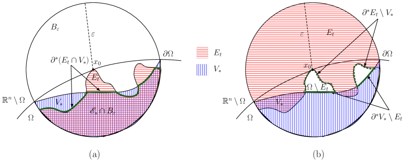
where
see Figure 1(a) below.
Applying these identities to (28) we obtain
| (29) |
On the other hand, let us observe that the set is admissible for problem (5), and furthermore (27) shows that -a.e. Consequently
| (30) |
in light of our convention (7). In particular, the statement can be made more precise by means of the barrier condition of for the minimizer and (30), to read now . Put another way, , so by virtue of the barrier condition once again we see that cannot be a minimizer of (18). Hence, by the characterization (10) of the weighted perimeter and the minimality of , we derive
where we used that in . This inequality can be exploited in light of the identities below:
to simply get
| (31) |
It immediately follows from (29) and (31) that
thus finishing the proof of the contradiction argument in the case .
The other case where is argued again by contradicting the minimality of in (), nonetheless, for the sake of completeness we briefly discuss the proof. Indeed, the continuity of the extension of shows
| (32) |
The claim is that , if we now take . Just as in the previous case we analyze the difference
| (33) |
see Figure 1(b) above.
Let us consider now a new auxiliary set , and perform a similar analysis as before. Noting , from (32) we get which, in addition to (by the barrier condition), implies that . Since is admissible in (), the barrier condition once again yields
leading to the desired conclusion, in view of (33). The proof of Lemma 5.1 is now complete. ∎
Continuing the study of the family we now give a basic geometric description on how they are positioned inside of the domain .
Lemma 5.2.
Suppose satisfies the barrier condition with respect to . Then, for any with , there holds
Proof of Lemma 5.2.
The containment follows from the same argument as in [42]. Let us observe is a competitor with in (),
In a similar fashion, it can be readily seen is a competitor with in . It follows
As the -perimeter satisfies Proposition 2.3, the above inequalities imply . On the other hand, solves the problem thus yielding . We conclude , which in view of our convention (7) then yields
| (34) |
It remains to show that this containment is actually strict. This method uses topological arguments along with techniques from geometric measure theory, and is an adaptation from the proof of this lemma in [42]. Let us start noting
| (35) |
relative to the topology on . In addition, since we observe that Lemma 5.1 implies
| (36) |
In consideration of (34)-(35)-(36) we will prove the statement of this Lemma by showing
For this purpose let us assume on the contrary that . The goal of the remainder of our proof is to verify the points below:
-
(I)
consists of the connected components of that do not intersect .
-
(II)
If denote any connected component of , then has to intersect .
Using the density of in (see (12) in §2), we immediate conclude from (I)-(II) that must be empty, thus reaching a contradiction.
To argue (I) first note that is open relative to , for if , then from and from the fact that both , are -area minimizing in , we can apply the maximum principle Theorem 3.1 to conclude that and must agree on a neighborhood of . On the other hand, is clearly closed relative to , so from (36) we get that every connected component of is disjoint from .
The proof of (II) is based on the fact that is -area minimizing in . This is a rather general fact as given in the following
Lemma 5.3 ([19, Lem. 4.5]).
Let be a bounded Lipschitz domain with connected boundary, and assume is -perimeter minimizing in . If is a connected component of , then .
The proof of Lemma 5.3 is based on topological arguments in geometric measure theory. A full proof can be found in [19], where the authors argue by contradiction that if a set is -perimeter minimizing and admits some component of whose closure is disjoint from , then could have not been -perimeter minimizing in the beginning. ∎
6. Proof of the main Theorem 1.1
We are now in position to build up a continuous solution to the weighted least gradient problem ( LGP). For , we define
| (37) |
Let us observe that is a closed set since every point of is either a regular point of or a point where the tangent cone exists (see §2). This shows that , and so our convention (7) then yields . The latter observation combined with the identity for any sets and the fact that is open, show altogether
therefore , for any . In addition, using the boundary value Lemma 5.1 and topological considerations we can see that for any , there hold
| (38) | |||
| (39) |
Finally, we observe that for any with
| (40) |
relative to . Indeed, topological considerations show that for a.e. , , where denotes the topological boundary relative to the subspace topology of . The validity of (40) is then a mere consequence of Lemma 5.1 and Lemma 5.2 combined.
The definition of our candidate for a solution is the one given below:
| (41) |
The next result asserts that gives rise to a continuous function which meets the boundary condition in the strong sense.
Theorem 6.1.
The proof of Theorem 3.5 in [42] naturally carries over to prove our Theorem 6.1, since it relies solely on (38)-(39), plus some basic topological and analytic considerations.
Finally, let us now restate and provide a proof of our main theorem:
Theorem 1.1.
For , let be a bounded Lipschitz domain with boundary satisfying the barrier condition (5), and let be a non-degenerate weight function in the sense of (2). Then for any boundary data , the function defined in (41) is a continuous solution to
| (42) |
where is understood in the sense of traces of -functions. Furthermore, the superlevel sets of minimize the weighted perimeter measure with respect to competitors meeting the boundary conditions imposed by on .
Proof of Theorem 1.1.
We follow the outline of the proof of Theorem 3.7 in [42]. For any competitor of (42), consider the extension of with in , and let . It is sufficient to show that
| (43) |
since the weighted co-area formula (cf. Proposition 2.2) would then yield
where in the first identity we have used that for all and Theorem 6.1(iii). Let us start arguing (43) by noting for all that , while the set minimizes the -perimeter amongst competitors satisfying this condition. Hence,
or equivalently,
The characterization (10) of the -perimeter measure and the fact that on show that the above inequality reduces to
| (44) |
On the other hand, let us note that Lemma 5.1 implies that the set is -null for a.e. . Indeed, is a -null set for all but countably many , since . From this and (6) we get for a.e. . Thereby, in light of (44), we will have established (43) once we prove
| (45) |
This will be argued in the same way as before, once we are able to prove that
| (46) |
Let us recall is the trace on of admissible in (42), so for -a.e. ,
| (47) |
(cf. [45, §5.14]). Thus in order to prove (46), we consider any as in (47) such that , say with . It follows that
Analogously, as is the trace of , the argument above shows
These two identities above imply
whence , and so . In a similar fashion, we can argue that by means of (47), in light of
which holds for a.e with . The conclusion is , which finishes the proof of Theorem 1.1. ∎
References
- [1] M. Amar and G. Bellettini, A notion of total variation depending on a metric with discontinuous coefficients, Ann. Inst. H. Poincaré Anal. Non Linéaire 11 (1994), no. 1, 91–133.
- [2] F. Andreu, V. Caselles, J.M. Mazón, J.S. Moll, The minimizing total variation flow with measure initial conditions, Commun. Contemp. Math. 6 (2004), no. 3, 431–494.
- [3] F. Andreu, J.M. Mazón, J.S. Moll, The total variation flow with nonlinear boundary conditions, Asymptot. Anal. 43 (2005), no. 1-2, 9–46.
- [4] P. Athavale, R.L. Jerrard, M. Novaga and G. Orlandi, Weighted TV minimization and applications to vortex density models, J. Convex Anal. 24 (2017), no. 4, 1051–1084.
- [5] S. Baldo, R.L. Jerrard, G. Orlandi, and H.M. Soner, Vortex density models for superconductivity and superfluidity, Comm. Math. Phys. 318 (2013), no. 1, 131–171.
- [6] G. Belletini, V. Caselles, M. Novaga, The total variation flow in , J. Differential Equations 184 (2002), no. 2, 475–525.
- [7] E. Bombieri, E. De Giorgi, and E. Giusti, Minimal cones and the Bernstein problem, Invent. Math. 7 (1969), 243–268.
- [8] V. Caselles, G. Facciolo, and E. Meinhardt, Anisotropic Cheeger sets and applications, SIAM J. Imaging Sci. 2 (2009), no. 4, 1211–1254.
- [9] L.C. Evans and R. Gariepy, Measure theory and fine properties of functions, Studies in Advanced Mathematics, CRC Press, Boca Raton, FL 1992.
- [10] H. Federer, Geometric measure theory, Grundlehren Math. Wiss., vol. 153, Springer-Verlag Berlin Heidelberg, 1969.
- [11] D. Gilbarg and N.S. Trudinger, Elliptic partial differential equations of second order, 3rd ed., Grundlehren Math. Wiss., vol. 224, Springer-Verlag Berlin Heidelberg, 1998.
- [12] E. Giusti, Minimal surfaces and functions of bounded variation, Monogr. in Mathematics, vol. 80, Birkhaüser, Boston, 1984.
- [13] W. Górny, Planar least gradient problem: existence regularity and anisotropic case, Calc. Var. Partial Differential Equations 57 (2018), no. 4, 57–98.
- [14] W. Górny, P. Rybka and A. Sabra, Special cases of the planar least gradient problem, Nonlinear Anal. 151 (2017), 66–95.
- [15] R. Hardt and L. Simon, Area minimizing hypersurfaces with isolated singularities, J. Reine Angew. Math. 362 (1985), 102–129.
- [16] H. Hakkarainen, R. Korte, P. Lahti, and N. Shanmugalingam, Stability and continuity of functions of least gradient, Anal. Geom. Metr. Spaces 3 (2015), no. 1, 123–139.
- [17] N. Hoell, A. Moradifam, and A.I. Nachman, Current density impedance imaging of an anisotropic conductivity in a known conformal class, SIAM J. Math. Anal. 46 (2014), no. 3, 1820–1842.
- [18] I.R. Ionescu and T. Lachand-Robert, Generalized Cheeger sets related to landslides, Calc. Var. Partial Differential Equations 23 (2005), no. 2, 227–249.
- [19] R.L. Jerrard, A. Moradifam, and A.I. Nachman, Existence and uniqueness of minimizers of general least gradient problems, J. Reine Angew. Math. 734 (2018), 71–97.
- [20] R. Korte, P. Lahti, X. Li, and N. Shanmugalingam, Notions of Dirichlet problem for functions of least gradient in metric measure spaces, arXiv:1612.06078 [math.AP], 2016.
- [21] R.V. Kohn and G. Strang, The constrained least gradient problem, Non-Classical Continuum Mechanics, Lecture Note Series 122, London Mathematical Society, Cambridge Univ. Press, 1987, pp 226–243.
- [22] P. Lahti, L. Malý, N. Shanmugalingam, G. Speight, Domains in metric measure spaces with boundary of positive mean curvature, and the Dirichlet problem for functions of least gradient, arXiv:1706.07505 [math.AP], 2017.
- [23] J.M. Mazón, The Euler-Lagrange equation for the anisotropic least gradient problem, Nonlinear Anal. Real World Appl. 31 (2016), 452–472.
- [24] M. Miranda, Sulle singularita della frontiere minimali, Rend. Semin. Mat. Univ. Padova 38 (1967), 181–188.
- [25] J.S. Moll, The anisotropic total variation flow, Math. Ann. 332 (2005), no. 1, 177–218.
- [26] A. Moradifam, Existence and structure of minimizers of least gradient problems, arXiv:1612.08400 [math.AP], 2016.
- [27] , Least gradient problems with Neumann boundary condition, J. Differential Equations 263 (2017), no. 11, 7900–7918.
- [28] A. Moradifam, A.I. Nachman and A. Tamasan, Conductivity imaging from one interior measurement in the presence of perfectly conducting and insulating inclusions, SIAM J. Math. Anal. 44 (2012), no. 6, 3639–3990.
- [29] , Uniqueness of minimizers of weighted least gradient problems arising in hybrid inverse problems, Calc. Var. Partial Differential Equations 57 (2018), no. 1, Art. 6, 14 pp.
- [30] F. Morgan, Geometric measure theory: A beginner’s guide, Academic Press, 4th ed., 2009.
- [31] F. Morgan, Regularity of isoperimetric hypersurfaces in Riemannian manifolds, Trans. Amer. Math. Soc. 355 (2003), no. 12, 5041–5052.
- [32] A.I. Nachman, A. Tamasan and A. Timonov, Conductivity imaging with a single measurement of boundary and interior data, Inverse Problems 23 (2007), no 6, 2551–2563.
- [33] , Recovering the conductivity from a single measurement of interior data, Inverse Problems 25 (2009), no. 3, 035014, 16 pp.
- [34] , Current density impedance imaging, Tomography and Inverse Transport Theory, Contemp. Math. Series 559, Amer. Math. Soc., 2011, pp. 135–149.
- [35] A.I. Nachman, A. Tamasan and J. Veras, A weighted minimum gradient problem with complete electrode model boundary conditions for conductivity imaging, SIAM J. Appl. Math. 76 (2016), no. 4, 1321–1343.
- [36] M.Z. Nashed and A. Tamasan, Structural stability in a minimization problem and applications to conductivity imaging, Inverse Probl. Imaging 5 (2011), no. 1, 219–236.
- [37] R. Schoen and L. Simon, A new proof of the regularity theorem for rectifiable currents which minimize parametric elliptic functionals, Indiana Univ. Math. J. 31 (1982), no. 3, 415–434.
- [38] R. Schoen, L. Simon and F.J Jr. Almgren, Regularity and singularity estimates on hypersurfaces minimizing parametric elliptic variational integrals, Acta Math. 139 (1977), no. 3-4, 217–265.
- [39] L. Simon, Lectures on geometric measure theory, Proc. Centre Math. Anal. Austral. Nat. Univ., vol. 3, Canberra 1983.
- [40] , A strict maximum principle for area minimizing hypersurfaces, J. Differential Geom. 26 (1987), no. 2, 327–335.
- [41] G.S. Spradlin, A. Tamasan, Not all traces on the circle come from functions of least gradient in the disk, Indiana Univ. Math. J. 63 (2014), no. 6, 1819–1837.
- [42] P. Sternberg, G.H. Williams, and W.P. Ziemer, Existence, uniqueness, and regularity for functions of least gradient, J. Reine Angew. Math. 430 (1992), 35–60.
- [43] P. Sternberg and W.P. Ziemer, The Dirichlet problem for functions of least gradient, Degenerate diffusions (Minneapolis, MN, 1991), 197–214, in IMA Vol. Math. Appl. vol 47, Springer, New York, 1993.
- [44] B. Solomon, and B. White, A strong maximum principle for varifolds that are stationary with respect to even parametric elliptic functionals, Indiana Univ. Math. J. 38 (1989), no. 3, 683–691.
- [45] W.P. Ziemer, Weakly differentiable functions, Grad. Texts Math., vol. 120, Springer-Verlag, New York 1989.