The RRc stars: Chemical Abundances and Envelope Kinematics

Abstract

We analyzed series of spectra obtained for twelve stable RRc stars observed with the echelle spectrograph of the du Pont telescope at Las Campanas Observatory and we analyzed the spectra of RRc Blazhko stars discussed by Govea et al. (2014). We derived model atmosphere parameters, [Fe/H] metallicities, and [X/Fe] abundance ratios for 12 species of 9 elements. We co-added all spectra obtained during the pulsation cycles to increase $S/N$ and demonstrate that these spectra give results superior to those obtained by co-addition in small phase intervals. The RRc abundances are in good agreement with those derived for the RRab stars of Chadid et al. (2017). We used radial velocity measurements of metal lines and H$\alpha$ to construct variations of velocity with phase, and center-of-mass velocities. We used these to construct radial-velocity templates for use in low-medium resolution radial velocity surveys of RRc stars. Additionally, we calculated primary accelerations, radius variations, metal and H$\alpha$ velocity amplitudes, which we display as regressions against primary acceleration. We employ these results to compare the atmosphere structures of metal-poor RRc stars with their RRab counterparts. Finally, we use the radial velocity data for our Blazhko stars and the Blazhko periods of Szczygieł & Fabrycky (2007) to falsify the Blazhko oblique rotator hypothesis.

1 INTRODUCTION

RRc stars are core helium-burning first overtone pulsators that occupy the blue (hot) side of the RR Lyrae instability strip. They comprise approximately one quarter of the Galactic RR Lyrae population (Drake et al., 2014; Mateu et al., 2012; Soszyński et al., 2014). This estimate is compromised by the lower light amplitudes of RRc stars which tend to decrease frequency estimates, and confusion with WUMa-type contact binaries that tends to increase them. Because they are hotter than the RRab, their metallic lines are weaker, so they were not included in the low resolution spectral abundance survey of Layden (1994), and they are under-represented in extant high-resolution spectroscopic investigations of the RR Lyrae stars (see Chadid et al. 2017 and references therein). The most extensive high resolution abundance study of RRc stars is that of Govea et al. (2014). Early estimates of RRc Luminosity via statistical parallax (Hawley et al., 1986; Strugnell et al., 1986) derived from small samples (n $\sim$ 20) have recently been supplanted by the analysis of Kollmeier et al. (2013) based on a large RRc sample (n = 242) provided by the All Sky Automated Survey (hereafter ASAS, Pojmanski 2002).

The present RRc study is the sixth in a series devoted to pulsational velocities and chemical compositions of RR Lyrae stars from echelle spectra gathered with the Las Campanas Observatory (LCO) du Pont telescope. The observations and reductions are nearly identical in our previous papers: For et al. (2011a, b), Chadid & Preston (2013), Govea et al. (2014)[hereafter GGPS14], and Chadid et al. (2017)[hereafter CSP17]. This information will only be summarized here; see those studies for more detailed descriptions.

In this paper we present abundance analyses and radial velocity ($RV$) measurements of twelve stable RRc stars and the seven Blazhko RRc stars investigated previously by GGPS14. Our results permit comparisons of the abundances and pulsation properties of the RRc stars with those of the RRab sample of CSP17. The basic observations, reductions, radial velocity determinations, spectrum stacking, and equivalent width measurements are presented in §2, 3, and 4. Model atmosphere, metallicity, and abundance analyses are discussed in §5. We explore RRc radial velocity variations in §6 and §7. Finally, we discuss failure of the rotational modulation hypothesis to explain the Blazhko effect in §8.

2 OBSERVATIONS AND REDUCTIONS

The du Pont echelle spectrograph was employed with a 1.5 x 4.0 arcsec aperture which yielded a resolving power $R$ = $\lambda/\Delta\lambda$ $\sim$ 27000 at 5000 Å. The complete spectral domain was $\lambda\lambda$ 3400–9000, with small wavelength gaps in the CCD order coverage appearing at $\lambda$ 7100 Å and growing with increasing wavelength. Table 1 contains basic data on these stars and those studied by GGPS14.

Twelve stable RRc stars were chosen from the brightest RRc stars in the ASAS catalogue that were conveniently observable at LCO during our assigned nights. A total of 615 echelle observations were obtained during six nights in March 2014 and three nights in September 2014. Complete or almost complete phase coverage of the pulsations cycles was achieved for seven of the twelve stars. All twelve stars were observed at or near mid-declining light where line broadening is characteristically most favorable for spectroscopic analysis.

The pulsational periods of our program stars lie in the range 0.24 $\lesssim$ $P_{ASAS}$ $\lesssim$ 0.38 days, with visual light amplitudes 0.23 $<$ $V_{amp;ASAS}$ $<$ 0.55 (Table 1). In order to avoid deleterious effects of phase smearing, the maximum spectroscopic integration time was 400 s, with some observations as short as 200 s. The maximum exposure times were thus less than 3% of the shortest program star period. This led to negligible $RV$ variations during the individual stellar observations. The short exposures, apparent magnitudes the targets, and the modest du Pont telescope aperture (2.5 m), led to low signal-to-noise in the extracted spectra, typically $S/N$ $<$ 20.

Observations of the stars discussed previously by GGPS14 were obtained in 2009 and 2010, as circumstances permitted during our RRab survey (CSP17). Their spectra were gathered in order to test the hypothesis that Blazhko periods are axial rotation periods, so the GGPS14 stars form a strongly biased Blazhko sample. Because of the relative rarity of Blazhko variables, the average visual magnitude of this sample at minimum light, $\langle V_{min}\rangle$ = 11.7, is more than one magnitude fainter than that of our stable RRc sample, $\langle V_{min}\rangle$ = 10.5. Therefore, of necessity, integration times were longer than those employed for the RRab stars in CSP17: the maximum was 1200 s, with typical values less than 900 s. Fortunately, the $RV$ amplitudes of RRc stars are smaller by a factor of about two than those of RRab stars, so line broadening due to changing $RV$ during these longer integrations remained unimportant. Finally, because the Blazhko stars were observed at brief, randomly chosen times during the RRab survey, phase coverage for them is markedly inferior to that obtained for our stable RRc stars. We will discuss the axial rotations of the Blazhko sample in §8.

We extracted spectra from the original CCD image files using procedures discussed previously (Preston & Sneden, 2000; For et al., 2011a); for the most part the description of these reduction steps need not be repeated here. However, as discussed in CSP17 we used one shortcut in scattered light removal. Our reduction steps do not explicitly account for scattered light, and in §3.1 of For et al. (2011a) there is detailed consideration of its contribution to the total flux in the extracted du Pont echelle spectra. Fortunately, scattered light accounts for a near-uniform 10% of the light in the spectral orders of interest to our work. Therefore, like CSP17 we simply subtracted the 10% and renormalized to get the final spectra ready for analysis.

3 RADIAL VELOCITIES

We accumulated $\sim$50$\pm$15 spectra for each stable RRc. These allow us to examine $RV$ variations of the metallic lines and H$\alpha$ with pulsation phase and to compare the relationship between velocity amplitude and light amplitude of first overtone pulsators with that established for the RRab fundamental pulsators. Likewise, we can compare the envelope structures revealed by the different $RV$ variations of the near-photospheric metal line velocities and the velocities at the very small continuum optical depths high in the atmosphere where the core of H$\alpha$ is formed.

As done for the RRab sample, we flattened and stitched together thirteen echelle orders of each spectrum spanning the wavelength interval $\lambda\lambda$4000$-$4600 Å by use of an IRAF script prepared by Ian Thompson (private communication). This is the same spectral interval used in our previous papers. Flattened, normalized spectra of the echelle order containing H$\alpha$ near its center were used to measure H$\alpha$ radial velocities. As in our previous investigations we measured $RV$s with the $IRAF/fxcor$ package, using the same reference spectra for metal lines (star CS 22874-009) and for H$\alpha$ (CS 22892-052), and the same primary $RV$ standard (HD 140283). We used the same Gaussian fitting function to locate line centers as discussed in detail by CSP17, and the same procedure for measurement of occasional asymmetric H$\alpha$ cores. That is, if an H$\alpha$ core is asymmetric we always fit a Gaussian to the flux minimum and the steepest wing of the profiles. Thus, our $RV$s for RRc stars are directly comparable to those reported previously for the RRab stars by CSP17. The derived $RV$s for metallic lines and H$\alpha$ are given in Table 2.

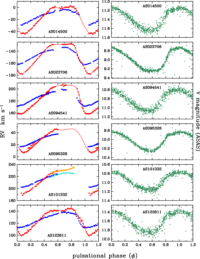
Figure 1: Left-hand panels: Derived $RV$s for metal lines (blue points) and H$\alpha$ (red points and mean line) as functions of pulsational phase $\phi$ for the first six of the stable RRc stars newly observed for this study. the $RV$ extent of each panel is 60 km s^-1, approximately centered on the stellar systemic velocity. Right-hand panels: ASAS database $V$ magnitudes for these stars. The $P$ and $T_{0}$ values to produce these light curves are those derived from the $RV$ analyses of this study. For AS101332 the $RV$ data do not match well even though the observations were obtained only two nights apart (Table 2). We show this by using turquois color for the metal line and orange color for the H$\alpha$ points in this star’s $RV$ plot.

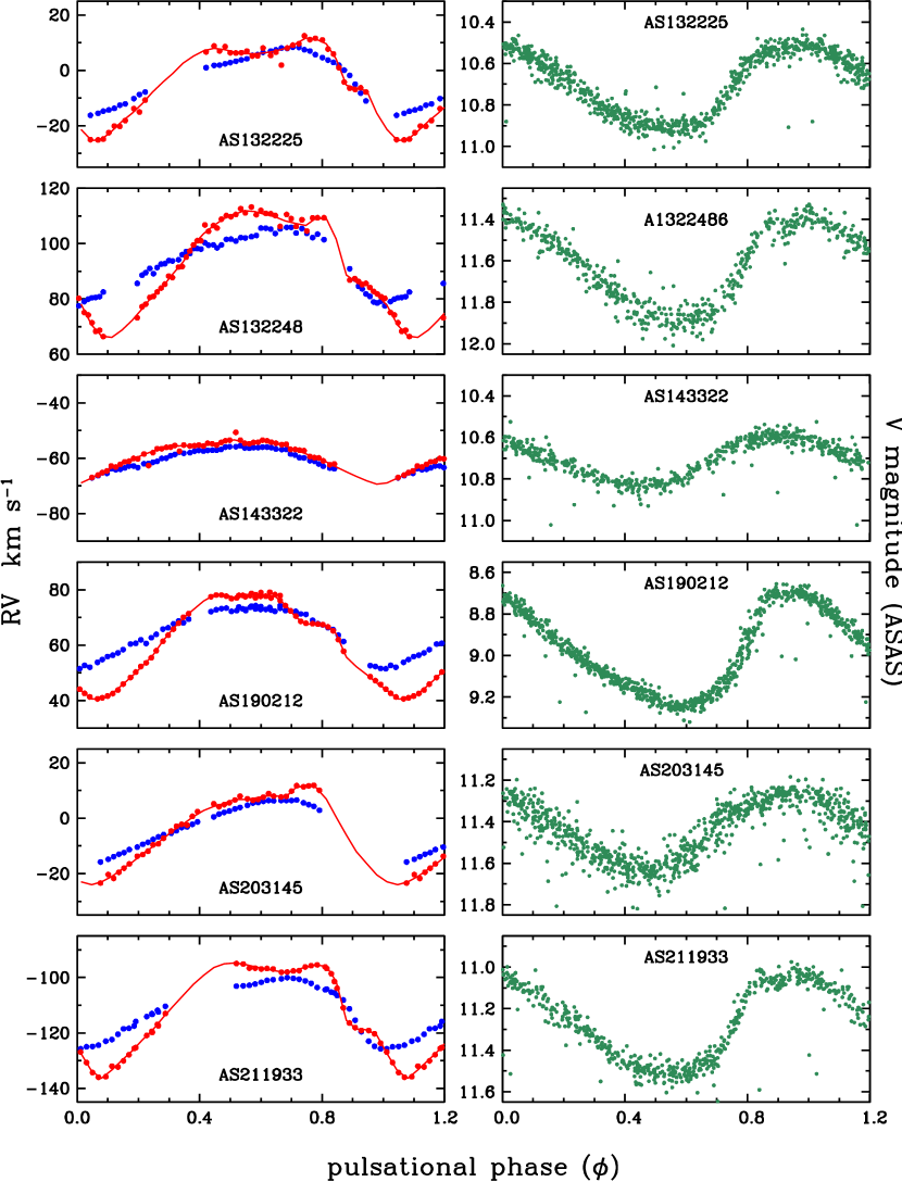
Figure 2: Velocities and $V$ magnitudes as functions of pulsational phase $\phi$ for the second set of six stable RRc stars of this study. All points and lines are as in Figure 1.

Plots of $RV$ versus pulsation phase were computed for the twelve stable RRc stars by use of ASAS periods and initial Heliocentric Julian Days listed in Table 1. These curves are shown in the left-hand panels of Figures 1 and 2. The $RV$ curves for the GGPS14 stars are shown in their paper.

We adopted zero points of phase for our radial velocity curves and ASAS visual light curves by requiring that the minima of visual magnitudes and radial velocities be coincident. Such coincidence, first noticed by Sanford (1930) for two classical cepheids, is verified for RR Lyrae stars by data in Table The RRc stars: Chemical Abundances and Envelope Kinematics that we constructed from examination of near-contemporaneous radial velocity and visual photometric observations made by several groups for applications of the Baade-Wesselink method. A definitive investigation of coincidence among the RR Lyrae stars of M3 (not attempted here) could be conducted by use of the recent elegant observations of Jurcsik et al. (2015, 2017). Table The RRc stars: Chemical Abundances and Envelope Kinematics provides arguable evidence for small offsets ($\simeq$0.01P) for both RRab and RRc stars, but these do not exceed their standard deviations. We are obliged to assume coincidence because, unfortunately, the ASAS photometric ephemerides of our stars do not predict our observed times of minimum $RV$. Our spectroscopic observations, all made near JD 2456800 $\pm$ 100, were obtained some 1600 days or 5000 pulsation cycles after the most recent published ASAS photometry (through Dec. 31, 2009), so we suspect unidentified problems with the published light curve ephemerides. The ASAS release of photometric data from 2010 forward is a work in progress, so we can expect resolution of this ephemeris problem in the near future. In the present study we arbitrarily adopted values of $HJD0$ that produced visual light maxima near phases 0.00, consistent with the results in Table The RRc stars: Chemical Abundances and Envelope Kinematics. We also made small adjustments to the ASAS period values to produce light curves with the most internal consistency. We show these light curves in the right-hand panels of Figures 1 and 2. See GGPS14 for light curve plots of the Blazhko stars.

Note that our radial velocity observations of AS101332 made on JD 2456740 and 2456742 do not superpose well; see Figure 1. Were this to be a Blazhko phenomenon the Blazhko period would have to be short and the amplitude of the phase variation would have to be large. We see no evidence of this in the ASAS photometry, and the star was not identified as a Blazhko variable by Szczygieł & Fabrycky (2007). We offer no other explanation for the behavior of this star.

The eight stable RRc stars (those in column 7 of Table 1 for which we can estimate $RV$ amplitudes) comprise a homogeneous group with respect to radial velocity and visual light amplitudes (24.2 $\pm$ 5.1 km s^-1, and 0.46 $\pm$ 0.09 mag., respectively). If we omit the low amplitude outlier AS143322, the standard deviations are even smaller ($\pm$2.3 km s^-1 and $\pm$0.05 mag, respectively). We used our estimates of the extrema defined by the data in Figures 1 and 2 to calculate the visual light and radial velocity amplitudes listed in columns 7 and 8 of Table 1; these will be discussed in §6.

Our small log g = 2.3 for AS143322 rules out classification as an SX Phe star like those studied Nemec et al. (2017). The small [Fe/H] = $-$1.48 of this star rules out identification as a $\delta$ Scuti star, so perforce we retain AS143322 as an unusual short-period, low-amplitude RRc (Table 1).

4 PHASE CO-ADDITION AND EQUIVALENT WIDTHS

To perform model atmosphere and chemical composition analyses we again re-stitched and flattened all of the echelle orders in each observed spectrum, taking care in these procedures to excise anomalous cosmic rays and other radiation events, to produce continuum-normalized spectra ready for equivalent width measurements. The spectra also were corrected to zero velocity using the instantaneous velocity shift for an observation that was derived as part of the computations discussed in §3. However, the combination of RRc line strengths and the constraints of our observational parameters necessitated further manipulations to produced useful spectra for atmospheric analysis.

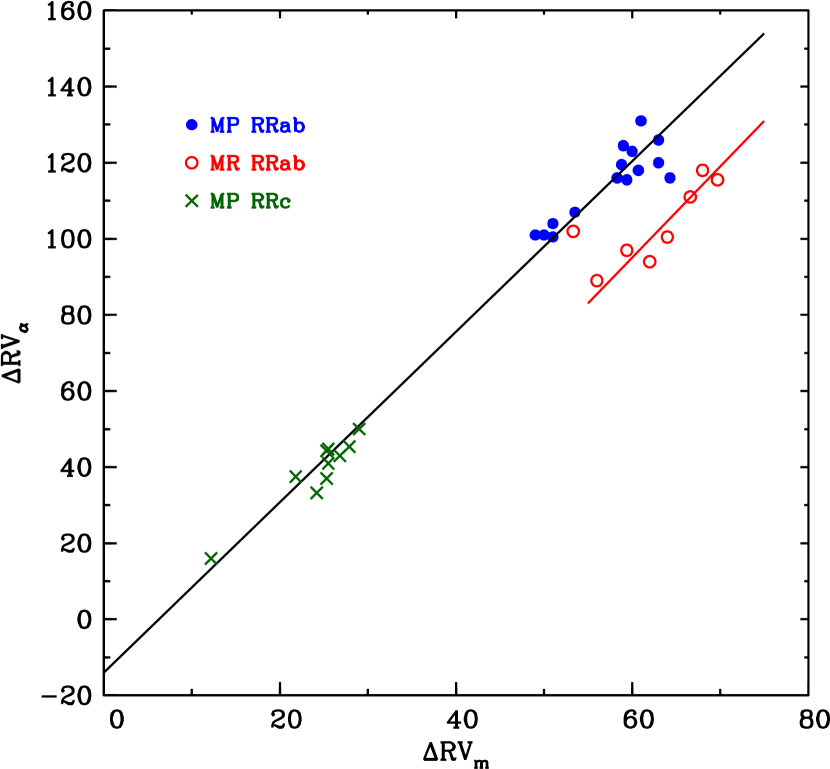
Figure 9: H$\alpha$ $RV$ amplitude $\Delta RV_{\alpha}$ plotted versus metallic radial velocity amplitude $\Delta RV_{m}$. Point types and colors for the MP RRab and MP RRc stars are in Figure 8; the red open circles are for MR RRab stars. The lines represent linear regression fits to the MR RRab data (red), and the the combined MP RRab and MP RRc data.

Average RRc parameters reported by GGPS14 were T_eff $\sim$ 7200 K, log g $\sim$ 2.3, and [Fe/H] $\sim$ $-$2.0. Such very warm and metal-poor giant stars have weak-lined spectra. The modest $S/N$ of our individual short-exposure spectra of RRc stars were ill-suited to derivation of model atmosphere quantities and abundances of individual elements. The most reliable stellar abundances usually arise from equivalent width ($EW$) measurements of weak absorption features that lie on the linear part of the curve-of-growth, that is lines that have reduced widths log($RW$) = log($EW/\lambda$) $<$ $-$5.0 (e.g., 45 mÅ at $\lambda$ = 4500 Å). Such lines are sometimes detectable on our individual spectra but their measured $EW$’s have large uncertainties. We illustrate this problem in Figure 3. The top spectrum in this figure is one integration of the star AS162158, one of the most metal-poor stars of our sample. Many absorption lines of (mostly) Fe-group ionized species are in this spectral region, but nearly all of them have $EW$ $\lesssim$ 80 mÅ, or log($RW$) $\lesssim$ $-$4.7. It is clear from inspection of this Figure 3 “snapshot” spectrum of AS162158 that $EW$s of weak detected lines are very uncertain. Figure 9 of GGPS14 shows another example, that of the more metal-rich AS230659, in the 5200 Å spectral region where the stellar fluxes are higher. Even in this case $EW$ values for weak lines are not easy to determine on individual spectra.

Therefore, following the technique developed by For et al. (2011b), we co-added individual spectra in phase bins no wider than $\delta\phi$ = 0.1, producing higher $S/N$ spectra representative of several phase intervals throughout our program star pulsational cycles. In Table 4 we list all phase bins for each program star, the mean phase of the bins and the number of individual spectra contributing to the mean spectra. An example of the spectrum phase averaging is given in the middle spectrum of Figure 3; the increase in $S/N$ by the co-addition of three AS162158 spectra obtained near $\phi$ = 0.35 is apparent. Hereafter these will be called “phase-mean” spectra for each star.

Even these co-additions were insufficient to reveal very weak features. This did not severely affect our analyses of species with many transitions on our spectra, such as Fe i, Fe ii, and Ti ii. But many species of interest, e.g., Cr i or Ba ii, are represented by only very few lines; these species often cannot be studied in our more metal-poor RRc stars, even with phase co-added spectra. Fortunately RRc stars have relatively mild atmospheric physical state changes during their pulsation cycles. The mean ranges of temperatures and gravities of the program stars to be discussed in §5 are $\langle\mbox{T${}_{\rm eff}$}_{,max}-\mbox{T${}_{\rm eff}$}_{,min}\rangle$ = 540 $\pm$ 250 K and $\langle\mbox{log~{}{\it g}}_{,max}-\mbox{log~{}{\it g}}_{,min}\rangle$ = 0.7 $\pm$ 0.5 . Therefore we also performed co-additions of all spectra for each program star. This procedure of course threw away all pulsational phase information, in return for greatly increased $S/N$. These spectra were then analyzed for stellar parameters and abundance ratios. The bottom spectrum in Figure 3 shows the result of co-adding all 21 spectra of AS162158. Hereafter these will be called “total” spectra for each star.

We performed $EW$ measurements with the recently-developed $pyEW$ code This $EW$ package is a Python script that, for a given stellar absorption line, fits a multigaussian function to a fragment of the spectrum centered on the line under examination. The multigaussian approach allows one to handle complex features that included in blending contaminants. The $pyEW$ code can be used in a completely automatic way, or it can be run in interactive mode which allows to user to modify a solution that was found automatically. It can be used in a hybrid fashion in which some of the lines are analyzed automatically and others are subjected to user scrutiny.

5 Atmosphere and Abundance Derivations from the Spectra

We determined atmospheric parameters (T_eff, log g, $\xi_{\rm t}$, [Fe/H]) and ratios [X/Fe] for our RRc stars with essentially identical procedures to those used by CSP16 for their sample of RRab stars. Here we summarize the CSP17 procedures, mostly as described in their §3.1. At the end of this section we comment on the metallicity range of our RRc stars.

5.1 Model Atmosphere Parameters

Model atmospheres were interpolated in the Kurucz (2011) ATLAS grid and we employed a new version of the local thermodynamic equilibrium (LTE) line analysis program $MOOG$ (Sneden, 1973) to derive abundances for individual lines. The $pyMOOGi$ code is a Python “wrapper” that retains the basic synthetic spectrum computations of $MOOG$ but introduces improved interactive graphical capabilities through standard Python library functions. Currently $pyMOOGi$ is available for the synth and abfind $MOOG$ drivers that we need in this study. We adopted the CSP17 atomic line list without change.

The input model atmospheres were iteratively changed until the ensemble of Fe i and Fe ii lines showed no elemental abundance trends with excitation energy $\chi$, line strength log($RW)$, and ionization state, and the input “$\alpha$-enhanced” model metallicity matched the derived [Fe/H] value. We generally discarded very strong lines in our abundance analyses, those with log($RW$) $>$ $-$4.5 ($EW$ $\simeq$ 140 mÅ at 4500 Å). The strengths of those lines increase sharply with increasing log($RW$), clearly reflecting outer atmosphere conditions in pulsating RRc stars that are not well described by our simple plane-parallel atmosphere and LTE line analysis assumptions. The derived model atmosphere and metallicity values for all stars in all co-added phase bins are given in Table 4. These quantities were then averaged on a star-by-star basis to form phase-means values for each of the 19 program stars. These are entered in Table 5.

For each star we also performed the model atmospheric analysis using the total spectra. In Table 6 we list the results. Abundances of other elements were derived from each phase-mean spectrum and each total spectrum, but we deem only those from the total spectra to be reliable enough for further study.

The entries in Table 6 can compared to the phase-mean values of Table 5. Note especially the increase in the number of transitions available for determining the abundances from Fe i and Fe ii lines. As an example of the improvement in ability to measure useful spectral lines by averaging all observations of a star to produce a total spectrum, we show in Figure 4 the line-by-line abundances for Fe in AS162158. In panel (a) we have selected the results for phase $\phi$ =0.632, which is based on co-addition of 3 individual observations, and in panel (b) the results of the total spectrum with co-addition of all 21 observations are shown. The decrease in line-to-line scatter in the analysis of the total spectrum is clear by visual inspection, and confirmed by the statistics of Tables 4 and 6. From the $\phi$ = 0.632 spectrum analysis $\sigma$(Fe i) = 0.28 from 16 lines and $\sigma$(Fe ii) = 0.33 from 13 lines, while from the total spectrum analysis $\sigma$(Fe i) = 0.19 from 22 lines and $\sigma$(Fe ii) = 0.15 from 17 lines.

The metallicities of phase-mean and total spectra correlate well, as can be seen in panel (a) of Figure 5. The mean metallicity offset, $\langle$[Fe/H]${}_{total}-$[Fe/H]${}_{phasemean}\rangle$ = $-$0.08 $\pm$ 0.04 ($\sigma$ = 0.17, 19 stars). The small offset lies well within the star-to-star scatter. If the offset is real then the higher $S/N$ of the total spectrum might be the cause, as the continuum setting becomes easier as the $S/N$ increases. However, the total spectrum is an average over all phases of an ever-changing RRc target, and thus smears the phase-specific information that is available in the phase-mean spectra of a star. Further investigation of this small offset is beyond the scope of our work, and it is clear that all of our methods of deriving RRc [Fe/H] values yield essentially the same answers over a 2-dex metallicity range.

Program star AS190212 deserves comment for several reasons. (1): It is one of the most metal-poor stars of our sample. (2): From its total spectrum we derive an unusually high surface gravity (log g = 3.7; Table 6). (3): Its H$\alpha$ $RV$ curve has a “standstill” flat portion in the phase range $\phi$ $\simeq$ 0.70$-$0.85 (Figure 2) that is not obvious in any of our other RRc stars. AS190212 under its variable star name of MT Tel has several literature metallicity estimates: [Fe/H] $\sim$ $-$2.5 (Przybylski 1983, from a “coarse analysis” with respect to a Hyades cluster star); [Fe/H] = $-$1.63 (Solano et al. 1997, based on two Fe ii lines); and [Fe/H] = $-$1.85 (Fernley et al. 1998, using a $\Delta S$ calibration from Fernley & Barnes 1997). No previous extensive high-resolution spectroscopic analysis of AS190212 has been published. Our analysis of this star was conducted in an identical manner to the others of our sample, and the derived metallicities from Fe i and Fe ii lines of the phase-averaged spectra (Table 5) agree well with those of the total spectra (Table 6). The gravity value was derived from a Saha equilibrium balance between 20 Fe i and 10-13 Fe ii lines. Additionally, the gravity we derive from the AS190212 is not unusually high: log g = 3.2.

The relatively large gravity of AS190212 places it not far from the blue metal-poor (BMP) main sequence studied by Preston & Sneden (2000). Their atmospheric analyses of Du Pont spectra of nearly 50 slowly rotating BMP stars yielded $\langle\mbox{log~{}{\it g}}\rangle$ $\simeq$ 4.3, with only three of their stars having log g $\leq$ 3.9. The atmospheric parameters of AS190212 are similar to those of metal-poor SX Phoenecis stars that exist in small numbers in the halo field (e.g., Preston & Landolt 1999) and in globular clusters (e.g., M53, Nemec et al. 1995). However, SX Phe variables typically have very short periods, $P$ $\sim$ 0.04 days, while the period of AS190212 is 0.32 days. This probably negates association of this star with the SX Phe class. Another intriguing possibility is that AS190212 might be like the mass-transfer binary star OGLE-BLG-RRLYR-02792, whose brighter primary has a very low mass ($M$ = 0.26$M_{\odot}$) star that exhibits RR Lyrae photometric variations (Pietrzyński et al., 2012). Those authors suggest that the complex history of this binary has placed it for a short time in the instability strip domain of the RRc stars. However, while the OGLE primary has about the right temperature, T_eff $\simeq$ 7300 K, its pulsation period is 0.63 days, about double the periods of our RRc sample. AS190212 most likely remains a true RRc star, but one should keep in mind the difficulty in assigning variability classes to stars in this T_eff-log g domain.

5.2 Elemental Abundances

For the total spectra we also derived abundance ratios [X/Fe] from 12 species of 9 elements. The star-by-star values and overall species means are listed in Tables 7 and 8. To compute these [X/Fe] numbers we adopted the recommended solar photospheric abundances of Asplund et al. (2009), and used the same species in numerator and denominator of the fractions, e.g. the [Ti/Fe]_I value was determined from the [Ti/H]_I and [Fe/H]_I abundances, and [Ti/Fe]_II was from [Ti/H]_II and [Fe/H]_II abundances. Many of species in these tables are represented by only a handful of lines, only one in the case of Si i. Obviously the abundances of these species should be viewed with caution.

We derived abundances from six species of four $\alpha$ and $\alpha$-like elements; these are listed in Table 7. There are enough Ti ii lines to make a comparison between the phase-mean and the total spectra. In panel (b) of Figure 5 we show the [Ti/Fe] differences between these two abundance approaches, and they are obviously small. As defined in the figure legend, $\langle\Delta$[Ti/Fe]$\rangle$ = $+$0.04 $\pm$ 0.02 ($\sigma$ = 0.10, 19 stars). As with the metallicity comparison, the total and phase-mean spectra yield the same values for Ti/Fe ratios.

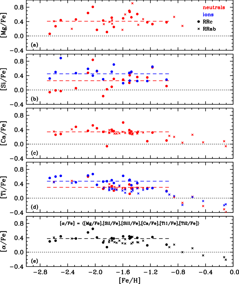
Figure 6: Relative abundance ratios [X/Fe] for the $\alpha$ and $\alpha$-like elements. The colors and point types are defined in the legend of panel (a). The RRc stars are results from the present study, and the RRab stars are those of CSP17. The dished lines in each panel are the overall species mean [X/Fe] values. In panel (e) we show unweighted means of the species abundance from panels (a)-(d), as defined in the panel (e) legend.

In Figure 6 we plot our $\alpha$-element abundances and those of RRab stars studied by CSP17. The line-to-line and star-to-star scatters are larger for Mg (panel a) and Si (panel b) than they are for Ca (panel c) and Ti (panel d). Mg is represented only by a few Mg i lines that are often strong and thus affected by microturbulent velocity choices. Si i has only one routinely detectable transition at 3905 Å. This transition is known to yield unreliable Si abundances (e.g., Sneden & Lawler 2008). Several Si ii lines are available for analysis, but it is difficult to calibrate them because they usually are unreported in the vast majority of metal-poor (typically cooler) stars. In panel (e) we show a simple straight mean for all the $\alpha$ species abundances. These values are essentially invariant across our entire RRc metallicity domain.

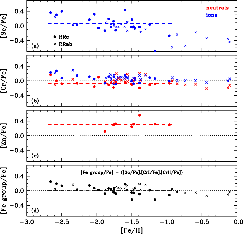
Figure 7: Relative abundance ratios [X/Fe] for Fe group elements. The colors, symbols, and lines are as in Figure 6. In panel (d) we show unweighted means of the species abundances from panels (a) and (b) only; the uncertain [Zn/Fe] abundances of panel (3) are not included.

We also derived abundances from four species of three Fe-group elements beyond Fe itself. These are listed in Table 8 and displayed in Figure 7. Abundances deduced from the 1-2 Zn i lines (panel c) are few in number and we do not consider them to be reliable. The Fe-group means excluding Zn are shown in panel (d) of this figure; they clearly have small star-to-star variations and are consistent with [Fe group/Fe] $\simeq$ 0 over the whole metallicity regime.

Finally, the only $n$-capture elements with reliable abundances derivable over the whole metallicity range are Sr and Ba. These elements have the only strong transitions beyond the near-UV: Sr ii 4077 and 4215 Å, and Ba ii 4554, 5853, 6141, and 6496 Å. However, the Sr ii lines are often very saturated or otherwise compromised in their complex spectral regions, so we only quote Sr abundances for 12 of the 19 program stars in Table 8. The star-to-star scatter for [Sr/Fe] is large, $\sigma$ = 0.50). Caution is warranted in interpretation of our results for both Sr and Ba, but there is little evidence for departures from [Sr,Ba/Fe] = 0 in our data; more detailed $n$-capture analyses for RRc stars would be welcome in the future.

6 PHOTOSPHERIC MOTION PARAMETERS

6.1 Amplitude Diagrams

We combine the RRc photometric and $RV$ amplitudes of this study (Table 1) with those for RRab stars in Table 4 of CSP17, and those for the variables in M3 recently investigated by Jurcsik et al. (2015, 2017) to produce Figure 8. Regression lines through the origin ($\Delta V$ = 0.019$\Delta RV$) for RRc stars, linear ($\Delta V$ = 0.033$\Delta RV$ $+$ 0.934) for the RRab stars. and non-linear power law ($\Delta V$ = 0.011$\Delta RV$ + 2.300$\times 10^{-17}\Delta RV^{9}$) for the M3 observations of Jurcsik et al. provide an observational picture of the different ways that fundamental and first overtone pulsations grow/vanish near the origin.

Similarly, we correlate the RRc metal and H$\alpha$ $RV$ amplitude data, $\Delta RV_{m}$ and $\Delta RV_{\alpha}$, for RRc and RRab stars to produce Figure 9. The slopes of the MP and MR (metal-rich) regressions are similar, as in the preceding figure. We discuss these correlations further in §7.

6.2 Radial Velocity Templates

Low-resolution spectroscopic surveys provide important data about the density and kinematic structure of our Galaxy and its satellites. Single observations of RR Lyrae stars with low-to-moderate spectral resolution can provide radial velocity accuracy ($\pm$5 to 10 km s^-1) that is adequate for these purposes. However, the sizable $RV$ amplitudes of RR Lyrae stars during their pulsation cycles require special treatment (see Kollmeier et al. 2013 for detailed discussion). If accurate photometric elements are available one may infer the center-of-mass velocity ($RV_{CoM}$) from the photometric phase of the observation by use of a velocity template. The template provides a correction that converts an observed $RV$ to $RV_{CoM}$. Such templates have been provided for the metallic line $RV$s of RRab stars by Liu (1991). More recently Sesar (2012) provided templates for RRab stars based on Balmer lines for use with low resolution spectra.

The template correction procedure requires a photometric ephemeris, and it assumes a universal phase relation between times of light maximum and $RV$ minimum; for RRab stars the relationship is coincident at the $\pm$0.01$P$ level. As noted in §3 we cannot verify this coincidence for our RRc sample. We proceed with construction of templates in the expectation that a universal phase relation between light and velocity variations of the RRc stars will be forthcoming. Absent such a universal relation, there is no use for templates.

Omitting outlier AS143322, the remaining eight stable RRc stars in our sample comprise a homogeneous group with respect to visual light amplitude as discussed in §3, so we thought it sufficient to create a single, scalable template for the metal lines of metal-poor RRc stars. In view of the significantly different behavior of H$\alpha$ radial velocity we created a separate template for H$\alpha$. For the metal template we selected the seven stars with reasonably complete $RV$ phase coverage: AS023706, AS094541, AS123811, AS132225, AS132448, AS190212, and AS211933 (see Table 1 and Figures 1 and 2). We omitted AS143322, whose pulsation amplitudes are much smaller than all others in our sample. For the H$\alpha$ template we also removed AS190212 because of the strange behavior of H$\alpha$ during rising light, and we added AS014500.

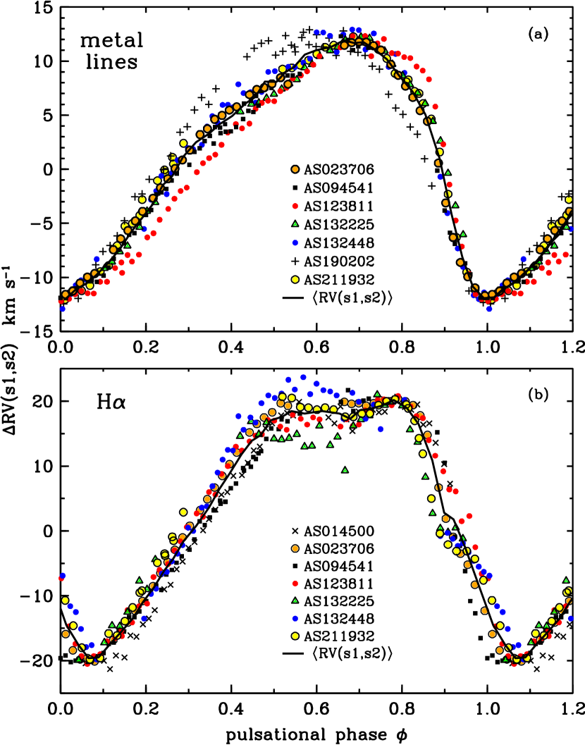
Figure 10: Stretched and shifted $RV$ variations for selected program stars as functions of their pulsational phases. Individual measurements for each star are coded by symbols in the legends for metal lines (panel a) and H$\alpha$ (panel b). The solid black curves represent average values calculated as described in the text. See the text for discussion of the stretching and shifting procedures.

We superposed the metal $RV$ data for these stars, stretching/compressing measured $RV$ variations to two standard amplitudes, $\Delta RV$ = 24 km s^-1 and 30 km s^-1, by use of a scale factor s1, which we centered on $RV$ = 0.0 km s^-1 by use of a shift s2. The values of s1 and s2 that we used are given in Table 9. $RV$(s1,s2) denotes velocities created in this manner. The $RV$(s1,s2) data for $\Delta RV$are displayed in panel (a) of Figure 10, where various colored symbols are used to identify the contributions of each star. We define an average metal velocity variation for the RRc stars as follows. All the data values in Figure 10 were sorted in order of increasing phase. Then average values of phase and $RV$(s1,s2) were calculated in bins of 10 successive values. The average phase interval between successive average values $\langle RV$(s1,s2)$\rangle$ produced by this procedure was $\Delta\phi$ = 0.026 $\pm$ 0.003. These are displayed by the continuous black curves in the figure.

It is evident from panel (a) of Figure 10 that individual stars depart systematically from average metal line $RV$ behavior: the trend for AS190212, the most metal-poor star in our sample, is a conspicuous example. Departures of its $RV$(s1,s2) values from the mean curve as large as 5 km s^-1 occur during about one third of its pulsation cycle. For most of the sample the deviations are much smaller. In view of the characteristic magnitudes of space motions and dispersions of Galactic RR Lyrae stars ($\sim$100 km s^-1), we believe our mean relations provide a satisfactory way to convert individual $RV$ observations to $RV_{CoM}$ values for many purposes.

An identical procedure was used to create the diagram for H$\alpha$ in the panel (b) of Figure 10. This diagram serves to call attention to the definition of the H$\alpha$ $RV$ amplitude, which we calculate as the difference between the $RV$ minimum that occurs near phase $\phi$ $\sim$ 0.1 and the local velocity maximum near $\phi$ $\sim$ 0.8. Data superposed in this manner produce a large range in a second local $RV$ maximum that occurs near $\phi$ $\sim$ 0.5. We only note here that this secondary maximum has a morphological counterpart in the $RV$ curves of RRab stars near phase $\phi$ $\sim$ 0.7 (CSP17). For some stars this maximum is larger (e.g., AS132448 and AS211933) than the one near $\phi$ $\sim$ 0.8.

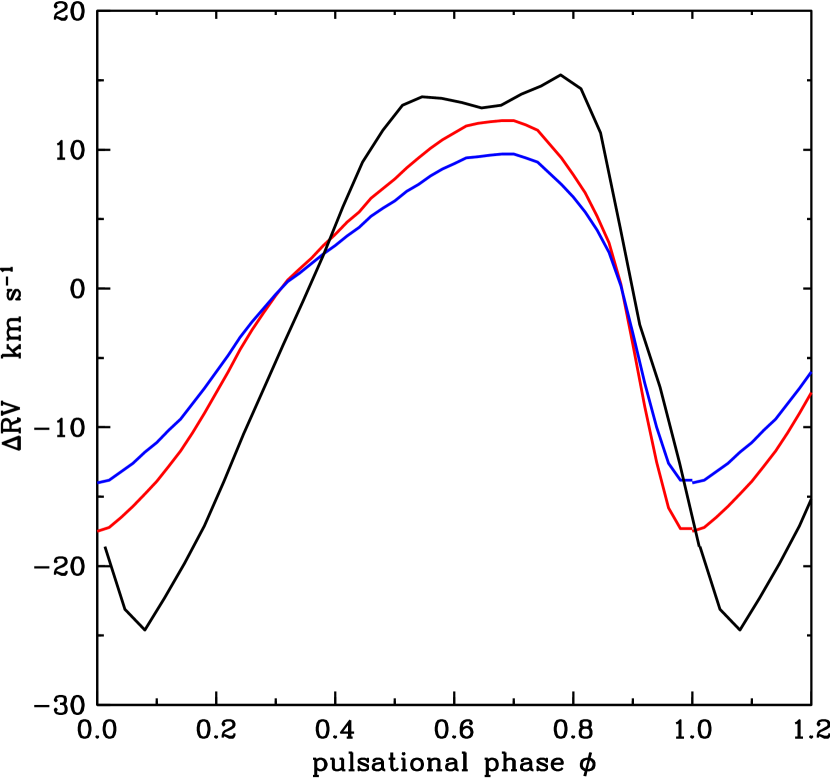
Figure 11: Mean $RV$ variations for metal lines (red and blue curves) and H$\alpha$ (black curve) derived from the data of Figure 10.

We converted the mean $\langle RV$(s1,s2)$\rangle$ curves to templates by calculating the time-averaged values of these curves and shifting the zero points of the velocity scales to produce template velocity corrections. The results of these calculations are presented in Table 10 and displayed in Figure 11. In this table we tabulate $\Delta RV$ = $RV(\phi$) $-$ $RV_{CoM}$, the correction to be subtracted from a radial velocity observed at phase $\phi$. The tabulated corrections can be scaled to any amplitude. The time-averaged $RV$ of any template scaled in this manner remains 0.0 km s^-1. In Figure 11 we show templates for metal line $RV$ amplitudes 24 km s^-1 (blue line) and 30 km s^-1 (red line). These curves bracket the range of $\Delta RV$ possibilities in our sample. We also draw a black line with $RV$ amplitude 40 km s^-1 for the typical variation of H$\alpha$ lines.

7 H$\alpha$ AND METALLIC-LINE VELOCITY VARIATIONS

7.1 Photospheric Dynamics

We used the metallic radial velocity data for the twelve stable RRc stars displayed in Figures 1 and 2 to calculate pulsation velocities, center-of-mass ($\gamma$) velocities, radius variations, and primary accelerations (those that occur during primary light rise; see CSP17).

From the heliocentric radial velocity $RV(\phi)$, we calculate the pulsation velocity dR/dt($\phi$) in the stellar rest frame using: d$R$/d$t(\phi$) = $-p(RV(\phi)-RV_{\gamma}$), where $p$ is the value of the correction factor for geometrical projection and limb darkening and $RV_{\gamma}$ is the center-of-mass velocity. Because the metallic absorption lines are formed near the photosphere, the pulsation velocity d$R$/d$t(\phi)$ is close to the photosphere motion and $RV_{\gamma}$ is assumed to be equal to the so-called $\gamma$-velocity, i.e., the average value of the heliocentric radial velocity curve over one pulsation period. The use of this approximation is discussed by Bono et al. (1994). Here, we use $p$ = 1.36 from Burki et al. (1982) supported by recent studies (Neilson et al., 2012; Ngeow et al., 2012).

The pulsational velocities derived from metal lines are very nearly those of the photosphere: the metal line forming region at $\tau_{5000\AA}$ = 0.15 lies only $\sim$4 km above the photosphere of a Kurucz (2011) model with the characteristic parameters of an RRc atmosphere (T_eff = 7250 K, log g = 2.5).

Radius and acceleration curves were computed from the integrals and derivatives of the pulsational velocity curves, respectively. During pulsation cycles (0 $<$ $\phi$ $<$ 1) gaps in the data were interpolated linearly. In order to minimize the noise, the raw radial velocity curves were convoluted with a sliding window of $\Delta$$\phi$ = 0.1 width. Table 11 contains a summary of these photospheric motion parameters.

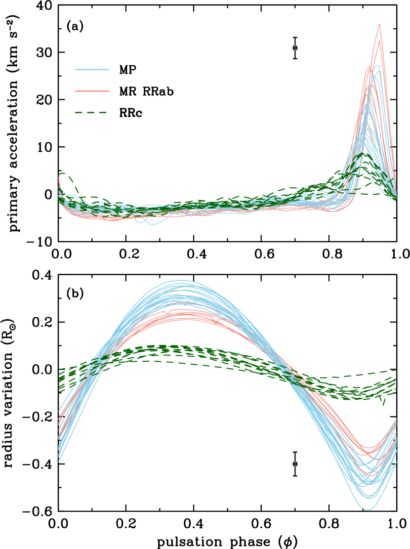
Figure 12: Dynamical acceleration and radius variation curves for individual RRc stars (green dashed lines), metal-rich RRab stars (MR; light red lines) and metal-poor RRab stars (MP; light blue lines).

The acceleration and the radius variation curves for individual RRc stars are shown in Figure 12. There is substantial star-to-star variation in acceleration maxima seen in panel (a), with AS211933 reaching $\sim$ 1.0 km s^-2 while AS143322 exhibits very little variation in its acceleration throughout its pulsational phases. In addition to the RRc curves we have added those for RRab stars from CSP17; see their Figure 11. Maxima of the RRc acceleration curves are about half those of metal-poor RRab and about one third of those of metal-rich RRab. The peak acceleration (the dynamical gravity) occurs near phase $\phi$ = 0.90 $\pm$ 0.05, during the phase of minimum radius displayed in panel (b) of Figure 12.

The data of Figure 12 show that the radius variations and primary accelerations of all RRc stars are markedly smaller than those of metal-rich (MR) and metal-poor (MP) RRab stars. In particular, the amplitudes of radius variations and the dynamical gravities of MP RRc stars are four times smaller than those of MP RRab stars. The time-average radii of RRc stars and those of MP and MR RRab stars occur at the same phases, $\phi$ = 0.65 $\pm$ 0.05 during infall and $\phi$ = 0.12 $\pm$ 0.05 during outflow. All RRc stars of this study, except AS143322 which exhibits the lowest dynamical gravity, possess more or less prominent H$\alpha$ radial velocity maxima or at least stationary values near phase $\phi$ = 0.52 $\pm$ 0.05 (Figures 10 and 11). This phenomenon, not seen in the metallic velocities, is restricted to the high atmosphere layers which produce Doppler cores of H$\alpha$.

7.2 Shock Waves

The primary accelerations are due to the behaviors of radiative opacities, the $\kappa$ and $\gamma$ mechanisms, that operate in the He⁺ and He⁺⁺ ionization zones that drive the pulsational instability. These processes create compression waves and under certain conditions shock waves, $Sh_{H+He}$, that move outward through mass shells. We have not detected any doubling of $H\alpha$ absorption lines or any H$\alpha$ emission during the primary accelerations of our RRc stars: shocks are weak or absent in the shallow RRc atmospheres. Failure to detect broadening of H$\alpha$ near phases of peak acceleration in our spectra sets an upper limit of approximately 10 km s^-1 on any shock discontinuities that might be present. We suppose instead that the prominent secondary radial velocity maxima or elbows near phase $\phi$ = 0.52 $\pm$ 0.05 in Figures 10 and 11, are caused by compression waves. These waves are qualitatively similar to $Sh_{PM3}$ in RRab stars described in Chadid et al. (2014), the cooling shock (Hill, 1972) that produces compression heating during infall. Such shocks are significant in extended atmospheres, leading to the prominent secondary maxima seen at H$\alpha$ $RV$ curves of metal-poor RRab stars.

7.3 Comparison of RRc Atmospheric Structures with those of RRab Stars

The linear regression of H$\alpha$ $RV$ amplitudes with those of metal lines in Figure 9 is highly determinate ($R^{2}$ = 0.98), it appears to be strictly linear in the interval 10 $<$ $\Delta RV_{m}$ $<$ 65 km s^-1, and it has a “non-physical y-intercept” of $-$14.5 km s^-1. The actual regression must become non-linear near the origin in a manner that permits both velocity amplitudes to approach zero together. This is a theoretical issue beyond the scope of our report.

Panel (a) of Figure 12 illustrates the small dynamical gravities of RRc overtone pulsators. As noted in §7.2 RRc stars may well be shock-free. The data panel (a) of this figure suggests a dynamical gravity division between the RRc and RRab stars near $d^{2}R/dt^{2}$ = 15 km s^-2. Photospheric radius variations of RRc are similarly smaller than those of RRab stars (panel (b) of Figure 12). The RRc radius variation average is approximately $R$ $\simeq$ 0.19 $R_{\odot}$.

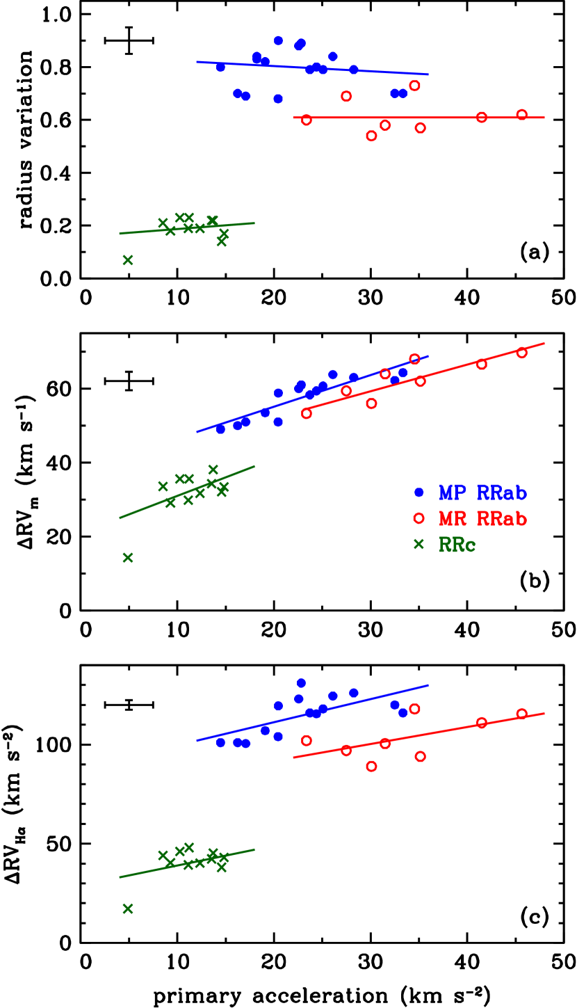
Figure 13: Radius variation, metal $RV$ amplitude and H$\alpha$ $RV$ amplitude $versus$ primary acceleration for RRc (green), metal-poor (blue) and metal-rich (red) RRab stars.

Figure 13 deserves some comment. Dynamical gravity, used as an independent variable, produces simple linear regressions for the radius variation, as well as the H$\alpha$ and metal line $RV$ amplitudes. We include the RRab data in CSP17 in all three panels of Figure 13 to show that the RRab and RRc stars lie on distinctly different regressions, i.e., motions of the upper-atmospheric and near-photospheric regions of RRc and RRab stars are distinctly different. Such differences in the atmospheric dynamics and structure are induced by large differences in the mechanical energy of the ballistic motion and the strengths of shock waves in their atmosphere. The RRc stars are trans-sonic regime stars (as characterized by CSP17); their pulsation excitation processes create atmospheric dynamics and structure that differ from those of the RRab stars.

8 TEST OF THE BLAZHKO ROTATOR HYPOTHESIS

Observed spectral line broadening is a convolution of axial rotation, macroturbulence, microturbulence, thermal effects, and spectrograph slit functions. The last three of these causes can be estimated and subtracted from the total, leaving a combination of macroturbulent and rotational line profiles. Preston & Chadid (2013) describe in detail these calculations, calling the result $V_{macrot}$. It is difficult to estimate the macroturbulence and rotation contributions to $V_{macrot}$ unless one or the other of them dominates the broadening. Here we attempt to detect rotational signatures in the line profiles of Blazhko RRc stars.

The majority of Blazhko periods exceed 12 days, and in these cases any line broadening produced by rotation would be unobservably small. To make our test we selected seven ASAS RRc stars for which the Szczygieł & Fabrycky (2007) Blazhko periods ($<$12 days) would produce axial equatorial rotational velocities $>$20 km s^-1, a value that we could measure from line profiles produced by the duPont echelle. To estimate these hypothetical axial rotations we adopted a mean radius $R_{RRc}/R_{\odot}$ = 4.56$\pm$0.42, which is the average of values obtained for two field RRc stars by use of the Baade-Wesselink method (Liu & Janes, 1990) and values obtained from Fourier decomposition of photometry of two RRc stars in the globular cluster M2 (Lázaro et al., 2006). Then, from $2\pi R$ = $V_{rot}P$ we obtain $V_{rot}$ (km s^-1) = 50.6($R_{RRc}/R_{\odot}$)/$P$(d), which yields the $V_{rot}$ values in column 3 of Table 12.

Then following the procedures of Preston & Chadid (2013) we have computed $V_{macrot}$ values from the observed line profiles for the seven chosen RRc stars, listing them in column 4 of Table 12. These are upper limits to the rotational broadening: $V_{rot}$sin($i$) $<$ $V_{macrot}$. Thus, upper limits to sin($i$) can be computed (column 5 of Table 12), translating to upper limits on axial inclinations $i$ (column 6). This distribution of maximum inclinations is improbable: if Blazhko periods were truly periods of axial rotation, we would have to be viewing Blazhko stars preferentially pole-on. We regard the improbability of this circumstance as falsification of the rotator hypothesis. We defer further discussion of this result to our next paper (Preston et al., 2017).

Figure 3: An example of co-addition of spectra, using the very metal-poor star AS162158. The chosen spectral region is rich in the lines of iron-group ions, and contains the well-known resonance line of Ba ii at 4554 Å. The top spectrum is one of the individual observed spectra obtained at pulsational phase $\phi$ $\simeq$ 0.35. The middle spectrum is the co-addition of three spectra near this phase; this spectrum was used in the phase-based atmospheric analysis for AS162158. The bottom spectrum is the mean spectrum of all 21 spectra gathered for this star. Phase information has been sacrificed to substantially increase the $S/N$ of this co-added spectrum.

Figure 4: Correlations of excitation potentials $\chi$ with derived line abundances of Fe i (filled circles) and Fe ii (open circles) line abundances in AS162158. Panel (a) has the abundances from the co-addition of three spectra at phase $\langle\phi\rangle$ = 0.632 are shown, and panel (b) has the abundances from co-addition of all 21 AS162158. The dotted lines in each panel represent the mean abundance of Fe from the species abundances in that panel.

Figure 5: Panel (a): Comparison of metallicity values computed by forming for each star the mean of values derived at the co-added phase points (labeled $\langle$[Fe/H]$\rangle$ $-$ all phases), and the value derived from the total spectrum formed from the addition of all individual spectra regardless of their phases (called [Fe/H] $-$ mean spectrum). The dotted line shows equality of the metallicities, and the dashed line shows the derived mean offset in these values. Panel (b): Differences between the relative abundance ratios [Ti/Fe] between those determined from the total spectra and those determined from the averages of individual phases. An example of co-addition of spectra, using the very metal-poor star AS162158. The dotted line represents equality of the two [Ti/Fe] values, and the dashed line represents the derived mean offset from equality.

Figure 8: Visual light amplitude versus $RV$ amplitude. The blue solid circles (MP RRab stars) and green crosses (MP RRc stars) denote field RR Lyrae stars of this study. Black points are RRab and RRc stars in globular cluster M3 ([Fe/H] $\simeq$ $-$1.5) studied by Jurcsik et al. (2015, 2017). The dashed regression line is for the RRc field stars, the dotted line is for the RRab field stars, and the solid line is for the M3 RRab stars. The field MR RRab stars are not shown in this figure.

Table 1: Program Star Data

ASAS Name	Other Name	[Fe/H]	$P$	$HJD_{0}$	$V_{min}$	$V_{amp}$	$RV_{amp}$
			ASAS	this study	ASAS	ASAS	this study
Stable RRc Stars
014500-3003.6	SC Sci	$-$2.28	0.377380	1869.075	11.14	0.52	$\cdots$
023706-4257.8	CS Eri	$-$1.88	0.311326	1868.717	8.84	0.50	29.0
094541-0644.0	RU Sex	$-$2.10	0.350225	1869.604	10.60	0.44	27.5
095328+0203.5	T Sex	$-$1.76	0.324697	1869.758	9.85	0.43	$\cdots$
101332-0702.3		$-$1.73	0.313619	1869.690	10.78	0.40	$\cdots$
123811-1500.0	Y Crv	$-$1.39	0.329045	1884.258	11.42	0.44	25.6
132225-2042.3	BD-19 3673	$-$0.96	0.235934	1888.536	10.72	0.40	25.0
132448-0658.8	AU Vir	$-$2.04	0.323237	1900.042	11.43	0.51	27.5
143322-0418.2	BD-03 3640	$-$1.48	0.249632	1907.348	10.61	0.23	12.0
190212-4639.2	MT Tel	$-$2.58	0.316690	1954.795	8.75	0.55	21.4
203145-2158.7		$-$1.17	0.310712	1873.190	11.27	0.38	$\cdots$
211933-1507.0	YZ Cap	$-$1.50	0.273460	1873.307	11.11	0.50	25.6
Blazhko RRc Stars
081933-2358.2	V701 Pup	$-$2.50	0.285667	4900.180	10.42	0.28	$\cdots$
085254-0300.3		$-$1.50	0.266902	4900.400	12.46	0.47	$\cdots$
090900-0410.4		$-$1.98	0.303261	4900.200	10.69	0.41	$\cdots$
110522-2641.0		$-$1.60	0.294510	4900.150	11.66	0.39	$\cdots$
162158+0244.5		$-$1.83	0.323698	4900.435	12.62	0.40	$\cdots$
200431-5352.3		$-$2.66	0.300240	4900.470	11.01	0.28	$\cdots$
230659-4354.6	BO Gru	$-$1.24	0.281130	5014.925	12.79	0.30	$\cdots$

Table 2: Radial Velocities

Star	file	HJD	$\phi$	RV(metals)	RV(H$\alpha$)
		d		km s-1	km s-1
AS014500	ccd6630	6916.7317	0.059	$-$29.1	$-$43.6
AS014500	ccd6631	6916.7370	0.074	$-$29.5	$-$43.0
AS014500	ccd6632	6916.7424	0.088	$-$27.9	$-$42.4
AS014500	ccd6633	6916.7477	0.102	$-$27.2	$-$43.1
AS014500	ccd6634	6916.7531	0.116	$-$26.7	$-$44.6
AS014500	ccd6635	6916.7584	0.130	$-$25.5	$-$42.3
AS014500	ccd6637	6916.7659	0.150	$-$25.9	$-$42.6
AS014500	ccd6638	6916.7712	0.164	$-$24.1	$-$38.8
AS014500	ccd6639	6916.7765	0.178	$-$23.2	$-$39.0
AS014500	ccd6640	6916.7819	0.192	$-$22.4	$-$36.9

(This table is available in its entirety in machine-readable form.)

Table 3: Phases of Radial Velocity and Photometric Minimas

Star	$\phi_{min}$	$\phi_{min}$	$\Delta\phi$	source
	$RV$	$V_{mag}$
RRab Stars
TW Her	1.010	1.005	0.005	1
UU Vir	1.030	1.000	0.030	1
V445 Oph	1.000	1.000	0.000	2
SS Leo	1.020	1.000	0.020	2
WY Ant	0.990	1.000	$-$0.010	3
W Crt	1.010	1.000	0.010	3
BB Pup	1.025	1.000	0.025	3
SW And	1.040	1.000	0.040	4
SW Dra	1.025	1.000	0.025	4
SS For	1.020	1.005	0.015	4
RV Phe	1.010	1.005	0.005	4
V440 Sgr	1.000	1.010	$-$0.010	4
SW And	1.020	1.005	0.015	5
RR Cet	1.015	0.985	0.030	5
SU Dra	1.000	0.995	0.005	5
RX Eri	1.000	1.000	0.000	5
TT Lyn	1.000	1.000	0.000	5
AV Peg	1.000	1.000	0.000	5
AR Per	1.005	1.000	0.005	5
TU UMa	1.020	0.995	0.025	5
mean			0.012
$\sigma$			0.014
RRc Stars
DH Peg	1.045	0.995	0.050	6
T Sex	1.000	0.990	0.010	5
v056	0.000	-0.005	0.005	7
v086	0.005	0.000	0.005	7
v097	$-$0.010	-0.020	0.010	7
v107	0.040	0.010	0.030	7
mean			0.018
$\sigma$			0.014

References. — 1 - Jones et al. (1988b); 2 - Fernley et al. (1990); 3 - Skillen et al. (1993); 4 - Cacciari et al. (1987); 5 - Liu & Janes (1989); 6 - Jones et al. (1988a): 7 - Jurcsik et al. (2015, 2017)

Table 4: Stellar Parameters from Phased-Averaged Spectra

Star	$\phi$	num	Teff	log g	[M/H]	$\xi_{\rm t}$	[Fe/H]	$\sigma$	#	[Fe/H]	$\sigma$	#
			K			km s-1	I	I	I	II	II	II
AS014500	0.055	6	7650	3.70	-2.00	3.0	-1.98	0.29	16	-1.94	0.22	11
AS014500	0.146	6	7500	3.50	-2.00	3.0	-1.95	0.12	24	-1.95	0.26	14
AS014500	0.247	7	7200	2.90	-2.00	2.5	-2.04	0.20	26	-2.01	0.22	19
AS014500	0.353	7	6700	2.80	-2.00	2.5	-2.09	0.29	34	-2.05	0.24	22
AS014500	0.451	6	6950	3.00	-2.00	3.2	-2.09	0.22	26	-2.12	0.26	17
AS014500	0.566	5	6950	3.00	-2.00	2.6	-1.98	0.25	24	-2.00	0.26	15
AS014500	0.661	5	7050	3.20	-2.00	2.5	-2.02	0.21	22	-1.99	0.20	13
AS014500	0.743	6	7650	3.50	-2.00	2.5	-1.99	0.18	15	-2.00	0.18	11
AS014500	0.834	6	7650	4.00	-2.00	2.5	-2.01	0.18	8	-1.97	0.26	5
AS023706	0.049	5	7150	2.10	1.90	2.3	-1.86	0.17	48	-1.86	0.14	33
AS023706	0.161	5	7000	2.10	-1.90	2.0	-1.82	0.14	61	-1.80	0.12	35
AS023706	0.255	5	6850	2.10	-1.90	2.3	-1.84	0.12	64	-1.82	0.13	38
AS023706	0.355	6	6650	2.10	-1.90	2.5	-1.85	0.13	74	-1.85	0.14	39
AS023706	0.461	5	6650	2.40	-1.90	2.4	-1.79	0.14	74	-1.79	0.15	35
AS023706	0.589	5	6650	2.40	-1.90	2.4	-1.83	0.14	64	-1.82	0.15	33
AS023706	0.747	6	7000	2.60	-1.80	2.6	-1.77	0.14	60	-1.79	0.12	35
AS023706	0.857	6	7300	2.60	1.80	2.0	-1.87	0.14	35	-1.88	0.18	27
AS023706	0.959	5	7300	2.60	-1.80	2.2	-1.89	0.16	39	-1.87	0.11	28

(This table is available in its entirety in machine-readable form.)

Table 5: Mean Stellar Parameters: Phased-Averaged Spectra

Star	$\phi$	num	Teff	log g	[M/H]	$\xi_{\rm t}$	[Fe/H]	$\sigma$	#	[Fe/H]	$\sigma$	#
			K			km s-1	I	I	I	II	II	II
AS014500	0.44	6	7256	3.29	-2.00	2.7	-2.02	0.05	22	-2.00	0.05	14
AS023706	0.50	5	6950	2.33	-1.04	2.3	-1.84	0.04	58	-1.83	0.03	34
AS081933	0.59	3	7400	3.70	-2.35	1.8	-2.50	0.03	12	-2.53	0.01	9
AS085254	0.61	2	7267	2.63	-1.53	2.9	-1.60	0.05	24	-1.61	0.07	20
AS090900	0.14	3	7300	2.50	-1.80	2.9	-1.93	0.05	18	-1.95	0.04	13
AS094541	0.42	8	6963	2.60	-2.00	2.5	-1.98	0.04	27	-1.98	0.04	18
AS095328	0.35	8	6958	2.12	-1.48	2.3	-1.48	0.10	61	-1.49	0.11	34
AS101332	0.39	9	6736	2.19	-1.50	3.1	-1.48	0.07	54	-1.47	0.08	31
AS110522	0.55	3	7175	2.88	-1.68	2.1	-1.73	0.16	23	-1.73	0.17	17
AS123811	0.49	7	7360	2.90	-1.23	3.0	-1.21	0.09	34	-1.22	0.08	24
AS132225	0.44	6	6979	2.27	-0.71	3.0	-0.96	0.04	56	-0.96	0.03	30
AS132448	0.50	6	7050	2.50	-1.98	2.4	-1.92	0.24	15	-1.93	0.25	9
AS143322	0.46	6	7311	2.77	-1.29	3.0	-1.26	0.12	99	-1.25	0.12	34
AS162158	0.35	4	7408	3.48	-1.53	2.8	-1.56	0.11	13	-1.58	0.08	11
AS190212	0.48	6	7270	3.23	-2.71	2.1	-2.70	0.16	20	-2.71	0.17	13
AS200431	0.47	4	7486	3.37	-1.86	2.0	-2.42	0.19	10	-2.40	0.18	7
AS203145	0.44	5	6663	2.20	-0.59	3.3	-1.09	0.06	66	-1.07	0.05	30
AS211933	0.52	5	7044	2.15	-1.46	2.5	-1.49	0.05	66	-1.46	0.06	30
AS230659	0.45	5	7550	2.93	-1.48	2.8	-1.58	0.07	15	-1.56	0.12	13

Table 6: Mean Stellar Parameters: Total Spectra

Star	$\phi$	num	Teff	log g	[M/H]	$\xi_{\rm t}$	[Fe/H]	$\sigma$	#	[Fe/H]	$\sigma$	#
			K			km s-1	I	I	I	II	II	II
AS014500	all	54	6950	2.50	$-$2.00	2.2	$-$2.30	0.19	34	$-$2.26	0.19	23
AS023706	all	48	6850	2.20	$-$1.90	2.1	$-$1.90	0.12	63	$-$1.87	0.13	35
AS081933	all	6	7550	3.00	$-$2.50	1.0	$-$2.48	0.14	15	$-$2.52	0.15	12
AS085254	all	6	7400	2.80	$-$1.50	2.2	$-$1.49	0.19	31	$-$1.51	0.22	26
AS090900	all	6	7150	2.40	$-$1.90	2.5	$-$1.98	0.20	18	$-$1.97	0.15	17
AS094541	all	67	6900	2.60	$-$2.00	2.0	$-$2.11	0.17	36	$-$2.10	0.15	20
AS095328	all	50	7000	2.30	$-$1.40	1.2	$-$1.76	0.14	57	$-$1.76	0.15	35
AS101332	all	62	6600	2.10	$-$1.60	2.0	$-$1.74	0.18	62	$-$1.72	0.17	36
AS110522	all	18	7500	3.20	$-$1.60	1.5	$-$1.61	0.20	32	$-$1.58	0.14	25
AS123811	all	65	7200	2.70	$-$1.40	2.5	$-$1.41	0.23	57	$-$1.37	0.19	35
AS132225	all	39	7100	2.40	$-$1.00	2.0	$-$0.98	0.16	77	$-$0.95	0.16	39
AS132448	all	58	7100	2.70	$-$2.00	1.5	$-$2.04	0.20	27	$-$2.03	0.23	24
AS143322	all	53	7100	2.30	$-$1.40	2.0	$-$1.47	0.13	65	$-$1.48	0.12	32
AS162158	all	21	7600	3.20	$-$1.80	2.5	$-$1.83	0.19	22	$-$1.83	0.15	17
AS190212	all	59	7500	3.70	$-$2.60	1.7	$-$2.59	0.05	20	$-$2.56	0.10	14
AS200431	all	29	7600	3.20	$-$2.60	3.0	$-$2.67	0.14	14	$-$2.65	0.21	13
AS203145	all	38	6600	1.90	$-$1.10	3.0	$-$1.18	0.18	77	$-$1.16	0.17	37
AS211933	all	43	7200	2.20	$-$1.50	2.3	$-$1.51	0.13	58	$-$1.50	0.15	37
AS230659	all	28	7750	3.10	$-$1.40	1.2	$-$1.26	0.25	33	$-$1.23	0.22	25

Table 7: Relative Abundances of $\alpha$ Elements

Star	[Mg/Fe]	$\sigma$	#	[Si/Fe]	$\sigma$	#	[Si/Fe]	$\sigma$	#	[Ca/Fe]	$\sigma$	#	[Ti/Fe]	$\sigma$	#	[Ti/Fe]	$\sigma$	#
	I	I	I	I	I	I	II	II	II	I	I	I	I	I	I	II	II	II
AS014500	0.46	0.25	3	0.05	$\cdots$	1	0.47	0.03	3	0.48	0.27	7	$\cdots$	$\cdots$	$\cdots$	0.44	0.12	15
AS023706	0.43	0.30	4	-0.17	$\cdots$	1	0.30	0.09	3	0.34	0.14	12	0.26	0.11	4	0.46	0.36	19
AS081933	0.44	0.12	4	-0.03	$\cdots$	1	0.89	0.36	2	0.28	0.30	2	$\cdots$	$\cdots$	$\cdots$	0.62	0.12	10
AS085254	0.67	0.27	4	0.41	$\cdots$	1	0.26	0.11	3	0.30	0.41	4	0.12	$\cdots$	1	0.51	0.27	15
AS090900	0.17	0.37	3	0.52	$\cdots$	1	0.53	0.39	2	0.44	0.23	2	$\cdots$	$\cdots$	$\cdots$	0.37	0.18	13
AS094541	0.64	0.36	4	0.48	$\cdots$	1	0.59	$\cdots$	1	0.37	0.21	7	0.60	0.13	2	0.63	0.22	13
AS095328	0.51	0.18	3	0.09	$\cdots$	1	0.51	0.01	2	0.40	0.16	8	0.33	0.14	3	0.50	0.31	17
AS101332	0.25	0.38	3	0.31	$\cdots$	1	0.71	0.35	2	0.36	0.14	11	0.21	0.22	4	0.42	0.17	15
AS110522	0.49	0.17	3	0.29	$\cdots$	1	0.19	0.04	2	0.60	0.41	2	$\cdots$	$\cdots$	$\cdots$	0.62	0.29	14
AS123811	0.61	0.28	3	0.36	$\cdots$	1	0.25	0.24	3	0.32	0.15	11	0.41	0.20	7	0.42	0.17	16
AS132225	0.38	0.09	3	0.11	$\cdots$	1	0.29	0.13	3	0.10	0.16	13	0.20	0.19	3	0.19	0.23	13
AS132448	0.81	0.30	3	0.84	$\cdots$	1	0.40	0.14	2	0.52	0.39	4	$\cdots$	$\cdots$	$\cdots$	0.67	0.38	14
AS143322	0.52	$\cdots$	1	0.50	$\cdots$	1	0.51	0.20	3	0.35	0.19	9	0.27	0.19	3	0.36	0.18	12
AS162158	0.11	0.26	3	0.02	$\cdots$	1	$\cdots$	$\cdots$	$\cdots$	-0.06	$\cdots$	1	$\cdots$	$\cdots$	$\cdots$	0.47	0.13	9
AS190212	0.27	0.20	4	-0.01	$\cdots$	1	0.50	0.12	2	0.26	0.07	2	$\cdots$	$\cdots$	$\cdots$	0.60	0.16	13
AS200431	0.06	0.12	3	-0.06	$\cdots$	1	0.32	$\cdots$	1	$\cdots$	$\cdots$	$\cdots$	$\cdots$	$\cdots$	$\cdots$	0.56	0.12	12
AS203145	0.33	0.23	3	0.63	$\cdots$	1	0.65	0.11	2	0.32	0.17	14	0.28	0.11	5	0.28	0.20	15
AS211933	0.70	0.18	3	0.20	$\cdots$	1	0.48	0.15	3	0.39	0.15	11	0.38	0.04	3	0.50	0.36	15
AS230659	0.38	$\cdots$	1	0.35	$\cdots$	1	0.25	0.30	2	0.08	0.35	6	0.28	0.23	2	0.26	0.17	7
mean	0.43			0.26			0.45			0.33			0.30			0.47
$\pm$	0.05			0.06			0.05			0.04			0.04			0.03
num	18			18			17			17			10			18
$\sigma$(mean)	0.21			0.27			0.19			0.16			0.13			0.13

Table 8: Relative Abundances of Fe-group and $n$-capture Elements

Star	[Sc/Fe]	$\sigma$	#	[Cr/Fe]	$\sigma$	#	[Cr/Fe]	$\sigma$	#	[Zn/Fe]	$\sigma$	#	[Sr/Fe]	$\sigma$	#	[Ba/Fe]	$\sigma$	#
	II	II	II	I	I	I	II	II	II	I	I	I	II	II	II	II	II	II
AS014500	0.03	0.14	4	$-$0.07	0.14	3	0.14	0.16	4	$\cdots$	$\cdots$	$\cdots$	0.24	0.06	2	0.12	0.02	2
AS023706	$-$0.13	0.10	5	$-$0.04	0.11	4	$-$0.07	0.16	4	0.12	$\cdots$	1	0.40	$\cdots$	1	$-$0.03	0.14	3
AS081933	0.40	0.26	4	$-$0.08	$\cdots$	1	0.07	$\cdots$	1	$\cdots$	$\cdots$	$\cdots$	0.06	0.19	2	$\cdots$	$\cdots$	$\cdots$
AS085254	0.17	0.22	5	$-$0.10	0.21	3	0.01	0.09	4	0.25	$\cdots$	1	0.10	$\cdots$	1	0.56	0.90	2
AS090900	$-$0.06	0.29	3	0.10	0.05	3	$\cdots$	$\cdots$	$\cdots$	$\cdots$	$\cdots$	$\cdots$	$-$0.17	0.01	2	0.19	0.17	3
AS094541	0.17	0.06	4	$\cdots$	$\cdots$	$\cdots$	0.11	0.10	3	$\cdots$	$\cdots$	$\cdots$	$\cdots$	$\cdots$	$\cdots$	0.13	0.02	2
AS095328	0.13	0.26	4	$-$0.18	0.12	4	$-$0.08	0.04	4	0.30	0.01	2	0.70	0.00	2	0.16	0.10	3
AS101332	$-$0.12	0.18	3	$-$0.03	0.12	5	$-$0.09	0.06	3	0.33	0.14	2	$\cdots$	$\cdots$	$\cdots$	0.30	0.21	3
AS110522	0.43	0.27	4	$-$0.04	0.18	4	0.15	0.16	3	$\cdots$	$\cdots$	$\cdots$	$-$0.03	0.40	2	$-$0.24	0.05	2
AS123811	$-$0.03	0.13	5	$-$0.19	0.12	4	$-$0.06	0.13	4	0.56	$\cdots$	1	$\cdots$	$\cdots$	$\cdots$	$-$0.01	0.29	3
AS132225	$-$0.27	0.13	4	$-$0.07	0.22	4	$-$0.01	0.10	4	0.30	$\cdots$	1	$\cdots$	$\cdots$	$\cdots$	$-$0.50	0.31	3
AS132448	0.32	0.20	4	$-$0.16	0.07	3	0.05	0.10	2	$\cdots$	$\cdots$	$\cdots$	0.12	0.11	2	$-$0.32	0.12	2
AS143322	$-$0.02	0.21	4	$-$0.08	0.11	4	$-$0.08	0.06	3	0.32	0.20	2	$\cdots$	$\cdots$	$\cdots$	$-$0.16	0.11	2
AS162158	0.19	0.24	3	$-$0.11	0.16	2	0.11	0.04	2	$\cdots$	$\cdots$	$\cdots$	$-$0.17	$\cdots$	1	0.23	0.15	2
AS190212	0.30	0.05	2	0.00	0.03	3	0.27	0.04	2	$\cdots$	$\cdots$	$\cdots$	$-$0.31	0.01	2	$\cdots$	$\cdots$	$\cdots$
AS200431	0.36	0.19	2	0.17	0.14	2	0.23	0.07	2	$\cdots$	$\cdots$	$\cdots$	$-$0.81	0.08	2	$\cdots$	$\cdots$	$\cdots$
AS203145	$-$0.68	0.12	4	$-$0.09	0.26	5	0.06	0.22	4	0.32	0.02	2	$\cdots$	$\cdots$	$\cdots$	$-$0.43	0.04	3
AS211933	$-$0.03	0.29	4	$-$0.10	0.10	4	$-$0.01	0.08	4	0.25	0.05	2	$\cdots$	$\cdots$	$\cdots$	$-$0.27	0.03	2
AS230659	0.04	0.60	5	$-$0.11	0.18	3	0.09	0.14	4	$\cdots$	$\cdots$	$\cdots$	1.13	0.22	2	0.64	$\cdots$	1
mean	0.06			$-$0.07			0.05			0.30			0.11			0.02
$\pm$	0.06			0.02			0.03			0.04			0.15			0.09
num	18			17			17			9			11			15
$\sigma$(mean)	0.27			0.09			0.11			0.11			0.50			0.33

Table 9: Radial Velocity Shift and Stretch Parameters

Star	Shift	$\Delta$RV=24	$\Delta$RV=30
	km s-1	km s-1	km s-1
AS023706	151.0	0.816	1.02
AS094541	$-$200.0	0.864	1.08
AS123811	$-$147.0	0.938	1.17
AS132225	5.4	0.944	1.18
AS132448	$-$104.5	0.912	1.14
AS190212	$-$87.2	1.112	1.39
AS211933	133.3	0.944	1.18
mean		0.933	1.17
$\sigma$		0.092	0.12

Table 10: Mean Velocity Curve Templates

$\phi$	$\Delta$RV(s1,s2)	$\Delta$RV(s1,s2)	$\phi$	$\Delta$RV(s1,s2)
	$\Delta$RV=30	$\Delta$RV=24		$\Delta$RV=40
	km s-1	km s-1		km s-1
0.00	$-$17.5	$-$14.0	0.013	$-$18.6
0.02	$-$17.2	$-$13.8	0.047	$-$23.1
0.04	$-$16.5	$-$13.2	0.080	$-$24.6
0.06	$-$15.7	$-$12.6	0.113	$-$22.3
0.08	$-$14.8	$-$11.8	0.147	$-$19.8
0.10	$-$13.9	$-$11.1	0.180	$-$17.1
0.12	$-$12.8	$-$10.2	0.213	$-$13.9
0.14	$-$11.7	$-$9.4	0.246	$-$10.5
0.16	$-$10.4	$-$8.3	0.280	$-$7.2
0.18	$-$9.0	$-$7.2	0.313	$-$4.0
0.20	$-$7.5	$-$6.0	0.346	$-$0.9
0.22	$-$6.0	$-$4.8	0.380	2.4
0.24	$-$4.4	$-$3.5	0.413	5.9
0.26	$-$3.0	$-$2.4	0.446	9.1
0.28	$-$1.7	$-$1.4	0.480	11.4
0.30	$-$0.5	$-$0.4	0.513	13.2
0.32	0.6	0.5	0.546	13.8
0.34	1.4	1.1	0.579	13.7
0.36	2.2	1.8	0.613	13.4
0.38	3.1	2.5	0.646	13.0
0.40	3.9	3.1	0.679	13.2
0.42	4.8	3.8	0.713	14.0
0.44	5.5	4.4	0.746	14.6
0.46	6.5	5.2	0.779	15.4
0.48	7.2	5.8	0.813	14.4
0.50	7.9	6.3	0.846	11.2
0.52	8.7	7.0	0.879	4.4
0.54	9.4	7.5	0.912	$-$2.6
0.56	10.1	8.1	0.946	$-$7.1
0.58	10.7	8.6	0.979	$-$12.6
0.60	11.2	9.0	1.012	$-$18.6
0.62	11.7	9.4
0.64	11.9	9.5
0.66	12.0	9.6
0.68	12.1	9.7
0.70	12.1	9.7
0.72	11.8	9.4
0.74	11.4	9.1
0.76	10.4	8.3
0.78	9.4	7.5
0.80	8.2	6.6
0.82	6.9	5.5
0.84	5.2	4.2
0.86	3.3	2.6
0.88	0.3	0.2
0.90	$-$4.0	$-$3.2
0.92	$-$8.5	$-$6.8
0.94	$-$12.5	$-$10.0
0.96	$-$15.8	$-$12.6
0.98	$-$17.3	$-$13.8

Table 11: Motion Parameters for Selected RRc Program Stars

Star	Primary	Radius	Metal RV	H$\alpha$ RV	$\gamma$–velocity
	acceleration	variation	amplitude	amplitude
	km s-2	R⊙	km s-1	km s-1	km s-1
AS014500	8.51	0.21	33.60	44.10	$-$17
AS023706	13.71	0.22	38.08	45.34	$-$148
AS094541	10.28	0.23	35.61	46.12	184
AS101332	12.33	0.19	31.74	40.26	215
AS123811	13.53	0.22	34.30	42.32	126
AS132225	14.59	0.14	32.09	38.10	91
AS132448	11.22	0.23	35.64	48.02	91
AS143322	4.88	0.07	14.32	17.21	$-$65
AS190212	9.29	0.18	29.13	40.36	62
AS203145	11.15	0.19	29.87	39.31	$-$5
AS211933	14.83	0.17	33.42	43.04	$-$112

Table 12: Rotation Parameters for Blazhko Stars

Star	PBlazhko	$V_{rot}$	$V_{macrot}$	sin($i$)	$i$
	days	km s-1	km s-1		deg
AS081933	8.1	28	5.8	$<$0.204	$<$11.8
AS085254	11.8	20	6.1	$<$0.313	$<$18.2
AS090900	8.5	27	14.4	$<$0.533	$<$32.2
AS110522	7.4	31	9.6	$<$0.309	$<$18.0
AS162158	8.1	28	12.2	$<$0.430	$<$25.5
AS200431	10.8	21	7.6	$<$0.357	$<$20.9
AS230659	10.2	22	12.0	$<$0.534	$<$32.3

References

- Asplund et al. (2009) Asplund, M., Grevesse, N., Sauval, A. J., & Scott, P. 2009, ARA&A, 47, 481
- Blažko (1907) Blažko, S. 1907, Astronomische Nachrichten, 175, 325
- Bono et al. (1994) Bono, G., Caputo, F., & Stellingwerf, R. F. 1994, ApJ, 432, L51
- Burki et al. (1982) Burki, G., Mayor, M., & Benz, W. 1982, A&A, 109, 258
- Cacciari et al. (1987) Cacciari, C., Clementini, G., Prevot, L., et al. 1987, A&AS, 69, 135
- Chadid & Preston (2013) Chadid, M., & Preston, G. W. 2013, MNRAS, 434, 552
- Chadid et al. (2017) Chadid, M., Sneden, C., & Preston, G. W. 2017, ApJ, 835, 187
- Chadid et al. (2014) Chadid, M., Vernin, J., Preston, G., et al. 2014, AJ, 148, 88
- Drake et al. (2014) Drake, A. J., Graham, M. J., Djorgovski, S. G., et al. 2014, ApJS, 213, 9
- Fernley & Barnes (1997) Fernley, J., & Barnes, T. G. 1997, A&AS, 125, doi:10.1051/aas:1997222
- Fernley et al. (1998) Fernley, J., Barnes, T. G., Skillen, I., et al. 1998, A&A, 330, 515
- Fernley et al. (1990) Fernley, J. A., Skillen, I., Jameson, R. F., & Longmore, A. J. 1990, MNRAS, 242, 685
- For et al. (2011a) For, B.-Q., Preston, G. W., & Sneden, C. 2011a, ApJS, 194, 38
- For et al. (2011b) For, B.-Q., Sneden, C., & Preston, G. W. 2011b, ApJS, 197, 29
- Govea et al. (2014) Govea, J., Gomez, T., Preston, G. W., & Sneden, C. 2014, ApJ, 782, 59
- Hawley et al. (1986) Hawley, S. L., Jefferys, W. H., Barnes, III, T. G., & Lai, W. 1986, ApJ, 302, 626
- Hill (1972) Hill, S. J. 1972, ApJ, 178, 793
- Jones et al. (1988a) Jones, R. V., Carney, B. W., & Latham, D. W. 1988a, ApJ, 326, 312
- Jones et al. (1988b) —. 1988b, ApJ, 332, 206
- Jurcsik et al. (2015) Jurcsik, J., Smitola, P., Hajdu, G., et al. 2015, ApJS, 219, 25
- Jurcsik et al. (2017) —. 2017, MNRAS, 468, 1317
- Kollmeier et al. (2013) Kollmeier, J. A., Szczygieł, D. M., Burns, C. R., et al. 2013, ApJ, 775, 57
- Kurucz (2011) Kurucz, R. L. 2011, Canadian Journal of Physics, 89, 417
- Layden (1994) Layden, A. C. 1994, AJ, 108, 1016
- Lázaro et al. (2006) Lázaro, C., Arellano Ferro, A., Arévalo, M. J., et al. 2006, MNRAS, 372, 69
- Liu (1991) Liu, T. 1991, PASP, 103, 205
- Liu & Janes (1989) Liu, T., & Janes, K. A. 1989, ApJS, 69, 593
- Liu & Janes (1990) —. 1990, ApJ, 354, 273
- Mateu et al. (2012) Mateu, C., Vivas, A. K., Downes, J. J., et al. 2012, MNRAS, 427, 3374
- Neilson et al. (2012) Neilson, H. R., Nardetto, N., Ngeow, C.-C., Fouqué, P., & Storm, J. 2012, A&A, 541, A134
- Nemec et al. (2017) Nemec, J. M., Balona, L. A., Murphy, S. J., Kinemuchi, K., & Jeon, Y.-B. 2017, MNRAS, 466, 1290
- Nemec et al. (1995) Nemec, J. M., Mateo, M., Burke, M., & Olszewski, E. W. 1995, AJ, 110, 1186
- Ngeow et al. (2012) Ngeow, C.-C., Neilson, H. R., Nardetto, N., & Marengo, M. 2012, A&A, 543, A55
- Pietrzyński et al. (2012) Pietrzyński, G., Thompson, I. B., Gieren, W., et al. 2012, Nature, 484, 75
- Pojmański (2003) Pojmański, G. 2003, Acta Astron., 53, 341
- Pojmanski (2002) Pojmanski, G. 2002, Acta Astron., 52, 397
- Preston & Chadid (2013) Preston, G. W., & Chadid, M. 2013, in EAS Publications Series, Vol. 63, EAS Publications Series, ed. G. Alecian, Y. Lebreton, O. Richard, & G. Vauclair, 35–45
- Preston et al. (2017) Preston, G. W., Chadid, M., & Sneden, C. 2017, in preparation
- Preston & Landolt (1999) Preston, G. W., & Landolt, A. U. 1999, AJ, 118, 3006
- Preston & Sneden (2000) Preston, G. W., & Sneden, C. 2000, AJ, 120, 1014
- Przybylski (1983) Przybylski, A. 1983, Acta Astron., 33, 141
- Sanford (1930) Sanford, R. F. 1930, ApJ, 72, doi:10.1086/143259
- Sesar (2012) Sesar, B. 2012, AJ, 144, 114
- Skillen et al. (1993) Skillen, I., Fernley, J. A., Stobie, R. S., & Jameson, R. F. 1993, MNRAS, 265, 301
- Sneden (1973) Sneden, C. 1973, ApJ, 184, 839
- Sneden & Lawler (2008) Sneden, C., & Lawler, J. E. 2008, in American Institute of Physics Conference Series, Vol. 990, First Stars III, ed. B. W. O’Shea & A. Heger, 90–103
- Solano et al. (1997) Solano, E., Garrido, R., Fernley, J., & Barnes, T. G. 1997, A&AS, 125, doi:10.1051/aas:1997223
- Soszyński et al. (2014) Soszyński, I., Udalski, A., Szymański, M. K., et al. 2014, Acta Astron., 64, 177
- Strugnell et al. (1986) Strugnell, P., Reid, N., & Murray, C. A. 1986, MNRAS, 220, 413
- Szczygieł & Fabrycky (2007) Szczygieł, D. M., & Fabrycky, D. C. 2007, MNRAS, 377, 1263