RMPD – A Recursive Mid-Point Displacement Algorithm for Path Planning

Abstract

Motivated by what is required for real-time path planning, the paper starts out by presenting RMPD, a new recursive “local” planner founded on the key notion that, unless made necessary by an obstacle, there must be no deviation from the shortest path between any two points, which would normally be a straight line path in the configuration space. Subsequently, we increase the power of RMPD by introducing the notion of cost-awareness into the algorithm to improve the path quality – this is done by associating obstacle and smoothness costs with the currently selected path points and factoring those costs in choosing the best points for the next iteration. In this manner, the overall strategy in the cost-aware form of RMPD, cRMPD, combines the computational efficiency made possible by the recursive RMPD planner with the cost efficacy of a stochastic trajectory optimizer to rapidly produce high-quality local collision-free paths. Based on the test cases we have run, our experiments show that cRMPD can reduce planning time by up to two orders of magnitude as compared to RRT-Connect, while still maintaining a path length optimality equivalent to that of RRT*.

1 Introduction

Path planning has been an important area of research in robotics over the last several decades. Path planning algorithms have important uses in robotic assembly (?), autonomous driving (?), kinematic and dynamic control for robots, etc.

In traditional approaches to path planning, one first overlays a grid of points on the configuration space and then develops an obstacle-free path incrementally from the start configuration to the goal configuration, going from one grid point to the next in the process. Subsequently, a search is carried out over the paths thus discovered to find the optimal path that connects the goal configuration with the start configuration. These algorithms are known to work well in low-dimensional configuration spaces. However, as the dimensionality of the space increases, they extract a large performance penalty.

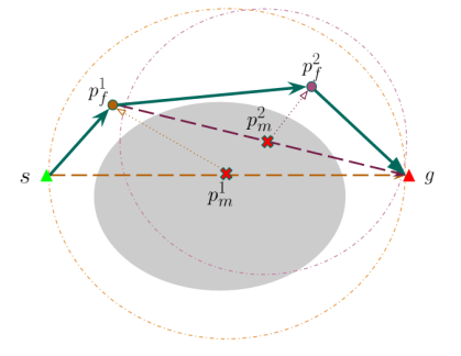
Figure 1: RMPD uses recursion to efficiently find a detour around an obstacle. Shown as $p_{m}^{1}$ and $p_{m}^{2}$ are the mid-points of two candidate path segments, each of which contains at least one in-collision point. The detouring collision-free replacements for the mid-points are shown as $p_{f}^{1}$ and $p_{f}^{2}$. The dashed circles represents the search hypersphere for middle point replacement.

More recently, sampling based algorithms have gained considerable prominence. The basic idea of such algorithms is to sample the configuration space at randomly selected points until a connection of the local pathways thus constructed can lead one from the start configuration to the goal configuration. These are best exemplified by the Probabilistic Roadmap Method (PRM) (?), the Randomized Potential Fields (?), and the Rapidly-exploring Random Tree (RRT) (?). The important factors that account for the popularity of such algorithms include : (1) They can be used with greater ease in high dimensional configuration spaces compared to the traditional algorithms; (2) The algorithms based on PRM and RRT can be shown to be probabilistically complete; (3) The ease in merging partially developed solutions in order to respond simultaneously to multiple path planning queries; etc.

In our laboratory we have been exploring the use of RRT and RRT-Connect (?) algorithms for real-time motion planning as needed for automatic pruning of dormant trees — a crucial step in growing healthy apple orchards. Our main concern has been the limited extent to which a straightforward application of RRT-Connect, as originally formulated by its authors, can generate smooth and concise paths in obstacle-dense regions.

To address this shortcoming of the randomized algorithms, we propose a new approach here. The first part of our approach consists of a novel “local” planner that is based on the key notion that, unless made necessary by an obstacle, there must be no deviation from the shortest path between any two points, which would normally be a straight line path in the configuration space. We refer to this basic path planner as the RMPD algorithm or the single-path “Recursive Mid-Point Displacement” algorithm. Its basic idea is recursive: Check each sampling point on the path connecting two end-points for being collision free. If that condition is not satisfied at any sampling point, move the mid-point to a collision-free location to create a detour, divide the resulting path into sub-paths and attempt to find a collision-free detour for each such sub-path. If the detour is again in collision, further divide the sub-path, and so on.

Subsequently, we increase the power of RMPD by including cost-awareness in the algorithm. This is done by modifying the basic search strategy of RMPD in a manner similar to that of STOMP (Stochastic Trajectory Optimization Motion Planning) (?) in order to steer the iterative sampling distributions towards cost-optimal regions in the sampling space. As a consequence, the cost-aware RMPD, which we denote cRMPD, not only optimizes for computational efficiency during path-planning but does so with a degree of cost-awareness in producing collision-free paths between the source and the goal points.

Following (?) and (?), the cost function incorporated in the cRMPD planner consists of an obstacle cost calculated from a local potential field as well as a smoothness cost to avoid rapid accelerations. This cost is calculated for each sampled point in the current iteration and is used to update the sampling distribution in the subsequent search. It would seem that, while one can expect this cost-function weighted sampling strategy to improve the cost efficiency of the planner, it would do so by slowing down the planner. It is interesting to note, however, that the overall time efficiency of the cRMPD planner does not suffer because the search for obstacle-free paths is more likely to be biased towards collision-free regions of the configuration space. That search bias results in the final paths to be discovered in a shorter time. We will demonstrate this effect through our experimental results.

In the experimental section, we demonstrate our algorithm using both 2D bitmap and 3D environments with narrow passages that must be traversed by a path from the start state to the goal state. In addition, we evaluate the performance of cRMPD using a simulation of apple tree pruning. Based on the test cases we have run, we observe that cRMPD significantly reduces the average path length and also the control effort required. Furthermore, cRMPD reduces the planning time by two orders of magnitude in some of the test cases vis-a-vis the other algorithms chosen for comparison.

In the rest of the paper, Section 2 presents the related work that is most relevant to cRMPD. In particular, this section provides an overview of sampling based algorithms along with the related past research that has focused on addressing the shortcomings of these algorithms in exploring narrow passages as well as their cost-effectiveness. Subsequently, Section 3 presents our cRMPD algorithm. Section 4 presents the experimental results that demonstrate the efficiency of the cRMPD algorithm vis-a-vis its main competition. Finally, we conclude in Section 5.

2 Related Work

We start with an overview of the sampling based algorithms for path planning. Such algorithms are generally either graph-based or tree-based. Graph based motion planning algorithms, with Probabilistic Roadmap Method (?) being the most representative, are widely used in multi-query motion planning scenarios. A “roadmap” only needs to be constructed once by such planners for static workspaces; the same roadmap can subsequently be used to handle multiple queries. On the other hand, tree based algorithms, such as the Rapidly-exploring Random Tree (RRT) (?), build space filling trees with biased growth toward large unexplored regions.

From the standpoint of efficiency, a problem with randomized sampling based algorithms, such as RRT, is that they tend to carry out excessive unnecessary sampling as only a tiny fraction of what is explored in the configuration space is eventually used for constructing the solution path. Many approaches have been proposed to address this problem. For example, for paths in the vicinity of narrow passages, one can increase the odds of a path traversing those passages by directly biasing the sampling to favor obstacle-dense regions (?; ?; ?; ?) or by actively reducing the sampling in wide-open free spaces (?; ?; ?; ?). The first strategy is referred to by “Narrow-passage Favored Sampling” and the second by “Open-Space Selective Sampling”, respectively. In what follows, we will provide brief reviews of these two strategies.

Narrow-passage Favored Sampling aims explicitly to sample more densely in potentially narrow regions of the configuration space. In order to identify such regions, Hsu et al. has proposed a bridge test in which a bridge is defined as a line segment consisting of two in-collision endpoints and one free middle point (?). Other approaches such as by (?) propose a retraction-based modification to RRT, which generates dense samples near obstacles at the cost of a higher computational overhead. Retracting a sample in this context refers to the process of resampling around the sample with a bias to improve upon the current choice of the sample with respect to a certain metric. The contribution reported in (?) attempts to integrate both these methods by retracting the samples that pass the bridge test.

On the other hand, the main idea of Open-space Selective Sampling is to implicitly bias the sampling toward narrower regions in the configuration space by biasing it against wide-open regions. An approximate approach for doing so is proposed in (?) in which a free hypersphere is associated with every non-contact RRT node and samples falling within any of the free hyperspheres are discarded. In the bidirectional RRT algorithm, namely RRT-Connect (?), a greedy path extension function decreases the need for excessive sampling in the open regions of the configuration space. Moreover, with the same path extension logic, an arbitrary number of RRTs can be grown simultaneously to increase the pace of exploration in narrow regions, as described in (?).

Our algorithm incorporates both strategies mentioned above in an intuitive manner. By aggressively connecting samples with straight lines, whenever that is possible, RMPD significantly diminishes the over exploration tendency of RRT. At the same time, RMPD explores more densely in the vicinity of narrow regions through the detouring logic triggered by in-collision samples.

In general, despite being probabilistic complete, the traditional formulations of sampling based algorithms remain agnostic regarding the costs associated with the paths. Fortunately, it has been known for some time that it is possible to include cost considerations in sampling based approaches to motion planning (?). While the contribution in (?) can serve as a guide to combining cost considerations with sampling based planners, the paths produced still need post-processing in order to be viable. In that context, it is interesting to note that the trajectory optimization based approach as incorporated in CHOMP (?) requires no such post-processing. CHOMP uses Hamiltonian cost optimization to generate smooth motion paths. However, the gradient descent method utilized in CHOMP often result in entrapment in local minima.

To get around the problems caused by getting trapped in local minima, Kalakrishnan et al. developed the STOMP planner that uses stochastic sampling to search for cost optimal paths (?). We use this method to transform RMPD into the cost-aware algorithm, cRMPD. cRMPD combines the time-efficiency of sampling-based path search with the cost-effectiveness of an optimal-control planner to rapidly generate local cost-aware paths for solving motion planning problems. In Section 4, we compare the performance of cRMPD with the other algorithms mentioned in this section.

3 RMPD – Recursive Mid-Point Displacement Algorithm

In this section, we propose a novel path planning algorithm we call RMPD, for Recursive Mid-Point Displacement, that is based on a simple path construction idea: Don’t deviate from a straight-line unless absolutely necessary on account of the obstacles.

We first present the base version of the algorithm, which focuses on overcoming local obstacles without much computational overhead. In order to find a path, RMPD connects any two nodes with a straight line, which is checked for in-collision property using a local planner. If this property is found to be true at any sampling point on the straight-line path, tangential detours around the obstacle are made recursively by replacing the line’s middle point.

Subsequently we substitute the collision-free middle point search in RMPD with a cost-aware exploration. The derived algorithm, cRMPD, thereby inherits the time efficiency of RMPD and further improves the path quality by incorporating a numerical cost function.

3.1 Single-path RMPD

In contrast to the retraction methods described in (?; ?), our basic algorithm, RMPD, navigates its way around obstacles with inexpensive resampling, while leveraging the idea of divide and conquer. As the recursion goes deeper, RMPD focuses on finding a warped collision-free replacement for a shorter path segment within its local area.

The steps of RMPD are presented in Algorithm 1. Using the notation shown in Figure 1, given a start point $p_{s}$ and a goal point $p_{g}$ in a configuration space, the algorithm first validates $p_{s}$ and $p_{g}$ and returns with failure if either $p_{s}$ or $p_{g}$ is in collision. If both states are valid, RMPD invokes itself recursively to populate an initially empty path $\bm{\theta}$ rooted at $p_{s}$. If the condition returned by the terminating recursion is $true$, we have found a valid path $\bm{\theta}$.

Algorithm 1 $RMPD(\bm{\theta},p_{s},p_{g})$

1. if $p_{s}$ or $p_{g}$ is in collision

2. return false

3. if $\overline{(p_{s},p_{g})}$ is in collision

4. $p_{m}\Leftarrow(p_{s}+p_{g})/2$

5. if $p_{m}$ is in collision

6. $\sigma\propto\left\|p_{s}-p_{g}\right\|$

7. $p_{f}\Leftarrow GaussianFreeStateSampler(p_{m},\sigma)$

8. else

9. $p_{f}\Leftarrow p_{m}$

10. return $RMPD(\bm{\theta},p_{s},p_{f})$ and $RMPD(\bm{\theta},p_{f},p_{g})$

11. else

12. $\bm{\theta}.append(p_{g})$

13. return true

As a key step, RMPD recursively breaks a path segment into two potentially collision-free sub-paths and appends the middle point to the final path, with the main consideration behind employing the middle point for displacement being simplicity. In line 3 of Algorithm 1, RMPD first attempts to connect $p_{s}$ and $p_{g}$ directly with a straight line $\overline{(p_{s},p_{g})}$ using a bidirectional local planner, which validates the segment by marching from the middle point to the two ends in an alternating fashion. If no obstacle is encountered, the function simply adds $p_{g}$ to $\bm{\theta}$ as a waypoint in the final path (line 12). On the other hand, if a path segment $\overline{(p_{s},p_{g})}$ encounters an obstacle at any sampling point, RMPD tries to make a tangential detour around the obstacle by breaking $\overline{(p_{s},p_{g})}$ into two halves.

First, $p_{m}$, the middle point of $p_{s}$ and $p_{g}$, is checked for collision. In case of collision, $p_{m}$ is replaced by a nearby collision-free point $p_{f}$, returned by $GaussianFreeStateSampler(p_{m},\sigma)$ (line 7). The standard deviation of the Gaussian sampler is set proportional to the distance between $p_{s}$ and $p_{g}$, which ensures locality of the search for a free middle point. If the maximum number of iterations is reached before the discovery of a free point, the sampler simply returns its last failed candidate, which causes the validity check in the next level of recursion to fail (line 1). Finally, RMPD recursively invokes itself with both sub-paths, $\overline{(p_{s},p_{f})}$ and $\overline{(p_{f},p_{g})}$ (line 10). Recursion terminates automatically when the waypoint states in $\bm{\theta}$ connect $p_{s}$ to $p_{g}$ successfully with consecutive collision-free path segments.

In the implementation of RMPD, we specify the max number of waypoints in the path, $N_{max}$. If the initial $p_{s}$ and $p_{g}$ are still not connected after having $N_{max}$ waypoints in $\bm{\theta}$, we deem that RMPD invocation to have failed to find a solution.

3.2 Cost-Aware RMPD (cRMPD)

While the time efficiency of a planner is desirable in real-time planning scenarios, path quality is yet another important discriminating factor. In this section, we introduce a cost-aware modification to the search strategy for the middle point in RMPD as implemented by the call to $GaussianFreeStateSampler$ in Line 7 of Algorithm 1. As opposed to keeping only the first feasible sample in the basic RMPD, cRMPD computes the cost of a sampled point regardless of its validity and then aggregates the cost information with those of other nearby points for the purpose of choosing the best candidate for the next middle point.

cRMPD is implemented by replacing the call to $GaussianFreeStateSampler$ in Line 7 of Algorithm 1 by a call to $CostAwareFreeStateSampler$ whose pseudo code is shown in Algorithm 2. Note that $CostAwareFreeStateSampler$ includes a call to $GaussianSampler$ in line 8 of Algorithm 2. For the difference between $GaussianFreeStateSampler$ used in RMPD and $GaussianSampler$ used in cRMPD, the former carries out repeated sampling until a collision free point is found, whereas the latter returns a sample regardless of its collision property.

In every iteration, the Gaussian sampler ($GaussianSampler$) with mean $p_{m}$ and standard deviation $\sigma$ first generates $K$ random samples (lines 7 and 8). Similar to what is done in RMPD, the standard deviation $\sigma$ of the Gaussian sampler is proportional to the straight line length. Subsequently, the differences between the random samples and the current middle point are added together using exponentiated weights to produce the update $\delta p$ (line 10). The sampling distribution in the next iteration is centered at the updated middle point, which is essentially the weighted average of the previous K samples. The weights are computed with the softmax function that is based on the cost of each sample $f(p_{i})$ (line 9), where $h$ is a constant. These weights can also be interpreted as probabilities used in calculating the expectation of the true gradient. Using the exponentiated weights as shown amounts to implementing the EGD (Estimated Gradient Descent) method presented in (?). The search for the optimal middle point using this approach is repeated until either the maximum number of attempts is reached or the cost converges.

Algorithm 2 $CostAwareFreeStateSampler(p_{s},p_{m},p_{g})$

1. $c\Leftarrow+\infty$

2. $\delta p\Leftarrow 0$

3. $\sigma\propto|p_{s}-p_{g}|$

4. do

5. $c_{prev}\Leftarrow c$

6. $p_{m}\Leftarrow p_{m}+\delta p$

7. for $i=1,...,K$

8. $p_{i}\Leftarrow GaussianSampler(p_{m},\sigma)$

9. $w_{i}\Leftarrow\frac{e^{-hf(p_{i})}}{\sum^{K}_{j}e^{-hf(p_{j})}}$

10. $\delta p\Leftarrow\sum^{K}_{i}w_{i}(p_{i}-p_{m})$

11. $c\Leftarrow f(p_{m})$

12. while $c_{prev}-c>\epsilon$

13. return $p_{m}$

In a manner similar to STOMP, through the loop in lines 4 through 12, cRMPD employs a Monte Carlo approach for the cost function minimization. Moreover, if one regards the problem of finding an optimal middle point as a special case of STOMP with only three waypoints, the random exploration strategy on trajectories by adding multivariate Gaussian noise is then analogous to Gaussian sampling for discovering the best middle point.

While cRMPD can accommodate any arbitrary cost function, in the interest of computational efficiency in a sampling-based context, the cost function $f(p)$ should be only state dependent and should be computable in constant time. Following the cost functions often used in trajectory optimization algorithms (?; ?), the cost function in cRMPD consists of a clearance term and a smoothness term:

$$f(p)=f_{clr}(p)+\lambda f_{smt}(p).$$ (1)

The clearance term, necessary for finding tangential detours around the obstacles, is taken from a signed distance field in the configuration space. The magnitude of $f_{clr}(p)$ represents the distance from $p$ to the closest point of opposite in-collision property:

$$f_{clr}(p)=sgn(p)\cdot\min\{|p-p_{i}|\mid p_{i}\in P_{-sgn(p)}\}.$$ (2)

The polarity function $sgn(p)$ returns either $1$ or $-1$ such that $f_{clr}$ is positive when $p$ is in collision.

The smoothness term is defined as:

$$f_{smt}(p)=|p_{s}-p|+|p-p_{g}|-|p_{s}-p_{g}|.$$ (3)

Basically, $f_{smt}$ punishes any middle point that deviates from the original straight line path, and thereby incentivizes shorter and smoother paths.

The cost-aware sampling strategy of the cRMPD planner allows it to be likened to the STOMP planner (?), albeit with one main distinction. The distinguishing factor between the cRMPD and STOMP planner is the number of waypoints accounted for during the iterative sampling – a STOMP planner samples a new set of $n$-point trajectories for each iteration, where $n$ is fixed throughout the path planning operation. On the other hand, a cRMPD planner recursively samples path points to replace the middle-point of a path segment to form a collision-free path. Thus, whereas $CostAwareFreeStateSampler$ can be considered as a special case of STOMP in which the number of waypoints is fixed to be three, in cRMPD the total number of waypoints increases with each iteration as required by the planner. This flexibility in the number of waypoints therefore allows cRMPD to adjust discretization of the path to suit the complexity of the workspace.

4 Experiments

In this section, we compare the performance of cRMPD with other sampling-based algorithms, namely RRT (?), RRT-Connect (?), RRT* (?) and PRM (?). The algorithms are benchmarked on three planning problems: point robot on a 2D bitmap, the Piano Mover’s problem, and the Twistcooler problem. The planning scenarios are chosen to be rich in narrow passages such as the middle hole in Twistcooler and the narrow corridor in Piano Mover. The maximum path-planning time was set to be sufficiently high to allow RRT* to converge and a near-optimal cost path could be found. We show that cRMPD achieves a more favorable trade-off between time efficiency and path quality than RRT and its popular variants. Subsequently, the performance of cRMPD is evaluated against the trajectory optimizer STOMP in a tree pruning benchmark. We demonstrate that cRMPD is capable of generating smooth paths with quantitative metrics comparable to those by the trajectory optimizer, while using much less time.

4.1 Experimental Setup

We have implemented cRMPD in C++ within the OMPL (?) framework. OMPL also provides optimized implementations for the competing sampling-based algorithms — this ensures fairness when comparing experimental results. For the tree pruning benchmark, we used the publicly available STOMP implementation (?) within the MoveIt! (?) framework. All experiments were repeated 30 times on a 2.30 GHz Intel i7 processor with 8 GB of RAM and the average results are presented.

For all the paths produced by sampling-based planners, including cRMPD, all quantitative measurements are extracted after post-processing. This post-processing includes iterative path shortcutting followed by B-spline fitting per the OMPL implementation. Although the paths produced by the different planners in our comparative evaluation are more or less similar with and without post-processing, we only present the results on smoothed paths since post-processing is a crucial step for any geometric planner to generate physically executable paths (?). As long as this post-processing step is identical for all the planners in a comparative evaluation, no one planner gets any advantage. Additionally, we do the following to compute the smoothness of a path $\bm{\theta}$:

1. Upsample the path uniformly to $M$ waypoints, so that every two consecutive waypoints are equally spaced in the configuration space $\mathbb{R}^{n}$.

2. Apply an $M\times M$ second-order finite differencing matrix $A$ to the interpolated path $\bm{\theta}^{\prime}\in\mathbb{R}^{M\times n}$ (Equation 5).

3. Sum the norms of the $M$ vectors in $\bm{\theta}^{\prime}$ to obtain the final smoothness value $q_{smt}$.

$$\bm{A}=\begin{bmatrix}1&0&0&&0&0&0\\ -2&1&0&\cdots&0&0&0\\ 1&-2&1&&0&0&0\\ &\vdots&&\ddots&&\vdots&\\ 0&0&0&&1&-2&1\\ 0&0&0&\cdots&0&1&-2\\ 0&0&0&&0&0&1\end{bmatrix}$$ (4)

$$\ddot{\bm{\theta}^{\prime}}=\bm{A}\bm{\theta}$$ (5)

Note that $q_{smt}$ measures the total amount of acceleration or joint effort needed by the robot to traverse the path.

Lastly, as for the choice of the parameters $\lambda=0.5$, $h=5.0$ and $N_{max}=100$, these were determined empirically. Choosing $K$ carefully is critical to the success of the algorithm. As the value of $K$ increases, one tends to get shorter and smoother paths but at the expense of longer planning time. We noticed in our experiments that the benefits of a larger value for $K$ saturate at around $K=10$. So we have set $K$ to this value in all experiments with cRMPD. Additionally, setting $\sigma$ in the $CostAwareFreeStateSampler$ to be 1/6 of the distance between the start and the goal (line 3 in Algorithm 2) yielded good results and was used for all experiments.

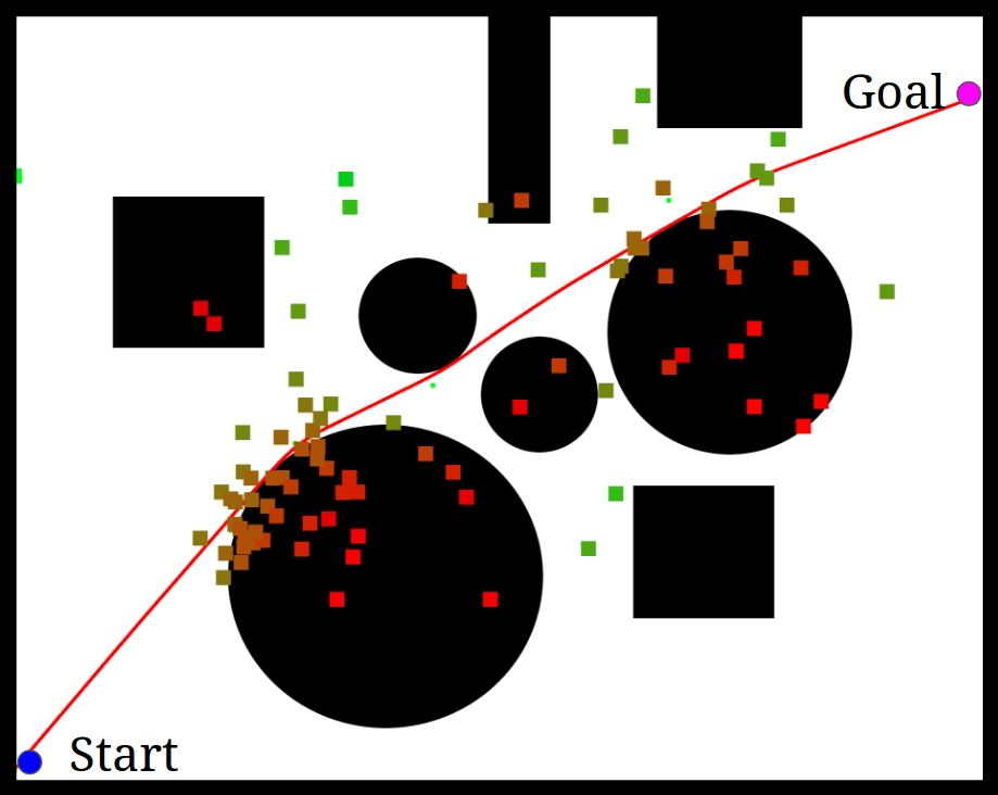
(a)

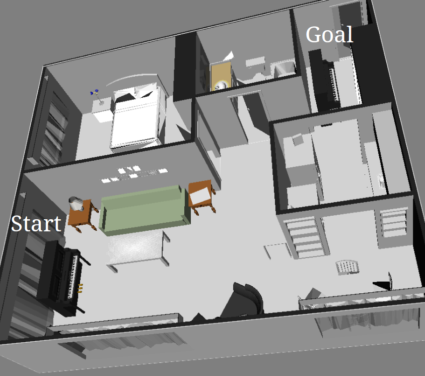
(b)

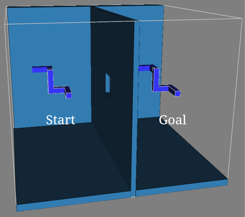
(c)

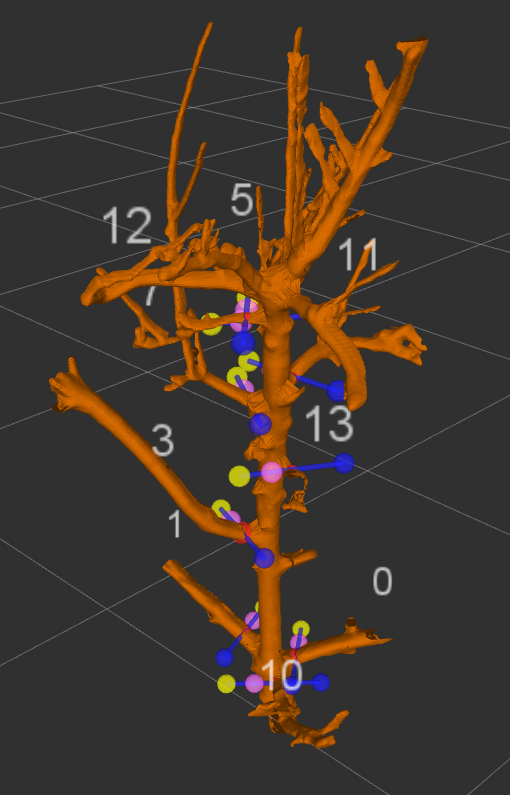
(d)

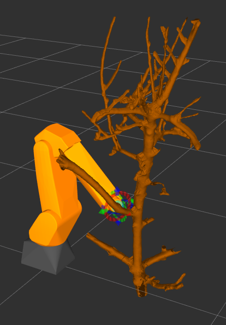
(e)

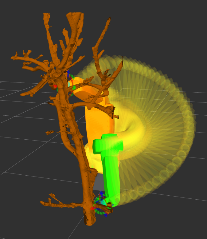
(f)

Figure 2: Spatial layouts for the four benchmarks and selected results. (a) A sample solution by cRMPD on the 2D bitmap. The approximated clearance cost of a sample is indicated by the color. (b) The Piano Mover’s problem. (c) The Twistcooler Problem. (d) Mesh of the scanned apple tree. To prune a branch, the end effector must reach the pink marker while staying aligned to the blue arrow. (e) An example pruning pose used in the benchmark. (f) An example path found by cRMPD.

4.2 Point Robot on 2D Bitmap

The point robot, with 2 translational DoF, in the bitmap case studied by us must navigate from the bottom left corner of the map to the top right corner, as shown in Figure 2(a). The environment contains a cluster of obstacles that are placed to form a narrow direct passage to the goal along the diagonal, while creating an open region near the bottom right corner. In this benchmark, every run is given a 0.5s quantum, which is sufficient for the cost of RRT* to converge. Through the quantitative results in Table 1, we observe that although RRT and RRT-Connect score higher with regard to planning time, they are likely to choose suboptimal path segments in the open regions of the configuration space. This observation is best supported by the comparison on path lengths. On the other hand, navigating through the narrow diagonal passage poses little challenge for the cRMPD planner. With a straight line initialization, cRMPD achieves a competitive average path length comparable to what is returned by RRT* although RRT* takes more than 10 times longer to find the path. Also note that our state-dependent cost function allows cRMPD to save on the number of collision checks.

Table 1: 2D point robot benchmark results. Every column is normalized against the best performer to extract the relative performance (# CC = number of collision checks).

	Time	Length	# CC
RRT	1.07	1.15	1.36
RRT-C	1.00	1.15	1.23
RRT*	427.34	1.00	43.28
cRMPD	31.84	1.03	1.00

4.3 Path Planning in 3D Workspaces

To examine the characteristics of cRMPD in 3D workspaces, we study two rigid-body motion planning problems. The set of transformations for all rigid-body motions in 3D workspaces forms the special Euclidean manifold, $SE(3)$. This manifold spans a 6-dimensional space consisting of two subspaces: a 3D Euclidean space for translations and another 3D space in the special Orthogonal group $SO(3)$ that describes rotations.

It is noteworthy that the distance between any two points on the $SE(3)$ manifold is defined as a simple summation of distances in the two subspaces: $\ell_{2}$-norm in the Euclidean subspace and arc-length on the $SO(3)$ manifold (?). To avoid the complications created by averaging the states in $SE(3)$, as required by the EGD (estimated gradient descent) calculation in line 10 of Algorithm 2, cRMPD adopts a greedy strategy for choosing the middle point – the updated middle point in each iteration is simply the one with the lowest cost among the $K$ samples. As the reader will see shortly, this works well in practice.

Of the two 3D path planning problems we first show results for the classic Piano Mover’s problem, as seen in Figure 2(c), where a piano must be maneuvered through the living room and the narrow corridor at the top right. The results, presented in Table 2, show that cRMPD surpasses its competitors by a significant margin with respect to nearly all the metrics. While being more than 10 times faster than RRT-Connect, cRMPD still returns the shortest and smoothest path, even compared to the optimal planner RRT*.

Table 2: Relative performance for the Piano Mover’s problem (SR = Success Rate and $q_{smt}$ = Smoothness Cost).

	Time	Length	$q_{smt}$	# CC	SR (%)
RRT	32.74	1.25	8.75	71.46	80.0
RRT-C	15.17	1.22	7.78	38.55	100.0
RRT*	61.35	1.02	8.01	186.28	73.3
PRM	37.62	1.21	9.20	137.29	76.7
cRMPD	1.00	1.00	1.00	1.00	96.7

In the second 3D path planning problem, the Twistcooler problem, a 5-link rigid-body robot must navigate through a small hole in a barrier in the middle while there exist large open spaces on the two sides of the barrier. The Twistcooler problem is deceivingly challenging: the small hole in the middle and the stretched shape of the robot form a elongated narrow passage in the configuration space. For RRT and its variants, a typical run lasts several hundreds of seconds before a solution is found. We did try to combine those planners with obstacle-based samplers that generate samples close to obstacles, yet no major improvement in planning time was observed. The PRM planner achieved the highest success rate and improved time efficiency, however it did so with compromised path smoothness and the most number of collision checks.

As shown by the benchmarking results tabulated in Table 3, cRMPD possesses superior ability to navigate through narrow passages. Quantitatively speaking, cRMPD is able to produce a path within a time span that is one order of magnitude shorter than any other planner. In addition, cRMPD is able to do so without compromising the path quality, as demonstrated the final solution length and smoothness.

Table 3: Relative performance for the Twistcooler problem.

	Time	Length	$q_{smt}$	# CC	SR (%)
RRT	279.01	1.49	16.23	430.05	96.7
RRT-C	428.22	1.55	15.49	665.52	73.3
RRT*	746.27	1.00	11.74	152.96	60.0
PRM	52.81	1.52	21.62	882.87	100.0
cRMPD	1.00	1.00	1.00	1.00	90.0

4.4 Dormant Apple Tree Pruning

Table 4: Relative performance on the tree pruning benchmark.

	Time	Length	$q_{smt}$	SR (%)
RRT	17.28	1.47	2.16	91.5
RRT-C	1.00	1.12	15.49	100.0
RRT*	37.55	1.19	1.34	93.1
STOMP	24.75	1.00	1.00	41.5
cRMPD	1.81	1.07	1.68	100.0

We now show results for a real-world problem: dormant apple tree pruning with a 6-DoF robot arm. The mesh of the tree is obtained by scanning a real dormant tree using an RGB-D sensor. To prune a branch, the end effector of the robot arm must reach the base of that branch in a perpendicular direction, as demonstrated by the example pruning pose in Figure 2(e). This benchmark consists of 13 queries in total and each planner is tasked to solve the query 10 times with a maximum allowable time of 5s. Interestingly, the thin spindly trees would present challenges in the form of non-convex cost surfaces for any optimization-based planner, including STOMP and cRMPD. In the case of cRMPD, our experiments have shown that when the EGD begins with a naive middle point initialization, namely $p_{m}=(p_{s}+p_{g})/2$, subsequent middle points often descend quickly into a local minimum that is not collision-free, resulting in a failure of the planner. Along similar lines, the consequence of this non-convexity is also reflected in the low success rate of STOMP, shown in Table 4. To address this shortcoming, a high-quality initialization is of crucial importance. Therefore, before the invocation of $CostAwareFreeStateSampler$, cRMPD first takes $K$ samples around the middle point and compute their costs. Subsequently, the seed point $p_{m}$ that is being passed to the $CostAwareFreeStateSampler$ call is the one with the lowest cost among the $K$ samples.

The greedy initialization strategy of cRMPD as described above has been shown to work effectively. As one can tell from the results in Table 4, the trade-off between time efficiency and path quality is evident. Whereas STOMP offers the best path quality, it is prone to failure and entails a large computational burden. The opposite of this conclusion holds true for RRT-Connect. On the other hand, cRMPD offers us a better trade-off between path quality and computational burden. Not only can cRMPD answer the queries with a 100% success rate, it also achieves near optimum performance in terms of planning time and path length.

4.5 Limitations

Despite out-performing the other well-known planners in our comparative study, cRMPD has some limitations of its own. First, if a middle point is chosen poorly, it will cause subsequent middle points to diverge from the optimal path. Since cRMPD is a single-path planner, a middle point, once chosen, can no longer be changed in later iterations and remains in the final path. We believe that this shortcoming could be addressed by using cRMPD only as a local planner in a probabilistically complete top-level planner, such as RRT. Furthermore, launching multiple instances of cRMPD simultaneously in a multi-threaded fashion also would help get around the difficulties that may arise with the possible suboptimality of the middle points.

5 Conclusion

Best known randomized sampling based algorithms for path planning, while possessing the highly desirable property of probabilistic completeness, unfortunately tend to carry out unnecessary randomized explorations in open spaces and branch out slowly in narrow passages. Our “local” planner RMPD has the ability to efficiently bypass local obstacles using inexpensive resampling, which accelerates excursions into narrow passages through a divide-and-conquer strategy. Additionally, cRMPD, our cost-aware version of RMPD, takes advantage of estimated gradient descent to produce a cost-optimal middle point. cRMPD uses a Monte Carlo sampling strategy where the current sampling distribution is constantly steered to low-cost samples in the previous iteration. Our experimental results demonstrate that cRMPD possesses superior qualities with regard to time efficiency and path quality. This makes cRMPD a powerful new approach to path planning.

6 Acknowledgement

The authors would like to thank the anonymous reviewers for their insightful feedback. This project was supported by the USDA Specialty Crop Research Initiative (SCRI).

References

- [Barraquand and Latombe 1993] Barraquand, J., and Latombe, J.-C. 1993. Nonholonomic multibody mobile robots: Controllability and motion planning in the presence of obstacles. Algorithmica 10(2-4):121.
- [Clifton et al. 2008] Clifton, M.; Paul, G.; Kwok, N.; Liu, D.; and Wang, D.-L. 2008. Evaluating performance of multiple RRTs. In Mechtronic and Embedded Systems and Applications, 2008. MESA 2008. IEEE/ASME International Conference on, 564–569. IEEE.
- [Elbanhawi and Simic 2014] Elbanhawi, M., and Simic, M. 2014. Sampling-based robot motion planning: A review. IEEE Access 2:56–77.
- [Hsu et al. 2003] Hsu, D.; Jiang, T.; Reif, J.; and Sun, Z. 2003. The bridge test for sampling narrow passages with probabilistic roadmap planners. In Robotics and Automation, 2003. Proceedings. ICRA’03. IEEE International Conference on, volume 3, 4420–4426. IEEE.
- [Kalakrishnan et al. 2011] Kalakrishnan, M.; Chitta, S.; Theodorou, E.; Pastor, P.; and Schaal, S. 2011. STOMP: Stochastic trajectory optimization for motion planning. In Robotics and Automation (ICRA), 2011 IEEE International Conference on, 4569–4574. IEEE.
- [Kalakrishnan 2011] Kalakrishnan, M. 2011. STOMP motion planner. http://wiki.ros.org/stomp_motion_planner. Accessed: 2017-11-20.
- [Karaman and Frazzoli 2011] Karaman, S., and Frazzoli, E. 2011. Sampling-based algorithms for optimal motion planning. The international journal of robotics research 30(7):846–894.
- [Kavraki et al. 1996] Kavraki, L. E.; Svestka, P.; Latombe, J.-C.; and Overmars, M. H. 1996. Probabilistic roadmaps for path planning in high-dimensional configuration spaces. IEEE transactions on Robotics and Automation 12(4):566–580.
- [Kuffner and LaValle 2000] Kuffner, J. J., and LaValle, S. M. 2000. RRT-connect: An efficient approach to single-query path planning. In Robotics and Automation, 2000. Proceedings. ICRA’00. IEEE International Conference on, volume 2, 995–1001. IEEE.
- [Kuffner 2004] Kuffner, J. J. 2004. Effective sampling and distance metrics for 3d rigid body path planning. In Robotics and Automation, 2004. Proceedings. ICRA’04. 2004 IEEE International Conference on, volume 4, 3993–3998. IEEE.
- [Kuwata et al. 2009] Kuwata, Y.; Teo, J.; Fiore, G.; Karaman, S.; Frazzoli, E.; and How, J. P. 2009. Real-time motion planning with applications to autonomous urban driving. IEEE Transactions on Control Systems Technology 17(5):1105–1118.
- [LaValle 1998] LaValle, S. M. 1998. Rapidly-exploring random trees: A new tool for path planning.
- [Lee et al. 2012] Lee, J.; Kwon, O.; Zhang, L.; and Yoon, S.-e. 2012. SR-RRT: Selective retraction-based rrt planner. In Robotics and Automation (ICRA), 2012 IEEE International Conference on, 2543–2550. IEEE.
- [Nof 1999] Nof, S. Y. 1999. Handbook of industrial robotics, volume 1. John Wiley & Sons.
- [Ratliff et al. 2009] Ratliff, N.; Zucker, M.; Bagnell, J. A.; and Srinivasa, S. 2009. CHOMP: Gradient optimization techniques for efficient motion planning. In Robotics and Automation, 2009. ICRA’09. IEEE International Conference on, 489–494. IEEE.
- [Sucan and Chitta 2011] Sucan, I. A., and Chitta, S. 2011. MoveIt! http://moveit.ros.org.
- [Sucan, Moll, and Kavraki 2012] Sucan, I. A.; Moll, M.; and Kavraki, L. E. 2012. The open motion planning library. IEEE Robotics & Automation Magazine 19(4):72–82.
- [Urmson and Simmons 2003] Urmson, C., and Simmons, R. 2003. Approaches for heuristically biasing RRT growth. In Intelligent Robots and Systems, 2003.(IROS 2003). Proceedings. 2003 IEEE/RSJ International Conference on, volume 2, 1178–1183. IEEE.
- [Zhang and Manocha 2008] Zhang, L., and Manocha, D. 2008. An efficient retraction-based RRT planner. In Robotics and Automation, 2008. ICRA 2008. IEEE International Conference on, 3743–3750. IEEE.