Iteratively Linearized Reweighted Alternating Direction Method of Multipliers for a Class of Nonconvex Problems
Abstract
In this paper, we consider solving a class of nonconvex and nonsmooth problems frequently appearing in signal processing and machine learning research. The traditional alternating direction method of multipliers encounters troubles in both mathematics and computations in solving the nonconvex and nonsmooth subproblem. In view of this, we propose a reweighted alternating direction method of multipliers. In this algorithm, all subproblems are convex and easy to solve. We also provide several guarantees for the convergence and prove that the algorithm globally converges to a critical point of an auxiliary function with the help of the Kurdyka-Łojasiewicz property. Several numerical results are presented to demonstrate the efficiency of the proposed algorithm.
Keywords: Alternating direction method of multipliers; Iteratively reweighted algorithm; Nonconvex and nonsmooth minimization; Kurdyka-Łojasiewicz property; Semi-algebraic functions
Mathematical Subject Classification 90C30, 90C26, 47N10
1 Introduction
Minimization of composite functions with linear constrains finds various applications in signal and image processing, statistics, machine learning, to name a few. Mathematically, such a problem can be presented as
| (1.1) |
where , , and is usually the regularization function, and is usually the loss function.
The well-known alternating direction method of multipliers (ADMM) method [1, 2] is a powerful tool for the problem mentioned above. The ADMM actually focuses on the augmented Lagrangian problem of (1.1) which reads as
| (1.2) |
where is a parameter. The ADMM minimizes only one variable and fixes others in each iteration; the variable is updated by a feedback strategy. Mathematically, the standard ADMM method can be presented as
| (1.6) |
The ADMM algorithm attracts increasing attention for its efficiency in dealing with sparsity-related problems [3, 4, 5, 6, 7]. Obviously, the ADMM has a self-explanatory assumption; all the subproblems shall be solved efficiently. In fact, if the proximal maps of the and are easy to calculate, the linearized ADMM [8] proposes the linearized technique to solve the subproblem efficiently; the subproblems all need to compute proximal map of or once. The core part of the linearized ADMM lies in linearizing the quadratic terms and in each iteration. The linearized ADMM is also called as preconditioned ADMM in [9]; in fact, it is also a special case when in Chambolle-Pock primal dual algorithm [10]. In the latter paper [11], the linearized ADMM is further generalized as the Bregman ADMM.
The convergence of the ADMM in the convex case is also well studied; numerous excellent works have made contributions to this field [12, 13, 14, 15]. Recently, the ADMM algorithm is even developed for the infeasible problems [16, 17]. The earlier analyses focus on the convex case, i.e., both and are all convex. But as the nonconvex penalty functions perform efficiently in applications, nonconvex ADMM is developed and studied: in paper [18], Chartrand and Brendt directly used the ADMM to the group sparsity problems. They replace the nonconvex subproblems as a class of proximal maps. Later, Ames and Hong consider applying ADMM for certain non-convex quadratic problems [19]. The convergence is also presented. A class of nonconvex problems is solved by Hong et al by a provably convergent ADMM [20]. They also allow the subproblems to be solved inexactly by taking gradient steps which can be regarded as a linearization. Recently, with weaker assumptions, [21] present new analysis for nonconvex ADMM by novel mathematical techniques. With the Kurdyka-Łojasiewicz property, [22, 23] consider the convergence of the generated iterative points. [24] considered a structured constrained problem and proposed the ADMM-DC algorithm. In nonconvex ADMM literature, either the proximal maps of and or the subproblems are assumed to be easily solved.
1.1 Motivating example and problem formulation
This subsection contains two parts: the first one presents an example and discusses the problems in direct using the ADMM; the second one describes the problem considered in this paper.
1.1.1 A motivating example: the problems in directly using ADMM
The methods mentioned above are feasibly applicable provided the subproblems are relatively easy to solve, i.e., either the proximal maps of and or the subproblems are assumed to be easily solved. However, the nonconvex cases may not always promise such a convention. We recall the problem [25] which arises in imaging science
| (1.7) |
where is the total variation operator and . By denoting , the problem then turns to being
| (1.8) |
The direct ADMM for this problem can be presented as
| (1.12) |
The first subproblem in the algorithm needs to minimize a nonconvex and nonsmooth problem. If , the point can be explicitly calculated. This is because the proximal map of can be easily obtained. But for other , the proximal map cannot be easily derived. Thus, we may must employ iterative algorithms to compute . That indicates three drawbacks which cannot be ignored:
-
1.
The stopping criterion is hard to set for the nonconvexity111The convex methods usually enjoy a convergence rate..
-
2.
The error may be accumulating in the iterations due to the inexact numerical solution of the subproblem.
-
3.
Even the subproblem can be numerically solved without any error, the numerical solution for the subproblem is always a critical point rather than the “real” argmin due to the nonconvexity.
1.1.2 Optimization problem and basic assumptions
In this paper, we consider the following problem
| (1.13) |
where , and , and satisfy the following assumptions:
A.1 is a differentiable convex function with a Lipschitz continuous gradient, i.e.,
| (1.14) |
And the function is strongly convex with constant .
A.2 is convex and proximable.
A.3 is a differentiable concave function with a Lipschitz continuous gradient whose Lipschitz continuity modulus is bounded by ; that is
| (1.15) |
and when .
1.2 Linearized ADMM meets the iteratively reweighted strategy: convexifying the subproblems
In this part, we present the algorithm for solving problem (1.13). The term has a deep relationship with several iteratively reweighted style algorithms [30, 31, 32, 33, 34]. Although the function may be nondifferentiable itself, the reweighted style methods still propose an elegant way: linearization of outside function . Precisely, in -th iteration of the iteratively reweighted style algorithms, the term is usually replaced by , where is obtained in the -th iteration. The extensions of reweighted style methods to matrix cases are considered and analyzed in [35, 36, 37, 38, 39]. In fact, the iteratively reweighted technique is a special majorization minimization technique, which has also been adopted in ADMM [40]. Compared with [40], the most difference in our paper is the exploiting the specific structure of the problem in nonconvex settings. Motivated by the iteratively reweighted strategy, we propose the following scheme for solving (1.13)
| (1.20) |
We combined both linearized ADMM and reweighted algorithm in the new scheme: for the nonconvex part , we linearize the outside function and keep , which aims to derive the convexity of the subproblem; for the quadratic part , linearization is for the use of the proximal map of . We call this new algorithm as Iteratively Linearized Reweighted Alternating Direction Method of Multipliers (ILR-ADMM). It is easy to see that each subproblem just needs to solve a convex problem in this scheme. With the expression of proximal maps, updating can be equivalently presented as the following forms
| (1.21) |
where , and denotes the -th column of the matrix . In many applications, is the quadratic function, and then solving is also very easy. With this form, the algorithm can be programmed with the absence of the inner loop.
1.3 Contribution and Organization
In this paper, we consider a class of nonconvex and nonsmooth problems which are ubiquitous in applications. Direct use of ADMM algorithms will lead to troubles in both computations and mathematics for the nonconvexity of the subproblem. In view of this, we propose the iteratively linearized reweighted alternating direction method of multipliers for these problems. The new algorithm is a combination of iteratively reweighted strategy and the linearized ADMM. All the subproblems in the proposed algorithm are convex and easy to solve if the proximal map of is easy to solve and is quadratic. Compared with the direct application of ADMM to problem (1.13), we now list the advantages of the new algorithm:
-
1.
Computational perspective: each subproblem just needs to compute once proximal map of and minimize a quadratic problem, the computational cost is low in each iteration.
-
2.
Practical perspective: without any inner loop, the programming is very easy.
-
3.
Mathematical perspective: all the subproblems is convex and exactly solved. Thus, we get “real” argmin everywhere, which makes the mathematical convergence analysis solid and meaningful.
With the help of the Kurdyka-Łojasiewicz property, we provide the convergence results of the algorithm with proper selections of the parameters. The applications of the new algorithm to the signal and image processing are presented. The numerical results demonstrate the efficiency of the proposed algorithm.
The rest of this paper is organized as follows. Section 2 introduces the preliminaries including the definitions of subdifferential and the Kurdyka-Łojasiewicz property. Section 3 provides the convergence analysis. The core part is using an auxiliary Lyapunov function and bounding the generated sequence. Section 4 applies the proposed algorithm to image deblurring. And several comparisons are reported. Finally, Section 5 concludes the paper.
2 Preliminaries
We introduce the basic tools in the analysis: the subdifferential and Kurdyka-Łojasiewicz property. These two definitions play important roles in the variational analysis.
2.1 Subdifferential
Given a lower semicontinuous function , its domain is defined by
The graph of a real extended valued function is defined by
Now, we are prepared to present the definition of subdifferential. More details can be found in [41].
Definition 1.
Let be a proper and lower semicontinuous function.
-
1.
For a given , the Frchet subdifferential of at , written as , is the set of all vectors satisfying
When , we set .
-
2.
The (limiting) subdifferential, or simply the subdifferential, of at , written as , is defined through the following closure process
Note that if , . When is convex, the definition agrees with the subgradient in convex analysis [42] which is defined as
It is easy to verify that the Frchet subdifferential is convex and closed while the subdifferential is closed. Denote that
thus, is a closed set. Let be a sequence in such that . If converges to as and converges to as , then . This indicates the following simple proposition.
Proposition 1.
If , , , , and 222If is continuous, the condition certainly holds if .. Then, we have
| (2.1) |
Definition 2.
A point that satisfies (2.2) is called (limiting) critical point. The set of critical points of is denoted by .
Proposition 2.
Proof.
With [Proposition 10.5, [41]], we have
| (2.3) |
Noting that is differentiable and is convex, with direct computation, we have
| (2.4) |
And more, by definition, we can obtain
| (2.5) |
We then prove the first equation. The second and third are quite easy. ∎
2.2 Kurdyka-Łojasiewicz function
The domain of a subdifferential is given as
Definition 3.
(a) The function is said to have the Kurdyka-Łojasiewicz property at if there exist , a neighborhood of and a continuous concave function such that
-
1.
.
-
2.
is on .
-
3.
for all , .
-
4.
for all in , it holds
(2.6)
(b) Proper closed functions which satisfy the Kurdyka-Łojasiewicz property at each point of are called KL functions.
More details can be found in [43, 44, 45]. In the following part of the paper, we use KL for Kurdyka-Łojasiewicz for short. Directly checking whether a function is KL or not is hard, but the proper closed semi-algebraic functions [45] do much help.
Definition 4.
(a) A subset of is a real semi-algebraic set if there exists a finite number of real polynomial functions such that
(b) A function is called semi-algebraic if its graph
is a semi-algebraic subset of .
Better yet, the semi-algebraicity enjoys many quite nice properties and various kinds of functions are KL [46]. We just put a few of them here:
-
•
Real closed polynomial functions.
-
•
Indicator functions of closed semi-algebraic sets.
-
•
Finite sums and product of closed semi-algebraic functions.
-
•
The composition of closed semi-algebraic functions.
-
•
Sup/Inf type function, e.g., is semi-algebraic when is a closed semi-algebraic function and a closed semi-algebraic set.
-
•
Closed-cone of PSD matrices, closed Stiefel manifolds and closed constant rank matrices.
Lemma 1 ([45]).
Let be a proper and closed function. If is semi-algebraic then it satisfies the KL property at any point of .
The previous definition and property of KL is about a certain point in . In fact, the property has been extended to a certain closed set [47]. And this property makes previous convergence proofs related to KL property much easier.
Lemma 2.
Let be a proper lower semi-continuous function and be a compact set. If is a constant on and satisfies the KL property at each point on , then there exists concave function satisfying the four properties given in Definition 3 and such that for any and any satisfying that and , it holds that
| (2.7) |
3 Convergence analysis
In this part, the function is defined in (1.16). We provide the convergence guarantee and the convergence analysis of ILR-ADMM (Algorithm 1). We first present a sketch of the proofs, which is also a big picture for the purpose of each lemma and theorem:
-
•
In the first step, we bound the dual variables by the primal points (Lemma 3).
-
•
In the second step, the sufficient descent condition is derived for a new Lyapunov function (Lemma 4).
-
•
In the third step, we provide several conditions to bound the points (Lemma 5).
-
•
In the fourth step, the relative error condition is proved (Lemma 6).
-
•
In the last step, we prove the convergence under semi-algebraic assumption (Theorem 1).
The proofs in our paper are closely related to seminal papers [20, 21, 22] in several proofs treatments. In fact, some proofs follow their techniques. For example, in Lemma 3, we employ the method used in [Lemma 3, [21]] to bound . In Lemma 5, boundedness of the sequence is also proved by a similar way given in [Theorem 3, [22]]. Besides the detailed issues, in the large picture, the keystones are also similar to [20, 21, 22]: we also prove the sufficient descent and subdifferential bound for a Lyapunov function, and the boundedness of the generated points.
However, the proofs in our paper are still different from [20, 21, 22] in various aspects. The novelties mainly lay in deriving the sufficient descent and subdifferential bound based on the specific structure of our problem. Noting that in each iteration, we minimize and rather than and . Thus, the previous methods cannot be directly used in our paper. By exploiting the structure property of the problem, we built these two conditions.
Lemma 3.
If
| (3.1) |
Then, we have
| (3.2) |
where , and is the smallest strictly-positive eigenvalue of .
Proof.
The second step in each iteration actually gives
| (3.3) |
With the expression of ,
| (3.4) |
Replacing with , we can obtain
| (3.5) |
Under condition (3.1), ; and subtraction of the two equations above gives
| (3.6) |
∎
Remark 1.
Remark 2.
The condition (3.1) is satisfied if is surjective. However, in many applications, the matrix may fail to be surjective. For example, for a matrix , we consider the operator
| (3.8) |
where is the forward difference operator. Noting the when , thus, cannot be surjective in this case. However, the current convergence of nonconvex ADMM is all based on the surjective assumption on or condition (3.1), which is also used in our analysis. How to remove condition (3.1) in the nonconvex ADMM deserves further research.
Now, we introduce several notation to present the following lemma. Denote the variable and the sequence as
| (3.9) |
An auxiliary function is always used in the proof
| (3.10) |
Lemma 4 (Descent).
Let the sequence be generated by ILR-ADMM. If condition (3.1) and the following condition
| (3.11) |
hold, then there exists such that
| (3.12) |
where .
Proof.
Direct calculation shows that the first step is actually minimizing the function with respect to . Thus, we have
Similarly, actually minimizes . Noting , with assumption A.1, the strongly convex constant of is larger than ,
| (3.13) |
Direct calculation yields
| (3.14) |
Combining the equations above, we can have
| (3.15) |
Noting is concave, we have
| (3.16) | ||||
Then, we can derive
With Lemma 3, we then have
| (3.17) |
Letting , we then prove the result. ∎
In fact, condition (3.11) can be always satisfied in applications because the parameters and are both selected by the user. Different with the ADMMs in convex setting, the parameter is nonarbitrary, the here should be sufficiently large.
Lemma 5 (Boundedness).
If and conditions (3.1) and (3.11) hold, and there exists such that
| (3.18) |
and
| (3.19) |
The sequence is bounded, if one of the following conditions holds:
B1. is coercive, and is coercive.
B2. is coercive, and is invertible.
B3. , is coercive, and is invertible.
Proof.
We have
| (3.20) |
Noting is decreasing with Lemma 4, . We then can see , , are all bounded. It is easy to see that if one of the three conditions holds, will be bounded. ∎
Remark 3.
Remark 4.
Both assumptions B2 and B3 actually imply condition (3.7).
Remark 5.
Lemma 6 (Relative error).
Proof.
Due to that is convex, is Lipschitz continuous with some constant if being restricted to some bounded set. Thus, there exists such that
Updating in each iteration certainly yields
| (3.23) |
where and . Noting the boundedness of the sequence and , the continuity of indicates there exist such that
| (3.24) |
Easy computation gives
| (3.25) |
With the boundedness of the generated points, there exist such that
| (3.26) |
Thus, we have
| (3.27) |
Obviously, it holds that
Thus, with Lemma 3, we derive that
| (3.28) |
for . From the second step in each iteration,
| (3.29) |
Direct calculation gives
| (3.30) |
That is also
| (3.31) |
With Lemma 3, we have
where . It is easy to see
| (3.32) |
And we have
| (3.33) |
for . With the deductions above,
| (3.34) |
Denoting , we then finish the proof. ∎
Lemma 7.
If the sequence is bounded and conditions of Lemma 6 hold, then we have
| (3.35) |
For any cluster point , it is also a critical point of .
Proof.
We can easily see that is also bounded. The continuity of indicates that is bounded. From Lemma 4, is decreasing. Thus, the sequence is convergent, i.e., . With Lemma 4, we have
| (3.36) |
From the scheme of the ILR-ADMM, we also have
| (3.37) |
For any cluster point , there exists such that . Then, we further have . From Lemma 3, we also have . That also means
| (3.38) |
From the scheme, we have the following conditions
Letting , with Proposition 1, we have
The first relation above is actually . From Proposition 2, is a critical point of . ∎
In the following, to prove the convergence result, we first establish some results about the limit points of the sequence generated by ILR-ADMM. These results are presented for the use of Lemma 2. We recall a definition of the limit point which is introduced in [47].
Definition 5.
Define that
where is an arbitrary starting point.
Lemma 8.
Suppose that the conditions of Lemma 6 hold, and is generated by scheme (1.20). Then, we have the following results.
(1) is nonempty and .
(2) .
(3) is finite and constant on .
Proof.
(1) Due to that is bounded, is nonempty. Assume that , from the definition, there exists a subsequence . From Lemma 4, we have . From Lemma 6, there exists and . Proposition 1 indicates that , i.e. .
(2) This item follows as a consequence of the definition of the limit point.
(3) The continuity of directly yields this result. ∎
Theorem 1 (Convergence result).
Proof.
Obviously, is also semi-algebraic. And with Lemma 1, is KL. From Lemma 8, is constant on . Let be a stationary point of . Also from Lemma 8, we have and if any for some . If for some , , that is . With Lemma 8, when . Thus, with Lemma 4, when . If for any , with Lemma 2, we have
| (3.40) |
which together with Lemma 6 gives
| (3.41) |
Then, the concavity of yields
With Lemma 4, we have
which is equivalent to
| (3.42) |
Using the Schwartz’s inequality, we then derive that
| (3.43) |
That is also
| (3.44) |
Summing (3.44) from to yields that
| (3.45) |
Letting , we have
| (3.46) |
From Lemma 8, there exists a critical point of . Then, is convergent and is a stationary point of . That is to say converges to . Note that is a linear composition of and , thus converges to . ∎
4 Applications and numerical results
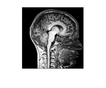
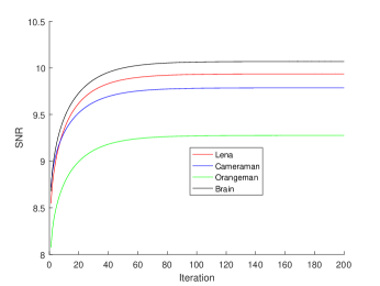
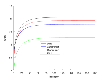
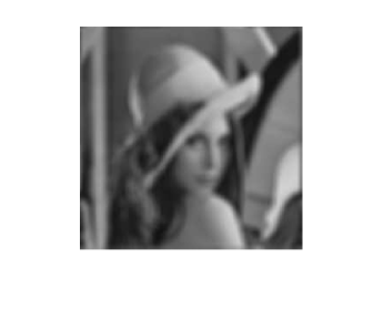
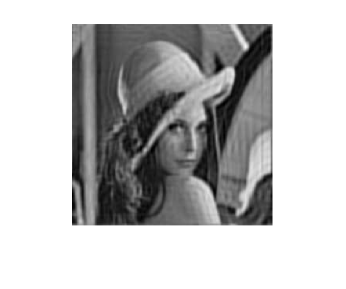
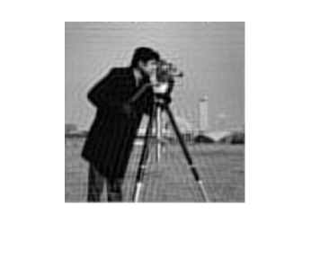
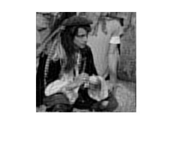
In this part, we consider applying ILR-ADMM to problem (1.7) for image deblurring. This section contains two parts: in the first one, several basic properties of the proposed algorithm, such as the convergence and the influence of the selection of the parameter in problem (1.7), are investigated; in the second one, the proposed algorithm is compared with other classical methods for image deblurring. We employ four images (see Figure 1), which include three nature images, one MRI image for our numerical experiments. The performance of the deblurring algorithms is quantitatively measured by means of the signal-to-noise ratio (SNR)
| (4.1) |
where and denote the original image and the restored image, respectively, and represents the mean of the original image .


In the experiments, we use an increasing technique for the parameter in ILR-ADMM, i.e., , with and upper bound . Such a technique has been used for ADMM in [49]. From (3.21), we need ; and it is set as . For all the algorithms used in this section, the initialization is the blurred image.
4.1 Performance of ILR-ADMM
In this subsection, we focus on the convergence of ILR-ADMM. The blurring operator used for our experiments are generated
by the matlab command fspecial(’gaussian’,17,5). And in the problem (1.7), we choose .
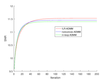
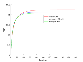
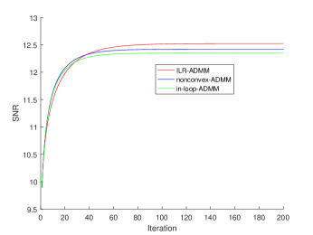
For , we apply ILR-ADMM to reconstruct the four images in Figure 1. We run all the algorithms 10 times in each case and then take the average. Fig. 2 shows the SNR versus the iterations and the maximum iteration is 200.
4.2 Comparisons with other classical methods
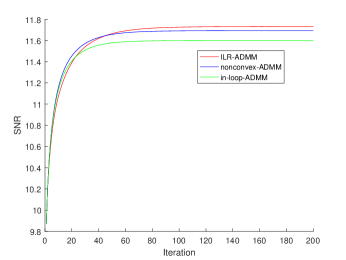
This subsection focuses on for problem (1.7). We consider two algorithms for comparisons: the first one is the direct nonconvex ADMM; the second one considers using an inner loop for the subproblem. Precisely, the inner loop is constructed by the proximal reweighted algorithm. And in the numerical examples, the inner loop is set as 10. We call this algorithm as in-loop-ADMM.
The blurring operator is generated by the Matlab commands fspecial(’gaussian’,.,.). The parameter is set as , is generated by the Gaussian noise . Fig. 3, 4, 5 and 6 present the reconstructed images with different algorithms for the four images in Fig. 1. The maximum iteration is set as 200. We run all algorithms ten times and take the average. The time cost (T) is also reported. We also plot the SNR versus the iteration for different algorithms in each image. From numerical results, we can see ILR-ADMM perform better than the nonconvex ADMM with almost same time cost. Due to that in-loop-ADMM employs the inner loop, the time cost is much larger than ILR-ADMM. In general, ILR-ADMM outperforms than the other two algorithms.


5 Conclusion
In this paper, we consider a class of nonconvex and nonsmooth minimizations with linear constraints which have applications in signal processing and machine learning research. The classical ADMM method for these problems always encounters both computational and mathematical barriers in solving the subproblem. We combined the reweighted algorithm and linearized techniques, and then designed a new ADMM. In the proposed algorithm, each subproblem just needs to calculate the proximal maps. The convergence is proved under several assumptions on the parameters and functions. And numerical results demonstrate the efficiency of our algorithm.
References
- [1] D. Gabay and B. Mercier, “A dual algorithm for the solution of nonlinear variational problems via finite element approximation,” Computers & Mathematics with Applications, vol. 2, no. 1, pp. 17–40, 1976.
- [2] R. Glowinski and A. Marroco, “Sur l’approximation, par éléments finis d’ordre un, et la résolution, par pénalisation-dualité d’une classe de problèmes de dirichlet non linéaires,” Revue française d’automatique, informatique, recherche opérationnelle. Analyse numérique, vol. 9, no. R2, pp. 41–76, 1975.
- [3] J. Yang, Y. Zhang, and W. Yin, “A fast alternating direction method for tvl1-l2 signal reconstruction from partial fourier data,” IEEE Journal of Selected Topics in Signal Processing, vol. 4, no. 2, pp. 288–297, 2010.
- [4] Z. Wen, D. Goldfarb, and W. Yin, “Alternating direction augmented lagrangian methods for semidefinite programming,” Mathematical Programming Computation, vol. 2, no. 3, pp. 203–230, 2010.
- [5] Y. Xu, W. Yin, Z. Wen, and Y. Zhang, “An alternating direction algorithm for matrix completion with nonnegative factors,” Frontiers of Mathematics in China, vol. 7, no. 2, pp. 365–384, 2012.
- [6] M. K. Ng, P. Weiss, and X. Yuan, “Solving constrained total-variation image restoration and reconstruction problems via alternating direction methods,” SIAM journal on Scientific Computing, vol. 32, no. 5, pp. 2710–2736, 2010.
- [7] Y. Wang, J. Yang, W. Yin, and Y. Zhang, “A new alternating minimization algorithm for total variation image reconstruction,” SIAM Journal on Imaging Sciences, vol. 1, no. 3, pp. 248–272, 2008.
- [8] G. Chen and M. Teboulle, “A proximal-based decomposition method for convex minimization problems,” Mathematical Programming, vol. 64, no. 1-3, pp. 81–101, 1994.
- [9] E. Esser, X. Zhang, and T. F. Chan, “A general framework for a class of first order primal-dual algorithms for convex optimization in imaging science,” SIAM Journal on Imaging Sciences, vol. 3, no. 4, pp. 1015–1046, 2010.
- [10] A. Chambolle and T. Pock, “A first-order primal-dual algorithm for convex problems with applications to imaging,” Journal of mathematical imaging and vision, vol. 40, no. 1, pp. 120–145, 2011.
- [11] H. Wang and A. Banerjee, “Bregman alternating direction method of multipliers,” in Advances in Neural Information Processing Systems, pp. 2816–2824, 2014.
- [12] B. He and X. Yuan, “On the o(1/n) convergence rate of the douglas–rachford alternating direction method,” SIAM Journal on Numerical Analysis, vol. 50, no. 2, pp. 700–709, 2012.
- [13] B. He and X. Yuan, “On non-ergodic convergence rate of douglas–rachford alternating direction method of multipliers,” Numerische Mathematik, vol. 130, no. 3, pp. 567–577, 2015.
- [14] M. Hong and Z.-Q. Luo, “On the linear convergence of the alternating direction method of multipliers,” Mathematical Programming, vol. 162, no. 1-2, pp. 165–199, 2017.
- [15] W. Deng and W. Yin, “On the global and linear convergence of the generalized alternating direction method of multipliers,” Journal of Scientific Computing, vol. 66, no. 3, pp. 889–916, 2016.
- [16] Y. Liu, E. K. Ryu, and W. Yin, “A new use of douglas-rachford splitting and admm for identifying infeasible, unbounded, and pathological conic programs,” arXiv preprint arXiv:1706.02374, 2017.
- [17] E. K. Ryu, Y. Liu, and W. Yin, “Douglas-rachford splitting for pathological convex optimization,” arXiv preprint arXiv:1801.06618, 2018.
- [18] R. Chartrand and B. Wohlberg, “A nonconvex admm algorithm for group sparsity with sparse groups,” in Acoustics, Speech and Signal Processing (ICASSP), 2013 IEEE International Conference on, pp. 6009–6013, IEEE, 2013.
- [19] B. P. Ames and M. Hong, “Alternating direction method of multipliers for penalized zero-variance discriminant analysis,” Computational Optimization and Applications, vol. 64, no. 3, pp. 725–754, 2016.
- [20] M. Hong, Z.-Q. Luo, and M. Razaviyayn, “Convergence analysis of alternating direction method of multipliers for a family of nonconvex problems,” SIAM Journal on Optimization, vol. 26, no. 1, pp. 337–364, 2016.
- [21] Y. Wang, W. Yin, and J. Zeng, “Global convergence of admm in nonconvex nonsmooth optimization,” arXiv preprint arXiv:1511.06324, 2015.
- [22] G. Li and T. K. Pong, “Global convergence of splitting methods for nonconvex composite optimization,” SIAM Journal on Optimization, vol. 25, no. 4, pp. 2434–2460, 2015.
- [23] G. Li and T. K. Pong, “Douglas–rachford splitting for nonconvex optimization with application to nonconvex feasibility problems,” Mathematical programming, vol. 159, no. 1-2, pp. 371–401, 2016.
- [24] T. Sun, P. Yin, L. Cheng, and H. Jiang, “Alternating direction method of multipliers with difference of convex functions,” Advances in Computational Mathematics, pp. 1–22, 2017.
- [25] M. Hintermüler and T. Wu, “Nonconvex tvq-models in image restoration: Analysis and a trust-region regularization–based superlinearly convergent solver,” SIAM Journal on Imaging Sciences, vol. 6, no. 3, pp. 1385–1415, 2013.
- [26] J. Weston, A. Elisseeff, B. Schölkopf, and M. Tipping, “Use of the zero-norm with linear models and kernel methods,” Journal of machine learning research, vol. 3, no. Mar, pp. 1439–1461, 2003.
- [27] C. Gao, N. Wang, Q. Yu, and Z. Zhang, “A feasible nonconvex relaxation approach to feature selection.,” in Aaai, pp. 356–361, 2011.
- [28] D. Geman and C. Yang, “Nonlinear image recovery with half-quadratic regularization,” IEEE Transactions on Image Processing, vol. 4, no. 7, pp. 932–946, 1995.
- [29] J. Trzasko and A. Manduca, “Highly undersampled magnetic resonance image reconstruction via homotopic -minimization,” IEEE Transactions on Medical imaging, vol. 28, no. 1, pp. 106–121, 2009.
- [30] R. Chartrand and W. Yin, “Iteratively reweighted algorithms for compressive sensing,” in Acoustics, speech and signal processing, 2008. ICASSP 2008. IEEE international conference on, pp. 3869–3872, IEEE, 2008.
- [31] I. Daubechies, R. DeVore, M. Fornasier, and C. S. Güntürk, “Iteratively reweighted least squares minimization for sparse recovery,” Communications on Pure and Applied Mathematics, vol. 63, no. 1, pp. 1–38, 2010.
- [32] T. Sun, H. Jiang, and L. Cheng, “Global convergence of proximal iteratively reweighted algorithm,” Journal of Global Optimization, pp. 1–12, 2017.
- [33] T. Zhang, “Analysis of multi-stage convex relaxation for sparse regularization,” Journal of Machine Learning Research, vol. 11, no. Mar, pp. 1081–1107, 2010.
- [34] C. Lu, Y. Wei, Z. Lin, and S. Yan, “Proximal iteratively reweighted algorithm with multiple splitting for nonconvex sparsity optimization.,” in AAAI, pp. 1251–1257, 2014.
- [35] C. Lu, C. Zhu, C. Xu, S. Yan, and Z. Lin, “Generalized singular value thresholding.,” in AAAI, pp. 1805–1811, 2015.
- [36] Z. Lu, Y. Zhang, and J. Lu, “ regularized low-rank approximation via iterative reweighted singular value minimization,” Computational Optimization and Applications, vol. 68, no. 3, pp. 619–642, 2017.
- [37] C. Lu, Z. Lin, and S. Yan, “Smoothed low rank and sparse matrix recovery by iteratively reweighted least squares minimization,” IEEE Transactions on Image Processing, vol. 24, no. 2, pp. 646–654, 2015.
- [38] T. Sun, H. Jiang, and L. Cheng, “Convergence of proximal iteratively reweighted nuclear norm algorithm for image processing,” IEEE Transactions on Image Processing, 2017.
- [39] C. Lu, J. Tang, S. Yan, and Z. Lin, “Nonconvex nonsmooth low rank minimization via iteratively reweighted nuclear norm,” IEEE Transactions on Image Processing, vol. 25, no. 2, pp. 829–839, 2016.
- [40] C. Lu, J. Feng, S. Yan, and Z. Lin, “A unified alternating direction method of multipliers by majorization minimization,” IEEE transactions on pattern analysis and machine intelligence, 2017.
- [41] R. T. Rockafellar and R. J.-B. Wets, Variational analysis, vol. 317. Springer Science & Business Media, 2009.
- [42] R. T. Rockafellar, Convex analysis. Princeton university press, 2015.
- [43] S. Łojasiewicz, “Sur la géométrie semi-et sous-analytique,” Ann. Inst. Fourier, vol. 43, no. 5, pp. 1575–1595, 1993.
- [44] K. Kurdyka, “On gradients of functions definable in o-minimal structures,” in Annales de l’institut Fourier, vol. 48, pp. 769–784, Chartres: L’Institut, 1950-, 1998.
- [45] J. Bolte, A. Daniilidis, and A. Lewis, “The Lojasiewicz inequality for nonsmooth subanalytic functions with applications to subgradient dynamical systems,” SIAM Journal on Optimization, vol. 17, no. 4, pp. 1205–1223, 2007.
- [46] H. Attouch, J. Bolte, and B. F. Svaiter, “Convergence of descent methods for semi-algebraic and tame problems: proximal algorithms, forward–backward splitting, and regularized gauss–seidel methods,” Mathematical Programming, vol. 137, no. 1-2, pp. 91–129, 2013.
- [47] J. Bolte, S. Sabach, and M. Teboulle, “Proximal alternating linearized minimization for nonconvex and nonsmooth problems,” Mathematical Programming, vol. 146, no. 1-2, pp. 459–494, 2014.
- [48] T. Sun, R. Barrio, L. Cheng, and H. Jiang, “Precompact convergence of the nonconvex primal-dual hybrid gradient algorithm,” Journal of Computational and Applied Mathematics, 2017.
- [49] C. Lu, J. Feng, Z. Lin, and S. Yan, “Nonconvex sparse spectral clustering by alternating direction method of multipliers and its convergence analysis,” arXiv preprint arXiv:1712.02979, 2017.