Finite-size nanowire at a surface: unconventional power laws of the van der Waals interaction

Abstract

We study the van der Waals interaction of a metallic or narrow-gap semiconducting nanowire with a surface, in the regime of intermediate wire-surface distances $(v_{F}/c)L\ll d\ll L$ or $L\ll d\ll(c/v_{F})L$, where $L$ is the nanowire length, $d$ is the distance to the surface, and $v_{F}$ is the characteristic velocity of nanowire electrons (for a metallic wire, it is the Fermi velocity). Our approach, based on the Luttinger liquid framework, allows one to analyze the dependence of the interaction on the interplay between the nanowire length, wire-surface distance, and characteristic length scales related to the spectral gap and temperature. We show that this interplay leads to nontrivial modifications of the power law that governs van der Waals forces, in particular to a non-monotonic dependence of the power law exponent on the wire-surface separation.

I Introduction

Studies of interactions originating from electromagnetic fluctuations, the so-called “dispersion forces” that include the van der Waals (vdW) and the Casimir force, have recently experienced a surge due to their importance for modern material science and technology (see, e.g., Refs. Woods+16rev, ; Parsegian-book06, ; Dalvit+book11, ; Tkatchenko-rev15, ; Reilly-Tkatchenko-rev15, ; Ambrosetti+16, for a review). Those forces, universally present between any types of objects, are responsible for the stability of various materials with chemically inert components. They are especially important at micro- and nanoscale, playing a significant role in such diverse areas as catalysis Norskov+09 , molecular electronics Moth+09 , nanomechanics, self-assembly Bartels10 ; Singh+14 , and biological phenomena.

vdW forces are generally long-range (decaying as a power of the distance $d$ between objects), and exponents governing those power laws are important and convenient characteristics of such interactions. For a long time, it was a common practice to treat vdW forces on the basis of the approximation that describes the coupling as a sum over pairwise interactions between local fluctuating dipoles. Although it is well known that vdW interactions are not exactly pairwise additive, in many cases such an approximation delivers good results Parsegian-book06 . A number of recent studies, however, have revealed several scenarios with considerable deviations from the “conventional” pairwise additive approximation, involving low-dimensional systems with reduced or zero spectral gaps (metallic and narrow-gap semiconducting nanowires Chang+71 ; Glasser72 ; Dobson+06 ; Misquitta+10 ; Misquitta+14 ; Ambrosetti+16 , carbon nanotubes, graphene sheets Dobson+14 ). Usually, only infinite-length systems are amenable to the analytical treatment, while for finite systems and complicated geometries one has to resort to numerical methods; in particular, the many-body dispersion method Tkatchenko+12 has proved to be successful for a wide range of interacting systems Tkatchenko-rev15 ; Ambrosetti+16 ; Woods+16rev .

In the present paper, we study the vdW interaction in the system of a metallic or narrow-gap semiconducting nanowire of a finite size $L$, at distance $d$ to a dielectric or perfect metal surface, see Fig. 1. To our knowledge, wire-surface interaction has previously been studied Emig+06 ; Bordag+06 ; Bordag06 ; Noruzifar+11 ; Noruzifar+12 only for the model of an infinitely long metallic cylinder interacting with a metallic plate (half-plane). The effects of finite length of the wire in this approach can be studied only as corrections Bordag06 . In contrast to that, we consider the vdW (non-retarded) regime, which, as we will see below, corresponds to intermediate wire-surface distances $(v_{F}/c)L\ll d\ll L$ or $L\ll d\ll(c/v_{F})L$, where $v_{F}\sim 10^{-2}c$ is the characteristic velocity of nanowire electrons (for a metallic wire, it is the Fermi velocity); obviously, this regime is non-existent in the $L\to\infty$ limit.

In the non-retarded regime, correct description of the nanowire dynamics is essential. We are interested in the case of a strongly one-dimensional (1d) wire, such as a carbon nanotube or a single polymer molecule. It is well-known that electrons in 1d metallic systems are not correctly described by the Fermi liquid giamarchi-book , and the proper framework is given by the Luttinger liquid model. To describe charge fluctuations in a finite-size nanowire, we use the Luttinger liquid model with open boundary conditions, which enables us to study analytically the behavior of the vdW interaction in different regimes determined by the interplay between the nanowire length $L$, wire-surface distance $d$, and characteristic length scales related to the spectral gap and temperature. We show that this interplay leads to nontrivial modifications of the power law that governs the vdW force. Particularly, we show that at finite temperature the effective vdW power law exponent can depend on the wire-surface separation in a non-monotonic way, provided that the spectral gap is sufficiently small. The paper is organized as follows: Section II outlines the model and the approach utilizing the Luttinger liquid formalism, in Section III we analyze the asymptotic behavior of the vdW potential in various regimes (considering separately the cases of zero and at finite temperature and spectral gap), and Section IV contains the discussion of our results and a brief summary.

II Model and method

Consider a nanowire of length $L$ and radius $r\ll L$, placed inside a medium with the dielectric constant $\varepsilon_{m}$, at distance $d$ to the interface with a substrate with the dielectric constant $\varepsilon_{s}$, as shown in Fig. 1 (although we primarily purport to consider insulating substrates, the case of a perfect metallic substrate can be included by setting $\varepsilon_{s}\to-\infty$). Assume first that the nanowire is metallic (discussion of semiconducting nanowires with a small spectral gap is postponed to Sect. III.3). The low-energy plasmons in the nanowire can be described in the Luttinger liquid framework. Without taking into account the long-range Coulomb interaction between the electrons, the Hamiltonian of the nanowire can be written in the language of “bosonization” giamarchi-book as follows:

$$\hat{H}_{LL}=\frac{\hbar v_{F}}{2}\int_{0}^{L}dx\big{[}(\partial_{x}\varphi)^{2}+\Pi^{2}\big{]},$$ (1)

where the bosonic field $\varphi(x)$ is related to the charge density $\rho(x)$ via

$$\rho(x)=-e\sqrt{\frac{K}{\pi}}\partial_{x}\varphi,$$ (2)

$\Pi(x)$ is the momentum conjugate to $\varphi(x)$, $e$ is the electron charge, $K$ is the so-called Luttinger parameter which incorporates the effects of short-range interactions between electrons ($K=1$ for non-interacting electrons, $K<1$ for the case of short-range repulsion, and $K>1$ for short-range attraction), and $v_{F}$ is the charge Fermi velocity. We assume that, as usual, in the leading order spin and charge degrees of freedom are decoupled giamarchi-book , so spin modes are not included in our description since we are interested only in charge fluctuations. Further, for the moment we disregard umklapp processes that may lead to a gap in the charge sector at a commensurate electron band filling giamarchi-book . If such a gap is smaller than the ”finite-size gap” $\hbar\pi v_{F}/L$, it may obviously be neglected, and we will later show that the vdW power law quickly becomes ”conventional” if the gap becomes larger than $\hbar\pi v_{F}/\min(L,d)$ (see Sect. III.3 below).

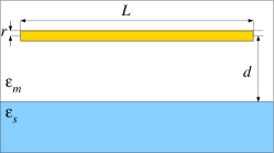
Figure 1: (Color online). Schematic view of the model considered: a finite-length nanowire immersed in the medium with the dielectric constant $\varepsilon_{m}$, interacting with the substrate with the dielectric constant $\varepsilon_{s}$.

For fixed boundary conditions $\varphi(0)=\varphi(L)=0$, $\Pi(0)=\Pi(L)=0$ the field operators can be expanded as follows:

$$\Big{(}\varphi(x),\Pi(x)\Big{)}=\sqrt{\frac{2}{L}}\sum_{n=1}^{N}\Big{(}\varphi_{n},\Pi_{n}\Big{)}\sin\frac{\pi nx}{L},$$ (3)

where it is implied that $n=0$ zero modes are absent in an open system, and the summation cutoff $N$ is about the number of elementary cells, $N\sim L/a$ ($a$ is the lattice constant that hereafter will be set to unity). After this expansion we have

$$\hat{H}_{LL}=\frac{\hbar v_{F}}{2}\sum_{n>0}\Big{\{}\Pi_{n}^{2}+\Big{(}\frac{\pi n}{L}\Big{)}^{2}\varphi_{n}^{2}\Big{\}},$$ (4)

and, after introducing the bosonic creation and annihilation operators $a_{n}^{{\dagger}},a_{n}$,

$$\varphi_{n}=\sqrt{\frac{L}{2\pi n}}(a_{n}^{{\dagger}}+a_{n}),\quad\Pi_{n}=i\sqrt{\frac{\pi n}{2L}}(a_{n}^{{\dagger}}-a_{n}),$$ (5)

the Luttinger liquid Hamiltonian (1) takes the familiar form

$$\hat{H}_{LL}=\frac{\pi\hbar v_{F}}{L}\sum_{n>0}n\Big{(}a_{n}^{{\dagger}}a_{n}+\frac{1}{2}\Big{)}.$$ (6)

It should be noted that fixed boundary conditions for $\varphi$ and $\Pi$ fields used above are not a standard way of implementing boundaries in a Luttinger liquid (requiring the electron wave function to vanish at the boundary results in a more complicated condition involving both $\varphi$ and $\Pi$); however, in the present work we are not interested in describing edge states or any other boundary phenomena. Our sole purpose is to take into account the finite size of the wire, and such simplified boundary conditions are fully sufficient for that purpose; previously, such an approach has been successfully used for studying the conductivity of finite chains Greschner+13 .

Including the contribution of the long-range Coulomb interactions between the electrons, we can write the full Hamiltonian as $\hat{H}=\hat{H}_{LL}+\hat{U}_{1}+\hat{U}_{2}$, where

$$\hat{U}_{1}=\frac{\varepsilon_{m}-\varepsilon_{s}}{8\pi\epsilon_{0}\varepsilon_{m}(\varepsilon_{m}+\varepsilon_{s})}\int_{0}^{L}\!\!dx\int_{0}^{L}\!\!dx^{\prime}\frac{\rho(x)\rho(x^{\prime})}{\sqrt{(x-x^{\prime})^{2}+(2d)^{2}}}$$ (7)

describes the interaction of electrons with the interface Jackson-book , and

$$\hat{U}_{2}=\frac{1}{8\pi\epsilon_{0}\varepsilon_{m}}\int_{0}^{L}\!\!dx\int_{0}^{L}\!\!dx^{\prime}\frac{\rho(x)\rho(x^{\prime})}{\sqrt{(x-x^{\prime})^{2}+(2r_{0})^{2}}}$$ (8)

corresponds to the direct Coulomb interaction between the electrons of the nanowire, regularized at small distances to avoid unphysical singularity. Expressions (7), (8) are written using the electrodynamic Green’s function in the non-retarded approximation, i.e., assuming that the typical wave length of electromagnetic fluctuations contributing to the interaction energy is much larger than $\max(L,d)$; we comment on the applicability limits of this approximation later.

The regularization length $r_{0}$ reflects the fact that the electron wave function in a nanowire is actually delocalized over some length which is about the wire diameter, and thus the singularity in the Coulomb interaction gets cured. The precise form of the wave function depends on the microscopic details of the confining potential, and thus the ”cutoff” is not exactly the wire diameter but a phenomenological quantity proportional to it. In what follows, for the sake of simplicity we set $r_{0}$ to the wire radius $r$; as we will see later, $r$ enters the results only via log corrections. This way of regularizing the Coulomb interaction in a nanowire has been introduced in Ref. GoldGhazali90, and is by now standard giamarchi-book .

We use a simplified model describing the substrate by a single parameter, dielectric constant, implicitly assumed to be frequency-independent. Although this model is certainly insufficient for a quantitative description, one can expect that it captures the essential physics of the vdW (non-retarded) regime, since the main contribution to the interaction energy in this regime comes from the range of relatively low frequencies where the dielectric constant of a typical covalent insulator weakly depends on the frequency.

The resulting Hamiltonian including interactions takes the following form:

$$\hat{H}=\frac{\pi\hbar v_{F}}{L}\sum_{nn^{\prime}}\Big{\{}T_{nn^{\prime}}\big{(}a^{{\dagger}}_{n}a_{n^{\prime}} + \frac{\delta_{nn^{\prime}}}{2}\big{)}$$

$$+ \frac{1}{2}\big{(}\Phi_{nn^{\prime}}a_{n}^{{\dagger}}a_{n^{\prime}}^{{\dagger}}+\text{h.c.}\big{)}\Big{\}},$$

where the matrix elements are given by

$$\Phi_{nn^{\prime}} = \frac{1}{2}\sqrt{nn^{\prime}}\big{[}b_{2}I_{nn^{\prime}}(s_{2})-b_{1}I_{nn^{\prime}}(s_{1})\big{]},$$

$$T_{nn^{\prime}} = n\delta_{nn^{\prime}}+\Phi_{nn^{\prime}},$$ (10)

and we have introduced the notation

$$I_{nn^{\prime}}(s)=\frac{1}{\pi^{2}}\int_{0}^{\pi}dt\int_{0}^{\pi}dt^{\prime}\;\frac{\cos(nt)\cos(nt^{\prime})}{\sqrt{(t-t^{\prime})^{2}+s^{2}}},$$ (11)

$$b_{1}=\frac{\varepsilon_{s}-\varepsilon_{m}}{\varepsilon_{s}+\varepsilon_{m}}b_{2},\quad b_{2}=\frac{2K\widetilde{\alpha}}{\pi\varepsilon_{m}},\quad\widetilde{\alpha}=\frac{e^{2}}{4\pi\epsilon_{0}\hbar v_{F}},$$

$$s_{1}=2\pi d/L,\quad s_{2}=2\pi r/L.$$ (12)

Here $\widetilde{\alpha}$ is the analog of the fine structure constant, with the speed of light $c$ replaced by the Fermi velocity $v_{F}$. Taking into account that typically $v_{F}\sim 10^{-2}c$, one concludes that typical values of $b_{1,2}$ are of the order of unity (or less if $\varepsilon_{m}$ is large). Properties of functions $I_{nn^{\prime}}(s)$ are listed in the Appendix.

The quadratic Hamiltonian (II) is readily diagonalized by the Bogoliubov transformation:

$$\hat{H}=\frac{\pi\hbar v_{F}}{L}\sum_{n>0}\lambda_{n}\big{(}A^{{\dagger}}_{n}A_{n}+\frac{1}{2}\big{)}$$ (13)

where $A_{n}$ are the unitary transformed bosonic operators, and $\lambda_{n}$ are positive solutions of the secular equation

$$\det(M-\lambda^{2}\openone)=0,\quad M=(T+\Phi)(T-\Phi).$$ (14)

Although $\lambda_{n}$ can be easily found numerically, below we demonstrate that a very good approximation is obtained by neglecting non-diagonal elements of $M$ altogether:

$$\lambda_{n}\approx\sqrt{M_{nn}}=n\big{[}1+b_{2}I_{nn}(s_{2})-b_{1}I_{nn}(s_{1})\big{]}^{1/2}.$$ (15)

This is explained by the fact that functions $I_{nn^{\prime}}(s)$ decay rather fast with $|n-n^{\prime}|$ (see the Appendix), so the ratio of non-diagonal to diagonal elements of $M$ is practically a small parameter, and the leading contribution to $\lambda_{n}$ from the non-diagonal part of $M$ comes in the second order in this small parameter.

III The vdW interaction potential

Having obtained the spectrum of the interacting Hamiltonian, we are now in a position to calculate the interaction potential as a function of the distance $d$ to the surface. At zero temperature, the vdW interaction energy $W(d)$ is simply the difference between the ground state energies taken at finite $d$ and at infinity:

$$W_{0}(d)=\frac{\pi\hbar v_{F}}{2L}\sum_{n}\big{(}\lambda_{n}-\lambda_{n}^{(0)}\big{)},\quad\lambda_{n}^{(0)}\equiv\lambda_{n}(d=\infty).$$ (16)

At finite temperature $T\not=0$ the vdW energy can be found as the corresponding difference of free energies, yielding

$$W(d) = W_{0}(d)+W_{T}(d),$$

$$W_{T}(d) = =T\sum_{n}\ln\left[\frac{1-e^{-{\ell_{T}\lambda_{n}}/{L}}}{1-e^{-{\ell_{T}\lambda_{n}^{(0)}}/{L}}}\right],$$ (17)

where

$$\ell_{T}=\pi\hbar v_{F}/T$$ (18)

is the characteristic thermal length.

In the pairwise additive approximation, the vdW interaction would always decay as $W(d)\propto d^{-3}$. The actual behavior of the interaction energy depends on the interplay of the four characteristic problem scales: the wire length $L$, distance to the surface $d$, the thermal length $\ell_{T}$, and the characteristic scale $\ell_{\Delta}$ related to the spectral gap (see Eq. 30 below). In all our calculations, we will assume that the distance to the surface is large compared to the wire radius, $d\gg r$.

III.1 The vdW interaction at $T=0$

Consider first the properties of the dispersive interaction energy at zero temperature. As shown below, those results will be applicable at finite temperatures as well, as long as $\ell_{T}\gg\min(d,L)$. In Fig. 2 we compare the results for the interaction energy obtained by exact numerical diagonalization of the matrix $M$ (see Eq. (14)) with those using the simple diagonal approximation (15): one can see that the diagonal approximation does a very good job, and we have checked this behavior for various ratios $L/r$. Thus, from now on we will adopt the diagonal approximation, assuming (15) for $\lambda_{n}$, and setting

$$\lambda_{n}^{(0)}\approx n\big{[}1+b_{2}I_{nn}(s_{2})\big{]}^{1/2}.$$ (19)

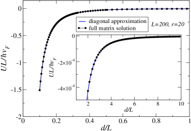
Figure 2: (Color online). Typical zero-temperature vdW interaction energy calculated via the full diagonalization of the matrix $M$ (14) (symbols), compared to the results of using the diagonal approximation (15). The parameters taken are $b_{1}=b_{2}=1$.

Asymptotic behavior of $W_{0}(d)$ can be easily analyzed in a few limiting cases. Since we assume $r\ll d$ and thus $s_{2}\ll s_{1}$, and $b_{1}$ and $b_{2}$ are of the same order of magnitude, it follows that $b_{1}I_{nn}(s_{1})\ll b_{2}I_{nn}(s_{2})$. Therefore, one may expand (15) in $b_{1}I_{nn}(s_{1})$, which yields

$$W_{0}(d)\approx-\frac{\pi\hbar v_{F}}{4L}\sum_{n>0}n\frac{b_{1}I_{nn}(s_{1})}{\sqrt{1+b_{2}I_{nn}(s_{2})}}.$$ (20)

This expression shows that the vdW energy, expressed in units of $\hbar v_{F}/L$ as a function of the dimensionless distance $d/L$, depends only on the geometric factor $L/r$ (at fixed $b_{1,2}$). This scaling is illustrated in Fig. 3.

III.1.1 $2\pi d\ll L$.

For $2\pi d\ll L$, the integrals $I_{nn}(s_{1,2})$ in Eq. (20) can be replaced by Macdonald’s functions (see Eq. (37)), so the summation is effectively cut off at $n\sim L/d$ (the summand decays exponentially for larger $n$). One can easily estimate the sum by passing to an integral; for $b_{2}\ln(d/r)\gg 1$ we obtain

$$\frac{W_{0}(d)}{L}\simeq-A\frac{b_{1}}{\sqrt{b_{2}}}\frac{\hbar v_{F}}{d^{2}\ln^{1/2}(\zeta d/r)},$$ (21)

where $A$ and $\zeta$ are some numbers of the order of unity. One can show that taking into account subleading terms in (37) yields merely a correction of the order of $d/L$ to (21).

It is easy to see from Eq. (20) that the main contribution to the interaction for $2\pi d\ll L$ is made by the modes with $2\pi nd/L\sim 1$, which corresponds to frequencies $\nu\sim v_{F}/2\pi d$ (e.g., for $d>10$ nm the relevant frequency range is $\nu\sim 10$ THz; in this region the dielectric constant of a typical covalent insulator should only weakly depend on the frequency). Thus, retardation effects remain negligible as long as the corresponding typical electromagnetic wave length $2\pi d(c/v_{F})$ remains large compared to $L$. This determines the range of distances where the non-retarded vdW regime is realized, $L(v_{F}/c)\ll 2\pi d\ll L$.

For $b_{2}\ln(d/r)\ll 1$ (since the “fine structure constant” $\tilde{\alpha}\sim 1$, this regime might be realized only if $\varepsilon_{m}\gg 1$) the term involving $b_{2}$ in (20) can be neglected, and the result is

$$\frac{W_{0}(d)}{L}\simeq\widetilde{A}b_{1}\frac{\hbar v_{F}}{d^{2}},$$ (22)

where $\widetilde{A}\sim 1$ is another numerical factor.

III.1.2 $2\pi d\gg L$.

In this case, $I_{nn}(s_{1})$ in Eq. (20) can be replaced by its asymptotics $4/(\pi n^{4}s_{1}^{3})$, see Eq. (36), which yields the standard $1/d^{3}$ behavior for the vdW energy:

$$\frac{W_{0}(d)}{L}\simeq-\frac{b_{1}}{8\pi^{3}}f\Big{(}b_{2},\frac{r}{L}\Big{)}\frac{L\hbar v_{F}}{d^{3}}.$$ (23)

Here the function $f(b_{2},r/L)$, defined as

$$f\Big{(}b_{2},\frac{r}{L}\Big{)}=\sum_{n\geq 1}\frac{1}{n^{3}}\frac{1}{\sqrt{1+b_{2}K_{0}(2\pi nr/L)}},$$ (24)

weakly depends on its arguments, being always a number of the order of unity (see Fig. 4).

As seen from the above formula, for $2\pi d\gg L$ the main contribution to the interaction energy comes from the modes with low frequencies $\nu\lesssim v_{F}/L$, so the non-retarded approximation remains valid if the typical electromagnetic wave length $L(c/v_{F})$ is large compared to $d$. Thus, non-retarded regime is in this case realized in the distance range $L/(2\pi)\ll d\ll(c/v_{F})L$.

A comparison of Eqs. (23) and (21) shows that the vdW power law changes from $W\sim d^{-3}$ at large distances $d\gg L$ to $W\sim d^{-2}/\ln(d/r)$ at small distances $d\ll L$.

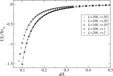
Figure 3: Zero-temperature vdW interaction energy at $b_{1}=b_{2}=1$, expressed in units of $\hbar v_{F}/L$ as a function of the dimensionless distance $d/L$, for several values of the nanowire length $L$ and radius $r$, with the elongation factor $L/r$ is kept fixed.

III.2 Finite temperature effects

The summation in (III) is effectively cut off at $n\sim n_{T}=L/\ell_{T}$, so the thermal contribution $W_{T}(d)$ to the vdW energy is exponentially small if $\ell_{T}\gg L$. We therefore assume that the opposite condition of high temperatures $\ell_{T}\ll L$ is satisfied, which renders the contribution of thermal fluctuations into the form

$$W_{T}\simeq-T\sum_{n=1}^{n_{T}}\ln\frac{\lambda_{n}^{(0)}}{\lambda_{n}}.$$ (25)

Expanding in $b_{1}I_{nn}(s_{1})$ as done before for $T=0$ case, one can obtain an estimate for the thermal contribution in the following form which is easy to analyze:

$$W_{T}(d)\simeq-\frac{T}{2}\sum_{n=1}^{n_{T}}\frac{b_{1}I_{nn}(s_{1})}{1+b_{2}I_{nn}(s_{2})}.$$ (26)

Below we will see that the thermal contribution dominates over the quantum one when $\ell_{T}\ll\min(d,L)$.

III.2.1 $2\pi d\ll L$.

For $d\ll\ell_{T}\ll L$, the thermal contribution is roughly a factor $(d/\ell_{T})^{2}$ smaller than the quantum one (21), and thus can be neglected. For $\ell_{T}\ll d\ll L$, the estimate yields

$$\frac{W_{T}(d)}{L}\simeq\begin{cases}\displaystyle-B\left(\frac{\varepsilon_{s}-\varepsilon_{m}}{\varepsilon_{s}+\varepsilon_{m}}\right)\frac{T}{d\ln(\kappa d/r)},&b_{2}\ln(d/r)\gg 1\\ \displaystyle-\widetilde{B}b_{1}(T/d),&b_{2}\ln(d/r)\ll 1\end{cases},$$ (27)

where $B$, $\widetilde{B}$, and $\kappa$ are numerical factors $~{}1$. It is easy to see that in this regime the contribution of thermal fluctuations is much larger than the corresponding contribution of the ground state energy (21), (22). The condition of applicability of non-retarded approximation remains the same as in the $T=0$ case, namely $L(v_{F}/c)\ll 2\pi d\ll L$.

It is interesting to note that in the retarded regime $L\to\infty$ Emig et al. Emig+06 obtained an expression for the interaction energy that is similar to the first line of Eq. (27) but has a different logarithmic factor ($\ln(c\ell_{T}/v_{F}r)$ instead of $\ln(d/r)$).

III.2.2 $2\pi d\gg L$.

If $L\ll\ell_{T}\ll d$, the thermal contribution is negligible as discussed above, so the only regime where thermal fluctuations dominate the vdW energy is $\ell_{T}\ll L\ll d$:

$$\frac{W_{T}(d)}{L}\simeq-\frac{b_{1}}{4\pi^{4}}\frac{TL^{2}}{d^{3}}g(b_{2},r/L),\quad\ell_{T}\ll L\ll d.$$ (28)

Here function $g(b_{2},r/L)$ is defined as follows:

$$g\Big{(}b_{2},\frac{r}{L}\Big{)}=\sum_{n\geq 1}\frac{1}{n^{4}}\frac{1}{1+b_{2}K_{0}(2\pi nr/L)},$$ (29)

and is presented in Fig. 4 for a few fixed values of $L/r$. Again, the condition of applicability of non-retarded approximation remains the same as in the $d\gg L$ case at $T=0$, namely $L/(2\pi)\ll d\ll(c/v_{F})L$.

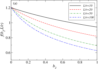
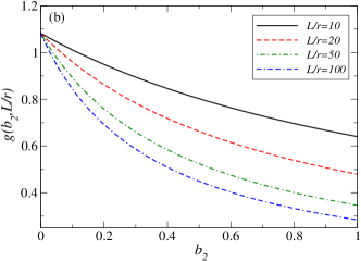
Figure 4: (Color online). Plots of scaling functions $f(b_{2})$ and $g(b_{2})$, defined by Eqs. (24) and (29), respectively, for several values of the elongation factor $L/r$.

III.3 Effects of a finite spectral gap

Although our formalism is based on bosonization and therefore is tuned to metallic nanowires, it is easy to incorporate effects of a small spectral gap $\Delta$ and thus generalize our calculations to the case of narrow-gap semiconducting wires. Indeed, to introduce a gap, one has to add the “mass term”

$$\frac{1}{2}\hbar v_{F}\int dx\,(\Delta/\hbar v_{F})^{2}\varphi^{2}$$

to the Hamiltonian (1). Then, in Eqs. (4), (5), and (6) one has to make the replacement $n\mapsto\sqrt{n^{2}+n_{\Delta}^{2}}$, where

$$\ell_{\Delta}=\frac{\pi\hbar v_{F}}{\Delta},\quad n_{\Delta}=\frac{L}{\ell_{\Delta}},$$ (30)

$\ell_{\Delta}$ being a new characteristic length scale related to the gap. The full Hamiltonian keeps the form (II), with the amplitudes modified as follows:

$$\Phi_{nn^{\prime}} = \frac{1}{2}\frac{nn^{\prime}\big{[}b_{2}I_{nn^{\prime}}(s_{2})-b_{1}I_{nn^{\prime}}(s_{1})\big{]}}{[(n^{2}+n_{\Delta}^{2})(n^{\prime 2}+n_{\Delta}^{2})]^{1/4}},$$

$$T_{nn^{\prime}} = \sqrt{n^{2}+n_{\Delta}^{2}}\delta_{nn^{\prime}}+\Phi_{nn^{\prime}}.$$ (31)

The diagonal approximation (15) for $\lambda_{n}$ gets modified accordingly:

$$\lambda_{n}\simeq\big{\{}n_{\Delta}^{2}+n^{2}\big{[}1+b_{2}I_{nn}(s_{2})-b_{1}I_{nn}(s_{1})\big{]}\big{\}}^{1/2}.$$ (32)

Our analysis shows (see Fig. 5) that the effect of a finite gap becomes dominating if the condition $\ell_{\Delta}\ll\min(d,L)$ is satisfied, and in this case the behavior of the vdW interaction energy is governed by the standard power law (as given by the pairwise additive approximation) $W(d)\propto d^{-3}$. Thus, introduction of a spectral gap (i.e., making the wire insulating) leads to the same power law exponent that corresponds to large distances $d\gg L$. It should be noted that this effect is similar to that obtained by Dobson et al. Dobson+06 for two parallel wires, where the behavior of the vdW energy changed from $W\sim d^{-5}$ for insulating wires to $W\sim d^{-2}/\ln^{3/2}(d/r)$ for metallic ones (in fact, the latter expression has been obtained much earlier by other authors Chang+71 ; Glasser72 ).

IV Discussion and summary

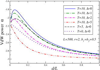
Figure 5: (Color online). Behavior of the vdW power law exponent defined by Eq. (33) as a function of the wire-surface separation $d$, for different values of the temperature $T$ and the spectral gap $\Delta$ expressed in the units of $\hbar v_{F}/L$. Non-monotonic behavior of $\alpha$ is suppressed with the increase of the gap.

The analytical estimates obtained in the previous section suggest that if one describes the vdW interaction between a wire and a surface by means of a power law $W(d)\propto d^{\alpha}$, then the “running exponent”

$$\alpha=\frac{\partial\ln W}{\partial\ln d}$$ (33)

is a complicated function of the distance $d$. For instance, at $T=0$ the asymptotics (21), (23) show that this exponent must monotonically change from $\alpha=-3$ at large distances $d\gg L$ to $\alpha=-2$ at small distances $d\ll L$. If temperature is high enough to make $\ell_{T}\ll L$, according to Eqs. (27), (28) the behavior of $\alpha$ should be non-monotonic, changing from $\alpha=-3$ at $d\gg L$, to $\alpha=-1$ at $\ell_{T}\ll d\ll L$ and back to $\alpha=-2$ at $d\ll\ell_{T}$.

This is indeed demonstrated in Fig. 5, where we present the results of numerical calculations using Eqs. (16), (III) in the diagonal approximation for $\lambda_{n}$. One can see that an increase of the spectral gap leads to a rapid suppression of “unconventional” power laws, squeezing the corresponding range of distances. This is in line with the general idea that unconventional power laws stem from delocalized excitations Dobson+06 ; Ambrosetti+16 , while the presence of a gap introduces a finite correlation length. Further, one can see that a non-monotonic behavior of $\alpha$ as a function of $d$ is observed only as long as the gap is sufficiently small, so that $\ell_{\Delta}\gg\ell_{T}$.

The “conventional” $1/d^{3}$ dependence of the vdW interaction energy can be understood as the result of pairwise summation of the standard $1/d^{6}$ potential of vdW interaction between the elements of the wire and surface viewed as point-like particles. This result is valid for a gapped wire if the gap is larger than $\hbar\pi v_{F}/\min(L,d)$. For a wire with smaller gap, as we have shown, this pairwise additive result is correct only if the wire is far enough from the surface to be itself approximately considered as a point-like object (practically if $d>L$). For shorter distances $d<L$ the gapless and delocalized character of nanowire excitations becomes important (the essential point is that the wire susceptibility has strong dependence both on the frequency and the wave vectorDobson+06 ; Ambrosetti+16 ), and as the result the power law exponent $\alpha$ changes from $-3$ to “nearly $-2$” or “nearly $-1$” (“nearly” meaning the presence of log corrections), respectively to whether the energetic or enthropic contribution is dominating. Since the energetic contribution always wins at distances $d$ smaller that the characteristic thermal length $\ell_{T}$, for finite temperature there are three distinct regimes of $\alpha$ going from $-3$ to $-1$ and back to $-2$ with the decreasing distance $d$. Generally, for $d<L$ there are logarithmic corrections to the power law which stem from the Coulomb interaction between electrons inside the nanowire. Those log corrections may become negligible if the parameter $b_{2}$ is small enough; however, since the “fine structure constant” $\tilde{\alpha}\sim 1$, this regime might be realized only if the dielectric constant of the medium is large, $\varepsilon_{m}\gg 1$.

It should be remarked that a non-monotonic behavior of the vdW power law exponent has been observed in the many-body dispersion (MBD) calculation Ambrosetti+16 for the vdW interaction between two parallel carbyne wires. However, the origin of such a behavior is different from our case since the calculation in Ref. Ambrosetti+16, has been performed for $T=0$; in their results, non-monotonicity reveals itself only at extremely small distances $d/L\lesssim 10^{-2}$ and is probably connected with details of the specific realization of the MBD model. In our case, non-monotonicity is the effect of finite temperature which sets in at distances $d/L\sim 0.1$.

To summarize, we have applied the Luttinger liquid approach to study the vdW interaction between a finite-size metallic or narrow-gap semiconductor nanowire and an insulating or perfect-metal surface. We focused on the case of a strongly one-dimensional wire, such as a carbon nanotube or a single polymer molecule, which is not correctly described by the Fermi liquid. We obtained simple analytical expressions describing the vdW interaction in different regimes determined by the interplay between characteristic length scales set by the spectral gap and temperature, the nanowire length, and the wire-surface distance. It is shown that the effective vdW power law exponent is generally a complicated function of wire-surface distance, which can be non-monotonic if the gap is small enough compared to the temperature.

It should be emphasized that our results are obtained in the previously unexplored non-retarded regime that is realized at intermediate wire-surface distances

$$(v_{F}/c)L\ll d\ll L\quad\text{or}\quad L\ll d\ll(c/v_{F})L,$$ (34)

where $v_{F}\sim 10^{-2}c$ is the characteristic velocity of nanowire electrons (for a metallic wire, it is the Fermi velocity). For that reason, they cannot be directly related to the results of previous studies Emig+06 ; Bordag+06 ; Bordag06 ; Noruzifar+11 ; Noruzifar+12 since those were obtained for the model of an infinitely long wire ($L\to\infty$). It is interesting to note that in the $d\ll L$ case our $T=0$ result (21) for the interaction energy has the same functional dependence on the distance $d$ as the retarded-regime expression obtained by Noruzifar et al. Noruzifar+11 ; Noruzifar+12 for a ”plasma cylinder” interacting with a perfect metal plate; however, those two results correspond to different physics, as is obvious from the fact that the prefactor in the result of Noruzifar et al. vanishes when the cylinder radius goes to zero, while in our case the prefactor contains the Fermi velocity and does not depend on the wire radius.

There are further similarities between our results and those obtained previously in the retarded regime. For example, in the “universal” limit $d/r\to\infty$, $L=\infty$ the dispersive interaction energy is Emig+06 ; Noruzifar+11 $W=-\hbar cL/[16\pi d^{2}\ln(d/r)]$, which is “nearly $\alpha=-2$” power law as our Eq. (21), but contains $c$ instead of $v_{F}$ and has a different power in the logarithmic correction. In the high-temperature retarded regime Emig et al. Emig+06 obtained an expression for the interaction energy which is similar to the first line of Eq. (27) but again has a different logarithmic factor, $\ln(c\ell_{T}/v_{F}r)$ instead of $\ln(d/r)$. Although the underlying physics, as we emphasized before, is different, those similarities in functional dependence of the interaction energy on distance stem from the analogous mathematical structure of summing over gapless modes with linear quasi-1d dispersion: in our case those modes are plasmons, in the retarded regime they are electromagnetic waves. The origin of log corrections in the retarded regime is different as well: they arise due to the logarithmic behavior of the 1d propagator in the limit of low wave vectors.

Finally, we would like to remark on the origin of similarities between our results, obtained by the direct microscopic description of the wire in the bosonization framework, and those of Dobson et al. Dobson+06 who studied interaction between two parallel infinite-length wires using RPA expressions for the wire response: (i) in one dimension, as it is well known DzyaloshinskiiLarkin73 , RPA gives essentially exact results for the density-density correlation function, which are the same as in the Luttinger liquid approach giamarchi-book , and (ii) obviously the interaction between two wires is sufficiently similar to the interaction between a wire and its “mirror image” below the surface (which is what the non-retarded approximation essentially reduces to). We have checked that results of Ref. Dobson+06, are reproduced in the approach of two interacting Luttinger liquids (with the additional bonus of the ability to consider finite-length wires), but this is outside the scope of the present work.

Appendix: Properties of $I_{nn^{\prime}}(s)$

Here we list some properties of functions $I_{nn^{\prime}}(s)$ defined in (11). Passing from $y$, $y^{\prime}$ to new variables $y\pm y^{\prime}$, one can perform one integration and rewrite the integral as

$$I_{nn^{\prime}}(s)=\begin{cases}0,&|n-n^{\prime}|=\text{odd}\\ \displaystyle-\frac{2}{\pi(n^{2}-n^{\prime 2})}\int_{0}^{\pi/s}dz\frac{n\sin(nsz)-n^{\prime}\sin(n^{\prime}sz)}{\sqrt{1+z^{2}}},&n\not=n^{\prime}\\ \displaystyle\frac{1}{\pi n}\int_{0}^{\pi/s}dz\frac{n(\pi-sz)\cos(nsz)-\sin(nsz)}{\sqrt{1+z^{2}}},&n=n^{\prime}.\end{cases}$$ (35)

The asymptotic expressions for small and large argument are easily obtained. For $s\gg 1$ the leading asymptotics are

$$I_{nn^{\prime}}(s)\approx\begin{cases}\displaystyle\frac{6\pi}{n^{2}n^{\prime 2}s^{5}}+O(s^{-7}),&\text{$n$ and $n^{\prime}$ are even}\\ \displaystyle\frac{4}{\pi n^{2}n^{\prime 2}s^{3}}+O(s^{-5}),&\text{$n$ and $n^{\prime}$ are odd}\end{cases},$$ (36)

and for $s\ll 1$ one has

$$I_{nn^{\prime}}(s)\approx\begin{cases}\displaystyle-\frac{1}{n+n^{\prime}}+\frac{2s}{\pi}+O(s^{2}),&\text{$n\not=n^{\prime}$}\\ \displaystyle K_{0}(ns)-\frac{\text{Si}(\pi n)}{\pi n}+O(s^{2}),&\text{$n=n^{\prime}$,}\end{cases}$$ (37)

where $K_{0}(z)$ is the modified Bessel function of the second kind (the Macdonald function), and $\text{Si}(z)$ is the sine integral function.

References

- (1) L. M. Woods, D. A. R. Dalvit, A. Tkatchenko, P. Rodriguez-Lopez, A. W. Rodriguez, and R. Podgornik, Rev. Mod. Phys. 88, 045003 (2016)
- (2) V. Adrian Parsegian, Van Der Waals Forces: A Handbook For Biologists, Chemists, Engineers, And Physicists (Cambridge University Press, Cambridge, New York 2006).
- (3) D. Dalvit, P. Milonni, D. Roberts, F. da Rosa (Eds), Casimir Physics, Lecture Notes in Physics 834 (Springer, Berlin 2011).
- (4) A. Tkatchenko, Adv. Funct. Mater. 25, 2054 (2015).
- (5) A. M. Reilly and A. Tkatchenko, Chem. Sci. 6, 3289 (2015).
- (6) A. Ambrosetti, N. Ferri, R. A. DiStasio Jr., A. Tkatchenko, Science 351, 1171 (2016).
- (7) J. K. Norskov, T. Bligaard, J. Rossmeisl, and C. H. Christensen, Nature Chem. 1, 37 (2009).
- (8) K. Moth-Poulsen and T. Bjornholm, Nature Nanotech. 4, 551 (2009).
- (9) L. Bartels, Nature Chem. 2, 87 (2010).
- (10) G. Singh, H. Chan, A. Baskin, E. Gelman, N. Repnin, P. Král, and R. Klajn, Science 345, 1149 (2014).
- (11) D.B. Chang, R.L. Cooper, J.E. Drummond, and A.C. Young, Phys. Lett. 37A, 311 (1971).
- (12) M.L. Glasser, Phys. Lett. 42A, 41 (1972).
- (13) J. F. Dobson, A. White, A. Rubio, Phys. Rev. Lett. 96, 073201 (2006).
- (14) A. J. Misquitta, J. Spencer, A. J. Stone, A. Alavi, Phys. Rev. B 82, 075312 (2010).
- (15) A. J. Misquitta, R. Maezono, N. D. Drummond, A. J. Stone, R. J. Needs, Phys. Rev. B 89, 045140 (2014).
- (16) J. F. Dobson, T. Gould, G. Vignale, Phys. Rev. X 4, 021040 (2014).
- (17) A. Tkatchenko, R. A. DiStasio Jr., R. Car, M. Scheffler, Phys. Rev. Lett. 108, 236402 (2012).
- (18) T. Emig, R. L. Jaffe, M. Kardar, and A. Scardicchio, Phys. Rev. Lett. 96, 080403 (2006).
- (19) M. Bordag, B. Geyer, G. L. Klimchitskaya, and V. M. Mostepanenko, Phys. Rev. B 74, 205431 (2006).
- (20) M. Bordag, Phys. Rev. D 73, 125018 (2006).
- (21) E. Noruzifar, T. Emig, and R. Zandi, Phys. Rev. A 84, 042501 (2011).
- (22) E. Noruzifar, T. Emig, U. Mohideen, and R. Zandi, Phys. Rev. B 86, 115449 (2012).
- (23) In this case, there are always regions of the wire and of the surface separated by a sufficiently large distance such that the characteristic propagation time is larger than the typical period of local charge density oscillations, so retardation should be taken into account.
- (24) T. Giamarchi, Quantum Physics in One Dimension (Oxford University Press, Oxford, 2003).
- (25) S. Greschner, A. K. Kolezhuk, and T. Vekua, Phys. Rev. B 88, 195101 (2013).
- (26) J. D. Jackson, Classical Electrodynamics, 3rd ed. (Wiley, 1998).
- (27) A Gold and A. Ghazali, Phys. Rev. B 41, 7626 (1990).
- (28) I. E. Dzyaloshinskii and A. I. Larkin, Zh. Eksp. Teor. Fiz. 65, 411 (1973) [Sov. Phys. JETP 38, 202 (1974)].