Abstract

Brain plasticity, also known as neuroplasticity, is a fundamental mechanism of neuronal adaptation in response to changes in the environment or due to brain injury. In this review, we show our results about the effects of synaptic plasticity on neuronal networks composed by Hodgkin-Huxley neurons. We show that the final topology of the evolved network depends crucially on the ratio between the strengths of the inhibitory and excitatory synapses. Excitation of the same order of inhibition revels an evolved network that presents the rich-club phenomenon, well known to exist in the brain. For initial networks with considerably larger inhibitory strengths, we observe the emergence of a complex evolved topology, where neurons sparsely connected to other neurons, also a typical topology of the brain. The presence of noise enhances the strength of both types of synapses, but if the initial network has synapses of both natures with similar strengths. Finally, we show how the synchronous behaviour of the evolved network will reflect its evolved topology.

1 Introduction

The brain is the most complex organ in the human body. It contains approximately $10^{2}$ billion neurons and $10^{3}$ trillion synaptic connections, where each neuron can be connected to up to $10^{4}$ other neurons [1]. The neuron is the basic working unit of the brain and it is responsible for carrying out the communication and the processing of information within the brain [2]. Those tasks are achieved through neuronal firing spatio-temporal patterns that are depended on the neuron own dynamics and the way they are networked.

Towards the goal to understand the brain, over the past several years, mathematical models have been introduced to emulate neuronal firing patterns. A simple model that has been considered to describe neuronal spiking is based on the cellular automaton [3, 4]. This model uses discrete state variables, coordinates and time [5]. Another proposed bursting behaviour model is a simplification of the neuron model described by differential equations, where the state variables are continuous, while the coordinates and the time are discrete [6, 7, 8]. Recently, Girardi-Schappo et al. [9] proposed a map that reproduces neuronal excitatory and autonomous behaviour that are observed experimentally.

Differential equations have also been used to model neuronal patterns [10, 11, 12]. The integrate-and-fire model was developed by Lapicque in 1907 [13] and it is still widely used. But one of the most successful and cerebrated mathematical models using differential equations was proposed by Hodgkin and Huxley in $1952$ [14]. The Hodgkin-Huxley model explains the ionic mechanisms related to propagation and initiation of action potentials, i.e., the characteristic potential pulse that propagates in the neurons. In $1984$, Hindmarsh and Rose [15] developed a model that simulates bursts of spikes. The phenomenological Hindmarsh-Rose model may be seen as a simplification of the Hodgkin-Huxley model.

Hodgkin-Huxley neuron networks have been successfully used as a mathematical model to describe processes occurring in the brain. An important brain activity phenomenon is the neuronal synchronisation. This phenomenon is related to cognitive functions, memory processes, perceptual and motor skills, and information transfer [12, 16, 17, 18, 19].

There has been much work on neuronal synchronisation. Temporal synchronisation of neuronal activity happens when neurons are excited synchronously, namely assemblies of neurons fire simultaneously [12, 20]. Newly, Borges and collaborators [21] modelled spiking and bursting synchronous behaviour in a neuronal network. They showed that not only synchronisation, but also the kind of synchronous behaviour depends on the coupling strength and neuronal network connectivity. Studies showed that phase synchronisation is related to information transfer between brain areas at different frequency bands [22]. Neuronal synchronisation can be related to brain disorders, such as epilepsy and Parkinson’s disease. Parkinson’s disease is associated with synchronised oscillatory activity in some specific part of the brain [23]. Based on that, Lameu et al. [24] proposed interventions in neuronal networks to provide a procedure to suppress pathological rhythms associated with forms of synchronisation.

In this review, we focus the attention on the weakly and strongly synchronous states in dependence with brain plasticity. Brain plasticity, also known as neuroplasticity, is a fundamental mechanism for neuronal adaptation in response to changes in the environment or to new situations [25]. In 1890, James [26] proposed that the interconnection among the neurons in the brain and so the functional behaviour carried on by neurons are not static. Experimental evidence of plasticity was demonstrated by Lashley in 1923 [27] through experiments on monkeys. Scientific evidence of anatomical brain plasticity was published in 1964 by Bennett et al. [28] and Diamond et al. [29].

In the field of theoretical neuroscience, Hebb [30] wrote his ideas in words that inspired mathematical modelling related to synaptic plasticity [31]. According to Hebbian theory, the synaptic strength increases when a presynaptic neuron participates in the firing of a postsynaptic neuron, in other words, neurons that fire together, also wire together. The Hebbian plasticity led to the modelling of spike timing-dependent plasticity (STDP) [32, 33]. It was possible to obtain the STDP function for excitatory synapses by means of synaptic plasticity experiments performed by Bi and Poo [34]. The STDP function for inhibitory synapses was reported in experimental results in the entorthinal cortex by Haas et al. [35].

In this review, we show results that allow to understand the relation between spike synchronisation and synaptic plasticity and this dependence with the non-trivial topology that is induced in the brain due to STDP. As so, we consider an initial all-to-all network, where the neuronal network is built by connecting neurons by means of excitatory and inhibitory synapses. We show that the transition from weakly synchronous to strongly synchronous states depends on the neuronal network architecture, as well as to the STDP network evolves to non-trivial topology. When the strength of the inhibitory connections is of the same order of that of the excitatory connections, the final topology in the plastic brain presents the rich-club phenomenon, where neurons that have high degree connectivity towards neurons of the same presynaptical group (either excitatory of inhibitory) become strongly connected to neurons of the other postsynaptical group. The final topology has all the features of a non-trivial topology, when the strength of the synapses becomes reasonably larger than the strength of the excitatory connections, where neurons only sparsely connect to other neurons.

The structure of the review is the following. In Section $2$, we introduce the Hodgkin-Huxley model for a neuron and the synchronisation dynamics of neuronal networks. Section $3$ presents the Hebbian rule and the spike-timing dependent plasticity (STDP) in excitatory and inhibitory synapses. In Section $4$, we show the effects of the synaptic plasticity on the network topology and synchronous behaviour. Finally, in the last Section, we draw the conclusions.

2 Hodgkin-Huxley Neuronal Networks

2.1 Neurons

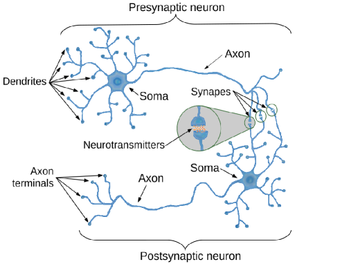
Figure 1: Schematic illustration showing the three main parts of neurons (dendrite, soma and axon), including the presynaptic and postsynaptic neurons.

Neurons are cells responsible for receiving, processing and transmitting information in the neuronal system [36]. They have differences in sizes, length of axons and dendrites, in the number of dendrites and axons terminals. Figure 1 illustrates the three main parts of the neuron: dendrite, cell body or soma, and axon [37]. The dendrites are responsible for the signal reception, and the axons drive the impulse from the cell body to another neuron. The neurons are connected through synapses, where the neuron that sends the signal is called presynaptic and the postsynaptic is the neuron that receives it. The most common form of neuron communication is by means of the chemical synapses, where the signal is propagated from the presynaptic to postsynaptic neurons by releasing neurotransmitters.

The signal propagates by means of the variation of internal neuron electric potential. An action potential occurs when a neuron sends information from the soma to the axon. The action potential is characterised by a rapid change in the membrane potential, as shown in Fig. 2. In the absence of stimulus, the membrane potential remains near a baseline level. A depolarisation occurs when the action potential is greater than a threshold value. After the depolarisation, the action potential goes through a certain repolarisation stage, where the action potential rapidly reaches the refractory period or hyperpolarisation. The refractory period is the time interval in which the axon does not transmit the impulse [37].

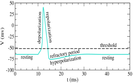
Figure 2: Plot of the action potential showing the various phases at a point on the cell membrane.

Action potentials are generated and propagates due to different ions crossing the neuron membrane. The ions can cross the membrane through ion channels and ion pumps [38]. Figure 3(a) shows the ion channels of sodium (${\rm Na}^{+}$) and potassium (${\rm K}^{+}$). In the depolarisation stage, a great amount of sodium ions move into the axon (I), while the repolarisation occurs when the potassium ions move out of the axon (II). Figure 3(b) shows the transport of sodium (I and II) and potassium ions (III and IV) through the pumps. The sodium-potassium pumps transport sodium ions out and potassium ions in, and it is responsible for maintaining the resting potential [38].

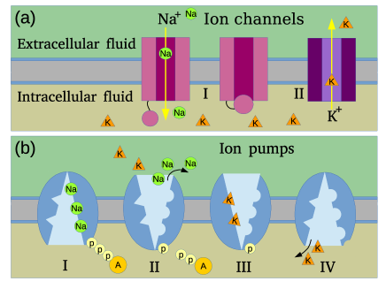
Figure 3: Schematic diagram of the ions traffic across cell membranes, (a) ion channels and (b) ion pumps.

2.2 Hodgkin-Huxley Model

Hodgkin and Huxley [14] performed experiments on the giant squid axon using microelectrodes introduced into the intracellular medium. They proposed a mathematical model that allowed the development of a quantitative approximation to understand the biophysical mechanism of action potential generation. In 1963, Hodgkin and Huxley were awarded with the Nobel Prize in Physiology or Medicine for their work. The Hodgkin-Huxley model is given by

$$C\dot{V} = I-g_{\rm K}n^{4}(V-E_{\rm K})-g_{\rm Na}m^{3}h(V-E_{\rm Na})-g_{L}(V-E_{\rm L}),$$

$$\dot{n} = \alpha_{n}(V)(1-n)-\beta_{n}(V)n,$$ (1)

$$\dot{m} = \alpha_{m}(V)(1-m)-\beta_{m}(V)m,$$ (2)

$$\dot{h} = \alpha_{h}(V)(1-h)-\beta_{h}(V)h,$$ (3)

where $C$ is the membrane capacitance ($\mu$F/cm²), $V$ is the membrane potential (mV), $I$ is the constant current density, parameter $g$ is the conductance, and $E$ the reversal potentials for each ion. The functions $m(V)$ and $n(V)$ represent the activation for sodium and potassium, respectively, and $h(V)$ is the function for the inactivation of sodium. The functions $\alpha_{n}$, $\beta_{n}$, $\alpha_{m}$, $\beta_{m}$, $\alpha_{h}$, $\beta_{n}$ are given by

$$\alpha_{n}(v) = \frac{0.01v+0.55}{1-\exp\left(-0.1v-5.5\right)},$$ (4)

$$\beta_{n}(v) = 0.125\exp\left(\frac{-v-65}{80}\right),$$ (5)

$$\alpha_{m}(v) = \frac{0.1v+4}{1-\exp\left(-0.1v-4\right)},$$ (6)

$$\beta_{m}(v) = 4\exp\left(\frac{-v-65}{18}\right),$$ (7)

$$\alpha_{h}(v) = 0.07\exp\left(\frac{-v-65}{20}\right),$$ (8)

$$\beta_{h}(v) = \frac{1}{1+\exp\left(-0.1v-3.5\right)},$$ (9)

where $v=V/$[mV]. We consider $C=1$ $\mu$F/cm², $g_{\rm K}=36$mS/cm², $E_{\rm K}=-77$mV, $g_{\rm Na}=120$mS/cm², $E_{\rm Na}=50$mV, $g_{\rm L}=0.3$mS/cm², $E_{\rm L}=-54.4$mV [21]. Depending on the value of the external current density $I$ ($\mu$A/cm²) the neuron can present periodic spikings or single spike activity. In the case of periodic spikes, if the constant $I$ increases, the spiking frequency also increases. Figure 4 shows the temporal evolution of the membrane potential of a Hodgkin-Huxley neuron for $I=0\mu$A/cm² (black line) and for $I=9\mu$A/cm² (red line). For the case without current, the neuron shows an initial firing and, after the spike, it remains in the resting potential. In the second case the external current $I$ is greater than the required threshold and the neuron exhibits firings.

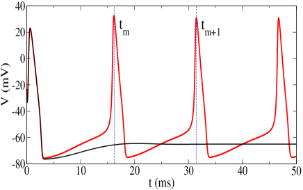
Figure 4: Membrane potential $V$ of a Hodgkin-Huxley neuron with $I=0\mu$A/cm² (black line) and $I=9\mu$A/cm² (red line).

2.3 Neuronal Synchronisation

The synchronisation process here is related to natural phenomena ranging from metabolic processes in our cells to the highest cognitive activities [39]. Neuronal synchronisation has been found in the brain during different tasks and at rest [40]. We study in this text neuronal synchronisation process in a network of coupled Hodgkin-Huxley neurons. The network dynamics is given by [41]

$$C\dot{V_{\rm i}} = I_{\rm i}-g_{\rm K}n^{4}(V_{\rm i}-E_{\rm K})-g_{\rm Na}m^{3}h(V_{\rm i}-E_{\rm Na})$$ (10)

$$-g_{L}(V_{\rm i}-E_{\rm L})+\frac{(V_{\rm r}^{\rm Exc}-V_{\rm i})}{\omega_{\rm Exc}}\sum_{j=1}^{N_{\rm Exc}}\varepsilon_{\rm ij}s_{\rm j}$$

$$+\frac{(V_{r}^{\rm Inhib}-V_{\rm i})}{\omega_{\rm Inhib}}\sum_{j=1}^{N_{\rm Inhib}}\sigma_{\rm ij}s_{\rm j}+\Gamma_{i},$$

where the elements of the matrix $\varepsilon_{\rm ij}$ ($\sigma_{\rm ij}$) are the intensity of the excitatory (inhibitory) synapse (coupling strength) between the presynaptic neuron $j$ and the postsynaptic neuron $i$, $\omega_{\rm Exc}$ ($\omega_{\rm Inhib}$) represents the mean number of excitatory (inhibitory) synapses of each neuron, $\Gamma_{i}$ is an external perturbation so that the neuron is randomly chosen and the chosen one receives an input with a constant intensity $\gamma$, $N_{\rm Exc}$ is the number of excitatory neurons, and $N_{\rm Inhib}$ is the number of inhibitory neurons. The excitatory (inhibitory)neurons are connected with reverse potential $V_{\rm r}^{\rm Exc}=20\rm mV$ ($V_{\rm r}^{\rm Inhib}=-75\rm mV$), and the postsynaptic potential $s_{i}$ is given by [41]

$$\frac{ds_{i}}{dt}=\frac{5(1-s_{i})}{1+\exp(-\frac{V_{i}+3}{8})}-s_{i}.$$ (11)

One measure that we adopt to quantify synchronous behaviour is the Kuramoto order parameter that reads as [42]

$$Z(t)=R(t){\rm e}^{i\psi(t)}=\frac{1}{N}\sum_{j=1}^{N}{\rm e}^{i\theta_{j}(t)},$$ (12)

where $R(t)$ is the amplitude, $\psi(t)$ is the angle of a centroid phase vector, and

$$\theta_{j}(t)=2\pi\frac{t-t_{j,m}}{t_{j,m+1}-t_{j,m}}$$ (13)

is the phase of the neuron $j$, with $t_{j,m}<t<t_{j,m+1}$. The time $t_{j,m}$ denotes the $m$-th spike of the neuron $j$. In a complete synchronised state the network exhibits $R=1$. For a strongly synchronised regime it has $R\geq 0.9$, whereas a weakly synchronous behaviour occurs for $R<0.9$.

Figure 5(a) and (b) exhibit the raster plots of spike onsets for a random network with $100$ Hodgkin-Huxley neurons coupled by means of excitatory synapses, mean degree $K=10$, $\gamma=0$, excitatory coupling intensity $\varepsilon_{\rm ij}=0.1$ and $\varepsilon_{\rm ij}=0.5$, respectively. In Figure 5(a), the neuronal network presents weakly synchronous behaviour, while in Figure 5(b) the network shows strongly synchronised spiking (though not complete synchronisation). Figure 5(c) shows the order parameter $R(t)$ for $\varepsilon_{\rm ij}=0.1$ (black line) and $\varepsilon_{\rm ij}=0.5$ (red line). By increasing the coupling strength, from $0.1$ to $0.5$, the neuronal network asymptotes to a synchronous behaviour.

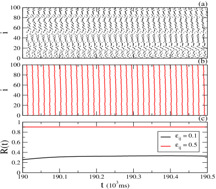
Figure 5: (Colour online) Raster plots of spike onsets for a random network with $100$ Hodgkin-Huxley neurons, $\gamma=0$, (a) $\varepsilon_{\rm ij}=0.1$ and (b) $\varepsilon_{\rm ij}=0.5$. In (c) the time evolution of the Kuramoto order parameter for $\varepsilon_{\rm ij}=0.1$ (black line) and $\varepsilon_{\rm ij}=0.5$ (red line).

3 Spike-Timing Dependent Plasticity

Work carried to try to unveil the role of synaptic plasticity in learning and memory has the Hebb rule as a basis. Hebb rule is a postulate proposed in 1949 by Hebb in his book “The organization of behavior” [30]. He conjectured that the synapse from presynaptic to postsynaptic neuron should be maximally strengthened if the input from presynaptic neuron contributes to the firing of postsynaptic. In this way, a long-term potentiation is caused when there is coincident spiking of presynaptic and postsynaptic neurons [43].

In the synaptic plasticity, synapse weakening and strengthening are implemented by long-term depression (LTD) and potentiation (LTP), respectively [44]. LTP refers to a long-lasting increase in excitatory postsynaptic potential, while LTD decreases the efficacy of a synapse. Bliss et al. [45] suggested that low-frequency firing drives LTD, whereas LTP is driven by presynaptic firing of the high-frequency. Synaptic plasticity alteration as a function of the relative timing of presynaptic and postsynaptic firing was named as spike timing-dependent plasticity (STDP) by Song et al. [46]. STDP has been observed in brain regions, and relevant studies on it were carried out by Gerstner [47] and Markram et al. [48, 49]. Frégnac et al. [50] provided the existence of STDP in cat visual cortex in vivo. Moreover, research on STDP has focused in the hippocampus and cortex [51].

We have studied the changes in synchronous and desynchronous states caused in a Hodgkin-Huxley network due to excitatory (eSTDP), as well as inhibitory (iSTDP) spike timing-dependent plasticity. We have considered the plasticity as a function of the difference of postsynaptic and presynaptic excitatory and inhibitory firing according to Refs. [34] and [35], respectively.

The excitatory eSTDP is given by

$$\Delta\varepsilon_{ij}=\left\{\begin{array}[]{ll}\displaystyle A_{1}\exp(-\Delta t_{ij}/\tau_{1})\;,\;\Delta t_{ij}\geq 0\\ \displaystyle-A_{2}\exp(\Delta t_{ij}/\tau_{2})\;,\;\Delta t_{ij}<0\end{array}\right.,$$ (14)

where

$$\Delta t_{ij}=t_{i}-t_{j}=t_{\rm pos}-t_{\rm pre},$$ (15)

$t_{\rm pos}$ is the spike time of the postsynaptic neuron, and $t_{\rm pre}$ is the spike time of the presynaptic one.

Figure 6(a) shows the result obtained from Eq. (14) for $A_{1}=1.0$, $A_{2}=0.5$, $\tau_{1}=1.8$ms, and $\tau_{2}=6.0$ms. The initial synaptic weights $\varepsilon_{ij}$ are normally distributed with mean and standard deviation equal to $0.25$ and $0.02$, respectively ($0\leq\varepsilon_{ij}\leq 0.5$). They are updated according to Eq. (14), where

$$\varepsilon_{ij}\rightarrow\varepsilon_{ij}+10^{-3}\Delta\varepsilon_{ij}.$$ (16)

The green dashed line denotes the intersection between the absolute values of the depression (black line) and potentiation (red line) curves. For $\Delta t_{c}^{Exc}<1.8$ms the potentiation is larger than the depression. In addition, the red line denotes the absolute value of the coupling strength ($|\Delta\varepsilon_{ij}|$).

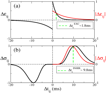
Figure 6: Plasticity as a function of the difference of spike timing of postsynaptic and presynaptic synapses for (a) excitatory (eSTDP) and (b) inhibitory (iSTDP). The green dashed line indicates the intersection between the potential and depression curves.

In the inhibitory iSTDP synapses, the coupling strength $\sigma_{ij}$ is adjusted according to the equation

$$\Delta\sigma_{ij}=\frac{g_{0}}{g_{\rm norm}}{\alpha}^{\beta}|\Delta t_{ij}|{\Delta t_{ij}}^{\beta-1}\exp(-\alpha|\Delta t_{ij}|),$$ (17)

where $g_{0}$ is the scaling factor accounting for the amount of change in inhibitory conductance induced by the synaptic plasticity rule, and $g_{\rm norm}={\beta}^{\beta}\exp(-\beta)$ is the normalising constant. In Figure 6(b) we see the result obtained from Eq. (17) for $g_{0}=0.02$, $\beta=10.0$, $\alpha=0.94$ if $\Delta t_{ij}>0$, and for $\alpha=1.1$ if $\Delta t_{ij}<0$. As a result, $\Delta\sigma_{ij}>0$ for $\Delta t_{ij}>0$, and $\Delta\sigma_{ij}<0$ for $\Delta t_{ij}<0$. The initial inhibitory synaptic weights $\sigma_{ij}$ are normally distributed with mean and standard deviation equal to $\sigma=c\varepsilon$ ($1\leq c\leq 3$) and 0.02, respectively ($0\leq\sigma_{ij}\leq 2c\varepsilon$). The coupling strengths are updated according to Eq. (17), where

$$\sigma_{ij}\rightarrow\sigma_{ij}+10^{-3}\Delta\sigma_{ij}.$$ (18)

The updates for $\varepsilon_{ij}$ and $\sigma_{ij}$ are applied to the last postsynaptic spike. For $\Delta t_{c}^{\rm Inhib}<9.8$ms the depression is larger than the potentiation.

4 Influence of the Synaptic Plasticity on the Network Topology

4.1 Without External Perturbation

About $20\%$ of the synapses in the brain have inhibitory characteristics [52]. We consider that the intensities of both excitatory and inhibitory synapses are modifiable over time by a plasticity rule. We use a network of $200$ Hodgkin-Huxley neurons with $I_{i}$ normally distributed in the interval [$9.0$-$10.0$]. $E_{i}$ represents the $i$-th excitatory neurons with sub-index $i$ in the interval [$1$-$160$] and $I_{i}$ represents the $i$-th inhibitory neuron with the sub-index $i$ in [$161$-$200$]. In all the simulations, we consider a total time interval of $2000$s.

Figure 7: Intensity of the final coupling for initial couplings with $\frac{\sigma}{\varepsilon}=1$ and $\gamma=0$, (a) excitatory and (b) inhibitory synapses. The coupling matrix has a triangular shape.

When the initial intensity of the inhibitory synapses is small ($\frac{\sigma}{\varepsilon}\approx 1$), we show that the potentiation occurs in both kinds of synapses and the final coupling matrix exhibits a triangular shape, as seen in Fig. 7. In the excitatory synapses a reinforcement is observed from the neurons of greater to smaller frequency (Fig. 7(a)), whereas in the inhibitory synapses, the potentiation occurs from the neurons of smaller to greater frequency (Fig. 7(b)). Figure 7(a) points out that presynaptic excitatory neurons that are more likely to strongly connect to a large number of postsynaptic excitatory neurons are also more likely to strongly connect to postsynaptic inhibitory neurons. Similarly, Figure 7(b) points out that presynaptic inhibitory neurons that are more likely to strongly connect to a large number of postsynaptic inhibitory neurons are also more likely to strongly connect to postsynaptic excitatory neurons. This reveal a rich club phenomenon in the neural plasticity, where the neurons with larger degrees to its own ”club” (either the excitatory or the inhibitory community) tend to be also more connected to the other ”club”. The rich-club phenomenon is know to exist in the topological organisation of the brain [53] and was recently hypothetised to be an effect of Hebbian learning mechanisms in Ref. [54].

In Fig. 8 it is exhibited the value of the excitatory $(\bar{\varepsilon})$ and the inhibitory $(\bar{\sigma})$ mean coupling as a function of $\frac{\sigma}{\varepsilon}$. A small variability around the mean values of the excitatory and inhibitory couplings is observed for small values of $\frac{\sigma}{\varepsilon}$. However, increasing the inhibitory synapse implies in an increase in the variability around both mean values, as indicated by the standard deviation bars. This fact becomes notable when the initial intensity of the inhibitory synapses is greater than $\frac{\sigma}{\varepsilon}=1.5$. As a result, the inhibitory synapses act more intensely on the neuronal network dynamics, and a different asymptotic behaviour can be observed. Figures 9 and 10, at $t=2000$s, show the coupling matrices with the values of the excitatory and inhibitory couplings for an initial value given by $\frac{\sigma}{\varepsilon}=2.7$. In some simulations, the synaptic connections tend to zero, namely, the network becomes disconnected (Fig. 9). In other simulations, disconnected blocks are observed, as shown in Fig. 10. Nevertheless, for the same value of the $\frac{\sigma}{\varepsilon}$ parameter, the system can exhibit an asymptotic behaviour similar to the case when initial coupling have $\frac{\sigma}{\varepsilon}=1.0$ (Fig.7).

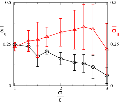
Figure 8: Mean excitatory (black circles) and inhibitory (red triangles) couplings as a function of $\frac{\sigma}{\varepsilon}$, where we consider simulations without external perturbations. The bars indicate the standard deviation calculated for the mean value from 30 simulations.

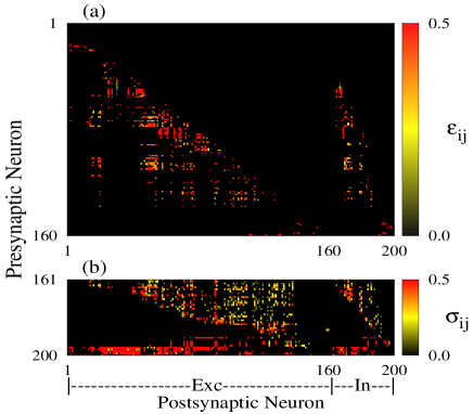
Figure 9: Intensity of the couplings for $\frac{\sigma}{\varepsilon}=2.7$, $\gamma=0$, $t=2000$s, (a) excitatory and (b) inhibitory synapses. The network has disconnected neurons.

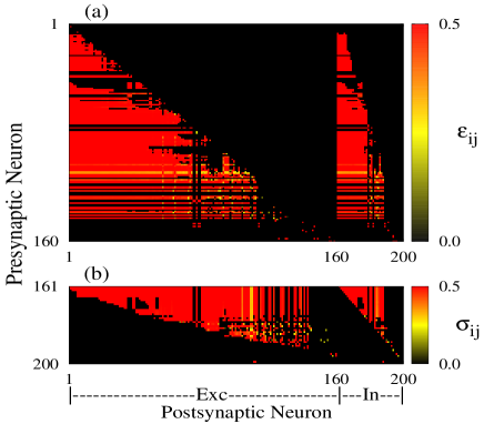
Figure 10: Intensity of the couplings for $\frac{\sigma}{\varepsilon}=2.7$, $\gamma=0$, $t=2000$s, (a) excitatory and (b) inhibitory synapses. The neural network contains disconnected blocks.

The behaviour observed in the synapse intensity can be explained in terms of the average time between spikes. For that, we defined the mean time between spikes among neurons having both excitatory and inhibitory synapses by the equations

$$\bar{\Delta t}_{ij}^{\rm Exc} = \frac{1}{\tau}\sum_{i\neq j}|t_{\rm pre}^{\rm Exc}-t_{\rm pos}|,$$ (19)

$$\bar{\Delta t}_{ij}^{\rm Inhib} = \frac{1}{\tau}\sum_{i\neq j}|t_{\rm pre}^{\rm Inhib}-t_{\rm pos}|.$$ (20)

In Figure 11, $\bar{\Delta t}_{ij}^{\rm Exc}$ and $\bar{\Delta t}_{ij}^{\rm Inhib}$ values are show for the extreme case of initial couplings given by $\frac{\sigma}{\varepsilon}=2.7$ (black lines) and initial coupling given by $\frac{\sigma}{\epsilon}=1.0$ (red lines). For the case where the neuronal network becomes disconnected (black lines), the average time values that are more frequently are found in the depression region of the eSTDP and iSTDP models ($\bar{\Delta t}_{ij}^{\rm Exc}>\Delta t_{c}^{\rm Exc}=1.8\rm ms$ and $\bar{\Delta t}_{ij}^{\rm Inhib}<\Delta t_{c}^{\rm Inhib}=9.8\rm ms$). However, in simulations where a neuronal network becomes strongly connected, a higher concentration of the average time values in the potentiation regions of the plasticity models is observed ($\bar{\Delta t}_{ij}^{\rm Exc}<\Delta t_{c}^{\rm Exc}=1.8\rm ms$ and $\bar{\Delta t}_{ij}^{\rm Inhib}>\Delta t_{c}^{\rm Inhib}=9.8\rm ms$). So, potentiation happening for high frequencies excitatory synapses and lower frequencies inhibitory synapses promote the strengthening of synaptic connectivity and the rich-club phenomenon.

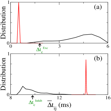
Figure 11: Probability distribution frequency of the average firing times for $\frac{\sigma}{\varepsilon}=2.7$, $\gamma=0$, (a) excitatory and (b) inhibitory synapses. For the triangular shape and unidirectionally connected coupling matrix (Fig. 7), the $\bar{\Delta t_{ij}}$ values are more frequently found in the potentiation regions (red curves in (a) and (b)). The black lines in (a) and (b) illustrate the completely opposite case observed in Fig. 9. The values of $\Delta t_{c}$ were obtained in Fig. 6.

4.2 With External Perturbation

An external perturbation combined with eSTDP and iSTDP can provide a positive contribution to the excitatory and inhibitory mean coupling. In this case, we observe that when the influence of the inhibitory is smaller than the excitatory synapse ($\frac{\sigma}{\varepsilon}<2.3$), the potentiation occurs in approximately all the synapses (excitatory and inhibitory) (Fig. 12). Then, the network remains strongly connected, with a topology close to all-to-all. Almost all the intensities of the connections converge to high values (${\bar{\varepsilon}}_{ij}\geq 0.4$ and ${\bar{\sigma}}_{ij}\approx 0.5$). Only a few connections, where the presynaptic neurons have lower frequency, tend to zero.

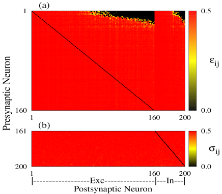
Figure 12: Perturbed intensity of the final coupling for $\frac{\sigma}{\varepsilon}=2.2$, $\gamma=10\mu\rm A/cm^{2}$, (a) excitatory and (b) inhibitory synapses. Almost all connections in the neuronal networks are reinforced.

For larger $\frac{\sigma}{\varepsilon}$ values, we also observe that the inhibitory connections become strengthened. The inhibitory mean coupling converges to the largest value allowed in the interval when $\frac{\sigma}{\varepsilon}>2.3$. However, for this same value of $\frac{\sigma}{\varepsilon}$, there is a trend of decreasing intensity of excitatory synapses ($\bar{\varepsilon_{ij}}\approx 0$). The neurons remain connected through the inhibitory synapses (Fig. 13).

An abrupt transition in the mean excitatory coupling values can also be seen for $\frac{\sigma}{\varepsilon}\approx 2.3$. For values slightly less than $2.3$ ($\frac{\sigma}{\varepsilon}=2.2$), both excitatory and inhibitory synapses undergo an increase in their intensities, whereas, for values of $\frac{\sigma}{\varepsilon}$ larger than this threshold, the inhibitory synapses undergo potentiation while the excitatory synapses tend to zero (Fig. 14).

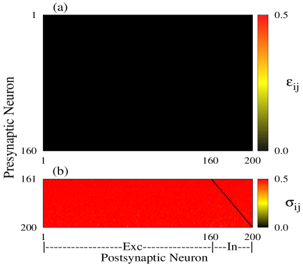
Figure 13: Perturbed intensity of the final coupling for for initial coupling given by $\frac{\sigma}{\varepsilon}=2.4$, $\gamma=10\mu\rm A/cm^{2}$, (a) excitatory and (b) inhibitory synapses. All the excitatory connections in the neuronal networks disappear, but the inhibitory synapses are enhanced.

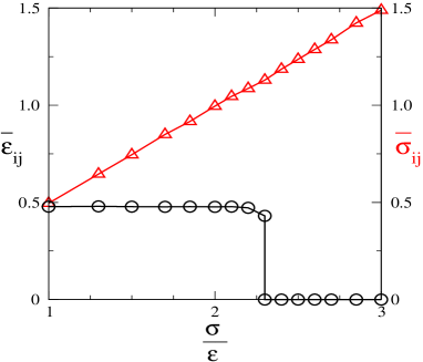
Figure 14: Perturbed mean excitatory (black circles) and inhibitory (red triangles) couplings as a function of $\frac{\sigma}{\varepsilon}$, where we consider $\gamma=10\mu\rm A/cm^{2}$.

The time evolution of both excitatory and inhibitory synapses depend on the time interval between spikes of presynaptic and postsynaptic neurons. Figure 15 shows the frequency between the mean times among presynaptic and postsynaptic spikes. This figure exhibits the two extreme cases, when the neuronal network converges to a strongly connected global topology or to a network with only inhibitory synapses, for $\frac{\sigma}{\varepsilon}=2.3$. When the increase of the weights occurs in almost all the synapses, the $\bar{\Delta t_{ij}}$ values appear more frequently in the regions of potentiation of both models of plasticity ($\bar{\Delta t}_{ij}^{\rm Exc}<\Delta t_{c}^{\rm Exc}=1.8\rm ms$ and $\bar{\Delta t}_{ij}^{\rm Inhib}>\Delta t_{c}^{\rm Inhib}=9.8\rm ms$). However, when only strong inhibitory synapses are observed in the final neuronal network, it is verified that $\bar{\Delta t_{ij}}$ values in excitatory synapses are more frequently found in the depression region of the eSTDP model ($\bar{\Delta t}_{ij}^{\rm Exc}>\Delta t_{c}^{\rm Exc}=1.8\rm ms$). In this case, the inhibitory synapses are reinforced due to the fact that the $\bar{\Delta t_{ij}}$ values are more frequently found in the region of potentiation of the iSTDP model (${\Delta t}_{ij}^{\rm Inhib}>\Delta t_{c}^{\rm Inhib}=9.8\rm ms$).

Therefore, noise can always enhance inhibitory synapses in the plastic brain. Excitatory synapses can also be enhanced if the initial network has sufficiently large excitatory synaptic strength (no less than about half the value of the inhibitory synapses strength).

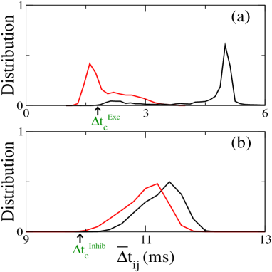
Figure 15: Probability distribution function of the average firing times for $\frac{\sigma}{\varepsilon}=2.3$, $\gamma=10\mu\rm A/cm^{2}$, (a) excitatory and (b) inhibitory synapses. For all-to-all topology (Fig 12, the $\bar{\Delta t_{ij}}$ vales are more frequently found in the potentiation regions (red curves in (a) and (b)). The black lines in (a) and (b) illustrate the completely opposite case observed in Fig. 13. The values of $\Delta t_{c}$ were obtained from Fig. 6.

5 Influence of the Synaptic Plasticity on the Synchronous Behaviour

5.1 Without External Perturbation

The change in the behaviour of the synapse intensity between presynaptic and postsynaptic neurons due to plasticity is reflected on the spike synchronisation. In Fig. 16 we observe different behaviours in relation to synchronisation, where we calculate the order parameter. Figure 16 exhibits the behaviour of the order parameter as a function of time for simulations without external perturbations, discarding a large transient time. The neuronal network evolves to the strong synchronised state with $R(t)>0.9$ (black line) if the initial ratio of intensities of the inhibitory synapses are weak ($\frac{\sigma}{\varepsilon}\approx 1.0$), this inhibition and excitation have similar initial strengths. However, with the increase of the inhibitory synapses intensities $\frac{\sigma}{\varepsilon}>1.5$, different final states are observed in relation to the synchronisation (red, green and blue lines).

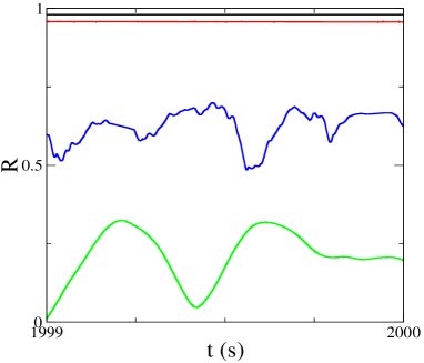
Figure 16: Order parameter for $\frac{\sigma}{\varepsilon}=1.0$ (black line) and $\frac{\sigma}{\varepsilon}=2.7$ (red, blue and green lines).

5.2 With External Perturbation

We consider an external perturbation ($\gamma=10\mu\rm A/cm^{2}$) when the initial inhibitory synapses intensity ratio are small ($\frac{\sigma}{\varepsilon}\approx 1.0$). In this case, the network has a synchronous behaviour ($\bar{R}(t)>0.9$), as shown in Fig. 17 (black line). When inhibitory synapses intensities have a great influence on the network dynamics ($\frac{\sigma}{\varepsilon}\approx 3.0$), neurons tend to exhibit desynchronised firing behaviour with $\bar{R}(t)\approx 0.1$ (red line). However, when $\frac{\sigma}{\varepsilon}\approx 2.3$, we observe two possible asymptotic values for the order parameter. In some simulations a strongly synchronised behaviour appears, while in others it is observed a weakly synchronous evolution of spikes between the neurons in the network (green and blue lines).

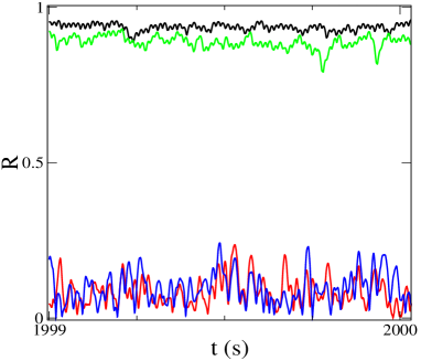
Figure 17: Order parameter for $\gamma=10\mu\rm A/cm^{2}$, $\frac{\sigma}{\varepsilon}=1.0$ (black line), $\frac{\sigma}{\varepsilon}=3.0$ (red line) and $\frac{\sigma}{\varepsilon}=2.3$ (blue and green lines).

6 Conclusions

Neuronal networks based on the Hodgkin-Huxley model have been used to simulate coupled spiking neurons. The Hodgkin-Huxley neuron is a coupled set of ordinary nonlinear differential equations that describes the ionic basis of the membrane potential. In this review, we considered a Hodgkin-Huxley network with synaptic plasticity (STDP). The STDP is a process that adjusts the strength of the synapses in the brain according to time interval between presynaptic and postsynaptic spikes.

We studied the effects of STDP on the topology and spike synchronisation. Regarding the final topology and depending on the balance between inhibitory and excitatory couplings, the network can evolve not only to different coupling strength configurations, but also to different connectivities.

When the strength of the inhibitory connections is of the same order of that of the excitatory connections, the final topology in the plastic brain exhibits the rich-club phenomenon, where neurons that have high degree connectivity towards neurons of the same presynaptical group (either excitatory of inhibitory) become strongly connected to neurons of the other postsynaptical group, i.e., a presynaptical neuron that is highly connected to presynaptical excitatory neurons (or inhibitory ones) becomes strongly connected to postsynaptical inhibitory (or excitatory ones).

When the strength of the synapses becomes reasonably larger than the strength of the excitatory connections, then the final topology has all the features of a complex topology, where neurons only sparsely connect to other neurons with a non-trivial topology.

When noise is introduced in the neural network, we observe that inhibitory synapses are always enhanced in the plastic brain. Excitatory synapses can also be enhanced if the initial network has sufficiently large excitatory synaptic strength (no less than about half the value of the inhibitory synapsis strength).

The changes in the synapse strength and the connectivities due to STDP produce significant alterations in the synchronous states of the neuronal network. We observe that the synchronous states depend on the balance between the excitatory and inhibitory intensities. We also find coexistence of strongly synchronous and weakly synchronous behaviours.

References

- [1] W. Gerstner, W. Kistler, Spiking neuron models: Single neurons, populations, plasticity (Cambridge University Press, Cambridge, 2002)
- [2] O. Sporns, G. Tononi, R. Kötter. PLoS Comput. Biol. 1(4), e42 (2005)
- [3] R.L. Viana, F.S. Borges, K.C. Iarosz, A.M. Batista, S.R. Lopes, I.L. Caldas. Commun. Nonlinear Sci. Numer. Simul. 19(1), 164 (2014)
- [4] F.S. Borges, E.L. Lameu, A.M. Batista, K.C. Iarosz, M.S. Baptista, R.L. Viana. Physica A 430, 236 (2015).
- [5] S. Wolfram. Rev. Mod. Phys. 55(3), 601 (1983)
- [6] C.A.S. Batista, E.L. Lameu, A.M. Batista, S.R. Lopes, T. Pereira, G. Zamora-López, J. Kurths, R.L. Viana. Phys. Rev. E 86, 016211 (2012)
- [7] E.L. Lameu, F.S. Borges, R.R. Borges, K.C. Iarosz, I.L. Caldas, A.M. Batista, R.L. Viana, J. Kurths. Chaos 26, 043107 (2016)
- [8] E.L. Lameu, F.S. Borges, R.R. Borges, A.M. Batista, M.S. Baptista, R.L. Viana. Commun. Nonlinear Sci. Numer. Simul. 34, 45 (2016)
- [9] M. Girardi-Schappo, G.S. Bortolotto, R.V. Stenzinger, J.J. Gonsalves, M.H.R. Tragtenberg. PLoS ONE 12(3), e0174621 (2017)
- [10] L.F. Abbott. Brain Res. Bull. 50, 303 (1999)
- [11] C.A.S. Batista, R.L. Viana, S.R. Lopes, A.M. Batista. Physica A 410, 628 (2014)
- [12] M.S. Baptista, F.M. Kakmeni, C. Grebogi. Phys. Rev. E 82, 036203 (2010)
- [13] L. Lapicque. J. Physiol. Pathol. Gen. 9, 620 (1907)
- [14] A.L. Hodgkin, A.F. Huxley. J. Physiol. 117, 500 (1952)
- [15] L.J. Hindmarsh, R.M. Rose. Proc. R. Soc. Lond. B 221, 87 (1984)
- [16] M.S. Baptista, J. Kurths. Phys. Rev. E 77, 026205 (2008)
- [17] M.S. Baptista, J.X. de Carvalho, M.S. Hussein. PloS ONE 3, e3479 (2008)
- [18] C.G. Antonopoulos, S. Srivastava, S.S. Pinto, M.S. Baptista. PLoS Comput. Biol. 11, e1004372 (2015)
- [19] P. Uhlhaas, G. Pipa, B. Lima, L. Melloni, S. Neuenschwander, D. Nikolić, W. Singer. Front. Integr. Neurosci. 3, 17 (2009)
- [20] L. Melloni, C. Molina, M. Pena, D. Torres, W. Singer, E. Rodriguez. J. Neurosci. 27(11), 2858 (2007)
- [21] F.S. Borges, P.R. Protachevicz, E.L. Lameu, R.C. Bonetti, K.C. Iarosz, I.L. Caldas, M.S. Baptista, A.M. Batista. Neural Netw. 90, 1 (2017)
- [22] J. Fell, N. Axmacher. Nat Rev. Neurosci. 12, 105 (2011)
- [23] L.L. Rubchinsky, C. Park, R.M. Worth. Nonlinear Dyn. 68, 329 (2012)
- [24] E.L. Lameu, F.S. Borges, R.R. Borges, K.C. Iarosz, I.L. Caldas, A.M. Batista, R.L. Viana, J. Kurths. Chaos 26, 043107 (2016)
- [25] E.L. Bennett, M.C. Diamond, D. Krech, M.R. Rosenzweig. Science 146, 610 (1964)
- [26] W. James, The principles of psychology (Henry Holt and Company, New York, 1890)
- [27] K.S. Lashley. Psychol. Bull. 30, 237 (1923)
- [28] E.L. Bennett, M.C. Diamond, D. Krech, M.R. Rosenzweig. Science 146, 610 (1964)
- [29] M.C. Diamond, D. Krech, M.R. Rosenzweig. J. Comp. Neurol. 123, 111 (1964)
- [30] D.O. Hebb, The organization of behavior (Wiley, New York, 1949)
- [31] W. Gerstner, H. Sprekeler, G. Deco. Science 338, 60 (2012)
- [32] H. Markram, W. Gerstner, P.J. Sjostrom. Front. Synaptic Neurosci. 4, 1 (2012)
- [33] R.R. Borges, F.S. Borges, E.L. Lameu, A.M. Batista, K.C. Iarosz, I.L. Caldas, R.L. Viana, M.A.F. Sanjuán. Commun. Nonlinear Sci. Numer. Simul. 34, 12 (2016)
- [34] G.-Q. Bi, M.-M. Poo. J. Neurosci. 18(24), 10464 (1998)
- [35] J.S. Haas, T. Nowotny, H.D.I. Abarbanel. J. Neurophysiol. 96, 3305 (2006)
- [36] B. Alberts, A. Johnson, J. Lewis, M. Raff, K. Roberts, P. Walter, Molecular biology of the cell, 4th ed. (Garland Science, New York, 2002)
- [37] M.A. Arbib, The handbook of brain theory and neural networks (The MIT Press, Cambridge 2002)
- [38] E. Gouaux, R. Mackinnon. Science 310(5), 344 (2009)
- [39] A. Arenas, A. Díaz-Guilera, J. Kurths, Y. Moreno, C. Zhou. Phys. Rep. 469, 93 (2008)
- [40] G. Deco, A. Buehlmann, T. Masquelier, E. Hugues. Front. Hum. Neurosci. 5, 1 (2011)
- [41] V.O. Popovych, S. Yanchuk, P.A. Tass. Sci. Rep. 3, 2926 (2013)
- [42] Y. Kuramoto, Chemical oscillations, waves, and turbulence (Springer, Berlin, 1984)
- [43] W. Gerstner. Front. Synaptic Neurosci. 2, 1 (2010)
- [44] D.E. Feldman. Neuron 75, 556 (2012)
- [45] T.V. Bliss, T. Lomo. J. Physiol. 232, 331 (1973)
- [46] S. Song, K.D. Miller, L.F. Abbott. Nat. Neurosci. 3, 919 (2000)
- [47] W. Gerstner, R. Kempter, J.L. van Hemmen. Nature 383, 76 (1996)
- [48] H. Markram, B. Sakmann. Soc. Neurosci. Abstr. 21, 1 (2007)
- [49] H. Markram, J. Lübke, M. Frotscher, B. Sakmann. Science 275, 213 (1997)
- [50] Y. Frégnac, M. Pananceau, A. René, N. Huguet, O. Marre, M. Levy, D.E. Schulz. Front. Synaptic Neurosci. 2, 73 (2010)
- [51] K.A. Buchanan, J. R. Mellor. Front. Synaptic Neurosci. 2, 94 (2010)
- [52] C.R. Noback, N.L. Strominger, R.J. Demarest, D.A. Ruggiero, The human nervous systems: Structure and function, 6th ed. (NJ: Humana Press, Totowa, 2005)
- [53] E.K. Towlson, E. Vértes, S.E. Anhert, W.R. Schafer, E.T. Bullmore. J. Neurosc. 33, 6380 (2013)
- [54] P.E. Vértes, A. Alexander-Bloch, E.T. Bullmore. Philos. Trans. R. Soc. Lond. B Biol. Sci. 369, 20130531 (2014)