Stability and boundedness in AdS/CFT
with double trace deformations

Steven Casper¹, William Cottrell^1,2, Akikazu Hashimoto¹,

Andrew Loveridge¹, and Duncan Pettengill¹

¹ Department of Physics, University of Wisconsin, Madison, WI 53706, USA

² Institute for Theoretical Physics Amsterdam, University of Amsterdam

1098 XH Amsterdam, The Netherlands

Scalar fields on the bulk side of AdS/CFT correspondence can be assigned unconventional boundary conditions, related to the conventional one by Legendre transform. One can further perform double trace deformations which relate the two boundary conditions via renormalization group flow. Thinking of these operators as $S$ and $T$ transformations, respectively, we explore the $SL(2,{\bf R})$ family of models which naively emerges from repeatedly applying these operations. Depending on the parameters, the effective masses vary and can render the theory unstable. However, unlike in the $SL(2,{\bf Z})$ structure previously seen in the context of vector fields in $AdS_{4}$, some of the features arising from this exercise, such as the vacuum susceptibility, turns out to be scheme dependent. We explain how scheme independent physical content can be extracted in spite of some degree of scheme dependence in certain quantities.

1 Introduction

In AdS/CFT correspondence, there is a well known dichotomy of alternate boundary conditions originally pointed out by Klebanov and Witten in [1]. The main idea is that the formula for the scaling dimension of scalar operators dual to a bulk scalar of mass $m$ in AdS/CFT correspondence

$$\Delta_{+}={d+\sqrt{d^{2}+4m^{2}}\over 2}$$ (1.1)

also makes sense when one assigns the other branch of the square root

$$\Delta_{-}={d-\sqrt{d^{2}+4m^{2}}\over 2}\ .$$ (1.2)

On the CFT side, the different assignment of dimensions corresponds to defining a different CFT with different operator content. On the bulk side, this dichotomy was interpreted as choice of boundary condition. In the convention where the AdS metric takes the form

$$ds^{2}={r^{2}\over R^{2}}(dt^{2}+d\vec{x}^{2})+{R^{2}\over r^{2}}dr^{2}$$ (1.3)

the scalar fields behave asymptotically as

$$\phi(r)=P_{1}(\vec{x})r^{-\Delta_{-}}(1+\ldots)-P_{2}(\vec{x})(r^{-\Delta_{+}}+\ldots)\ .$$ (1.4)

The standard convention is to fix the coefficient of the dominant term, $P_{1}(\vec{x})$, at the boundary and to infer the expectation value of the dual operator from the value of $P_{2}(\vec{x})$. This is the branch where the dimension of operator is $\Delta_{+}$, and is commonly referred to as the Dirichlet boundary condition for the scalars in anti de Sitter space. In this scheme, $P_{1}(\vec{x})$ interpreted as introducing a source term

$$\exp\left[\int d^{d}x\ P_{1}(\vec{x}){\cal O}(\vec{x})\right]$$ (1.5)

to the CFT path integral.

In the alternate scheme, one fixes the subdomiant coefficient $P_{2}(\vec{x})$ and read off the expectation value of the operator of dimension $\Delta_{-}$ from $P_{1}(\vec{x})$. The role of $P_{1}$ and $P_{2}$ is therefore reversed, and this scheme is referred to as the Neumann scheme.

These two distinct theories were further shown to be related by Legendre transform of the sources [1]. This can be understood as arising naturally on the bulk side as Legendre transform which interchanges the boundary conditions. Klebanov and Witten showed that this leads to expected mapping of the dimensions of operators [1].

The two theories are also related by renormalization group flow induced by double trace deformation [1, 2]. This flow can be visualized as having the Neumann theory as the ultraviolet fixed point, deformed by a double trace operator

$$\int d^{d}x\ \alpha{\cal O}(\vec{x})^{2}$$ (1.6)

whose dimension is

$$[{\cal O}(\vec{x})^{2}]=2\Delta_{-}$$ (1.7)

and so is relevant for

$$2\Delta_{-}<d$$ (1.8)

which is equivalent to the Breitenlohner-Freedman bound, which, combined with the the unitarity bound, leads to constraint

$$-{d^{2}\over 4}<m^{2}<-{d^{2}\over 4}+1.$$ (1.9)

In the infra-red, the flow approaches the Dirichlet fixed point. The double trace deformation is treatable using Hubbard-Stratonovich techniques. The central charges at both the ultraviolet and the infrared fixed points can be computed and was found to decrease along the flow, as expected, at order $N^{0}$ [3, 4]. One can also compute correlation functions and infer the cross-over between $\Delta_{-}$ scaling in the ultraviolet and the $\Delta_{+}$ scaling in the infrared [3, 4]. The double trace deformation therefore introduces a continuous parameter which interpolates between the Dirichlet and the Neumann theories.

So we have introduced two operations, the Legendre transform and the double trace deformation, which acts on the space of theories. This naturally leads one to wonder how these operations act in combination. If one acts with Legendre transform, followed by a double trace deformation, and then again with Legendre transform, is the resulting theory equivalent, or distinct, from purely performing a double trace deformation? In other words, does the double trace deformation and Legendre transform commute? Related to these issues is the question of how one parameterizes the space of theories on which these transformations act.

Closely related issue was considered in the context of bulk vector fields which are dual to current like operator by Witten in [5]. In the setup of Witten, the dimension of bulk was four, and the double trace deformation was related to Chern-Simons term and as a result had quantized coefficients. The act of increasing the Chern-Simons level acted as a discrete $T$-transformation while the Legendre transform acted as $S$-transform, giving rise to an $SL(2,{\bf Z})$ group of transformations. The set of theories then corresponded to the set of $SL(2,{\bf Z})$ elements itself, on which the group of transformations acted by left multiplication.

In this article, we will consider the scalar version of the double trace deformation where the analogue of $S$ and $T$ transformation exists, but where the $T$ transformation is continuous leading to the $SL(2,{\bf R})$ family of theories. On first pass, we will find that the $S$ conjugate of $T$ transformation turns out to be a contact-term which parameterizes scheme dependence. This raises some puzzle regarding the physicality/scheme independence of correlation functions and equations of state. We will explain that scalar correlation functions are indeed scheme dependent, but in such a way that some observables, such as the onset of phase transitions, latent heat, and critical scaling dimensions near a second order phase transitions are scheme independent.

2 $SL(2,R)$ transform of boundary condition and correlation functions

Let us go back to the discussion of scalars, and consider a setup where the bulk geometry is an Eucledian $AdS_{d+1}$-Schwarzschild geometry

$$ds^{2}={r^{2}\over R^{2}}\left(f(r)dt^{2}+d\vec{x}^{2}\right)+{R^{2}\over f(r)r^{2}}dr^{2}$$ (2.1)

with

$$f=1-{r_{0}^{d}\over r^{d}}\ .$$ (2.2)

Regularity requires the $t$ coordinate to be periodic

$$t=t+{1\over T},\qquad T={d\over 4\pi R^{2}}r_{0}\ .$$ (2.3)

We will take $\vec{x}$ to be the coordinates in $(d-1)$ dimensions which we also take to be living on ${\bf T}^{d-1}$ of volume $V_{d-1}$ but whose radii is much larger than $T^{-1}$.

The reason for introducing thermal periodic boundary condition is to regulate some observables in the infrared. It also allows various observables to be interpreted in the context of thermal field theory. Of course, one can just as easily take the zero temperature limit in the end and see how the observables behave if desired.

We consider minimally coupled scalar in this background whose action is

$$S=\int d^{d}x\int dr\,\sqrt{g}\left({1\over 2}g^{rr}(\partial_{r}\Phi)^{2}+{1\over 2}g^{xx}(\partial_{x}\Phi)^{2}+{1\over 2}{m^{2}\over R^{2}}\Phi^{2}\right)$$ (2.4)

where

$$\det g=\left({r^{2}\over R^{2}}\right)^{d-1}\ .$$ (2.5)

and $m$ is dimensionless to match the convention used in (1.1).

We will now concentrate, for time being, on the zero momentum component of the scalar field in the $\vec{x}$ directions, although we will bring the momentum dependence later. Zero momentum component is sufficient for discussing observables such as vacuum susceptibility. It is also convenient to scale out dimensionful quantities by setting

$$r=r_{0}u$$ (2.6)

and

$$\Phi(r)=\left({r_{0}\over R^{2}}\right)^{-(d-1)/2}\phi(u)\ .$$ (2.7)

Then, the action becomes

$$S={\cal N}\int du\ u^{d-1}\left({1\over 2}fu^{2}(\partial_{u}\phi(u))^{2}+{1\over 2}m^{2}\phi(u)^{2}\right)$$ (2.8)

with

$$f=1-u^{-d}$$ (2.9)

and

$${\cal N}={r_{0}V_{d-1}\over R^{d+1}T}\ .$$ (2.10)

In terms of this parametrization, we formulate the generating function $Z[J]$ for scalar operators sourced by $J$ as follows.

$$Z[J] = \int D\phi\exp\left[-{\cal N}\int_{1}^{u_{c}}du\ u^{d-1}\left({1\over 2}fu^{2}(\partial_{u}\phi(u))^{2}+{1\over 2}m^{2}\phi(u)^{2}\right)\right.$$

$$\qquad-{{\cal N}\over 2}\Delta_{-}u_{c}^{d}\phi(u)^{2}$$

$$\qquad\left.\left.\rule{0.0pt}{12.91663pt}+{\cal N}(\Delta_{+}-\Delta_{-})\left(\alpha u_{c}^{2\Delta_{-}}\phi(u_{c})^{2}+u_{c}^{\Delta_{-}}\beta\phi(u_{c})J\right)\right|_{u_{c}\rightarrow\infty}\right]\ .$$

The first line of (2) is the action integrated up to the ultraviolet cut-off at $u=u_{c}$ where $u_{c}$ is eventually taken to infinity. The second line is the standard holographic renormalization counter-term [6]. The third term includes terms proportional to dimensionless parameters $\alpha$ and $\beta$, as well as some dimensionless factor ${\cal N}(\Delta_{+}-\Delta_{-})$ which is included for convenience. They can be absorbed into $\alpha$ and $\beta$ but we find it convenient to separate these factors as we did in (2) for notional purposes. The term proportional to $\alpha$ is recognizable as the double trace term, e.g. the term proportional to $\lambda$ in equation (3.1) of [7].

The third line is also a boundary term specifying the boundary condition. In terms of asymptotic expansion

$$\phi(u)=p_{1}u^{-\Delta_{-}}\left(1+{\cal O}(u^{-1})\right)-p_{2}u^{-\Delta_{+}}\left(1+{\cal O}(u^{-1})\right)$$ (2.13)

the Euler-Lagrange variation at $u=u_{c}$ in the large $u_{c}$ limit imposes the condition

$$J=-{2\alpha\over\beta}p_{1}+{1\over\beta}p_{2}\ .$$ (2.14)

So, if $\alpha=0$, the boundary condition is Neumann. Turning on $\alpha$ corresponds then to the double trace deformation as was the case in the treatment of [3, 4]. The operator sourced by $J$ can also be identified as

$${\cal O}\equiv{1\over(\Delta_{+}-\Delta_{-}){\cal N}}{\delta\over\delta J}=\beta p_{1}\ .$$ (2.15)

This is precisely the prescription for reading off the expectation value in Neumann theories. The natural value to assign to $\beta$ is $\beta=1$. Changing $\beta$ merely affects various normalization conventions.

The issue we wish to explore is how this generating function further transforms under Legendre transform and double trace deformation. We will approach this question by making an educated guess for the answer, and then subjecting the guess to tests.

The ansatz we wish to offer is to write the generating function in the following form

$$Z[J] = \int D\phi\exp\left[-{\cal N}\int_{1}^{u_{c}}du\ u^{d-1}\left({1\over 2}fu^{2}(\partial_{u}\phi(u))^{2}+{1\over 2}m^{2}\phi(u)^{2}\right)\right.$$

$$\qquad-{{\cal N}\over 2}\Delta_{-}u_{c}^{d}\phi(u)^{2}$$

$$\qquad\left.\left.\rule{0.0pt}{12.91663pt}+{\cal N}(\Delta_{+}-\Delta_{-})\left(\alpha u_{c}^{2\Delta_{-}}\phi(u_{c})^{2}+u_{c}^{\Delta_{-}}\beta\phi(u_{c})J+\gamma J^{2}\right)\right|_{u_{c}\rightarrow\infty}\right]\ .$$

The term proportional to $\gamma$ is the new term, and is introduced to close the $SL(2,{\bf R})$ operation. It is the unique term which is missing in the bi-linears of $J$ and $\phi(u_{c})$. One can immediately infer with this ansatz that the expectation value and the boundary condition takes the form

$${\cal O}\equiv{1\over(\Delta_{+}-\Delta_{-}){\cal N}}{\delta\over\delta J} = \left(\beta-{4\alpha\gamma\over\beta}\right)p_{1}+{2\gamma\over\beta}p_{2}$$ (2.18)

$$J = -{2\alpha\over\beta}p_{1}+{1\over\beta}p_{2}\ .$$ (2.19)

which leads one to naturally parameterize $(\alpha,\beta,\gamma)$ in terms of $SL(2,{\bf R})$ matrix

$$\left(\begin{array}[]{cc}a&b\\ c&d\end{array}\right)=\left(\begin{array}[]{cc}\beta-{4\alpha\gamma\over\beta}&{2\gamma\over\beta}\\ -{2\alpha\over\beta}&{1\over\beta}\end{array}\right)$$ (2.20)

and in this parametrization, setting $\gamma=1$ and $\beta=1$ gives rise naturally to

$$\left(\begin{array}[]{cc}a&b\\ c&d\end{array}\right)=\left(\begin{array}[]{cc}1&0\\ -2\alpha&1\end{array}\right)$$ (2.21)

which is clearly the $T$ element of $SL(2,{\bf R})$. One can also verify that starting with some generic values of $(\alpha,\beta,\gamma)$ and performing Legendre transform gives rise to new set of $(\alpha,\beta,\gamma)$ which corresponds to acting on $SL(2,{\bf R})$ parametrization by left multiplication by the $S$ element. As such, we can conclude that (2) is the general expression on which the Legendre transform and double trace deformation can act.

Although we presented the analysis focusing on the zero momentum modes along the boundary, it is straight forward to generalize the analysis to non-zero modes, by writing

$$Z[J] = \int D\phi\exp\left[-{\cal N}\sum_{\vec{k}}\int_{1}^{u_{c}}du\ u^{d-1}\left({1\over 2}fu^{2}\partial_{u}\phi_{\vec{k}}(u)\partial_{u}\phi_{-\vec{k}}(u)+{1\over 2}m^{2}\phi_{\vec{k}}(u)\phi_{-\vec{k}}(u)\right)\right.$$

$$\qquad-{{\cal N}\over 2}\Delta_{-}u_{c}^{d}\phi_{\vec{k}}(u)\phi_{-\vec{k}}(u)$$

$$\qquad\left.\left.\rule{0.0pt}{12.91663pt}+{\cal N}(\Delta_{+}-\Delta_{-})\left(\alpha u_{c}^{2\Delta_{-}}\phi_{\vec{k}}(u_{c})\phi_{-\vec{k}}(u_{c})+u_{c}^{\Delta_{-}}\beta\phi_{\vec{k}}(u_{c})J_{-\vec{k}}+\gamma J_{\vec{k}}J_{-\vec{k}}\right)\right|_{u_{c}\rightarrow\infty}\right]$$

where the $d$ dimensional momentum label $\vec{k}$ is discrete since we have compactified all spatial dimensions.

In this form, it is straightforward to compute the normalized two point function

$$G(\vec{k})\equiv{1\over(\Delta_{+}-\Delta_{-}){\cal N}}{\delta\over\delta J_{\vec{k}}}{\delta\over\delta J_{-\vec{k}}}Z[J]={aG_{N}(\vec{k})+b\over cG_{N}(\vec{k})+d}$$ (2.24)

where

$$G_{N}(\vec{k})={dp_{1}(\vec{k})\over dp_{2}(\vec{k})}$$ (2.25)

is the two point function for the Neumann boundary condition. For the case of $d=2$ in the large volume limit for $\vec{k}$ entirely in the spatial direction, this can be computed in closed form and takes the form

$$G_{N}(k)=\frac{\Gamma(1+\nu)\Gamma\left(\frac{1}{2}(1-\nu-ik)\right)\Gamma\left(\frac{1}{2}(1-\nu+ik)\right)}{\Gamma(1-\nu)\Gamma\left(\frac{1}{2}(1+\nu-ik)\right)\Gamma\left(\frac{1}{2}(1+\nu+ik)\right)},\qquad\nu=\sqrt{1+m^{2}}\ .$$ (2.26)

The values of $(a,b,c,d)$ are determined in terms of $(\alpha,\beta,\gamma)$ by (2.20). The expression (2.24) shows that the two point function for generic $(\alpha,\beta,\gamma)$ is parameterized naturally in terms of $SL(2,{\bf R})$. We have also seen how the boundary condition (2.19) and the operator (2.18) is parameterized in terms of the $SL(2,{\bf R})$ data. So in a certain sense, it is natural to think of the space of theories as also being parameterized in terms of $SL(2,{\bf R})$. This is the main result of this article. The implication and the interpretation of this result is discussed in the following section.

The group $SL(2,{\bf R})$ has three generators. Aside from the double trace and contact term deformations, there is a relatively trivial deformation (when $\alpha=\gamma=0$)

$$\left(\begin{array}[]{cc}a&b\\ c&d\end{array}\right)=\left(\begin{array}[]{cc}\beta&0\cr 0&\beta^{-1}\end{array}\right)\ .$$ (2.27)

Left multiplication by this element essentially amounts to adjusting the normalization of ${\cal O}$ and as such is physically trivial. Although the group manifold of $SL(2,{\bf R})$ is $AdS_{3}$ and is three dimensional, one might be tempted to collapse the parameter space from three to two by quotienting the space of theories with respect to left multiplication by this hyperbolic element of $SL(2,{\bf R})$. Unfortunately, this introduces a multi-component quotient space exactly analogous to what one finds when constructing the BTZ orbifold by modding out with a discrete choice of $\beta$’s [8]. We find it more convenient to include this trivial scaling as part of the theory space whose geometry is familiar.

3 Discussions

In the previous section, we presented a parametrization of generating functional (2) and (2) with parameters $(\alpha,\beta,\gamma)$ related to $SL(2,{\bf R})$ parameters by (2.20) such that

• Setting the parameters

  $$\left(\begin{array}[]{cc}a&b\\ c&d\end{array}\right)=\left(\begin{array}[]{cc}1&0\\ 0&1\end{array}\right)$$ (3.1)

  corresponds to the Neumann theory.

• Acting with $T$ deformation

  $$\left(\begin{array}[]{cc}a&b\\ c&d\end{array}\right)=\left(\begin{array}[]{cc}1&0\\ -2\alpha&1\end{array}\right)$$ (3.2)

  corresponds to turning on the double trace deformation

• Acting with $S$ deformation.

  $$\left(\begin{array}[]{cc}a&b\\ c&d\end{array}\right)=\left(\begin{array}[]{cc}0&-1\\ 1&0\end{array}\right)$$ (3.3)

  corresponds to Legendre transform.

One can therefore interpret the generic model parameterized by $SL(2,{\bf R})$ as arising from successive action of $T$ and $S$ transformations. These data manifest themselves in observables through relations (2.18) and (2.19). We will now comment on the interpretation of these results.

First observation we wish to make is the fact that the dependence on $\gamma$ in (2) and (2) is merely that of a contact term. In other words, they do not contribute to the correlation function in position space at finite separation. This can also be seen by re-writing the two point function (2.24) in the form

$$G(\vec{k}) = {1\over c(cG_{N}(k)+d)}+{a\over c}\qquad(c\neq 0)$$ (3.4)

$$G(\vec{k}) = {1\over d^{2}}G_{N}(k)+{b\over d}\qquad\qquad\ (c=0)\ .$$ (3.5)

From this expression and (2.20), we see that the pole structure only depends on $\alpha$. The dependence on $\gamma$ is only in the constant additive term $a/c$. This is also reflected in the fact that the boundary condition (2.19) does not depend $\gamma$ and as a result, the spectrum of small fluctuations are insensitive to this $\gamma$. So, although we have identified an $SL(2,{\bf R})$ family of partition function (2) and (2), we conclude that its physical manifestation is mostly trivial.

There is however one subtlety in the interpretation of the dependence on $\gamma$. The vacuum susceptibility

$$\chi\equiv G(k=0)={\cal N}(\Delta_{+}-\Delta_{-})\langle{\cal O}_{\vec{k}=0}{\cal O}_{\vec{k}=0}\rangle$$ (3.6)

which parameterizes the stability of the vacuum is expected positive definite by fluctuation dissipation theorem and is manifest in the form of the right hand side of (3.6). Indeed, for the Neumann theory, one finds $\chi$ to be a positive number of order one. However, for general $(\alpha,\beta,\gamma)$, $\chi$ will inherit the non-trivial dependence on $\gamma$ through (2.24). For the Dirichlet model one obtains by taking the Legendre transform of the Neumann theory, this susceptibility will turn out to be negative despite the fact that the theory is expected to be sensible. By contrast, small deformation of Neumann theory by double trace deformation (2), which is expected to flow to the Dirichlet theory in the infrared, has a positive susceptibility. How does one make sense of all of these facts?

The answer is simply that the vacuum susceptibility is dependent on contact terms because contact terms contribute at all momenta including the zero mode. The contact term itself should be considered as the artifact of renormalization scheme dependence. The situation here is different from that which was considered in [5] where the large gauge transformations constrained the analogue of our counter-terms to take on discrete scheme independent values.

It seems that for the scalars, vacuum susceptibility is a scheme dependent observable and must be calibrated by some renormalization condition. This then suggests that susceptibility can not be treated as an unambiguous (scheme independent) physical feature. If one accepts this, however, the meaning of holographic second order phase transitions such as [9, 10, 11], whose salient feature is the vanishing of vacuum susceptibility, all of a sudden becomes mysterious. How can one probe the behavior of vacuum susceptibility switching signs when vacuum susceptibility itself is scheme dependent?

To answer this question, we need to recall the fact that the momentum expansion of the effective action for the order parameter [12]

$$v_{\vec{k}}=\langle{\cal O}_{\vec{k}}\rangle$$ (3.7)

is given by the inverse of the two point function

$$G(k)^{-1}=c_{0}+c_{2}k^{2}+c_{4}k^{4}+\ldots\ .$$ (3.8)

For the setup based on thermal AdS/CFT under consideration, one expects all of these coefficients to generically be of order one, which in our parametrization scheme (2.6) corresponds to the scale being set by the temperature. (We are assuming that the radius of the spatial coordinates is much larger than the radius of the thermal circle.) However, if for some special choice of parameters $(\alpha,\beta,\gamma)$ one finds

$$c_{0}\ll c_{2}\sim c_{4}\sim\ldots$$ (3.9)

then one finds a light effective degree of freedom whose mass is of order

$$m^{2}={c_{0}\over c_{2}}$$ (3.10)

in units set by the temperature. So only when $c_{0}$ happens to be small, one expects an effective field theory description to be useful, but this is precisely the regime near the second order phase transition.

It is interesting to examine the behavior of the susceptibility and the effective mass of our simple system (2) starting with the Neumann system with $\beta=1$, and gradually increasing $\alpha$, keeping $\gamma$ at fixed zero. For the Neumann theory, one has positive susceptibility and a positive effective mass squared of order one in thermal units. As $\alpha$ is increased, however, the effective mass decreases, until one reaches the point where

$$\alpha={1\over 2G_{N}(k=0)}\ .$$ (3.11)

At this point, the system develops a tachyon and the susceptibility flips sign. This is the tachyonic behavior previously discussed by Troost in [13]. If this system is stabilized by coupling to some other non-linear system, one expects to find a second order phase transition around this point.

Furthermore, one sees in (3.8) that this is precisely when susceptibility is going to infinity. But then since the susceptibility is infinite, additive contribution from $\gamma$ is essentially irrelevant. In other words, even though the specific values of the susceptibility at generic point in the $SL(2,{\bf R})$ parameter space is scheme dependent, the locus, and the behavior near, the critical point is scheme independent.

To the extent that the contact term is affecting the operator (2.18), one can think of the scheme dependence though contact terms as field reparameterization ambiguity of the order parameter. The reason that the effective field theory treatment works well despite such ambiguity is the fact that the behavior near the critical point is insensitive to such reparameterization ambiguities, and the same principle is at work in the holographic setup.

In essence, we are merely making a simple observation that effective field theory analysis is reliable specifically when describing the dynamics of some degree of freedom whose effective mass is much lighter than the characteristic mass scale of the rest of the system. In the context of $SL(2,{\bf R})$ family, we can reliably assess when the condition for when such an effective description is valid, and infer scheme independent universal features.

An interesting issue to further explore is the extent to which global stability issues such as Gibbs ruling of convex free energies (see e.g. [14]) is realized in light of some of these scheme dependencies. Naively, there appears to be some tension between scheme independence only for the near critical behavior of these systems, which is local, in contrast to the constraints based on global stability issues. Understanding this issue in a certain intersecting brane system [15] was our original motivation to explore these issues. One can in fact see that coexistence of states and the condition for first order phase transition to take place is unaffected by the contact term deformations, as one would expect on physical grounds, by the following argument. Thinking of $p_{2}(p_{1})$ as the equation of state with $p_{1}$ playing the role of order parameter, the condition for two states to coexist at some fixed external $\bar{p}_{2}$ is for there to be multiple $p_{1}$ satisfying the condition

$$p_{2}(p_{1}^{a})=p_{2}(p_{1}^{b})=\bar{p}_{2}\ .$$ (3.12)

The difference in free energy for the stationary states at $p_{1}=p_{1}^{a}$ and $p_{1}=p_{1}^{b}$ is then

$$\Delta F=\int_{p_{1}^{a}}^{p_{1}^{b}}dp_{1}\,(p_{2}-\bar{p}_{2})\ .$$ (3.13)

Now, the reparameterization of order parameter (2.18) transforms $p_{1}$ into $p_{1}+\gamma p_{2}$. But then

$$\Delta F^{\prime}=\int_{p_{1}^{a}}^{p_{1}^{b}}(dp_{1}+\gamma dp_{2})(p_{2}-\bar{p}_{2})=\Delta F\ .$$ (3.14)

The term proportional to $\gamma$ then drops out because the integral starts and ends at the same value of $p_{2}$. So the $\Delta F$ after the contact term deformation is unchanged. The equilibrium configuration is the one with the lowest free energy. If there are multiple degenerate global minimum, then the system can exist in coexistence giving rise to a Gibbsian ruling. So the precise form of the free energy as a function of the order parameter remains scheme dependent, but the possible existence of coexistence states and the subsequent Gibbsian ruling is unaffected. This point can be illustrated, as we have done in figure 1, by drawing how the free energy transforms under field redefinition of the order parameter. It would be interesting to further explore the consequences of this observation in varoius holographic thermodynamic systems including [15].

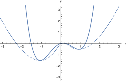
Figure 1: In this figure, we illustrate how a hypothetical free energy $F(v)$ (undotted) is transformed under field redefinition (2.18) of the order parameter $v^{\prime}=v+\gamma{dF\over dv}$ (dotted) for some parameter $\gamma$. The form of the free energy changes, but the energies of the stationary point remains unchanged. Here, $p_{1}=v$ and $p_{2}={dF\over dv}$.

Before closing, let us further comment on the fact that the source term $J$ appear non-linearly might seem unusual. This can be addressed by introducing an auxiliary scalar field $\rho$ and writing

$$Z[J] = \int D\phi\exp\left[-{\cal N}\int_{1}^{u_{c}}du\ u^{d-1}\left({1\over 2}fu^{2}(\partial_{u}\phi(u))^{2}+{1\over 2}m^{2}\phi(u)^{2}\right)\right.$$

$$\qquad-{{\cal N}\over 2}\Delta_{-}u_{c}^{d}\phi(u)^{2}$$

$$\qquad\left.\rule{0.0pt}{12.91663pt}\left.+{\cal N}(\Delta_{+}-\Delta_{-})\left(\alpha u_{c}^{2\Delta_{-}}\phi(u_{c})^{2}+u_{c}^{\Delta_{-}}\beta(\phi(u_{c})+\rho)J-{\beta^{2}u_{c}^{2\Delta_{-}}\over 4\gamma}\rho^{2}\right)\right|_{u_{c}\rightarrow\infty}\right]\ .$$

At this stage, we are not introducing kinetic term for the scalar field $\rho$. Upon integrating out $\rho$ one immediately recovers (2). One can however, prescribe a kinetic term and promote $\rho$ into being a dynamical field. This is a potentially novel form of boundary dynamics which may turn out to be interesting to further explore.

References

- [1] I. R. Klebanov and E. Witten, “AdS/CFT correspondence and symmetry breaking,” Nucl. Phys. B556 (1999) 89–114, hep-th/9905104.
- [2] E. Witten, “Multitrace operators, boundary conditions, and AdS/CFT correspondence,” hep-th/0112258.
- [3] S. S. Gubser and I. R. Klebanov, “A universal result on central charges in the presence of double trace deformations,” Nucl. Phys. B656 (2003) 23–36, hep-th/0212138.
- [4] T. Hartman and L. Rastelli, “Double-trace deformations, mixed boundary conditions and functional determinants in AdS/CFT,” JHEP 01 (2008) 019, hep-th/0602106.
- [5] E. Witten, “ action on three-dimensional conformal field theories with Abelian symmetry,” hep-th/0307041.
- [6] M. Bianchi, D. Z. Freedman, and K. Skenderis, “Holographic renormalization,” Nucl. Phys. B631 (2002) 159–194, hep-th/0112119.
- [7] T. Andrade and D. Marolf, “AdS/CFT beyond the unitarity bound,” JHEP 01 (2012) 049, 1105.6337.
- [8] S. Hemming, E. Keski-Vakkuri, and P. Kraus, “Strings in the extended BTZ space-time,” JHEP 10 (2002) 006, hep-th/0208003.
- [9] S. S. Gubser, “Phase transitions near black hole horizons,” Class. Quant. Grav. 22 (2005) 5121–5144, hep-th/0505189.
- [10] S. A. Hartnoll, C. P. Herzog, and G. T. Horowitz, “Building a holographic superconductor,” Phys. Rev. Lett. 101 (2008) 031601, 0803.3295.
- [11] S. A. Hartnoll, C. P. Herzog, and G. T. Horowitz, “Holographic Superconductors,” JHEP 12 (2008) 015, 0810.1563.
- [12] J. L. F. Barbon, “Multitrace AdS/CFT and master field dynamics,” Phys. Lett. B543 (2002) 283–290, hep-th/0206207.
- [13] J. Troost, “A Note on causality in the bulk and stability on the boundary,” Phys. Lett. B578 (2004) 210–214, hep-th/0308044.
- [14] M. Fisher, “Phases and phase diagrams: Gibbs’ legacy today,” Proceedings of the Gibbs Symposium (1989) 39–72.
- [15] W. Cottrell, J. Hanson, A. Hashimoto, A. Loveridge, and D. Pettengill, “Intersecting D3-D3’-brane system at finite temperature,” Phys. Rev. D95 (2017), no. 4, 044022, 1509.04750.