Quantum search with hybrid adiabatic–quantum walk algorithms and realistic noise

Abstract

Computing using a continuous-time evolution, based on the natural interaction Hamiltonian of the quantum computer hardware, is a promising route to building useful quantum computers in the near-term. Adiabatic quantum computing, quantum annealing, computation by continuous-time quantum walk, and special purpose quantum simulators all use this strategy. In this work, we carry out a detailed examination of adiabatic and quantum walk implementation of the quantum search algorithm, using the more physically realistic hypercube connectivity, rather than the complete graph, for our base Hamiltonian. We calculate optimal adiabatic schedules both analytically and numerically for the hypercube, and then interpolate between adiabatic and quantum walk searching, obtaining a family of hybrid algorithms. We show that all of these hybrid algorithms provide the quadratic quantum speed up when run with optimal parameter settings, which we determine and discuss in detail. We incorporate the effects of multiple runs of the same algorithm, noise applied to the qubits, and two types of problem misspecification, determining the optimal hybrid algorithm for each case. Our results reveal a rich structure of how these different computational mechanisms operate and should be balanced in different scenarios. For large systems with low noise and good control, quantum walk is the best choice, while hybrid strategies can mitigate the effects of many shortcomings in hardware and problem misspecification.

I Introduction

Quantum computing based not on discrete quantum gates, but on continuous-time evolution under quantum Hamiltonians, is a promising route towards near-future useful quantum computers. This is in part because of the success of experimental quantum annealing efforts Brooke et al. (1999); Johnson et al. (2011); Denchev et al. (2016); Lanting et al. (2014); Boixo et al. (2016), and also because of special purpose quantum simulators Georgescu et al. (2014); Nguyen et al. (2018) that employ this technique, and are potentially useful for a wider range of computations Kendon et al. (2018). Problems known to be suitable for continuous-time algorithms are wide-ranging across many important areas, including finance Marzec (2016), aerospace Russo (2014), machine learning Melko (2016); Benedetti et al. (2016a, b), theoretical computer science Chancellor et al. (2016a), decoding of communications Chancellor et al. (2016b), mathematics Li et al. (2017); Bian et al. (2013), and computational biology Perdomo-Ortiz et al. (2012).

Continuous-time computation is less familiar than the ubiquitous digital computation that underpins everything from mobile phones to internet servers. There is no classical equivalent of computing via continuous-time manipulation of digital data to guide our intuition, or provide a source of classical algorithmic resources that might be adapted to a quantum setting. A detailed study based on a well-characterised problem can thus serve to elucidate the mechanisms in continuous-time quantum computing and build a firm foundation for further development. Hence, we focus this work on the unordered search problem first studied in a quantum setting by Grover in 1997 Grover (1997). Grover’s algorithm provides a quadratic speed up over classical searching, proved by Bennett at al. Bennett et al. (1997) to be the best possible improvement.

Two further examples of quantum search algorithms are quantum walk (QW) searching Shenvi et al. (2003) and the adiabatic quantum computing (AQC) search algorithm Roland and Cerf (2002), which both obtain the optimal quadratic speed up. There remains the questions of which is more efficient in terms of the prefactors Lovett et al. (2011), or more robust in the face of imperfections. While the results in Bennett et al. (1997) imply that any protocol we develop here will not provide better scaling properties, asymptotic scaling factors don’t give a full account of algorithm performance. A recent study in which a quantum annealer appears to show the same asymptotic scaling as a classical algorithm, but with a prefactor advantage Denchev et al. (2016) of $\sim 10^{8}$, underscores the importance of practical computational advantages beyond asymptotic scaling. This prompts more detailed study of exactly how the quantum search algorithms work, the topic of many papers since the original algorithms were first presented Coulamy et al. (2017); Tulsi (2015); Ambainis et al. (2011); Magniez et al. (2011).

Quantum walk searching has been shown to implement a similar type of rotation in Hilbert space to that which Grover’s algorithm employs Shenvi et al. (2003). On the other hand, adiabatic quantum searching alters the Hamiltonian over time, turning on the term for the marked state slowly enough to keep the quantum system in its ground state throughout. On the face of it, these are quite different dynamics, as has been highlighted in Wong and Meyer (2016). However, both use the same Hamiltonians and initial states, and we argue here that both are best viewed as extreme cases of possible quantum annealing schedules. This invites consideration of intermediate quantum annealing schedules, and we show how to interpolate smoothly between QW and AQC, enabling both mechanisms to contribute to solving the search problem. We examine the hybrid algorithms thus created using simplified models for the asymptotic scaling, and numerical simulation to explore smaller systems where more complex finite size effects contribute. Taking into account realistic factors, such as a finite initialisation time for each run of the algorithm, our results reveal a rich structure of intermediate strategies available to optimise the performance of a practical quantum computer.

The paper is structured as follows: In Sec. II, we give the background and lay the groundwork for our study in terms of the QW and AQC protocols which we interpolate between. In Sec. III we introduce the two AQC schedules which we use in this study, and we explain in detail how they arise from the dynamics of the quantum search Hamiltonian on a hypercube. In Sec. IV, we construct interpolated protocols which can take advantage of both QW and AQC mechanisms. We then turn to the performance of the interpolated protocols in finite-sized systems. In Sec. IV.3, we examine the scaling for larger systems in detail, and demonstrate that the interpolated protocols also yield a quadratic speed up over classical searching. In Sec. V we incorporate strategies which involve performing multiple runs, including in Sec. V.3 the effect of adding decoherence, and in Sec. VI we examine the effect of problem misspecification. Finally, in Sec. VII we summarise our results and their implications for future work. The calculation of the optimal schedule for the hypercube is outlined in appendix A, and notes on our numerical methods are in appendix B.

II Background

We begin with a discussion of how the unstructured search problem may be encoded into qubit states. From here we show how, with the use of very similar Hamiltonians, the search problem can be solved with an optimal quantum scaling advantage, via both QW and AQC algorithms.

II.1 Encoding search into quantum states

The search problem can be framed in terms of the $N=2^{n}$ basis states of an $n$-qubit system $\{|j\rangle\}=\{|0\rangle,|1\rangle\}^{\otimes n}$, where $\{|0\rangle,|1\rangle\}$ is the basis of a single qubit. We are given that one of the basis states behaves differently to the others and denote this ‘marked’ state as $|m\rangle$, where $m$ is an $n$-digit bitstring identifying one of the basis states. Because of the difference in behaviour, we can easily verify whether a given state is the marked state. One way to implement this is for the marked state to have a lower energy than all other states, e.g., using a Hamiltonian like $\hat{H}_{p}=\hat{\openone}-|m\rangle\!\langle m|$, where $\hat{\openone}$ is the identity operator. In terms of Pauli operators,

$$\hat{H}_{p}=\hat{\openone}-\frac{1}{2^{n}}\prod_{j=1}^{n}(q_{j}\hat{\sigma}^{z}_{j}+\hat{\openone}),$$ (1)

where $q_{j}\in\{-1,1\}$ define a logical bitstring $m$ via the mapping $1\rightarrow 0$ and $-1\rightarrow 1$. The search problem is then to determine which of the basis labels $j$ corresponds to the marked state label $m$, given that a priori we have no knowledge of $m$, apart from it being a basis state. We represent this ignorance of the marked state by starting with the system in a uniform superposition over the basis states,

$$|\psi_{\text{init}}\rangle=\frac{1}{\sqrt{N}}\sum_{j=0}^{N-1}|j\rangle.$$ (2)

The quantum search algorithms considered in this paper solve the search problem by evolving the system into a state with a large overlap with the marked state, so that a measurement can be made to return the marked state label $m$ with high probability. This is achieved by applying a (generally time-dependent) Hamiltonian to evolve the system initially in state $|\psi_{\text{init}}\rangle$ to a final state $|\psi_{\text{final}}\rangle$. Performing a measurement of this state in the basis $\{|j\rangle\}$ will yield the marked state label with probability $|\left\langle\psi_{\text{final}}|m\right\rangle|^{2}$. If $|\left\langle\psi_{\text{final}}|m\right\rangle|^{2}=1$ then the search is perfect and the problem is solved. If the search is imperfect then the problem can be solved by searching multiple times: since the result of each search is checked independently, a single successful search is sufficient. As long as $|\left\langle\psi_{\text{final}}|m\right\rangle|^{2}$ is greater than $1$/poly$(n)$ this form of amplitude amplification will be efficient. Multiple runs have a cost: see Sec. V for details of the trade off between multiple runs and the initialization time for each run.

In general, problems with full permutation symmetry, such as the search problem, are considered to be toy problems from a practical point of view. A naive implementation of such a problem—in this case $\hat{H}_{p}=\openone-|m\rangle\!\langle m|$ the marked state Hamiltonian—requires exponentially many terms of the form $\prod_{j\in m}\hat{\sigma}_{z}^{(j)}$, where $m$ is a binary number with $n$ bits (with $j\in m$ indicating the $1$ digits of the number), and $j$ iterates over the bits in $m$ that are equal to one. However, it has recently been shown Chancellor et al. (2016a) that the spectrum of such terms in permutation-symmetric problems can be reproduced using $n$ extra qubits and a number of extra coupling terms of the form $\hat{\sigma}_{z}^{(j)}\hat{\sigma}_{z}^{(k)}$ which scales as $n^{2}$. It has also been suggested that such models may be fully realized perturbatively Chancellor (2016); Chancellor et al. (2018). Although this approach to construct such terms is much closer to the realm of what can be experimentally realized, it would still be highly non-trivial to implement. Nonetheless, the insights gained from studying the search problem can be adapted to realistic problems of practical interest.

II.2 Quantum walk search algorithm

A continuous-time quantum walk can be defined by considering the labels $j$ of the $n$-qubit basis states $\{|j\rangle\}$ to be the labels of vertices of an undirected graph $G$. The edges of $G$ can be defined through its adjacency matrix $A$, whose elements satisfy $A_{jk}=1$ if an edge in $G$ connects vertices $j$ and $k$ and $A_{jk}=0$ otherwise. Since $G$ is undirected, $A$ is symmetric, hence it can be used to define a Hamiltonian. Although we can use the adjacency matrix $A$ directly, it is in general more convenient mathematically to define the Hamiltonian of the quantum walk using the Laplacian $L=A-D$, where $D$ is a diagonal matrix with entries $D_{jj}=d_{j}$ the degree of vertex $j$ in the graph. We follow this convention here, but note that in this work we use regular graphs for which the degree $d_{j}=d$ is the same for all vertices, so that $D=d\openone$, where $\openone$ is the identity matrix (ones on the diagonal) of the same dimension as $A$. Terms proportional to the identity in the Hamiltonian shift the zero point of the energy scale and contribute an unobservable global phase, but otherwise don’t affect the dynamics. The quantum walk Hamiltonian is then defined as $\hat{H}_{\text{QW}}=-\gamma\hat{L}$, where $\hat{L}$ is the Laplacian operator, and the prefactor $\gamma$ is the hopping rate of the quantum walk. For any regular graph of degree $d$ we thus have

$$\hat{H}_{\text{QW}}=\gamma\left(d\hat{\openone}-\sum_{jk}A_{jk}|j\rangle\!\langle k|\right)\equiv\gamma(d\hat{\openone}-\hat{A}),$$ (3)

where the adjacency operator $\hat{A}$ has matrix elements in the vertex basis $\{|j\rangle\}$ given by the adjacency matrix $A$. The action of $\hat{H}_{\text{QW}}$ is to move amplitude between connected vertices, as specified by the non-zero entries in $A$. During a quantum walk, a pure state $|\psi(0)\rangle$ evolves according to the Schrödinger equation to give

$$|\psi(t)\rangle=\exp(-i\hat{H}_{\text{QW}}t)|\psi(0)\rangle$$ (4)

after a time $t$, where we have used units in which $\hbar=1$.

Quantum walk dynamics can be used to solve the search problem by modifying the energy of the marked state $|m\rangle$ to give a quantum walk search Hamiltonian

$$\hat{H}_{\text{QWS}}=\gamma(d\hat{\openone}-\hat{A})-|m\rangle\langle m|.$$ (5)

In the units we are using, this amounts to giving state $|m\rangle$ an energy of $-1$ while all other states have zero energy. This also makes $\gamma$ a dimensionless parameter controlling the ratio of the strengths of the two parts of the quantum walk search Hamiltonian. Applying $\hat{H}_{\text{QWS}}$ to the search initial state $|\psi_{\text{init}}\rangle$ in Eq. (2) produces a periodic evolution such that the overlap with the marked state oscillates. The frequency of these oscillations depends on the hopping rate $\gamma$, which must be chosen correctly, along with the measurement time $t_{f}$, to maximize the final success probability $\mathsf{P}=|\left\langle\psi(t_{f})|m\right\rangle|^{2}$, where $|\psi(t_{f})\rangle=\exp(-i\hat{H}_{\text{QWS}}t_{f})|\psi_{\text{init}}\rangle$ is the state at time $t_{f}$.

The performance of quantum walk search algorithms will clearly have some dependence on the choice of the graph $G$. Provided the connectivity isn’t too sparse or low-dimensional Childs and Goldstone (2004), most choices of graph will work, even random graphs Chakraborty et al. (2016). Two convenient choices on which the quantum walk is analytically solvable are the complete graph, for which all vertices are directly connected, and a graph whose edges form an $n$-dimensional hypercube. Moore and Russell Moore and Russell (2002) first studied quantum walks on hypercubes, and Hein et al. Hein and Tanner (2009) perform a detailed analysis of discrete time quantum walk searching on the hypercube, extending the work of Shenvi et al. Shenvi et al. (2003). We choose to focus our work on a hypercube, rather than a fully-connected graph, because it is the more practical graph in terms of implementation on a quantum computer. A hypercube graph is the natural choice for a quantum walk encoded into qubits because moving from one vertex to a neighbouring vertex corresponds to flipping a qubit. The techniques and scaling arguments we give in this work also apply in the case of a fully connected graph, and can be easily extended to a more general setting, for example to the ‘typical’ random graphs considered in Chakraborty et al. (2016).

The adjacency matrix of an $n$-dimensional hypercube graph has elements $A_{jk}=1$ if and only if the vertex labels $j$ and $k$ have a Hamming distance of one. That is, when written as $n$-digit bitstrings, they differ in exactly one bit position. The corresponding adjacency operator can be conveniently expressed as

$$\hat{A}^{(h)}=\sum_{j=1}^{n}\hat{\sigma}_{x}^{(j)},$$ (6)

where the sum is over all $n$ qubits and $\hat{\sigma}_{x}^{(j)}$ is the Pauli-$X$ operator applied to the $j$th qubit with the identity operator on the other qubits. That is,

$$\hat{\sigma}_{x}^{(j)}=\left(\bigotimes_{r=1}^{j-1}\hat{\openone}_{2}\right)\otimes\hat{\sigma}_{x}\otimes\left(\bigotimes_{r=j+1}^{n}\hat{\openone}_{2}\right),$$ (7)

where $\otimes$ denotes the tensor product, and $\hat{\openone}_{2}$ is the identity operator of dimension two. The Hamiltonian for the quantum walk on the hypercube is thus given by

$$\hat{H}^{(h)}_{\text{QW}}=\gamma\left(n\hat{\openone}-\sum_{j=1}^{n}\hat{\sigma}_{x}^{(j)}\right),$$ (8)

since an $n$-dimensional hypercube has vertices which have degree $n$.

To construct the quantum walk search Hamiltonian on the hypercube, we include two trivial adjustments for later mathematical convenience. If we make the energy of the marked state lower by adding $\openone-|m\rangle\!\langle m|$ to the quantum walk Hamiltonian, this gives the marked state an energy of zero while all other states have an energy of one for this part of the Hamiltonian. We also include a factor of a half in gamma, to match Refs. Childs and Goldstone (2004); Farhi et al. (2000); Childs et al. (2002) and facilitate the mapping to the symmetric subspace (appendix A). Our quantum walk search on the hypercube is then

$$\hat{H}^{(h)}_{\text{QWS}}=\frac{\gamma}{2}\left(n\hat{\openone}-\sum_{j=1}^{n}\hat{\sigma}_{x}^{(j)}\right)+(\openone-|m\rangle\!\langle m|).$$ (9)

Childs and Goldstone Childs and Goldstone (2004) analyze the quantum walk search algorithm for both the complete and hypercube graphs. For each graph, they find optimal values of $\gamma$ for which the performance of the search matches the quadratic quantum speed up achieved by Grover’s search algorithm. The mechanism for finding the marked state can be understood intuitively as follows. Note that the initial state $|\psi_{\text{init}}\rangle$ from Eq. (2) is the (non-degenerate) ground state of both the complete graph and the hypercube Hamiltonians, i.e., $\hat{H}^{(h)}_{\text{QW}}$ of Eq. (8). The marked state $|m\rangle$ is, by design, the ground state of the marked state component of the search Hamiltonian. For large values of $\gamma$, the marked state term is relatively small so the graph Hamiltonian dominates, and the ground state of the full search Hamiltonian $\hat{H}^{(h)}_{\text{QWS}}$ of Eq. (9) is approximately $|\psi_{\text{init}}\rangle$. Conversely, for small values of $\gamma$, the ground state of $\hat{H}^{(h)}_{\text{QWS}}$ is approximately $|m\rangle$. Over a narrow range of intermediate values of $\gamma$, the ground state switches between the two. By calculating the low level part of the energy spectrum of $\hat{H}^{(h)}_{\text{QWS}}$, Childs and Goldstone tune $\gamma$ until both the initial state $|\psi_{\text{init}}\rangle$ and the marked state $|m\rangle$ have significant overlap with both the ground state $E_{0}$ and the first excited state $E_{1}$ of the search Hamiltonian. Intuitively, we want the search Hamiltonian to drive transitions between $|\psi_{\text{init}}\rangle$ and $|m\rangle$ as efficiently as possible. This occurs when the overlaps are evenly balanced, which in turn occurs when the gap $g=E_{1}-E_{0}$ between the ground and first excited state is smallest: $g_{\text{min}}$. With this optimally chosen value of $\gamma$, the time it takes for the transition to occur turns out to be proportional to $1/g_{\text{min}}$. For the hypercube graph, the optimal value of $\gamma$ is

$$\gamma_{o}^{(h)}=\frac{1}{N}\sum_{r=1}^{n}\binom{n}{r}\frac{1}{r}\equiv R_{1},$$ (10)

where $\binom{n}{r}$ is the binomial coefficient $n$ choose $r$. This sum appears many times in the following calculations, so it is convenient to abbreviate it by $R_{1}$. Note also that it is not always sufficiently accurate to use the approximation $R_{1}\simeq 2/n$ given in Childs and Goldstone (2004). The time to reach the first maximum overlap with the marked state is $t_{o}^{(h)}\simeq(\pi/2)\sqrt{N}$, providing a quadratic speed up equivalent to Grover’s original search algorithm.

II.3 Adiabatic quantum search algorithm

Adiabatic quantum computing (AQC), first introduced by Farhi et al. Farhi et al. (2000), works as follows. The problem of interest is encoded into an $n$-qubit Hamiltonian $\hat{H}_{p}$ in such a way that the solution can be derived from the ground state of $\hat{H}_{p}$. The system is initialized in the ground state of a different Hamiltonian $\hat{H}_{0}$, for which this initialization is easy. The computation then proceeds by implementing a time-dependent Hamiltonian that is transformed slowly from $\hat{H}_{0}$ to $\hat{H}_{p}$. In general this adiabatic ‘sweep’ Hamiltonian can be parameterized in terms of a time-dependent schedule function $s\in[0,1]$ as

$$\hat{H}_{\text{AQC}}(s)=(1-s)\hat{H}_{0}+s\,\hat{H}_{p},$$ (11)

with $s\equiv s(t)$ such that $s(t=0)=0$ and at the final time $t_{f}$ we have $s(t=t_{f})=1$. It is useful to define a reduced time $\tau=t/t_{f}$, with $0\leq\tau\leq 1$. Whereas $\tau$ is linear in $t$, the schedule function $s(\tau)$ – written as a function of $t$ or $\tau$ – allows for nonlinear transformation. Nonlinear schedules are essential to obtain a quantum speed up.

The adiabatic theorem of quantum mechanics Born and Fock (1928) says that the system will stay in the instantaneous ground state of the time-dependent Hamiltonian $\hat{H}_{\text{AQC}}(s)$ provided the following two conditions are satisfied: (i) there is at all times an energy gap $g(s)>0$ between the instantaneous ground and first excited states, and (ii) the Hamiltonian is changed sufficiently slowly. Provided these are both true the system will be in the desired ground state of $\hat{H}_{p}$ at the end of the computation, thus solving the problem encoded in $\hat{H}_{p}$. In practice, the duration of this adiabatic sweep would be prohibitively long, so a realistic sweep will incur some probability of error. We discuss this and other subtleties of the adiabatic theorem in Sec. III, after we introduce the adiabatic quantum search algorithm. For a comprehensive overview of AQC, see Albash and Lidar Albash and Lidar (2018).

Roland and Cerf Roland and Cerf (2002) describe how adiabatic quantum computing can be used to solve the search problem with a quadratic quantum speed up. Define the problem Hamiltonian as

$$\hat{H}_{\textsc{p}}=\hat{\openone}-|m\rangle\langle m|,$$ (12)

whose non-degenerate ground state is equal to the marked state $|m\rangle$ with eigenvalue zero. We then need to choose our easy Hamiltonian $\hat{H}_{0}$ such that it has $|\psi_{\text{init}}\rangle$, as defined in Eq. (2), as its non-degenerate ground state. There are many possible choices, Roland and Cerf use $\hat{H}_{0}=\hat{\openone}-|\psi_{\text{init}}\rangle\!\langle\psi_{\text{init}}|$. With the system initialized in $|\psi_{\text{init}}\rangle$, the algorithm proceeds by implementing the time-dependent Hamiltonian in Eq. (11), with a suitable schedule function $s(\tau)$, so that after a time $t_{f}$ the final state of the system is close to the marked state $|m\rangle$. Roland and Cerf demonstrate that a linear schedule function $s^{(l)}(\tau)=\tau=t/t_{f}$ does not produce a quantum speed up. It is necessary to use a more efficient nonlinear $s(\tau)$, whose rate of change is in proportion to the size of the gap $g(s)$ at that point in the schedule, in order to produce the quadratic speed up of Grover’s search algorithm.

It is easy to show that $\hat{H}_{0}=\hat{\openone}-|\psi_{\text{init}}\rangle\!\langle\psi_{\text{init}}|$ is proportional to the adjacency operator of the fully-connected graph with $N=2^{n}$ vertices. For the reasons already given in the context of the quantum walk search algorithm, a Hamiltonian corresponding to a less connected graph is preferable for practical applications. In order to make direct comparisons between adiabatic and quantum walk searching, we use the hypercube graph, since this also has $|\psi_{\text{init}}\rangle$ as its non-degenerate ground state, with Hamiltonian (in its Laplacian form) given by

$$\hat{H}^{(h)}_{0}=\frac{1}{2}\left(n\hat{\openone}-\sum_{j=1}^{n}\hat{\sigma}_{x}^{(j)}\right)$$ (13)

where we have again included a factor of a half for mathematical convenience. As further motivation for this choice, we note that this corresponds to a transverse-field driver Hamiltonian applied to qubits, which is the most common choice for quantum annealing hardware and which can be experimentally realized on a large scale Lanting (2017). Combining Eqs. (12) and (13), we have the adiabatic quantum computing Hamiltonian for search on a hypercube,

$$\hat{H}^{(h)}_{\text{AQC}}=(1-s)\frac{1}{2}\left(n\hat{\openone}-\sum_{j=1}^{n}\hat{\sigma}_{x}^{(j)}\right)+s\left(\openone-|m\rangle\langle m|\right).$$ (14)

We note that $\hat{H}^{(h)}_{\text{AQC}}$ contains the same terms as $\hat{H}^{(h)}_{\text{QWS}}$ in Eq. (9), only in different, time-varying proportions. It remains to specify the function $s(\tau)$ for the optimal performance of this Hamiltonian for searching. There are several subtleties to deriving an optimal $s(\tau)$ for the hypercube, which we address in the next section.

III Optimising AQC schedules

We have seen that QW and AQC searching may be achieved with Hamiltonians that have the same terms but different, time-varying, coefficients. Next we would like to interpolate these coefficients to generate hybrid search algorithms. However, we must first determine an optimal schedule $s(\tau)$ for the AQC search. In fact this is not entirely straightforward: it is possible to find more than one optimal schedule. In this section we derive two different schedules via an analytical method and a numerical method, and demonstrate that these both give optimal quantum scaling advantage for the unstructured search problem.

III.1 Adiabatic condition and method

We now return to the nuances of the adiabatic theorem and how, in the regime of limited running time, the schedule $s(\tau)$ may be optimized to minimize the error. A more quantitative statement of the adiabatic theorem Roland and Cerf (2002); Farhi et al. (2000); Lidar et al. (2009); Rezakhani et al. (2009); Albash and Lidar (2018) proceeds as follows: Consider a time-dependent Hamiltonian of the form in Eq. (11), with initial and final Hamiltonians $\hat{H}_{0}$, $\hat{H}_{\text{p}}$ respectively, and parameterized by the schedule function $s(\tau)$ that sweeps from $s(0)=0$ to $s(1)=1$ over a time $t_{f}$, the runtime of the sweep. Denote by $|E_{j}(t)\rangle$ the $j$th energy eigenstate of the Hamiltonian at time $t$ and its energy by $E_{j}(t)$, where $j=0,1$ denotes the ground and first excited states respectively. Provided that $E_{1}(t)>E_{0}(t)$ for $t\in[0,t_{f}]$ and transitions to higher energy eigenstates can be ignored, the final state obeys

$$|\left\langle\psi(t_{f})|E_{0}(t_{f})\right\rangle|^{2}~{}\geq~{}1-\epsilon^{2},$$ (15)

for small parameter $\epsilon\ll 1$, provided that at all times

$$\frac{\Big{|}\left\langle\frac{d\hat{H}}{dt}\right\rangle_{0,1}\Big{|}}{g^{2}(t)}\leq\epsilon\ll 1,$$ (16)

where the matrix element $\langle d\hat{H}/dt\rangle_{0,1}$ is given by

$$\left\langle\frac{d\hat{H}}{dt}\right\rangle_{0,1}=\left\langle E_{0}(t)\Big{|}\right.\frac{d\hat{H}}{dt}\left.\Big{|}E_{1}(t)\right\rangle$$ (17)

and the gap $g(t)$ is given by

$$g(t)=E_{1}(t)-E_{0}(t).$$ (18)

However, adiabatic protocols derived from Eq. (16) are not always optimal. This equation accounts for probability amplitude leaking from the ground state into a nearly empty first excited state. Thus it will break down in situations where transitions to higher excited states are important, or where the population of the first excited state is significant. We can therefore describe Eq. (16) as a two-level approximation. In the context of the search algorithms studied here, such an approximation turns out to be good for all but the smallest values of $n$, and becomes more accurate for larger search spaces. We make extensive use of this in what follows, especially in Sec. IV.5.

Equation (16) also does not take into account the return of probability amplitude which has already entered the excited state. Such effects can become the most relevant to the dynamics under two circumstances. If the first excited state is populated significantly, then non-adiabatic dynamics can occur such that this amplitude returns and interferes with the ground state amplitude. This is the regime which we primarily study in this work. Quantum walk dynamics are an extreme example of such behaviour as they can be viewed as time independent coherent evolution bracketed by instantaneous quenches, which are the ultimate non-adiabatic transitions. The second and more subtle case is deep in the adiabatic regime, where the Hamiltonian sweep rate is so slow that the rate of excitation formation is very low during the middle of the anneal. In these cases, boundary effects become important, which depend in a complicated way on both the nature of the annealing schedule and the total runtime Rezakhani et al. (2010); Weibe and Babcock (2012); Kieferová and Wiebe (2014). While this regime is very interesting, it is outside of the scope of this study, and not relevant for practical implementation of algorithms. For this reason, we limit our numerical studies to a maximum runtime of $\sim 5\pi/g_{\min}$, about ten times the typical runtime derived from the minimum gap. With runtimes $t_{f}\lesssim 5\pi/g_{\min}$, we do not observe any appreciable boundary effects in our numerical results.

Roland and Cerf Roland and Cerf (2002) derive a schedule $s(\tau)$ for the fully connected graph by optimizing Eq. (16), by matching the instantaneous rate of change of the schedule function $s(t)$ to the size of the gap at that time. Using

$$\left\langle\frac{d\hat{H}}{dt}\right\rangle_{0,1}=\frac{ds}{dt}\left\langle\frac{d\hat{H}}{ds}\right\rangle_{0,1}$$ (19)

in the adiabatic condition of Eq. (16) gives

$$\left\lvert\frac{ds}{dt}\right\rvert\leq\epsilon\frac{g^{2}(t)}{\left\lvert\left\langle\frac{d\hat{H}}{ds}\right\rangle_{0,1}\right\rvert}.$$ (20)

The instantaneous gap $g(t)$ and $\langle d\hat{H}/ds\rangle_{0,1}$ can be calculated from the eigensystem of the Hamiltonian, which is analytically tractable for the complete graph. The schedule they obtain this way produces the full quadratic quantum speed up for the adiabatic quantum search algorithm on the fully connected graph.

III.2 Hypercube schedule calculation

Since we are using the hypercube graph, we must do the equivalent calculation for the hypercube AQC search Hamiltonian given by Eq. (14). The eigensystem of this Hamiltonian has been solved in Refs. Farhi et al. (2000); Childs et al. (2002); Childs and Goldstone (2004) by mapping it to the symmetric subspace. From here the position and size of the minimum gap can be found exactly, and the eigenvalue equations expanded about this point. This is combined with the saturation of Eq. (20) at the minimum gap point, where the RHS takes its minimum value. From the resulting expressions it is possible to derive an analytical expression for the schedule $s(t)$. The full calculation is somewhat lengthy and is outlined in appendix A. We find the calculated optimal schedule

$$s^{(c)}(t)=\frac{2\sqrt{R_{2}}}{\sqrt{N}(1+R_{1})^{2}}\tan\left\{\frac{8\epsilon\sqrt{R_{2}}R_{1}^{2}t}{n\sqrt{N}R_{2}^{2}}-c\right\}+\frac{1}{1+R_{1}},$$ (21)

where terms $O(1/N)$ and smaller have been dropped,

$$c=\arctan\left\{\frac{(1+R_{1})\sqrt{N}}{2\sqrt{R_{2}}}\right\},$$ (22)

the constant $R_{1}$ is defined in Eq. (10) and $R_{2}$ by

$$R_{2}\equiv\frac{1}{N}\sum_{r=1}^{n}\left(\begin{array}[]{c}n\\ r\\ \end{array}\right)\frac{1}{r^{2}}.$$ (23)

This analytical schedule is guaranteed to satisfy Eq. (20) only in the region of the minimum gap, however it is here that transitions to unwanted higher energy levels are most rapid, so the net effect is that this schedule still manages to produce optimal quantum speedup. For $N\gg 1$, the runtime is given by

$$\epsilon\,t^{(c)}_{f}\simeq\frac{\pi\sqrt{N}}{4},$$ (24)

where the approximation of the arctans by $\pi/2$ becomes exact as $N\rightarrow\infty$. Note that choosing a value for $\epsilon$ – the accuracy with which the system stays in the ground state, see Eq. (15) – determines the corresponding runtime $t_{f}$, and vice versa. For our numerical calculations we have chosen to specify $t_{f}$, since this enables direct comparisons with QW searching to be made.

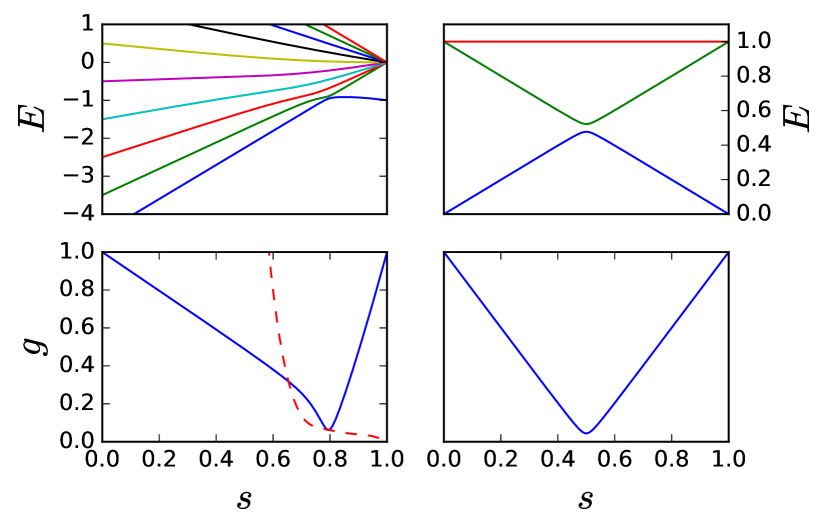
Figure 1: (color online) (Top) Energy levels and (bottom) gap for a hypercube of size $n=9$ (left) and complete graph (right). Both the true gap (blue, solid) and the approximate, analytical, gap (red, dashed) are shown for the hypercube (bottom left). The analytical gap is only accurate near the true minimum gap, however it is here that transitions to higher energy levels are most rapid, so the resulting analytical schedule still yields optimal quantum speedup. Energy units defined by Eq. (14).

The energy levels of $\hat{H}^{(h)}_{\text{AQC}}$ are shown in Fig. 1 (top left) for $n=9$, and for comparison the energy levels of the search Hamiltonian for the complete graph (which is the same for any size) are shown top right.

We also solve Eq. (16) numerically to obtain $s^{(n)}$ using an explicit numerical calculation of the gap $g(t)$, and using the maximum value of $\langle d\hat{H}^{(h)}_{\text{AQC}}/dt\rangle_{0,1}$, which is shown in appendix A to be $n/4$. Our numerical algorithm is described in appendix B. While it does not provide a closed form solution, results using $s^{(n)}$ do provide insight on the accuracy of $s^{(c)}$. Provided the numerics are performed to a sufficient accuracy, $s^{(n)}$ will always provide an optimal $\sqrt{N}$ speed up. The analytically and numerically calculated gaps are plotted in Fig. 1 (bottom left) for $n=9$, and the corresponding gap for the complete graph is shown bottom right. For the hypercube, the analytical and numerical gaps are strikingly different, yet both produce schedules that obtain a quantum speed up. As we will see, this is because for the quantum search problem only the position and size of the gap are important. Elsewhere, the transition probabilities are so small it does not matter how fast the schedule proceeds.

However, note that both of these schedules assume a two-level approximation, as they start from Eq. (16). While in general for large $N$ this is a good approximation, for small system sizes the higher energy levels do affect the performance, as we show in the next subsection.

III.3 Performance of hypercube schedules

Having calculated optimal schedules both analytically and numerically, we now compare their performance for system sizes up to $n=20$ qubits. Note that the size of the minimum gap $g_{(\text{min})}$ calculated from the two-level approximation in Sec. III is exactly the same for both. Since both are based only on the interactions of the two lowest energy levels, both will find the correct shape for the annealing protocol in this region. Numerical results support this prediction in that for $n=20$ the numerically calculated optimal schedule $s^{(n)}$ slows down at the same value as $s^{(c)}$ in Fig. 2. For $n=5$ qubits the schedules are distinct over the whole range of $\tau$, while for $n=20$, the schedules are almost identical, the only visible difference occurs at $\tau\lesssim 0.1$. The difference between them around $\tau\lesssim 0.1$ is likely due to interactions with the higher excited states of the hypercube Hamiltonian early in the schedule. In the large system limit this difference will have little effect on the overall success probability, as the overlap with the initial ground state and the manifold of states participating in the avoided crossing approaches one exponentially fast in the number of qubits $n$ (see table 1).

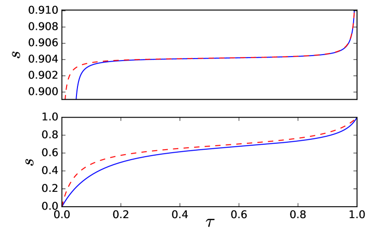
Figure 2: (color online) Comparison of annealing schedules from Sec. III for AQC searching over a hypercube of $n=20$ qubits (top) and $n=5$ qubits (bottom) for two-level approximation analytically calculated $s^{(c)}$ (dashed) and numerically calculated $s^{(n)}$ (solid). Note different scale for $s$ in top figure.

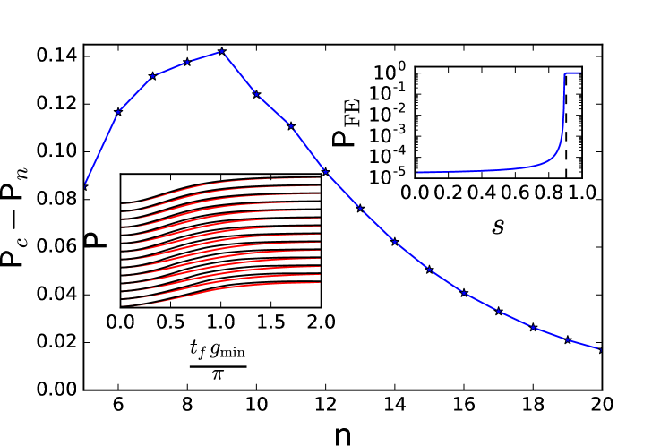
Figure 3: (color online) Main figure: Difference in success probabilities $\mathsf{P}_{c}-\mathsf{P}_{n}$ between the annealing schedule calculated analytically $s^{(c)}$ and the numerically calculated schedule $s^{(n)}$ for a single run over a time $\pi/g_{\text{min}}$. Lower Inset: Offset plot of the success probabilities $\mathsf{P}$ versus $t_{f}g_{\text{min}}/\pi$ for $s^{(c)}$ (red, gray in print) and $s^{(n)}$ (black) for $n=5$ to $n=20$. Upper Inset: Sum of the overlaps of $|E_{1}\rangle$ with $|m\rangle$ and $|\psi_{\text{init}}\rangle$ ($\mathsf{P}_{\mathrm{FE}}=|\left\langle E_{1}|m\right\rangle|^{2}+|\left\langle E_{1}|\psi_{\text{init}}\right\rangle|^{2}$) against $s$ for $20$ qubits. Since the relevant avoided crossing is in the space spanned by $|m\rangle$ and $|\psi_{\text{init}}\rangle$ a vanishing value $\mathsf{P}_{\mathrm{FE}}$ is indicative of very little rotation of the ground state. Vertical dashed line is position of $g_{\text{min}}$.

For $n<20$, the difference between $s^{(c)}$ and $s^{(n)}$ at early times in the run does affect their relative performance, as Fig. 3 shows. Although the numerical schedule $s^{(n)}$ is a more accurate solution of the optimization in Eqn. (16), $s^{(c)}$ does better than $s^{(n)}$. The reason is that, while the gap is relatively small early in the schedule, so is the matrix element between the ground and first excited state of the marked state Hamiltonian, as shown in the top inset of Fig. 3. As a result, the numerically calculated schedule slows down unnecessarily in this region, as can be seen in Fig. 2. The approximate expansion for the gap used to derive the schedule $s^{(c)}$ in appendix A grows within this region, see Fig. 1. Hence, $s^{(c)}$ traverses this part of the schedule much faster than $s^{(n)}$. Effectively, the approximate nature of the expansion for the gap used to calculate $s^{(c)}$ partially cancels an unnecessary slowdown caused by the approximation that $\langle\frac{dH}{ds}\rangle_{0,1}$ is constant for all $s$. However, as the main figure and lower inset of Fig. 3 show, the difference between the success probabilities using the two schedules shrinks as system size increases and the avoided crossing becomes more dominant.

IV Hybrid annealing schedules

Having arrived at a common Hamiltonian form for QW and AQC searching on an $n$-dimensional hypercube, and having derived optimal coefficients for each case, we can now interpolate the coefficients to generate hybrid search algorithms. In this section we show how this may be done, and study the resulting dynamics. We begin by looking at small systems with $n=5$ and $n=8$, and then study the dynamics of systems with very large $n$ by demonstrating that this limit corresponds to a two-state single avoided crossing model.

IV.1 Motivation and definition

We have already noted that QW and AQC search algorithms both use the same terms in the Hamiltonian, differing only in the time dependence. With appropriate choice of parameters, both provide a quadratic quantum speed up: a search time proportional to $\sqrt{N}$ for a search space of size $N$. This suggests the question of whether we can map smoothly between QW and AQC searching, while maintaining the quantum speed up.

To construct the mapping, we generalize the AQC Hamiltonian of Eq. (11) by defining a time-dependent Hamiltonian

$$\hat{H}(\tau)=A(\tau)\hat{H}_{0}+B(\tau)\hat{H}_{p}$$ (25)

as a function of the reduced time $\tau=t/t_{f}$, where the annealing schedules $A(\tau)$, $B(\tau)$ satisfy $A(0)\gg B(0)$ and $B(1)\gg A(1)$. The AQC algorithm as described by Eq. (11) is obtained by setting

$$A_{\text{AQC}}(\tau) =1-s(\tau)$$

$$B_{\text{AQC}}(\tau) =s(\tau).$$ (26)

The QW search Hamiltonian with hopping rate $\gamma$, described by Eq (9), can also be obtained by setting

$$A^{(\gamma)}_{\text{QW}}(\tau) =\begin{cases}\gamma&\tau<1\\ 0&\tau=1\end{cases}$$

$$B^{(\gamma)}_{\text{QW}}(\tau) =\begin{cases}1&\tau>0\\ 0&\tau=0.\end{cases}$$ (27)

We can make this even closer to the AQC form by defining $\beta=1/(1+\gamma)$ and setting

$$A_{\text{QW}}(\tau) =\begin{cases}1-\beta&\tau<1\\ 0&\tau=1\end{cases}$$

$$B_{\text{QW}}(\tau) =\begin{cases}\beta&\tau>0\\ 0&\tau=0.\end{cases}$$ (28)

For QW search on the hypercube, using Eq. (10) for $\gamma^{(h)}_{o}$, to achieve optimal $\sqrt{N}$ scaling we must set $\beta$ equal to

$$\beta^{(h)}_{o}=\frac{1}{1+R_{1}}.$$ (29)

For $0<\tau<1$, the re-parameterization of Eq. (27) in Eq. (28) maintains the ratio of $A_{\text{QW}}(\tau)/B_{\text{QW}}(\tau)=\gamma$. However, it also introduces a global energy shift $A_{\text{QW}}(\tau)=\beta A^{(\gamma)}_{\text{QW}}(\tau)$ and $B_{\text{QW}}(\tau)=\beta B^{(\gamma)}_{\text{QW}}(\tau)$. The observant reader will note that, because the optimal $\gamma^{(h)}_{o}$ is dependent on the size of the system, this re-parameterization introduces a weak dependence of the global energy scale on system size $N=2^{n}$. However, since $\beta^{(h)}_{o}\rightarrow 1$ in the large $N$ limit, this weak dependence cannot affect the leading order term in the asymptotic scaling, and the re-parameterized quantum walk search algorithm still provides optimal $\sqrt{N}$ scaling.

In the way we have parameterized them above, the AQC and QW protocols differ only in the annealing schedules $A(\tau)$ and $B(\tau)$. Hence, we can use the QW and AQC schedules as end-points of a smooth interpolation between these two search algorithms to define a continuum of hybrid protocols. Using a parameter $\alpha\in[0,1]$, where $\alpha=0$ corresponds to QW and $\alpha=1$ corresponds to AQC, we can define

$$A(\alpha,\beta,\tau) =\frac{1-s(\tau)}{\alpha+(1-\alpha)\frac{(1-s(\tau))}{(1-\beta)}}$$

$$B(\alpha,\beta,\tau) =\frac{s(\tau)}{\alpha+(1-\alpha)\frac{s(\tau)}{\beta}}.$$ (30)

giving a family of hybrid quantum algorithms defined by the Hamiltonian

$$\hat{H}_{\text{AB}}=A(\alpha,\beta,\tau)\hat{H}_{0}+B(\alpha,\beta,\tau)\hat{H}_{p}.$$ (31)

This interpolation is quite general, for well-behaved $\hat{H}_{0}$ and $\hat{H}_{p}$, with the caveat about the extra dependence of the energy scale on the QW hopping rate through $\beta$ mentioned above. The resulting family of functions is illustrated in Fig. 4 for search over $5$- and $8$-qubit hypercube graphs.

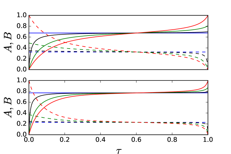
Figure 4: (color online) Interpolated schedule functions $A(\alpha,\beta,\tau)$ (dashed lines) and $B(\alpha,\beta,\tau)$ (solid lines) as defined by Eq. (IV.1) for hybrid QW-AQC quantum searching on an $n=5$ (top) and $n=8$ (bottom) dimensional hypercube graph. $\alpha=0$ (QW), blue (dark gray in print); $\alpha=0.1$, black; $\alpha=0.5$, green (mid gray in print); and $\alpha=1$ (AQC), red (light gray in print), calculated numerically following the method in Appendix B.

Note that, although it is plausible, it doesn’t follow a priori from the construction that these interpolated AQC-QW schedules will yield a quantum speed up at all for searching, let alone an optimal $\sqrt{N}$ scaling. This is because the different mechanisms in QW and AQC could be incompatible in combination. We return to this important question in Sec. IV.3, where we show that properly specified interpolations can indeed achieve the theoretical optimum $\sqrt{N}$ scaling.

IV.2 Small size examples

To gain intuition for how our interpolated schedules behave, we study small systems of five and eight qubits. These have been simulated using the full Hamiltonian on the hypercube; for numerical methods, see appendix B. Fig. 5 shows how the final success probability varies with the search duration $t_{f}$ for QW, AQC and an intermediate $\alpha=0.5$ search over the $5$-qubit hypercube graph. Note that, because the schedules $A$ and $B$ are in general nonlinear functions of time, in all plots against $t_{f}$ each point represents a separate run of the quantum search algorithm for that value of $t_{f}$; the plots do not also represent the time evolution $0\leq t\leq t_{f}$, except for $\alpha=0$ when the schedule functions are constant ($A=1-\beta$ and $B=\beta$). Plots of the time evolution for a single search can be seen in Ref. Morley et al. (2018) and in Sec. V.3. Also plotted in Fig. 5 are the annealing schedules $A$ and $B$ as a function of the reduced time $\tau$, illustrating how the shape of the functions $A(\alpha,\tau)$ and $B(\alpha,\tau)$ changes for different values of $\alpha$, from flat for a quantum walk to a curving AQC annealing schedule for $\alpha=1$.

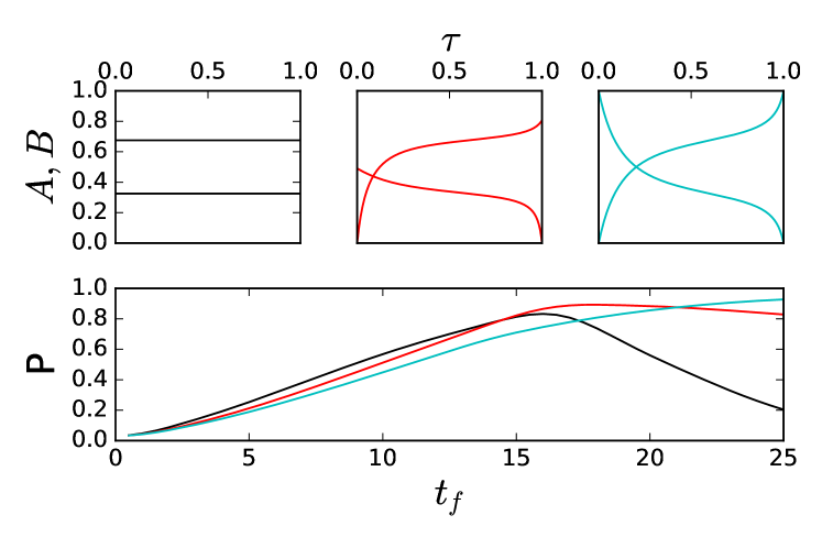
Figure 5: (color online) (Top) Numerically calculated hybrid schedules $A$ and $B$ against runtime $\tau$ for quantum search on a 5-qubit hypercube graph for $\alpha=0$ QW, (black, top left), $\alpha=0.5$ (red, mid gray in print, top middle), and $\alpha=1$ AQC, (cyan, light gray in print, top right). (Bottom) Success probability of the corresponding searches (indicated by matching colour/shade of gray in print) against total search time $t_{f}$, in units given by Eq. (25). Note that this does not show time evolution against $t$ or $\tau$.

We see that the qualitative behaviour of adiabatic evolution is fundamentally different from that of the quantum walk search. For the optimal AQC schedule the success probability increases monotonically to a value very close to one. In contrast, QW shows oscillatory behaviour, and although the success probability does not approach one, it does show a faster initial increase than for AQC. The intermediate schedule shows a mix of both behaviours, with a locally oscillating but globally increasing success probability that shows an initial increase rate between that of QW and AQC.

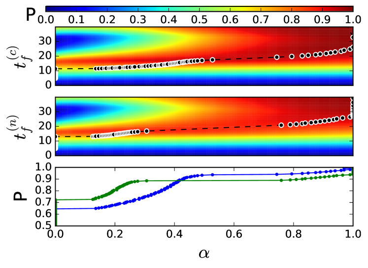
Figure 6: (color online) Successs probabilities $\mathsf{P}$ of hybrid QW-AQC quantum search on a 5-qubit hypercube graph plotted against the interpolation parameter $\alpha$ and total runtime $t_{f}$ using optimal schedules (top) $s^{(c)}$ analytical, and (middle) $s^{(n)}$ from numerical solution. Dotted lines with black points indicate the optimal protocol at a given runtime $t_{f}$. Probability corresponding to the optimal protocol (bottom) for analytical (blue, dark gray in print) and numerical (green, mid gray in print). Time units given by Eq. (25).

We now turn to the probability $\mathsf{P}$ of finding the marked state that is obtained for different choices of $\alpha$ and $t_{f}$. For a continuum of $\alpha$ values, Figs. 6 and 7 illustrate the same qualitative behaviour for 5-qubit and 8-qubit quantum searches. The oscillatory behaviour associated with a QW slowly fades away as the interpolation approaches the respective AQC schedule, at which point the success probability $\mathsf{P}$ increases monotonically with $t_{f}$. If a relatively low success probability is sufficient, only a short total runtime $t_{f}$ is needed, and quantum walk is the best strategy. As $t_{f}$ is increased, the best strategy is to increase $\alpha$ and start adding some adiabatic character into the protocol. Finally, if a high success probability is required and a long runtime $t_{f}$ is possible, then AQC becomes the best strategy. We also see that, for these system sizes, the hybrid protocols maintain the quantum speed up for the search algorithm runtime.

We now consider the differences between the calculated and numerical annealing schedules $s^{(c)}$ and $s^{(n)}$ for these small systems. Fig. 6 depicts results for $n=5$ qubits. The main difference for five qubits is that the numerically calculated optimal schedule $s^{(n)}$ is able to perform substantially better for $\alpha<0.4$, where “better” means a higher probability of success for a given runtime $t_{f}$ and value of $\alpha$.

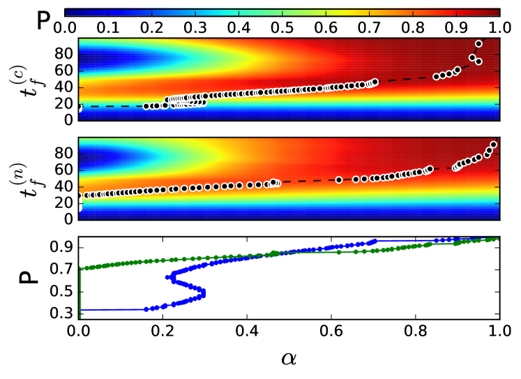
Figure 7: (color online) Successs probabilities $\mathsf{P}$ of hybrid QW-AQC quantum search on an 8-qubit hypercube graph plotted against the interpolation parameter $\alpha$ and total runtime $t_{f}$ using optimal schedules (top) $s^{(c)}$ analytical, and (middle) $s^{(n)}$ from numerical solution. Dotted lines with black points indicate the optimal protocol at a given runtime $t_{f}$. Probability corresponding to the optimal protocol (bottom) for analytical (blue, dark gray in print) and numerical (green, mid gray in print). Time units given by Eq. (25).

Figure 7 shows the same comparisons for the slightly larger value of $n=8$ qubits. The optimal $\alpha$ moves away from $\alpha=0$ at a smaller value of $t_{f}$ and $\mathsf{P}$ for $s^{(c)}$ than it does for $s^{(n)}$. There is also more structure in the optimal $\alpha$ line (black dashes) for $s^{(c)}$ than for $s^{(n)}$, with a range of $\alpha$ values that are optimal for more than one value of $\mathsf{P}$. Otherwise, the two behave quite similarly for these small sizes, suggesting that both $s^{(c)}$ and $s^{(n)}$ are able to provide a quantum speed up for hybrid protocols. To confirm this in general, not just for small $n$, further analysis and simulations of larger systems are required, which we tackle in the following subsections.

IV.3 Performance of hybrid algorithms

Our strategy for analyzing the scaling of the hybrid quantum search algorithms is to show that the performance is dominated by a single, low energy, avoided crossing, see Fig. 1, which is present at the same position in all our hybrid algorithms. We then show that the essential features of the behavior are captured by a simple, two-state single avoided crossing model which all the hybrid algorithms map to in the large size limit. For this simple avoided crossing model we can easily show that the hybrid algorithms all provide an optimal quantum speed up. It then follows that our full-size hybrid algorithms have the same asymptotic scaling.

We first consider the end points of the interpolation, QW and AQC search. For AQC search, the optimal schedule $s^{(c)}(\tau)$ or $s^{(n)}(\tau)$ is derived directly from the functional form of the lowest avoided crossing, ensuring that the Hamiltonian is changed slowly enough to avoid transitions to higher energy levels. We only need to show that the low energy structure of the Hamiltonian is dominated by a single avoided crossing throughout the process. This is shown numerically in Fig. 8. The width $w(n)$ of the avoided crossing decreases rapidly with $n$. Even for a modest size of $n=50$ qubits, the switch from $95\%$ overlap with the hypercube Hamiltonian ground state to $95\%$ overlap with the marked state occurs in less than $10^{-6}$ of the total dynamic range of the protocol, which runs from $s(\tau)=0$ to $s(\tau)=1$.

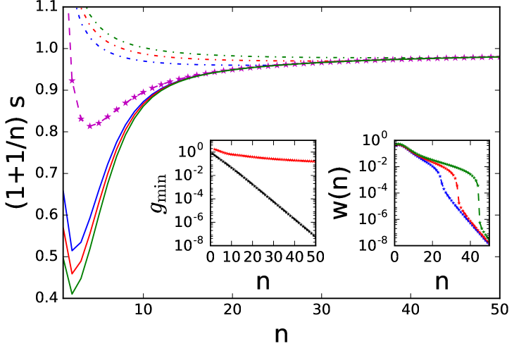
Figure 8: (color online) Main figure: $s(\tau)$ scaled by $(1+1/n)$ against number of qubits $n$ for $90\%$ (blue, dark gray in print), $93\%$ (red, light gray in print), $95\%$ (green, mid gray in print) overlap of $|\psi(t)\rangle$ with $|m\rangle$ (solid) and with $|\psi_{\text{init}}\rangle$ (dot-dashed). Magenta stars are the transition point, the value of $s(\tau)$ when the minimum gap $g_{\text{min}}$ occurs. Left inset: $g_{\text{min}}=\min(E_{1}-E_{0})$ (lower black stars) and $\min(E_{2}-E_{0})$ (upper red stars, light gray in print). Energy units given by Eq. (25). Right inset: width of the transition $w(n)=\Delta s(\tau)$, the difference between solid and dot-dashed curves of the same color in the main figure. Calculated using the AQC search hypercube Hamiltonian mapped to the line, see Appendix B.

In contrast, for QW search, transitions to higher energy levels are a necessary part of the evolution to the marked state, so we need to determine the scaling of several related quantities to show that a single avoided crossing dominates in determining the behavior.

IV.4 Minimum gap scaling in QW search

For QW search, to show numerically that the lowest avoided crossing is the only relevant feature in the large $N$ limit, we must demonstrate two things. First, that the minimum gap $g_{\text{min}}=(E_{1}-E_{0})$ between the ground state and the first excited state becomes much smaller than the minimum gap between the ground state and the second excited state. Second, that the lowest avoided level crossing, where $g(\tau)=g_{\text{min}}$, dominates the transition between the ground state of the hypercube Hamiltonian $\hat{H}^{(h)}_{0}$ and the ground state of the marked state Hamiltonian $\hat{H}_{\textsc{p}}$, and becomes more dominant as system size increases. Noting that, as illustrated in Fig. 4, around the minimum gap, where all the schedules cross, we have $(1-s(\tau))\simeq\gamma^{(h)}_{o}$, Figure 8 shows that both of these do, in fact, occur. The left inset shows that at the avoided crossing, the gap between the ground state and first excited state shrinks exponentially faster in $n$ than the gap between the ground state and second excited state. The main figure and right inset of Fig. 8 show how the transition between the two ground states becomes dominated by the dynamics at $g_{\text{min}}$ as $n$ increases.

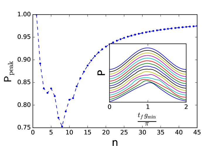
Figure 9: (color online) Main figure: Search success probability $\mathsf{P}$ at the first peak for a quantum walk search against qubit number $n$ up to $n=50$. Inset: Rescaled offset plot of $\mathsf{P}$ against $t$ starting at the bottom with $n=5$ qubits and going to $n=20$. Calculated using the hypercube QW search mapped to the line.

For a pure quantum walk search, this convergence to behaviour dominated by a single avoided crossing can be seen in Fig. 9, which shows that not only does the search success probability $\mathsf{P}$ approach one in the large system limit (main figure), but also that the time evolution of $\mathsf{P}$ (inset) approaches the functional form for the single avoided crossing $\mathsf{P}(\tau)=\sin^{2}(g_{\text{min}}t_{f}/2)$. The non sinusoidal shapes of these curves at low qubit number are due to the influence of excited states higher than the first exited state. In the main figure, these small size effects are clearly significant up to about $n=12$ qubits. This highlights the potentially atypical nature of the 5- and 8-qubit examples in Sec. IV.2, and the importance of examining larger system sizes. For $n>12$, the probability $\mathsf{P}$ smoothly approaches one, although relatively slowly (polynomially) as a function of $n$. Based on the data in table 1 we can deduce that this effect relates to the fact that the overlap of the manifold where the avoided crossing takes place with the marked state only approaches one polynomially in $n$ (logarithmically in $N$).

Since states of higher energy than the first excited state play very little role in the QW search dynamics for larger systems, we can approximate the probability that the marked state can be reached using only the manifold $\mathcal{T}=\{|E_{0}\rangle,|E_{1}\rangle\}$ of ground and first excited states of the full search Hamiltonian $\hat{H}^{(h)}_{\text{QWS}}$. This can be upper bounded by considering the probability that the dynamics transfers as much as possible of $|\psi_{\text{init}}\rangle$ into $\mathcal{T}$, and then optimally aligns the system state with $|m\rangle$ without leaving $\mathcal{T}$. Using $\hat{\mathcal{P}}_{\mathcal{T}}=|E_{0}\rangle\langle E_{0}|+|E_{1}\rangle\langle E_{1}|$, the projector onto $\mathcal{T}$, this can be shown to be given by the product of the sums of the overlaps,

$$\mathsf{P}_{\max}^{\text{(}QW)} =|\hat{\mathcal{P}}_{\mathcal{T}}|\psi_{\text{init}}\rangle|^{2}\times|\hat{\mathcal{P}}_{\mathcal{T}}|m\rangle|^{2}$$

$$=\left(|\left\langle\psi_{\text{init}}|E_{0}\right\rangle|^{2}+|\left\langle\psi_{\text{init}}|E_{1}\right\rangle|^{2}\right)$$

$$\times\left(|\left\langle E_{0}|m\right\rangle|^{2}+|\left\langle E_{1}|m\right\rangle|^{2}\right),$$ (32)

when single avoided crossing behaviour dominates.

Quantity	Scaling	$1-r^{2}$
$\mathsf{P}_{\max}^{\text{(}QW)}$	$1-1.734\times n^{-1.112}$	$7.820\times 10^{-5}$
$|\left\langle E_{0}|m\right\rangle|^{2}+|\left\langle E_{1}|m\right\rangle|^{2}$	$1-1.734\times n^{-1.112}$	$7.820\times 10^{-5}$
$|\left\langle\psi_{\text{init}}|E_{0}\right\rangle|^{2}+|\left\langle\psi_{\text{init}}|E_{1}\right\rangle|^{2}$	$1-4.292\times 2^{-1.186\,n}$	$0.00143$
$\gamma^{(h)}_{o}$	$1-1.233\times n^{-1.0425}$	$1.120\times 10^{-5}$

Table 1: Numerical fits for various quantities related to quantum walks and adiabatic protocols. These fits were performed using linear fitting on either logarithmic or semi-logrithmic axes in the range $n=40$ to $n=70$, except for $|\left\langle\psi_{\text{init}}|E_{0}\right\rangle|^{2}+|\left\langle\psi_{\text{init}}|E_{1}\right\rangle|^{2}$ which was fit over the range $n=11$ to $n=40$ due to numerical precision issues. The coefficient of determination $r^{2}\equiv 1-\frac{\sum_{i}(y_{i}-f_{i})^{2}}{\sum_{i}(y_{i}-\bar{y})^{2}}$, where $f_{i}$ are the data and $y$ is the fitting function, is calculated against the linear function on the logarithmic or semi-logarithmic axes. These fits are plotted along with the data used to produce them in Fig. 10. The slight difference from $-1$ in the scaling exponent for $\gamma^{(h)}_{o}$ is due to numerical finite size effects.

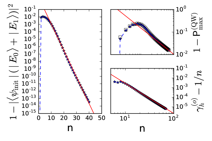
Figure 10: (color online) Scaling of various quantities related to QW searching. Left: difference from one of the overlap of $|\psi_{\text{init}}\rangle$ with $|E_{0}\rangle$ and $|E_{1}\rangle$ against number of qubits $n$. Top Right: difference from one of marked state with $|E_{0}\rangle$ and $|E_{1}\rangle$ (stars) and $\mathsf{P}_{\max}^{\text{(}QWS)}$ (squares), against $n$. Bottom right $\gamma^{(h)}_{o}-1/n$ versus $n$. Solid lines (red online) are numerical fits, summarized in table 1. Calculated using the hypercube QW search mapped to the line.

Figure 10 shows how $\mathsf{P}_{\max}^{\text{(}QW)}$ approaches one as $n$ increases, by plotting the difference from one on a log or log-log scale. The top right figure shows that $\mathsf{P}_{\max}^{\text{(}QW)}\rightarrow 1$ only happens relatively slowly, with a polynomial scaling in $n$, and therefore logarithmic in $N$. By plotting the first overlap in Eq. (IV.4) separately, the left figure shows that the overlap of $|\psi_{\text{init}}\rangle$ with $|E_{0}\rangle$ and $|E_{1}\rangle$ rapidly approaches one. Hence, the scaling of $\mathsf{P}_{\max}^{\text{(}QW)}$ shown top right is dominated by the overlap of the marked state with the lowest energy states $|E_{0}\rangle$ and $|E_{1}\rangle$ at the gap. We can quantify how slowly $\mathsf{P}$ approaches one by doing numerical fits to determine the scaling of the relevant quantities: these are summarized in table 1. In particular, we note that $\gamma^{(h)}_{o}$ only approaches $1/n$ linearly in $n$, consistent with the analytical results in Ref. Childs and Goldstone (2004).

The fact that $\mathsf{P}_{\max}^{\text{(}QW)}\rightarrow 1$ suggests that the optimal protocol for all success probabilities should approach QW ($\alpha=0$) for large system size, because QW does not slow down at the minimum gap like AQC does. However, $\mathsf{P}_{\max}^{\text{(}QW)}\rightarrow 1$ only happens relatively slowly: the maximum $\mathsf{P}_{\max}^{\text{(}QW)}$ which a QW search obtains only reaches $99\%$ by around $100$ qubits. Brute force classical techniques will become computationally non-trivial beyond around 30 bits, where $\mathsf{P}_{\max}^{\text{(}QW)}\approx 95\%$. The finite size effects we study here are thus relevant to real world applications.

IV.5 Single avoided crossing model

We have shown that a single avoided crossing dominates for large $N$ for both QW and AQC search algorithms on the hypercube. Dominance of a single avoided crossing is the method used to solve analytically for all Hamiltonian-based quantum search algorithms treated to date, including the complete graph Roland and Cerf (2002) and Cartesian lattices (which provide a quantum speed up for $d\geq 4$ dimensions) Childs and Goldstone (2004). It is also the typical behavior for a broad class of random search graphs Chakraborty et al. (2016). We now introduce a simple, two state, single avoided crossing model for quantum search which provides the quadratic quantum speed up. We will then show how all of our hybrid protocols can be mapped onto it.

There are several ways to parameterize a two-state single avoided crossing model. If we designate the marked state to be the $|0\rangle$ state of a qubit, this will be the end point of the schedule. The initial state needs to be orthogonal to $|0\rangle$, i.e., it has to be $|1\rangle$. These two states are the lowest energy eigenstates of $\frac{1}{2}(\openone+\hat{\sigma}_{z})$ and $\frac{1}{2}(\openone-\hat{\sigma}_{z})$ respectively, where the factor of $\frac{1}{2}$ makes the eigenenergies zero and one in our units. We also need a hopping Hamiltonian term $\hat{\sigma}_{x}$, to drive transitions between $|1\rangle$ and $|0\rangle$. The relative strength of the hopping Hamiltonian is $g_{\text{min}}$, the minimum gap at the avoided crossing. The single avoided crossing AQC search Hamiltonian is

$$\hat{H}^{(\text{AC})}(s) =(1-s)\hat{H}^{\text{(AC)}}_{0}+s\hat{H}^{\text{(AC)}}_{p}$$

$$=(1-s)\left\{\frac{1}{2}(\openone+\hat{\sigma}_{z})-g_{\text{min}}\hat{\sigma}_{x}\right\}+s\frac{1}{2}(\openone-\hat{\sigma}_{z}).$$ (33)

The initial state $|1\rangle$ is only an approximate eigenstate of $\hat{H}^{\text{(AC)}}_{0}$ but the approximation improves as $g_{\text{min}}$ decreases. Solving the eigensystem for this Hamiltonian gives

$$g^{(\text{AC})}(s)=\{(1-2s)^{2}+4g^{2}_{\text{min}}(1-s)^{2}\}^{\frac{1}{2}}$$ (34)

for the gap between the two energy levels. In the limit of small $g_{\text{min}}$ the minimum gap is $g_{\text{min}}$ and occurs for $s=\frac{1}{2}$. We can then apply the method of Roland and Cerf (2002) to find the optimal schedule $s(t)$ for this system. Calculating $d\hat{H}/ds$ we find

$$\frac{d\hat{H}}{ds}^{(\text{AC})}=-\hat{\sigma}_{z}+g_{\text{min}}\hat{\sigma}_{x}$$ (35)

giving a maximum value of one for $|\langle\frac{d\hat{H}^{(\text{AC}})}{ds}\rangle_{0,1}|$ in the large-size limit. Using Eq. (20) to find the optimal schedule, we need to solve

$$\frac{ds}{dt}=\frac{\epsilon[g^{(\text{AC})}(s)]^{2}}{|\langle\frac{d\hat{H}_{\text{AC}}}{ds}\rangle_{0,1}|}=\epsilon\{(1-2s)^{2}+4g^{2}_{\text{min}}(1-s)^{2}\},$$ (36)

where the maximum value is used for $|\langle\frac{d\hat{H}^{(\text{AC}})}{ds}\rangle_{0,1}|$. This can be integrated straightforwardly to give

$$\arctan\left\{2g_{\text{min}}(s-1)+\frac{2s-1}{g_{\text{min}}}\right\}=2g_{\text{min}}\epsilon t+c$$ (37)

with

$$c=-\arctan\left\{2g_{\text{min}}+\frac{1}{g_{\text{min}}}\right\}.$$ (38)

From this we find for $s=1$ that the runtime $t_{f}^{(AC)}$ is given by

$$\epsilon\,t_{f}^{(AC)}=\frac{\frac{\pi}{2}-\arctan(g_{\text{min}})}{g_{\text{min}}}\simeq\frac{\pi}{2\,g_{\text{min}}}-1,$$ (39)

where the approximate expression uses $\arctan(1/g_{\text{min}})\simeq\frac{\pi}{2}-g_{\text{min}}$ for $g_{\text{min}}\ll 1$ and terms of order $g^{2}_{\text{min}}$ have been dropped. The runtime of the optimal schedule thus depends inversely on the size of the minimum gap, as expected. Solving for $s(t)$ and dropping terms of order $g^{2}_{\text{min}}$ gives

$$s(t)\simeq\frac{1}{2}\left\{1-g_{\text{min}}\cot\left[g_{\text{min}}(2\epsilon t+1)\right]\right\}.$$ (40)

In this limit where $g_{\text{min}}\ll 1$, an equivalent way to parameterize $\hat{H}^{(\text{AC})}$ is

$$\hat{H}^{(\text{AC})}=\frac{g_{\text{min}}}{2}\left[f(t)\hat{\sigma}_{z}-\hat{\sigma}_{x}\right],$$ (41)

where $-\infty<f(t)<\infty$. This form is obtained by taking $(1-2s(t))/g_{\text{min}}\rightarrow f(t)$ and shifting the zero point of the energy scale to the middle of the avoided crossing. As $f(t)$ changes from $-\infty$ to $\infty$ it passes through zero as the sign of the $\hat{\sigma}_{z}$ term changes, when the $\hat{\sigma}_{x}$ term drives the transition from $|1\rangle$ to $|0\rangle$. Although the $\hat{\sigma}_{x}$ term is no longer turned off at the end of the schedule, it becomes negligible in comparison to the $\hat{\sigma}_{z}$ term and does not significantly alter the dynamics. This can be intuitively thought of as scaling all features of $\hat{H}^{(\text{AC})}$ other than the avoided crossing to $\pm\infty$.

The QW form of the single avoided crossing search Hamiltonian is also simple to analyze. We deduce the optimal value of $\gamma_{o}=1$ from the value of $s=\frac{1}{2}$ at the avoided crossing. We then use Eqns. (28) in which $\beta_{o}=1/(1+\gamma_{o})=\frac{1}{2}$, whence

$$\hat{H}^{\text{AC}}_{(\text{QWS})} =(1-\beta_{o})\hat{H}^{\text{(AC)}}_{0}+\beta_{o}\hat{H}^{\text{(AC)}}_{p}$$

$$=\frac{1}{2}\left\{\frac{1}{2}(\openone+\hat{\sigma}_{z})-g_{\text{min}}\hat{\sigma}_{x}+\frac{1}{2}(\openone-\hat{\sigma}_{z})\right\}$$

$$=\frac{1}{2}(\openone-g_{\text{min}}\hat{\sigma}_{x})$$ (42)

The $\hat{\sigma}_{x}$ term causes deterministic transitions between the two states regardless of their energies, at a rate determined by $g_{\text{min}}$. By solving for the dynamics, the time for the input state $|1\rangle$ to evolve to the marked state $|0\rangle$ can be shown to be $t_{f}^{(qw)}=\pi/g_{\text{min}}$.

We can now map between QW and AQC in the avoided crossing model using Eqs. (IV.1) for $A(\alpha,\beta,\tau)$ and $B(\alpha,\beta,\tau)$. Using $\beta=\frac{1}{2}=1/(1+\gamma_{o})$, for $s(t)$ from Eq. (40) we have hybrid schedules

$$A_{\text{AC}}(\alpha,t) =\frac{1-s(t)}{\alpha+2(1-\alpha)(1-s(t))}$$

$$B_{\text{AC}}(\alpha,t) =\frac{s(t)}{\alpha+2(1-\alpha)s(t)}.$$ (43)

We can easily show numerically that all the hybrid algorithms defined by Eqs. (IV.5) find the marked state with high probability (given by $\epsilon$) in a runtime $\lesssim\epsilon t_{f}^{(AC)}$ given by Eqn. (39), the runtime required by the optimal AQC $s(t)$ used to define the hybrid schedules. Figure 11 shows this is indeed the case. The white contours highlight the difference between the pure QW search, which succeeds with certainty, and the AQC and hybrid algorithms, which always have a probability of error $\epsilon^{2}$ that can be traded against the runtime $t_{f}$. The shallow upward curve of these contours towards the AQC end of the hybrid protocols shows in what sense the QW search is better than AQC in the large size limit.

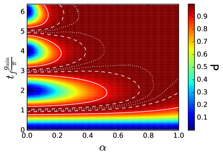
Figure 11: Probability $\mathsf{P}$ of finding the marked state versus runtime $t_{f}$ and interpolation parameter $\alpha$ for the single avoided crossing model. White contours show solid=0.9, dashed=0.99, dotted=0.999 success probability $\mathsf{P}$.

The hybrid algorithms on the full hypercube map onto the hybrid single avoided crossing model algorithms for large $n$. This follows from the solution methods for the end points, QW and AQC searching, which all use the two-level approximation to prove the quadratic speed up. Since the full hypercube hybrid algorithms are defined from these in the same way as the single avoided crossing model hybrid algorithms are defined, the hybrid algorithms also map to the corresponding single avoided crossing hybrid algorithm. They therefore also obtain the quantum speed up for large $n$, which is what we set out to show.

IV.6 Optimal hybrid algorithm for a single run

Having shown that hybrid protocols between QW and AQC maintain the quadratic quantum speed up, the next question is how to optimize over this continuum of hybrid schedules for finite size systems. The single avoided crossing model gives the large size limit in which QW is the optimal strategy. However, this limit is only reached in a polynomial scaling with $n$, as described in Sec. IV.4.

For a single run of a search algorithm, we can trade off between the magnitude of the success probability and the runtime of the search. For QW searches, there is a maximum probability $\mathsf{P}_{\max}^{\text{(}QW)}$ that can be obtained; shorter runtimes reach lower success probabilities, and so do longer runtimes. For AQC searches a longer runtime always reaches a higher success probability. We can thus specify the success probability we require and ask which hybrid algorithm attains this success probability with the shortest runtime. We consider multiple run strategies in Sec. V.

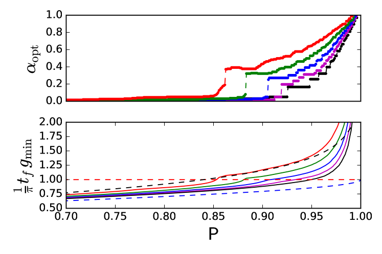
Figure 12: (color online) Top: Value of interpolation parameter $\alpha$ giving the shortest runtime for a fixed success probability $\mathsf{P}$ for a single search, using numerically calculated optimal schedules $s^{(n)}$ for hypercube dimensions (listed from top line to bottom line): $n=12$ (red); $n=14$ (green); $n=16$ (blue); $n=18$ (magenta); $n=20$ (black). Bottom: Normalized runtime versus $\mathsf{P}$ for corresponding $\alpha$ and hypercube dimension as above (solid lines, same ordering as above). Dashed lines: single avoided crossing model (large $N$ limit) for $t_{f}=g_{\text{min}}/\pi$, the time at which a QW reaches a success probability of one (red), time for QW to reach $\mathsf{P}$ (blue), time for AQC to reach $\mathsf{P}$ (black).

As Fig. 12 (top) illustrates for sizes from $n=12$ to $n=20$, the optimal protocol jumps from QW to hybrid at $\mathsf{P}\approx\mathsf{P}_{\max}^{\text{(}QW)}$, and the optimal hybrid strategy it jumps to becomes more QW-like (smaller $\alpha$) as the system size increases. As $\mathsf{P}$ is increased further, the optimal hybrid strategy becomes steadily more AQC-like (larger $\alpha$). Figure 12 (bottom) shows that the hybrid strategies require runtimes $t_{f}$ larger than $g_{\text{min}}/\pi$ to achieve higher success probabilities in a single run.

V Multiple runs for one search

In the previous sections we derived hybrid search Hamiltonians for the hypercube, and studied their dynamics. However this doesn’t yet give us a full picture of the relative usefulness of the different dynamics. In this section we study the relative performance of the different searches when we allow for the possibility of multiple searches, and when the system suffers from decohering interactions with its environment.

V.1 Motivation

In a realistic setting of the search problem we can easily check whether the result of a search is the correct answer or not. Hence, we must consider not only single run strategies, but also multi-run strategies, where the success probability is defined as the probability of succeeding in at least one of several runs. In the context of quantum search on the hypercube, we measure which site of the hypercube our state is on, and then determine the energy of this state with respect to the search Hamiltonian. If this energy is zero, then we have found the state we are looking for, otherwise, we should re-initialize and run the search again. However, we also need to account for a non-zero ‘initialization’ time $t_{\text{init}}$ associated with each run of the search. Such an initialization time is mathematically as well as physically necessary. The fidelity between the initial state and marked state $|\left\langle\psi_{\text{init}}|m\right\rangle|^{2}=\frac{1}{N}$ is non-zero. An arbitrarily short run is equivalent to making a random guess. Therefore, without an additional penalty per run, it would be possible to guess an arbitrarily large number of times for free, thus finding the marked state in a total arbitrarily short time. Any physical device will take a significant amount of time both to setup the initial state and to measure the final state. For the purposes of our study, the effects on the total search time of initialization and readout times are the same, therefore the quantity we call $t_{\text{init}}$ should be taken to include all of the time associated with a single run other than the actual runtime of the algorithm $t_{f}$, i.e., as including both initialization and measurement.

V.2 Multiple run searching

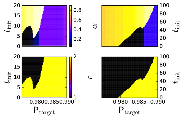
Figure 13: (color online) Optimal number of runs $r$ (bottom) and optimal $\alpha$ (top) for the numerically optimized strategy $s^{(n)}$ with $n=12$ (left) and $n=14$ (right) qubits versus $t_{\text{init}}$ and search success probability $\mathsf{P}$. $t_{\text{init}}$ is in inverse energy units, the same as $t_{f}$ on other figures.

As examples, we consider $n=12$ and $n=14$ qubits using the numerically calculated optimal strategy $s^{(n)}$. Referring to Fig. 9, $n=12$ still shows finite size effects, while $n=14$ is just into the smoothly scaling regime. We find for chosen success probabilities in the range $0.95-0.99$, the optimal strategy depends on both $t_{\text{init}}$ and $\mathsf{P}_{\text{target}}$ as shown in Fig. 13. For the range of $t_{\text{init}}$ we examine, both sizes show a transition from a single run able to reach the required success probability to a region requiring two runs. The single runs are hybrid, becoming progressively more AQC-like as the required probability increases. At the point where two runs can do better than one AQC run, the two run strategy is much closer to quantum walk, but becomes progressively more hybrid as target success probability increases further. Finite size effects are visible for $n=12$ in the non-monotonic shape of the boundary between one run and two runs in Fig. 13 (left). For smaller $n<12$, these effects become more complicated, there is no single “best strategy” for a small search space. Indeed, we also found that the optimal strategy changes significantly when any of the parameters are varied. The complexity in the optimal search strategy for small $n$ is because the two-level approximation does not hold well in this regime, and interactions with higher excited states have a non-negligible effect. This suggests that a similarly complex situation will likely be present in more sophisticated optimization Hamiltonians, whenever a two-level approximation is not valid.

V.3 Noisy quantum searching

Another realistic situation where multiple runs can be helpful is when there is a significant level of unwanted decoherence or other forms of noise acting on the quantum hardware. In this case, shorter runs that end before decoherence effects are too strong, but consequently have lower success probabilities and hence need more repeats, may be able to maintain a quantum speed up. Decoherence effects on the different AQC and QW mechanisms are analysed in more detail in related work Morley et al. (2018), and the effects of noise in AQC search have been studied in de Vega et al. (2010); Wild et al. (2016). Here we focus on hybrid algorithms, and the extra options these provide for optimizing the search.

We choose a simple model of decoherence by adding a Lindblad term to the von-Neumann equation for the system density operator $\hat{\rho}(t)$,

$$\frac{\partial\hat{\rho}(t)}{\partial t}=-\frac{i}{\hbar}[\hat{H}(t),\hat{\rho}(t)]+\kappa\mathds{P}[\hat{\rho}(t)],$$ (44)

where $\hat{H}(t)$ is the search Hamiltonian and $\kappa\mathds{P}[\rho(t)]$ is a decoherence term tuned by a rate $\kappa$. We choose a form for $\mathds{P}$ that uniformly reduces the coherences between states corresponding to vertices of the hypercube (the computational basis). This type of decoherence has been well-studied in the context of quantum walks Alagic and Russell (2005); Richter (2007); Kendon and Maloyer (2008) and, for high decoherence rate $\kappa\gg\gamma$, can be thought of as continuous measurement in the search space resulting in a quantum Zeno effect Misra and Sudarshan (1977). It is equivalent to coupling with an infinite temperature bath.

Since we now have five parameters to optimize over for a given search size $n$, ($\mathsf{P},t_{f},\alpha,\kappa$ and number of runs $r$), we first consider single run searches with success probability $\mathsf{P}(t_{f},\alpha,\kappa)$. This is the final success probability of a hybrid search specified by $\alpha$ of duration $t_{f}$ in the decoherence model of Eq. (44) with decoherence rate $\kappa$. We simulate the searches for durations $0\leq t_{f}\leq 200$, and define the search duration $t_{o}$ that maximizes $\mathsf{P}$ for a particular choice of $\alpha$ and $\kappa$. We also define $\alpha_{o}$ as the value of $\alpha$ which maximizes $\mathsf{P}(t_{o},\kappa,\alpha)$, this corresponds to the search that reaches highest success probability for a given decoherence rate $\kappa$. Note that, for computational reasons, we limited $\alpha$ to the values $0.0,0.1,0.2\dots 0.9,1.0$ when performing the maximizations; intermediate values are of course possible.

We begin by looking at how the instantaneous success probability $\mathsf{P}(t)=\left\langle m\left\lvert\rho(t)\right\rvert m\right\rangle$ evolves during a search, where $m$ denotes the marked site. Inset in Fig. 14 are plots of the evolution of $\mathsf{P}$ during a search over a $7$-qubit hypercube graph for varying decoherence rates $\kappa$, in terms of reduced time $\tau=t/t_{f}$, for a $t_{f}$ that shows the first peak of QW search. The broad effect of the decoherence is to reduce the instantaneous success probability towards a value of $1/N$, equivalent to classical guessing.

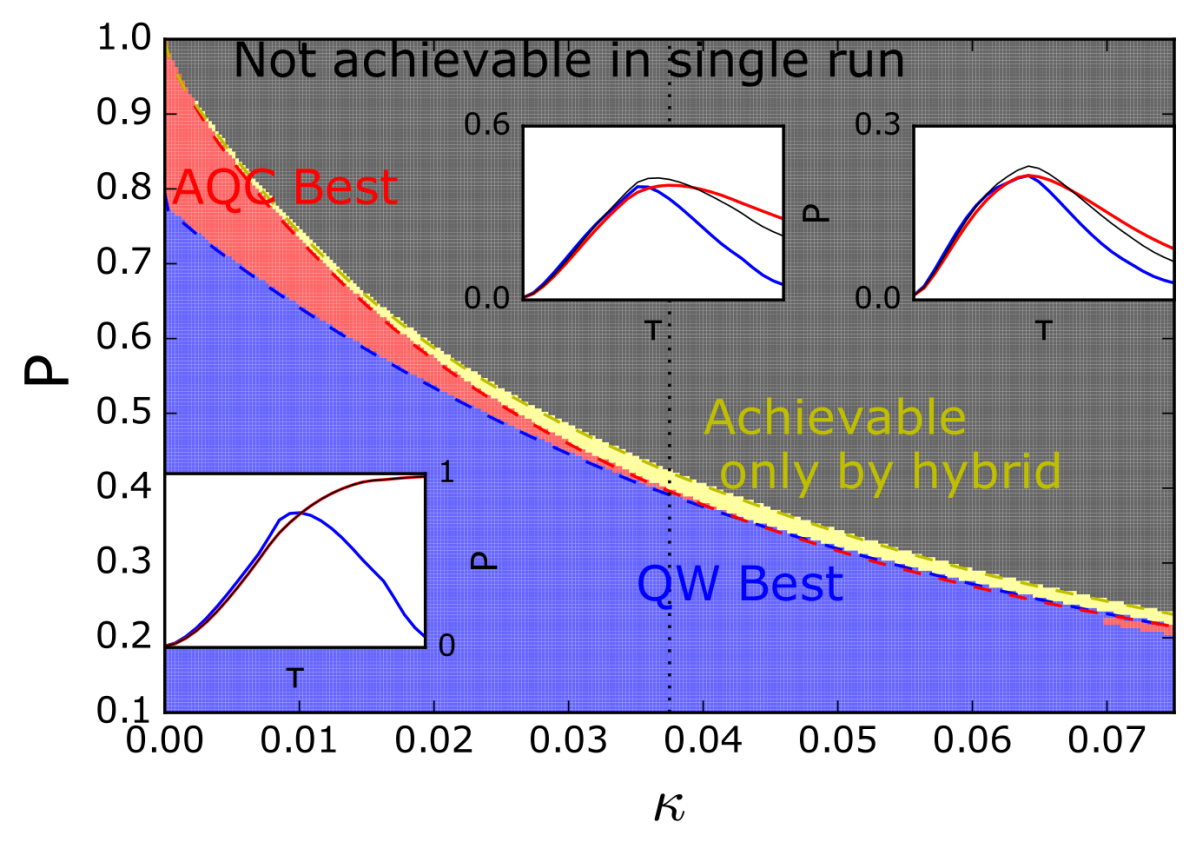
Figure 14: (color online) Main: Shaded regions show fastest protocol: QW (blue), AQC (red), hybrid advantage (yellow), and not achievable in a single run (black). Maximum success probability $\mathsf{P}$ as dashed lines in matching colours, versus decoherence rate $\kappa$, for $n=7$. Insets left to right: $\mathsf{P}$ against reduced time $\tau$ for QW (blue), AQC (red) and the optimal hybrid strategy (thin, black) for $\kappa=0$, $0.0385$ (vertical dotted line), $0.075$.

The QW, AQC and hybrid search algorithms retain their characteristics up to an overall decoherence damping, which is independent of $\alpha$. As can be seen for the $\kappa=0$ subplot (left) in Fig. 14, the QW search spreads out more quickly over the search space and therefore exhibits a more rapid initial increase in $\mathsf{P}$. On the other hand, AQC searching can reach higher values of $\mathsf{P}$ for sufficiently small values of $\kappa$, albeit at later times

The main plot in Fig. 14 shows which is fastest out of individual QW, AQC and hybrid searches for a single search, for a given value of $\kappa$ and of $\mathsf{P}$: from AQC through to hybrid when maximal success probability is required, with QW performing best for slightly lower values of $\mathsf{P}$. This indicates a remarkably large range of situations where QW dynamics is desirable - either as part of hybrid algorithms that hit the highest success probabilities for all but the smallest decoherence rates, or alone in the form of a static Hamiltonian, if a marginally smaller success probability can be tolerated.

Another way to compare the different searches under decoherence is to ask whether a QW, AQC, or hybrid search will give the maximum possible success probability $\mathsf{P}$ for a given value $\kappa$. The bottom of Fig 15 shows how this maximum $\mathsf{P}$ varies for the three cases, as well as the value of interpolation parameter $\alpha^{(o)}$ for the best-case hybrid search. For small values of $\kappa$, $\alpha_{o}=1$, i.e. AQC gives the highest peak success probability. As $\kappa$ is increased, the highest-scoring search changes and $\alpha_{o}$ decreases monotonically, indicating hybrid searches perform the best overall for intermediate levels of decoherence. In the limit of very high decoherence we are in a quantum Zeno effect regime which keeps the search in the initial superposition over all possible states. This means all searches will succeed with the same probability $\mathsf{P}=|\langle\psi_{\text{init}}|m\rangle|^{2}=1/N$, equivalent to classical guessing. The usefulness of a search is also determined by how quickly it can be performed, and so the search time $t_{f}$ is shown at the top of Fig. 15, showing that while QW never has the highest success probability in the range we examine, it can be substantially quicker. This helps to explain why hybrid schedules take on more QW character as $\kappa$ is increased, and soon begin to achieve higher success probabilities than AQC in shorter search times.

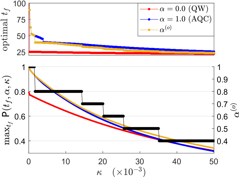
Figure 15: (color online) Quantum searching on the $n=7$ hypercube for QW (red, mid gray in print)), AQC (blue, dark gray in print), and the hybrid search which yields the maximum $\mathsf{P}$ (orange, light gray in print) given by $\alpha_{o}$. Top: search time $t_{o}$ which maximizes $\mathsf{P}$ versus $\kappa$. The first data point (not shown) for the AQC and $\alpha_{o}$ series exceeds $t_{f}=200$, the upper limit of search times sampled. Bottom: search probability $\mathsf{P}(t_{f},\alpha,\kappa)$ versus decoherence rate $\kappa$ maximized over search times $0\leq t_{f}\leq 200$ (left axis). $\alpha_{o}$ as $\kappa$ varies (black, right axis label). The $\alpha$ values sampled are $0.0,0.1,\dots,1.0$. Analytic expression (21) used for AQC schedule. Time and rate units given by Eq. (25).

Having characterized the effects of decoherence on a single run, we now consider multiple-run search strategies where each search is of the same duration $t_{f}$. We define the optimal annealing schedule as that which minimizes the time taken to reach a given success probability, optimized over all equal duration multiple-run hybrid search strategies, with durations of individual searches in the range $0<t_{f}\leq 200$. There are three variables to optimize over: the success probability $\mathsf{P}$, the initialization time between searches $t_{\text{init}}$, and the decoherence rate $\kappa$. We denote the number of runs by $r$, so the combined search time is $rt_{f}$, the combined initialization time is $rt_{\text{init}}$, and the total time taken is $r(t_{f}+t_{\text{init}})$.

To make this multiple parameter optimization tractable, we considered a discrete set of values for $\alpha\in\{0.0,0.1,\dots,0.9,1.0\}$, and then minimized the total time $r(t_{f}+t_{\text{init}})$ while varying $\mathsf{P}$, $t_{\text{init}}$ and $\kappa$. The results can be seen for a $7$-dimensional hypercube in Fig. 16, which shows the optimal hybrid schedule $\alpha$ and number of runs $r$ taken by the best performing multiple-run hybrid search algorithm, as a function of $\kappa$, $t_{\text{init}}$, and $\mathsf{P}$.

There is a small threshold initialization time below which the best strategy is to take multiple measurements of the system state as soon as it is prepared at a small cost $rt_{\text{init}}$, indicating that our device can do no better than classical random guessing. Other than this threshold, there is little dependence on initialization time. There is a broad tendency towards AQC-like searches as $\mathsf{P}$ is increased, however for larger values of $\kappa$ an AQC search ceases to ever be optimal and hybrid or QW searches are preferred.

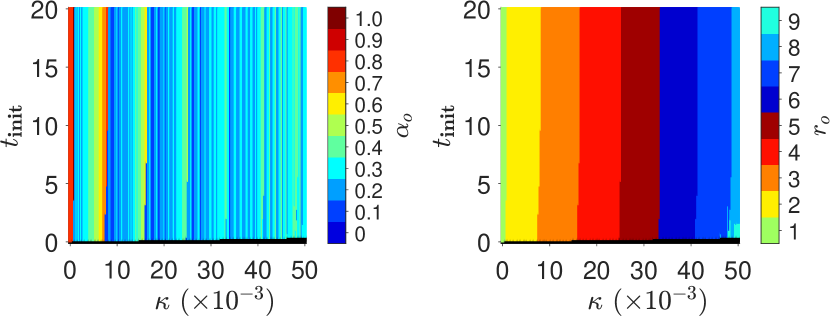
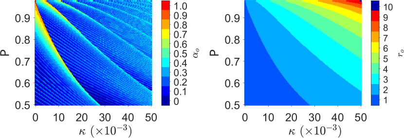
Figure 16: (color online) Optimal hybrid search parameter $\alpha_{o}$ and number of runs $r_{o}$ for multiple-run searching on an $n=7$ hypercube. The optimal search is that which achieves the target success probability $\mathsf{P}$ in the shortest total time $r(t_{\text{init}}+t_{f})$, where $t_{\text{init}}$ and $t_{f}$ are the initialization and run times respectively. Top row: dependence on $t_{\text{init}}$ and decoherence rate $\kappa$ when $\mathsf{P}$ is fixed to $0.95$. Black indicates the region of instantaneous measuring with $t_{f}=0$, where $r=382$. Bottom row: dependence on $\mathsf{P}$ and $\kappa$ when $t_{\text{init}}$ is fixed to 10. LHS plots show $\alpha_{o}$, RHS plots show $r_{o}$. Analytic expression (21) used for AQC schedule. Time and rate units given by Eq. (25).

As $\kappa$ is increased, there is a localized trend for more AQC-like searches to be optimal, however this is punctuated with discontinuous changes to a more QW-like search. The reason for these discontinuous changes can be seen in the right plots of Fig. 16. The boundaries where another run is required correspond exactly to the regions where the optimal value of $\alpha$ suddenly drops. This transition arises when the decoherence rate $\kappa$ and/or target success probability $\mathsf{P}$ have increased such that the best performing strategy with $r$ searches drops below $\mathsf{P}$, and another run is required. In this case the target can be reached by $r+1$ lower quality searches. This drop in the quality required of the single search means a faster, more QW-like search can be used to succeed, and therefore the optimal value of $\alpha$ drops.

Our numerical results for hybrid algorithms in the presence of noise can be understood intuitively by considering how $\mathsf{P}$ scales with a small amount of noise in the AQC and QW edge cases. For noise rate $\kappa$ per unit time, the success probability for a single run reduces as $\mathsf{P}\simeq\exp(-\kappa t_{f})$, where $t_{f}$ is the time taken for one run of the search algorithm. For $\mathsf{P}\sim 1$ we thus require $\kappa t_{f}\ll 1$, i.e., $\kappa\ll 1/t_{f}$. For QW searching on the hypercube, we have $t_{f}^{(\text{QW})}\simeq\frac{\pi}{2}\sqrt{N}$, hence we obtain $\kappa_{\text{QW}}\ll 2/(\pi\sqrt{N})$ for tolerable noise rates. For AQC on the other hand, from Eqn. (24) we have $t_{f}^{(\text{AQC})}\simeq\frac{\pi}{4\epsilon}\sqrt{N}$ for large $N$. For high success probability, since $\mathsf{P}\sim 1-\epsilon$, the adiabatic condition requires $\epsilon\ll 1$ and we obtain $\kappa_{\text{AQC}}\ll 4\epsilon/(\pi\sqrt{N})$. The extra factor of $\epsilon$ implies $\kappa_{\text{AQC}}\ll\kappa_{\text{QW}}$. Hence, QW search will be more robust to disturbance by noise, as we have found numerically for the single run case. For our $n=7$ example, $\kappa_{\text{QW}}\ll 0.056$ and $\kappa_{\text{AQC}}\ll 0.11\epsilon$ = 0.011 for $\mathsf{P}=0.99$, and indeed we see in Fig. 14 that performance drops below $\mathsf{P}=0.5$ for $\kappa_{\text{QW}}\gtrsim 0.025$. However, when multiple runs are included, hybrid strategies with significant adiabatic character can still outperform QW, depending on hardware characteristics determining the initialization and measurement time required per run.

VI Problem misspecification

So far we have studied the dynamics of the hybrid search Hamiltonians, as part of single and multiple run algorithms, and in the presence of noise. In the following section we consider misspecification of the problem, for which the dynamics remain coherent, but some parameters are changed in unknown ways.

VI.1 Motivation

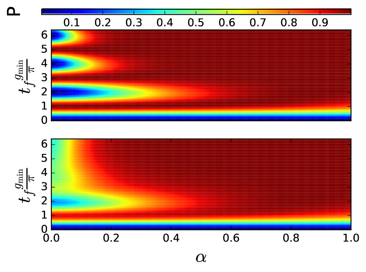
Figure 17: Top: Probability $\mathsf{P}$ of finding the marked state versus runtime and $\alpha$ for the single avoided crossing model, same as Fig. 11. Bottom: as above with a $30\%$ misspecification of the energy $\Delta g_{\text{min}}$.

Studying the effects of problem misspecification is particularly relevant given the critical difficulties which many classical analog computing efforts have faced due to propagation of errors C (2004). Misspecifications can come about in a variety of ways, such as limited precision for setting the controls in the computer, ignorance of what the optimal parameters should be, or noise which is at a much lower frequency than the rate of the relevant quantum dynamics. An important example of the latter is so-called $\frac{1}{f}$ noise in superconducting qubit devices Koch et al. (1983, 2007), such as the quantum annealers constructed by D-Wave Systems Inc. It has been shown, for instance, that such misspecifications can cause AQC to give an incorrect solution on Ising spin systems Young et al. (2013); Albash et al. (2018), and it effectively limits the maximum useful size of such devices. For an example of the effects of problem misspecification on a real experiment, see Chancellor et al. (2016b).

For this work, we will consider simple misspecification models in the large system limit, where the Hamiltonian can be mapped to a single avoided crossing in the form of Eq. (IV.5) or (41). For the purpose of studying problem misspecification, it is most convenient to work with the form in Eq. (41), which we use for the duration of this section. Because the initial and marked states are orthogonal in this limit, considering multiple runs which can be performed with negligible initialization time is not mathematically pathological. Furthermore, physically, we expect initialization and readout time to scale, at worst, polynomially with $n$, while runtime will scale as $\sqrt{N}\propto 2^{\frac{n}{2}}$. Therefore, in the large $N$ limit, it is a natural physical assumption that $t_{f}\gg t_{init}$. We first examine the effect of having the size of the minimum gap be misspecified, so that we do not know when to measure for QW protocols, and then examine the effect of not knowing the position of the avoided crossing, which will cause QW protocols to use the wrong value of $\gamma$ and AQC protocols to slow down at the wrong point.

VI.2 Error in gap size

The effect of misspecifying the size of the minimum gap can be modelled as an uncertainty in the total energy scale $\Delta g_{\text{min}}$, which is equivalent to a misspecification of the total runtime $t_{f}$ through Eq. (41). The effect of uncertainty can be modelled by performing a convolution of the success probability versus runtime with a distribution describing the uncertainty. An example result of such a convolution is depicted in Fig. 17 bottom. Assuming that the misspecification is distributed in a Gaussian manner around the intended runtime, the new success probability for a given anneal time $t_{f}$ and $\alpha$ becomes

$$\mathsf{P}(t_{f},\alpha,\Delta g_{\text{min}})=$$

$$\int_{-\infty}^{\infty}dt_{f}^{\prime}\frac{\mathsf{P}(|t_{f}^{\prime}|,\alpha)}{\Delta g_{\text{min}}\sqrt{2\,\pi}}\exp\left\{-\frac{(t_{f}^{\prime}-t_{f})^{2}}{2(\Delta g_{\text{min}}t_{f})^{2}}\right\},$$ (45)

where $\Delta g_{\text{min}}$ is the (unitless) fractional uncertainty in $g_{\text{min}}$, and the absolute value in the argument of $\mathsf{P}$ within the integral is included to avoid negative time arguments. For reasonable values of $\Delta g_{\text{min}}$, it will be rare for $t_{f}^{\prime}<0$ and the effect of taking the absolute value will be negligible.

Fig. 17 shows how the evolution makes a smooth transition between the characteristically sinusoidal behavior of success probability versus runtime for QW, and the characteristically monotonic behavior of AQC. As the comparison between the perfect and misspecified cases demonstrates, gap misspecification causes a large reduction in the success probability of QW protocols, but has almost no effect on the monotonic AQC search.

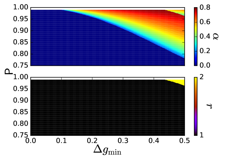
Figure 18: (color online) Top: Optimal value of $\alpha$ versus success probability $\mathsf{P}$ and $\Delta g_{\text{min}}$ from Eq. (45). Bottom: number of repeats $r$ in optimal strategy versus $\mathsf{P}$ and $\Delta g_{\text{min}}$.

Fig. 18 illustrates that, for moderately high success probability and moderate amounts of misspecification of $\Delta g_{\text{min}}$, the best protocol is no longer QW, but lies in between the optimal AQC schedule and QW. For large gap misspecification where a high success probability is required, the best approach is to run an intermediate strategy twice.

The reason that gap size misspecification makes hybrid protocols ($\alpha>0$) outperform QW for a large range of parameter space is because a QW can only succeed with a probability approaching one if $t_{f}\,g_{\text{min}}$ is an odd multiple of $\pi$. The misspecification smears out these peaks and implies that the success probability of a QW will not approach one for any value of $t_{f}$. For protocols with some adiabatic character, however, the maximum success probability will still approach one as $t_{f}$ becomes larger, as the adiabatic theorem holds for any finite gap. In cases where the misspecification overstates the size of the gap the success probability of AQC will actually improve.

VI.3 Error in avoided crossing location

Another type of problem misspecification is incorrectly specifying the position of the avoided crossing. To model this, we consider a modification of the problem Hamiltonian

$$\hat{H}^{(\text{AC})\prime}(t,q)=\hat{H}^{(\text{AC})}(t)+\frac{q}{2}g_{\text{min}}\hat{\sigma}_{z}.$$ (46)

This addition to the problem Hamiltonian provides a shift in the avoided crossing position $f(t)\rightarrow f(t)+q$ in Eq. (41). Effectively introducing this shift causes the schedule to slow down at the wrong point, reducing the success probability. As we did for the case of gap mis-specification, we can model the effect of this error as a convolution of the success probability distribution with $q$ with a Gaussian of width $\Delta q$. We define the success probability with misspecified avoided crossing position as

$$\mathsf{P}(t,\alpha,\Delta q)=\int_{-\infty}^{\infty}dq\frac{\mathsf{P}(t,\alpha,q)}{\Delta q\,\sqrt{2\,\pi}}\,\exp\left(-\frac{q^{2}}{2\,(\Delta q)^{2}}\right),$$ (47)

where $\Delta q$ is the (unitless) fractional uncertainty in $q$, that controls the degree of misspecification. Figure 19 illustrates that, in contrast to gap misspecification, the best strategy is almost always QW. Intermediate strategies only become the superior method briefly, at the edge of the regime where single runs are the best way to reach the desired probability. At higher misspecification, multiple repeated QW become the best strategy.

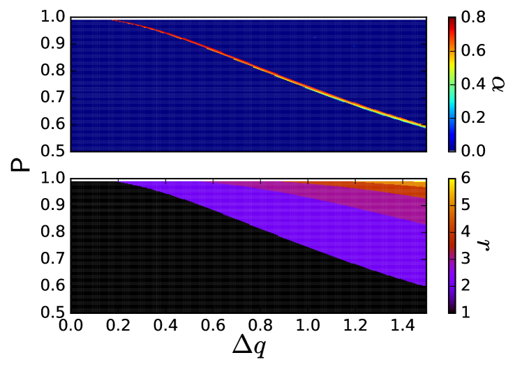
Figure 19: (color online) Top: Optimal value of $\alpha$ versus success probability $\mathsf{P}$ and $\Delta q$ from Eq. (47). Bottom: number of repeats $r$ in optimal strategy versus $\mathsf{P}$ and $\Delta q$.

Misspecification in the avoided crossing position does significant harm to both AQC and QW protocols. The success probability of a QW protocol performed with an incorrectly chosen $\gamma$ does not approach one. Similarly, an AQC protocol with a poorly chosen schedule will require a much longer runtime for the success probability to approach one. The faster runtime of QW then means it beats AQC for multiple runs.

VII Summary and outlook

In this paper we provide a detailed study of the scaling of continuous-time quantum search algorithms on a hypercube graph. Noting that both quantum walk and adiabatic quantum search algorithms can be expressed as two extremes of quantum annealing schedules, we define a family of quantum search algorithms that are hybrids between QW and AQC. By mapping the algorithms to a one qubit single avoided crossing model, we show that the whole family achieves the maximum possible $\sqrt{N}$ quantum speed up. There are a number of subtleties in the scaling behavior on the hypercube that we treat in detail for short search times, complementing the work by Weibe and Babcock Weibe and Babcock (2012) on long timescales.

Our hybrid QW-AQC schedules are an example of the advantages we gain by treating both QW and AQC as part of the same method of continuous-time quantum computing Kendon et al. (2018). We find that hybrid strategies intermediate between QW and AQC provide the best quantum search algorithm under a range of realistic conditions. The techniques we use here can easily be extended to hybrid quantum search on other graphs, and to other quantum walk or adiabatic quantum computing algorithms.

This work focused on the search problem due to its relative simplicity, and the fact that annealing schedules can be derived analytically – which we do for the hypercube graph in appendix A. The core ideas and methods are quite general and can easily be extended to more complex and realistic problems, such a ‘fixed point search’, where multiple states are marked. Fixed point search algorithms have been studied in both the QW Yoder et al. (2014) and AQC Dalzell et al. (2017) regimes, so interpolation to generate hybrid algorithms should be straightforward. The quantum walk search on random graphs solved in Chakraborty et al. (2016) is based on the same kind of single avoided crossing arguments which appear in this work, meaning that these are also natural for hybrid QW-AQC protocols.

Hybrid algorithms such as the ones we present here can be viewed as particular instances of quantum control techniques applied to solving optimization and search problems. Another application of quantum control to quantum algorithms is based on the Pontryagin minimum principle of optimal control: that optimal control protocols for solving these problems will follow a bang-bang scheme, with successive applications of the extreme values of the controls Yang et al. (2017). An algorithm based on such controls, called the Quantum Approximate Optimization Algorithm (QAOA), was first proposed by Farhi, Goldstone, and Gutmann Farhi et al. (2014a, b). This protocol can be implemented either through digital quantum circuits, or by successively applied Hamiltonians. It has been shown that the QAOA can obtain an optimal $\sqrt{N}$ scaling in solving the search problem using a transverse field search unitary Jiang et al. (2017), essentially the problem we consider in this paper.

However, there are two caveats worth noting in terms of the optimality of QAOA type bang-bang protocols. Firstly, when viewed as an application of successive Hamiltonians, these protocols require infinitely fast switching time, which is generally unphysical. Secondly, while the optimal control scheme to find the solution is mathematically always of a bang-bang form, this solution may exhibit Fuller’s phenomenon Borisov (2000); fuller (1960), in which the optimal solution involves switching back and forth between the two extremal Hamiltonians an infinite number of times in a finite time window. While mathematically valid, such a control scheme is clearly not physically realizable. It is an open question what happens to Hamiltonian-based QAOA when finite switching time is added as a constraint. Our result that intermediate protocols between quantum walk and adiabatic protocols are still able to obtain an optimal speed up provide an encouraging sign that QAOA may remain effective with realistic constraints applied.

Recent studies by Muthukrishnan et al. Muthukrishnan et al. (2015, 2016) on a class of permutation symmetric problems related to, but distinct from, search, have found that, deep in the diabatic regime, the problem can be solved by dynamics which are effectively classical through ‘diabatic cascades’. Muthukrishnan et al. focus only on changing the rate of evolution of an AQC algorithm; in contrast, we examine both the shape of the schedule and the rate of evolution. Furthermore, since all of the qubits need to align to interact meaningfully with the energy landscape of the search problem, it is unlikely that a similar classical diabatic cascade regime exists in our study.

As well as problem size, the performance of a quantum search in a realistic setting will depend on many other factors. By performing a fairly general and multi-faceted analysis of such factors, we uncover a landscape where no single protocol dominates. In asymptotically large systems with perfectly specified problems, a straightforward QW approach is best. However, this limit is approached slowly, since the success probability for QW scales only as $n$, i.e., logarithmically in problem size $N$. A rich structure exists for computationally interesting, non-asymptotic sizes. On the other hand, for asymptotically large systems with some degree of problem misspecification, interpolated protocols can outperform the QW approach. A simple open systems analysis reveals another layer of structure that can be exploited in realistic settings. For more discussion on the effects of noise and the competition between the mechanisms, see our related work Morley et al. (2018). In future work we will apply these techniques to algorithms with useful applications which can be run on near-future quantum hardware Callison et al. (2018).

Appendix A Hypercube optimal schedule calculation

Starting from the Hamiltonian for the AQC search on a hypercube, Eq: (14)

$$\hat{H}(s)=(1-s)\sum_{j=1}^{n}\frac{1}{2}(1-\hat{\sigma}^{(j)}_{x})+s(\openone-|m\rangle\!\langle m|),$$

we first apply a gauge transformation (a swap of the $1\leftrightarrow 0$ labels on a subset of the qubits) to map the marked state $|m\rangle$ to the state $|0\rangle$. We then express the Hamiltonian in the symmetric subspace in terms of total spin operators

$$\hat{S}_{a}=\frac{1}{2}\sum_{j=1}^{n}\hat{\sigma}^{(j)}_{a}$$ (48)

for $a\in\{x,y,z\}$, which have eigenstates $|\frac{n}{2}-r\rangle_{a}$ for $r\in\{0,\dots,n\}$. In this representation, the marked state is $|\frac{n}{2}\rangle_{z}$, and the AQC search Hamiltonian becomes

$$\hat{H}(s)=(1-s)(\tfrac{n}{2}-\hat{S}_{x})+s(\openone-|\tfrac{n}{2}\rangle_{z}\langle\tfrac{n}{2}|).$$ (49)

Following Farhi et al Farhi et al. (2000) to analyze the eigensystem, we obtain the eigenvalue equation

$$\frac{1-s}{s}=\frac{1}{N}\sum_{r=0}^{n}\left(\begin{array}[]{c}n\\ r\\ \end{array}\right)\frac{1}{r-\lambda}$$ (50)

for the energy eigenvalues $E_{k}=s+(1-s)\lambda_{k}$. Farhi et al Farhi et al. (2000) solve this at the minimum gap, which occurs at $s=s_{m}$ for

$$\frac{1-s_{m}}{s_{m}}=\frac{1}{N}\sum_{r=1}^{n}\left(\begin{array}[]{c}n\\ r\\ \end{array}\right)\frac{1}{r}\equiv R_{1},$$ (51)

and show that $\lambda^{(\text{gmin})}_{1,0}\simeq\pm n/(2\sqrt{N})$ for the two lowest eigenvalues corresponding the the ground state $E_{0}$ and first excited state $E_{1}$.

To obtain the optimal schedule following the method in Roland and Cerf Roland and Cerf (2002), we need an expression for the gap as a function of $s(t)$, not just at the minimum gap. We expand the eigenvalue equation (50) for $\lambda\ll 1$

$$\frac{1-s}{s}=\frac{-1}{N\lambda}+\frac{1}{N}\sum_{r=1}^{n}\left(\begin{array}[]{c}n\\ r\\ \end{array}\right)\frac{1}{r}(1+\lambda/r)+O(\lambda^{2}).$$ (52)

Using $R_{1}$ and $R_{2}$ from Eqs. (10), (51) and (23) we obtain

$$\frac{1-s}{s}=\frac{-1}{N\lambda}+R_{1}+\lambda R_{2}.$$ (53)

This quadratic equation in $\lambda$ has roots

$$\lambda= \frac{1}{2R_{2}}\left\{\frac{1-s}{s}-R_{1}\right\}$$

$$\pm\frac{1}{2}\left\{\frac{1}{R_{2}^{2}}\left(\frac{1-s}{s}-R_{1}\right)^{2}+\frac{4}{NR_{2}}\right\}^{\frac{1}{2}}$$ (54)

and gives for the gap $g(s)=(1-s)(\lambda_{1}-\lambda_{0})$

$$g(s)=(1-s)\left\{\frac{1}{R_{2}^{2}}\left(\frac{1-s}{s}-R_{1}\right)^{2}+\frac{4}{NR_{2}}\right\}^{\frac{1}{2}}.$$ (55)

To optimize the schedule, we need to solve Eq. (16)

$$\left\lvert\frac{ds}{dt}\right\rvert\leq\epsilon\frac{g^{2}(s)}{\left\lvert\left\langle\frac{d\hat{H}}{ds}\right\rangle_{0,1}\right\rvert}$$

using the expression for $g(s)$ in Eq. (55). To obtain a suitable approximate value for $\langle\frac{d\hat{H}}{ds}\rangle_{0,1}$, we first calculate $\frac{d\hat{H}}{ds}$ in the symmetric subspace representation of Eq. (49),

$$\frac{d\hat{H}}{ds}=-(\tfrac{n}{2}-\hat{S}_{x})+(\openone-|\tfrac{n}{2}\rangle_{z}\langle\tfrac{n}{2}|).$$ (56)

It is sufficient to use the maximum value of $\langle\frac{d\hat{H}}{ds}\rangle_{0,1}$, which occurs at $s_{m}$, where the eigenstates $|E_{1,0}\rangle\simeq(|\frac{n}{2}\rangle_{x}\pm|\frac{n}{2}\rangle_{z})/\sqrt{2}$, giving $\langle\frac{d\hat{H}}{ds}\rangle_{0,1}^{(\text{max})}\leq\frac{n}{4}$. We then have the following equation to solve for $s(t)$

$$\frac{ds}{dt}=\frac{4\epsilon}{nR_{2}^{2}}(1-s)^{2}\left\{\left(\frac{1-s}{s}-R_{1}\right)^{2}+\frac{4R_{2}}{N}\right\}$$ (57)

This can be integrated to obtain

$$\frac{4\epsilon t}{nR_{2}^{2}}+c =\frac{R_{1}^{2}-4R_{2}/N}{2\sqrt{R_{2}/N}(R_{1}^{2}+4R_{2}/N)^{2}}$$

$$\arctan\left\{\frac{((1+R_{1})^{2}+4R_{2}/N)s-(1+R_{1})}{2\sqrt{R_{2}/N}}\right\}$$

$$+\frac{1}{(1-s)(R_{1}^{2}+4R_{2}/N)}$$

$$+\frac{R_{1}}{(R_{1}^{2}+4R_{2}/N)^{2}}\ln\left\{\frac{(1-s-R_{1}s)^{2}+\frac{4R_{2}}{N}s^{2}}{(1-s)^{2}}\right\}$$ (58)

where $c$ is the constant of integration. To obtain the constant, set $s=t=0$, giving

$$c^{\prime}=\arctan\left\{\frac{(1+R_{1})\sqrt{N}}{2\sqrt{R_{2}}}\right\}+\frac{R_{1}^{2}+4R_{2}/N}{R_{1}^{2}-4R_{2}/N}\frac{2\sqrt{R_{2}}}{\sqrt{N}}$$ (59)

where the factors in front of the arctan term have been rearranged to give a more convenient form for the constant. One can then in principle solve for $s(t)$. However, the terms on the r.h.s., apart from the arctan, are potentially problematic as $s\rightarrow 1$. Given that we started with the approximation $\lambda\ll 1$, which occurs at the position of the minimum gap, we can’t necessarily expect that the solution will be valid for $s\rightarrow 1$. We first note that taking only the arctan term on the r.h.s. gives a schedule that is valid for all $0\leq s\leq 1$, and it provides a runtime proportional to $\sqrt{N}$. If we don’t discard these extra terms, we can show that they can be neglected, provided we stop the anneal very slightly before $s=1$, but still well past the minimum gap.

To solve for $s(t)$ retaining the full expression, invert the arctan to give

$$s(t)= \frac{2\sqrt{R_{2}}}{\sqrt{N}\{(1+R_{1})^{2}+4R_{2}/N\}}\times$$

$$\tan\left\{\frac{8\epsilon t\sqrt{R_{2}}}{nR_{2}^{2}\sqrt{N}}\frac{R_{1}^{2}+4R_{2}/N}{R_{1}^{2}-4R_{2}/N}-c^{\prime\prime}\right\}$$

$$+\frac{1+R_{1}}{(1+R_{1})^{2}+4R_{2}/N},$$ (60)

where $c^{\prime\prime}$ now contains the awkward extra terms,

$$c^{\prime\prime}= c^{\prime}-\frac{1}{(1-s)}\frac{R_{1}^{2}+4R_{2}/N}{R_{1}^{2}-4R_{2}/N}\frac{2\sqrt{R_{2}}}{\sqrt{N}}$$

$$-\frac{R_{1}}{R_{1}^{2}-4R_{2}/N}\frac{2\sqrt{R_{2}}}{\sqrt{N}}\ln\left\{\frac{(1-s-R_{1}s)^{2}+\frac{4R_{2}}{N}s^{2}}{(1-s)^{2}}\right\}$$

$$= \arctan\left\{\frac{(1+R_{1})\sqrt{N}}{2\sqrt{R_{2}}}\right\}$$

$$+\frac{s}{(1-s)}\frac{R_{1}^{2}+4R_{2}/N}{R_{1}^{2}-4R_{2}/N}\frac{2\sqrt{R_{2}}}{\sqrt{N}}$$

$$-\frac{R_{1}}{R_{1}^{2}-4R_{2}/N}\frac{2\sqrt{R_{2}}}{\sqrt{N}}\ln\left\{\frac{(1-s-R_{1}s)^{2}+\frac{4R_{2}}{N}s^{2}}{(1-s)^{2}}\right\}.$$ (61)

The arctan argument is large, so the arctan is close to $\pi/2$. We note that the extra terms are small for most values of $s$, and only become large as $s\rightarrow 1$. To check when these terms become $O(1)$, for the first extra term we solve

$$\frac{s}{(1-s)}\frac{R_{1}^{2}+4R_{2}/N}{R_{1}^{2}-4R_{2}/N}\frac{2\sqrt{R_{2}}}{\sqrt{N}}\simeq 1$$ (62)

to obtain

$$s\simeq\frac{1}{1+2\sqrt{R_{2}/N}}\simeq\frac{1}{1+4/(n\sqrt{N})}.$$ (63)

This is well past the minimum gap, which occurs at $s=1/(1+R_{1})\simeq 1/(1+2/n)$. Applying the same procedure to the second extra term gives to leading order

$$s\simeq 1-e^{-\sqrt{N}/4},$$ (64)

which is even closer to $s=1$ and further from the minimum gap. Since the transition probabilities are only significant close to the minimum gap, and hence all the important slowing down of the schedule occurs around the gap, what happens this close to $s=1$ has essentially no effect on the success or runtime of the algorithm.

Dropping the extra terms from the solution provides an expression for $s(t)$

$$s(t)=\frac{2\sqrt{R_{2}}}{\sqrt{N}(1+R_{1})^{2}}\tan\left\{\frac{8\epsilon\sqrt{R_{2}}R_{1}^{2}t}{n\sqrt{N}R_{2}^{2}}-c^{\prime\prime\prime}\right\}+\frac{1}{1+R_{1}}$$ (65)

where we have also dropped terms $O(1/N)$, and

$$c^{\prime\prime\prime}=\arctan\left\{\frac{(1+R_{1})\sqrt{N}}{2\sqrt{R_{2}}}\right\}.$$ (66)

Strictly speaking, this is valid for $s\lesssim\frac{1}{1+4/(n\sqrt{N})}$, although in fact it is well-behaved right up to and including $s=1$. From this we can obtain the runtime

$$\epsilon\,t_{f}\simeq\frac{\pi\sqrt{N}}{4},$$ (67)

where the two arctan terms have each been approximated by $\pi/2$, since their arguments are large, $O(\sqrt{N})$.

Appendix B Numerical methods

Our numerical calculations were carried out using the Python programming language (both Python 2.7 and Python 3.5), making considerable use of the NumPy, SciPy and Matplotlib packages pyt (2016); num (2016); sci (2016); mat (2016). High performance computing resources were not used in this study, although some of the simulations took several days to run on standard desktop workstations. Most of the simulations consisted of solving the time evolution of the quantum search algorithm by numerically integrating the Schrödinger equation using the appropriate Hamiltonian. This was done by diagonalising the Hamiltonian and exponentiating it in the diagonal basis, before applying it to the wave function. This process was iterated for time dependent Hamiltonians, rotating from one instantaneous diagonal basis to the next at small time intervals. For the decoherence studies in Sec. V.3, the same process was applied to the density matrix, with dephasing operators also applied along with the unitary time evolution.

For larger simulations, we can take advantage of the symmetry in the hypercube to map the dynamics to a search on the line with appropriately weighted edges, as given by Eq. (49) in appendix A. Provided the initial state is also invariant with respect this symmetry, the evolution will be restricted to this symmetric subspace. This allows us to perform simulations for much larger numbers of qubits $n\lesssim 100$, and hence extract reliable information about the scaling with $n$ from numerics alone. This provides important checks of the validity of the two-level approximations made to facilitate the analytical calculations.

Optimal AQC schedules $s^{(n)}(\tau)$ were calculated numerically as solutions of Eq. (20), both to check the analytical solutions for the hypercube, and because we can solve numerically with less approximations than are required to obtain analytical expressions. Specifically, we calculate the gap $g(s)$ directly from the Hamiltonian eigensystem, rather than expanding about $g_{\text{min}}$ as was done in appendix A. However, we do make the same approximation in the analytics and numerics by using the maximum value of $\frac{n}{4}$ for $\langle\frac{d\hat{H}}{ds}\rangle_{0,1}$ obtained in appendix A. For the hypercube, the matrix which describes these systems is $(n+1)\times(n+1)$, even after taking advantage of symmetry by mapping to a line. A Hermitian $2\times 2$ matrix can always be diagonalized analytically by finding the roots of the characteristic polynomial, as was done in Roland and Cerf (2002). For larger matrices this is no longer feasible, nor generally possible if the matrix is bigger than $4\times 4$. Fortunately, the gap $g(s)$ can easily be calculated numerically using the iterative eigensolving modules in Numpy num (2016), and we are thence able to iteratively solve $\left|\frac{ds}{dt}\right|=\epsilon 4g^{2}(s)/n$. We first define a normalized function

$$F(s)=\int_{0}^{s}ds^{\prime}\frac{1}{\epsilon g^{2}(s^{\prime})}\times\left[\int_{0}^{1}ds^{\prime}\frac{1}{\epsilon g^{2}(s^{\prime})}\right]^{-1},$$ (68)

where $s$ is a function of the reduced time $\tau$. To obtain $s(\tau)$, we need to invert this function, $s(\tau)=F^{-1}(\tau)$. The following method accomplishes this.

Deliberately using a programming-like notation, we define $\tau\text{{List}}$ to be a linearly spaced list of points between $\tau=0$ and $\tau=1$, and $s\text{{List}}$ to be a list of the corresponding values of $s(\tau)$, obtained by applying $F^{-1}(\tau)$ to each element of $\tau\text{{List}}$. Defining $j(s)$ equal to the number of elements in $s\text{{List}}$ which are strictly less than $s$, we approximate $F(s)$ numerically by $\tilde{F}(s)$, where we replace the integral by a finite sum plus linear interpolation. Writing $\tilde{s_{j}}=\frac{1}{2}(s\text{{List}}(j(s))+s\text{{List}}(j(s)+1))$

$$\tilde{F}(s) =\sum_{j^{\prime}=1}^{j(s)}\frac{s\text{{List}}(j^{\prime}+1)-s\text{{List}}(j^{\prime})}{\mathcal{N}\,g^{2}\left(\tilde{s_{j^{\prime}}}\right)}$$

$$+\frac{s-s\text{{List}}(j(s))}{\mathcal{N}\,g^{2}\left(\tilde{s_{j}}\right)},$$ (69)

where $\mathcal{N}$ is a normalization factor which is included to ensure that $\hat{F}(s=1)=1$. It is straightforward to numerically invert $\hat{F}(s)$. This can be accomplished by first finding $j_{\max}(s)$, the largest value of $j(s)$ for which $\hat{F}(s)<\tau$, and then solving

$$\hat{F}(s)|_{j(s)=j_{\max}(s)}=\tau$$ (70)

for $s$. Based on this numerical function inversion, we define an iterative method of converging on the solution for $s^{(n)}(\tau)$,

1. set a linearly spaced $s\text{{List}}\in[0,1]$ and $\tau\text{{List}}\in[0,1]$ each with the same number of elements

2. using the values of $s$ in $s\text{{List}}$, apply $\hat{F}^{-1}(\tau)$ to each corresponding element in $\tau\text{{List}}$ to generate a new $s\text{{List}}$

3. repeat step 2. with the new $s\text{{List}}$ as input, until it has converged

The advantage of this iterative method is that, at each iteration, more points in $s\text{{List}}$ will concentrate in areas where $1/g^{2}$ is larger, for instance near the dominant avoided crossing. By using the previously calculated $s\text{{List}}$ as a mesh in the current iteration, the protocol can continuously improve the quality of the numerical inverse with a fixed number of points in $s\text{{List}}$.

References

- Brooke et al. (1999) J. Brooke, D. Bitko, T. F. Rosenbaum, and G. Aeppli, “Quantum annealing of a disordered magnet,” Science 284, 779–781 (1999), http://science.sciencemag.org/content/284/5415/779.full.pdf .
- Johnson et al. (2011) M. W. Johnson, M. H. S. Amin, S. Gildert, T. Lanting, F. Hamze, N. Dickson, R. Harris, A. J. Berkley, J. Johansson, P. Bunyk, E. M. Chapple, C. Enderud, J. P. Hilton, K. Karimi, E. Ladizinsky, N. Ladizinsky, T. Oh, I. Perminov, C. Rich, M. C. Thom, E. Tolkacheva, C. J. S. Truncik, S. Uchaikin, J. Wang, and B. Wilsonand G. Rose, “Quantum annealing with manufactured spins,” Nature 473, 194–198 (2011).
- Denchev et al. (2016) Vasil S. Denchev, Sergio Boixo, Sergei V. Isakov, Nan Ding, Ryan Babbush, Vadim Smelyanskiy, John Martinis, and Hartmut Neven, “What is the computational value of finite-range tunneling?” Phys. Rev. X 6, 031015 (2016).
- Lanting et al. (2014) T. Lanting, A. J. Przybysz, A. Yu. Smirnov, F. M. Spedalieri, M. H. Amin, A. J. Berkley, R. Harris, F. Altomare, S. Boixo, P. Bunyk, N. Dickson, C. Enderud, J. P. Hilton, E. Hoskinson, M. W. Johnson, E. Ladizinsky, N. Ladizinsky, R. Neufeld, T. Oh, I. Perminov, C. Rich, M. C. Thom, E. Tolkacheva, S. Uchaikin, A. B. Wilson, and G. Rose, “Entanglement in a quantum annealing processor,” Phys. Rev. X 4, 021041 (2014).
- Boixo et al. (2016) Sergio Boixo, Vadim N. Smelyanskiy, Alireza Shabani, Sergei V. Isakov, Mark Dykman, Vasil S. Denchev, Mohammad H. Amin, Anatoly Yu Smirnov, Masoud Mohseni, and Hartmut Neven, “Computational multiqubit tunnelling in programmable quantum annealers,” Nature Communications 7 (2016), doi:10.1038/ncomms10327.
- Georgescu et al. (2014) I. M. Georgescu, S. Ashhab, and Franco Nori, “Quantum simulation,” Rev. Mod. Phys. 86, 153–185 (2014).
- Nguyen et al. (2018) T. L. Nguyen, J. M. Raimond, C. Sayrin, R. Cortiñas, T. Cantat-Moltrecht, F. Assemat, I. Dotsenko, S. Gleyzes, S. Haroche, G. Roux, Th. Jolicoeur, and M. Brune, “Towards quantum simulation with circular rydberg atoms,” Phys. Rev. X 8, 011032 (2018).
- Kendon et al. (2018) V.M. Kendon, N. Chancellor, S. Bose, and A. Daley, “Developing continuous-time quantum computing,” (2018), in preparation.
- Marzec (2016) Michael Marzec, “Portfolio optimization: Applications in quantum computing,” in Handbook of High-Frequency Trading and Modeling in Finance (John Wiley & Sons, Inc., 2016) pp. 73–106.
- Russo (2014) G. E.Coxson C. R. Hill J. C. Russo, “Adiabatic quantum computing for finding low-peak-sidelobe codes,” (2014), presented at the 2014 IEEE High Performance Extreme Computing conference.
- Melko (2016) M. H. Amin E. Andriyash J. Rolfe B. Kulchytskyy R. Melko, “Quantum Boltzmann machine,” (2016), arXiv:quant-ph:1601.02036 .
- Benedetti et al. (2016a) M. Benedetti, J. Realpe-Gómez, R. Biswas, and A. Perdomo-Ortiz, “Estimation of effective temperatures in quantum annealers for sampling applications: A case study with possible applications in deep learning,” Phys. Rev. A 94, 022308 (2016a).
- Benedetti et al. (2016b) M. Benedetti, J. Realpe-Gómez, R. Biswas, and A. Perdomo-Ortiz, “Quantum-assisted learning of graphical models with arbitrary pairwise connectivity,” (2016b), arXiv:1609.02542 .
- Chancellor et al. (2016a) N. Chancellor, S. Zohren, P. Warburton, S. Benjamin, and S. Roberts, “A direct mapping of Max k-SAT and high order parity checks to a chimera graph,” Scientific Reports 6 (2016a), 10.1038/srep37107, arXiv:1604.00651 .
- Chancellor et al. (2016b) N. Chancellor, S. Szoke, W. Vinci, G. Aeppli, and P. A. Warburton, “Maximum–entropy inference with a programmable annealer,” Scientific Reports 6 (2016b), doi:10.1038/srep22318.
- Li et al. (2017) Zhaokai Li, Nikesh S. Dattani, Xi Chen, Xiaomei Liu, Hengyan Wang, Richard Tanburn, Hongwei Chen, Xinhua Peng, and Jiangfeng Du, “High-fidelity adiabatic quantum computation using the intrinsic hamiltonian of a spin system: Application to the experimental factorization of 291311,” (2017), arXiv:1706.08061 .
- Bian et al. (2013) Zhengbing Bian, Fabian Chudak, William G. Macready, Lane Clark, and Frank Gaitan, “Experimental determination of ramsey numbers,” Phys. Rev. Lett. 111, 130505 (2013).
- Perdomo-Ortiz et al. (2012) Alejandro Perdomo-Ortiz, Neil Dickson, Marshall Drew-Brook, Geordie Rose, and Alan Aspuru-Guzik, “Finding low-energy conformations of lattice protein models by quantum annealing,” Scientific Reports 2 (2012).
- Grover (1997) L. K. Grover, “Quantum mechanics helps in searching for a needle in a haystack,” Phys. Rev. Lett. 79, 325 (1997), arXiv:quant-ph/9706033 .
- Bennett et al. (1997) Charles H. Bennett, Ethan Bernstein, Gilles Brassard, and Umesh Vazirani, “Strengths and weaknesses of quantum computing,” SIAM J. Comput. 26, 151–152 (1997).
- Shenvi et al. (2003) Neil Shenvi, Julia Kempe, and K Birgitta Whaley, “A quantum random walk search algorithm,” Phys. Rev. A 67, 052307 (2003), arXiv:quant-ph/0210064 .
- Roland and Cerf (2002) Jérémie Roland and Nicolas J. Cerf, “Quantum search by local adiabatic evolution,” Phys. Rev. A 65, 042308 (2002).
- Lovett et al. (2011) Neil B. Lovett, Matthew Everitt, Robert M. Heath, and Viv Kendon, “The quantum walk search algorithm: Factors affecting efficiency,” (2011), to appear in Math. Struct. Comp. Sci., 1110.4366v1[quant-ph] .
- Coulamy et al. (2017) Ivan B. Coulamy, Andreia Saguia, and Marcelo S. Sarandy, “Dynamics of the quantum search and quench-induced first-order phase transitions,” Phys. Rev. E 95, 022127 (2017).
- Tulsi (2015) Avatar Tulsi, “Postprocessing can speed up general quantum search algorithms,” Phys. Rev. A 92, 022353 (2015).
- Ambainis et al. (2011) Andris Ambainis, Arturs Backurs, Nikolajs Nahimovs, Raitis Ozols, and Alexander Rivosh, “Search by quantum walks on two-dimensional grid without amplitude amplification,” (2011), arXiv:1112.3337 .
- Magniez et al. (2011) Frédéric Magniez, Ashwin Nayak, Jérémie Roland, and Miklos Santha, “Search via quantum walk,” SIAM Journal on Computing 40, 142–164 (2011), quant-ph/0608026v4 .
- Wong and Meyer (2016) Thomas G. Wong and David A. Meyer, “Irreconcilable difference between quantum walks and adiabatic quantum computing,” Phys. Rev. A 93, 062313 (2016).
- Chancellor (2016) Nicholas Chancellor, “Max-k-SAT, multi-body frustration, & multi-body sampling on a two local Ising system,” AQC 2016 https://www.youtube.com/watch?v=aC-6hg_h3EA (2016).
- Chancellor et al. (2018) Nicholas Chancellor, A. Ben Dodds, and Viv Kendon, “Practical designs for permutation symmetric problem Hamiltonians on hypercubes,” (2018), in preparation.
- Childs and Goldstone (2004) Andrew Childs and Jeffrey Goldstone, “Spatial search by quantum walk,” Phys. Rev. A 70, 022314 (2004), quant-ph/0306054 .
- Chakraborty et al. (2016) S. Chakraborty, L. Novo, A. Ambainis, and Y. Omar, “Spatial search by quantum walk is optimal for almost all graphs,” Phys. Rev. Lett. 116 (2016), 10.1103/PhysRevLett.116.100501.
- Moore and Russell (2002) Christopher Moore and Alexander Russell, “Quantum walks on the hypercube,” in Proc. 6th Intl. Workshop on Randomization and Approximation Techniques in Computer Science (RANDOM ’02), edited by J. D. P. Rolim and S. Vadhan (Springer, 2002) pp. 164–178, quant-ph/0104137 .
- Hein and Tanner (2009) Birgit Hein and Gregor Tanner, “Quantum search algorithms on the hypercube,” J. Phys. A: Math. Theor. 42, 085303 (2009).
- Farhi et al. (2000) E. Farhi, J. Goldstone, S. Gutmann, and M. Sipser, “Quantum computation by adiabatic evolution,” (2000), quant-ph/0001106 .
- Childs et al. (2002) A. M. Childs, E. Deotto, E. Farhi, J. Goldstone, S. Gutmann, and A. J. Landahl, “Quantum search by measurement,” Phys. Rev. A 66, 032314 (2002), quant-ph/0204013 .
- Born and Fock (1928) M. Born and V. Fock, “Beweis des adiabatensatzes,” Z. Phys. 51(3-4), 165–180 (1928).
- Albash and Lidar (2018) Tameem Albash and Daniel A. Lidar, “Adiabatic quantum computing,” Rev. Mod. Phys. 90 (2018), 10.1103/RevModPhys.90.015002.
- Lanting (2017) Trevor Lanting, “The D-Wave 2000Q Processor,” (2017), presented at AQC 2017.
- Lidar et al. (2009) Daniel A. Lidar, Ali T. Rezakhani, and Alioscia Hamma, “Adiabatic approximation with exponential accuracy for many-body systems and quantum computation,” Journal of Mathematical Physics 50, 102106 (2009).
- Rezakhani et al. (2009) A. T. Rezakhani, W.-J. Kuo, A. Hamma, D. A. Lidar, and P. Zanardi, “Quantum adiabatic brachistochrone,” Phys. Rev. Lett. 103, 080502 (2009).
- Rezakhani et al. (2010) A. T. Rezakhani, A. K. Pimachev, and D. A. Lidar, “Accuracy vs run time in adiabatic quantum search,” Phys. Rev. A 82, 052305 (2010).
- Weibe and Babcock (2012) Nathan Weibe and Nathan S Babcock, “Improved error-scaling for adiabatic quantum evolutions,” New Journal of Physics 14 (2012), 10.1088/1367-2630/14/1/013024.
- Kieferová and Wiebe (2014) Mária Kieferová and Nathan Wiebe, “On the power of coherently controlled quantum adiabatic evolutions,” New Journal of Physics 16, 123034 (2014).
- Morley et al. (2018) J. G. Morley, N. Chancellor, V. M. Kendon, and S. Bose, “Quench vs adiabacity: balancing competing mechanisms for quantum search on noisy machines,” (2018), co-submitted.
- de Vega et al. (2010) Ines de Vega, Mari Carmen Bañuls, and A. Pérez, “Effects of dissipation in an adiabatic quantum search algorithm,” New J. Phys. 12, 123010 (2010).
- Wild et al. (2016) Dominik S. Wild, Sarang Gopalakrishnan, Michael Knap, Norman Y. Yao, and Mikhail D. Lukin, “Adiabatic quantum search in open systems,” Phys. Rev. Lett. 117, 150501 (2016).
- Alagic and Russell (2005) Gorjan Alagic and Alexander Russell, “Decoherence in quantum walks on the hypercube,” Phys. Rev. A 72, 062304 (2005).
- Richter (2007) Peter C. Richter, “Quantum speedup of classical mixing processes,” Phys. Rev. A 76, 042306 (2007).
- Kendon and Maloyer (2008) Viv Kendon and Olivier Maloyer, “Optimal computation with non-unitary quantum walks,” Theoretical Computer Science 394, 187 – 196 (2008).
- Misra and Sudarshan (1977) B. Misra and E. C. G. Sudarshan, “The Zeno’s paradox in quantum theory,” Journal of Mathematical Physics 18, 756–763 (1977), arXiv:1011.1669v3 .
- C (2004) Bissell C C, “A great disappearing act: the electronic analogue computer,” IEEE Conference on the History of Electronics (Bletchley, UK,) (2004), pages 28–30, available at http://oro.open.ac.uk/id/eprint/5795.
- Koch et al. (1983) Roger H. Koch, John Clarke, W. M. Goubau, J. M. Martinis, C. M. Pegrum, and D. J. van Harlingen, “Flicker (1/f) noise in tunnel junction dc squids,” Journal of Low Temperature Physics 51, 207–224 (1983).
- Koch et al. (2007) Roger H. Koch, David P. DiVincenzo, and John Clarke, “Model for flux noise in squids and qubits,” Phys. Rev. Lett. 98, 267003 (2007).
- Young et al. (2013) Kevin C. Young, Robin Blume-Kohout, and Daniel A. Lidar, “Adiabatic quantum optimization with the wrong Hamiltonian,” Phys. Rev. A 88 (2013), 10.1103/PhysRevA.88.062314.
- Albash et al. (2018) T. Albash, V. Martin-Mayor, and Itay Hen, “Analog errors in ising machines,” (2018), arXiv:1806.03744 .
- Yoder et al. (2014) Theodore J. Yoder, Guang Hao Low, and Isaac L. Chuang, “Fixed-point quantum search with an optimal number of queries,” Phys. Rev. Lett. 113, 210501 (2014).
- Dalzell et al. (2017) Alexander M. Dalzell, Theodore J. Yoder, and Isaac L. Chuang, “Fixed-point adiabatic quantum search,” Phys. Rev. A 95, 012311 (2017).
- Yang et al. (2017) Zhi-Cheng Yang, Armin Rahmani, Alireza Shabani, Hartmut Neven, and Claudio Chamon, “Optimizing variational quantum algorithms using Pontryagin’s minimum principle,” Phys. Rev. X 7, 021027 (2017).
- Farhi et al. (2014a) Edward Farhi, Jeffrey Goldstone, and Sam Gutmann, “A quantum approximate optimization algorithm,” (2014a), arXiv:1411.4028 .
- Farhi et al. (2014b) Edward Farhi, Jeffrey Goldstone, and Sam Gutmann, “A quantum approximate optimization algorithm applied to a bounded occurrence constraint problem,” (2014b), arXiv:1412.6062 .
- Jiang et al. (2017) Zhang Jiang, Eleanor G. Rieffel, and Zhihui Wang, “Near-optimal quantum circuit for Grover’s unstructured search using a transverse field,” Phys. Rev. A 95, 062317 (2017).
- Borisov (2000) V. F. Borisov, “Fuller’s phenomenon: Review,” Journal of Mathematical Sciences, 100, 2311–2354 (2000).
- fuller (1960) A. T. fuller, “Relay control systems optimized for various performance criteria,” in Proc. First World Congress IFAC (1960) pp. 510–519.
- Muthukrishnan et al. (2015) Siddharth Muthukrishnan, Tameem Albash, and Daniel A Lidar, “When diabatic trumps adiabatic in quantum optimization,” (2015), arXiv:1505.01249 .
- Muthukrishnan et al. (2016) Siddharth Muthukrishnan, Tameem Albash, and Daniel A. Lidar, “Tunneling and speedup in quantum optimization for permutation-symmetric problems,” Phys. Rev. X 6, 031010 (2016).
- Callison et al. (2018) Adam Callison, Christian Rennison-Jones, Nicholas Chancellor, and Viv Kendon, “Solving spin-glasses with quantum walks,” (2018), in preparation.
- pyt (2016) “Python 2.7 & Python 3.5,” (2016), https://www.python.org/, accessed August 10th, 2016.
- num (2016) “Numpy 1.11.1,” (2016), http://www.numpy.org/, accessed August 10th, 2016.
- sci (2016) “Scipy 0.17.1,” (2016), https://www.scipy.org/, accessed August 10th, 2016.
- mat (2016) “Matplotlib 1.5.1,” (2016), http://matplotlib.org/, accessed August 10th, 2016.