Sharper and Simpler Nonlinear Interpolants
for Program Verification

Abstract

Interpolation of jointly infeasible predicates plays important roles in various program verification techniques such as invariant synthesis and CEGAR. Intrigued by the recent result by Dai et al. that combines real algebraic geometry and SDP optimization in synthesis of polynomial interpolants, the current paper contributes its enhancement that yields sharper and simpler interpolants. The enhancement is made possible by: theoretical observations in real algebraic geometry; and our continued fraction-based algorithm that rounds off (potentially erroneous) numerical solutions of SDP solvers. Experiment results support our tool’s effectiveness; we also demonstrate the benefit of sharp and simple interpolants in program verification examples. rogram verification · interpolation · nonlinear interpolant · polynomial · real algebraic geometry · SDP optimization · numerical optimization

1 Introduction

Interpolation for Program Verification Interpolation in logic is a classic problem. Given formulas $\varphi$ and $\psi$ that are jointly unsatisfiable (meaning $\models\varphi\land\psi\Rightarrow\bot$), one asks for a “simple” formula $\xi$ such that $\models\varphi\Rightarrow\xi$ and $\models\xi\land\psi\Rightarrow\bot$. The simplicity requirement on $\xi$ can be a formal one (like the common variable condition, see Def. 2.6) but it can also be informal, like “$\xi$ is desirably much simpler than $\varphi$ and $\psi$ (that are gigantic).” Anyway the intention is that $\xi$ should be a simple witness for the joint unsatisfiability of $\varphi$ and $\psi$, that is, an “essential reason” why $\varphi$ and $\psi$ cannot coexist.

This classic problem of interpolation has found various applications in static analysis and program verification [21, 11, 15, 13, 23, 22]. This is particularly the case with techniques based on automated reasoning, where one relies on symbolic predicate abstraction in order to deal with infinite-state systems like (behaviors of) programs. It is crucial for the success of such techniques that we discover “good” predicates that capture the essence of the systems’ properties. Interpolants—as simple witnesses of incompatibility—have proved to be potent candidates for these “good” predicates.

Interpolation via Optimization and Real Algebraic Geometry A lot of research efforts have been made towards efficient interpolation algorithms. One of the earliest is [5]: it relies on Farkas’ lemma for synthesizing linear interpolants (i.e. interpolants expressed by linear inequalities). This work and subsequent ones have signified the roles of optimization problems and their algorithms in efficient synthesis of interpolants.

In this line of research we find the recent contribution by Dai et al. [8] remarkable, from both theoretical and implementation viewpoints. Towards synthesis of nonlinear interpolants (that are expressed by polynomial inequalities), their framework in [8] works as follows.

• On the theory side it relies on Stengle’s Positivstellensatz—a fundamental result in real algebraic geometry [33, 3]—and relaxes the interpolation problem to the problem of finding a suitable “disjointness certificate.” The latter consists of a few polynomials subject to certain conditions.

• On the implementation side it relies on state-of-the-art SDP solvers to efficiently solve the SDP problem that results from the above relaxation.

In [8] it is reported that the above framework successfully synthesizes nontrivial nonlinear interpolants, where some examples are taken from program verification scenarios.

Contribution The current work contributes an enhancement of the framework from [8]. Our specific concerns are in sharpness and simplicity of interpolants.

Example 1.1 (sharp interpolant)

Let $\mathcal{T}\coloneqq(y>x\land x>-y)$ and $\mathcal{T}^{\prime}\coloneqq(y\leq-x^{2})$. These designate the blue and red areas in the figure, respectively. We would like an interpolant $\mathcal{S}$ so that $\mathcal{T}$ implies $\mathcal{S}$ and $\mathcal{S}$ is disjoint from $\mathcal{T}^{\prime}$. Note however that such an interpolant $\mathcal{S}$ must be “sharp.” The areas of $\mathcal{T}$ and $\mathcal{T}^{\prime}$ almost intersect with each other at $(x,y)=(0,0)$. That is, the conditions $\mathcal{T}$ and $\mathcal{T}^{\prime}$ are barely disjoint in the sense that, once we replace $>$ with $\geq$ in $\mathcal{T}$, they are no longer disjoint. (See Def. 3.1 for formal definitions.)

The original framework in [8] fails to synthesize such “sharp” interpolants; and this failure is theoretically guaranteed (see §3.1). In contrast our modification of the framework succeeds: it yields an interpolant $8y+4x^{2}>0$ (the green hatched area).

Example 1.2 (simple interpolant)

Let $\mathcal{T}\coloneqq(y\geq x^{2}+1)$ and $\mathcal{T}^{\prime}\coloneqq(y\leq-x^{2}-1)$. The implementation $\mathtt{aiSat}$ [6] of the workflow in [8] succeeds and synthesizes an interpolant $284.3340y+0.0012x^{2}y>0$. In contrast our tool synthesizes $5y+2>0$ that is much simpler.

The last two examples demonstrate two issues that we found in the original framework in [8]. Our enhanced framework shall address these issues of sharpness and simplicity, employing the following two main technical pieces.

The first piece is sharpened Positivstellensatz-inspired relaxation (§3). We start with the relaxation in [8] that reduces interpolation to finding polynomial certificates. We devise its “sharp” variant that features: use of strict inequalities $>$ (instead of disequalities $\neq$); and a corresponding adaptation of Positivstellensatz that uses a notion we call strict cone. Our sharpened relaxation allows encoding to SDP problems, much like in [8].

The second technical piece that we rely on is our continued fraction-based rounding algorithm. We employ the algorithm in what we call the rounding-validation loop (see §4), a workflow from [12] that addresses the challenge of numerical errors.

Numerical relaxation of problems in automated reasoning—such as the SDP relaxation in [8] and in the current work—is nowadays common, because of potential performance improvement brought by numerical solvers. However a numerical solution is subject to numerical errors, and due to those errors, the solution may not satisfy the original constraint. This challenge is identified by many authors [29, 12, 2, 26, 17, 27].

Moreover, even if a numerical solution satisfies the original constraint, the solution often involves floating-point numbers and thus is not simple. See Example 1.2, where one may wonder if the coefficient $0.0012$ should be simply $0$. Such complication is a disadvantage in applications in program verification, where we use interpolants as candidates for “useful” predicates. These predicates should grasp essence and reflect insights of programmers; it is our hypothesis that such predicates should be simple. Similar arguments have been made in previous works such as [16, 34].

To cope with the last challenges of potential unsoundness and lack of simplicity, we employ a workflow that we call the rounding-validation loop. The workflow has been used e.g. in [12]; see Fig. 1 (pp. 1) for a schematic overview. In the “rounding” phase we apply our continued fraction-based rounding algorithm to a candidate obtained as a numerical solution of an SDP solver. In the “validation” phase the rounded candidate is fed back to the original constraints and their satisfaction is checked by purely symbolic means. If validation fails, we increment the depth of rounding—so that the candidate becomes less simple but closer to the original candidate—and we run the loop again.

Example 1.3 (invalid interpolant candicate)

Let $\mathcal{T}=(y\leq-1),\mathcal{T}^{\prime}=(x^{2}+y^{2}<1)$, as shown in the figure. These are barely disjoint and hence the algorithm in [8] does not apply to it. In our workflow, the first interpolant candidate that an SDP solver yields is $f(x,y)\geq 0$, where

$$f(x,y)=\left(\begin{minipage}{325.215pt}\scriptsize$-3.370437975+8.1145\times 10^{-14}x-2.2469y+1.1235y^{2}-2.2607\times 10^{-10}y^{3}+9.5379\times 10^{-11}x^{2}-2.2607\times 10^{-10}x^{2}y-4.8497\times 10^{-11}x^{2}y^{2}-1.1519\times 10^{-14}x^{3}+4.8935\times 10^{-11}x^{4}-9.7433\times 10^{-11}y^{4}$ \end{minipage}\right)\enspace.$$

Being the output of a numerical solver the coefficients are far from simple integers. Here coefficients in very different scales coexist—for example one may wonder if the coefficient $8.1145\times 10^{-14}$ for $x$ could just have been $0$. Worse, the above candidate is in fact not an interpolant: $x=0,y=-1$ is in the region of $\mathcal{T}$ but we have $f(0,-1)<0$.

By subsequently applying our rounding-validation loop, we eventually obtain a candidate $34y^{2}-68y-102\geq 0$, and its validity is guaranteed by our tool.

This workflow of the rounding-validation loop is adopted from [12]. Our technical contribution lies in the rounding algorithm that we use therein. It can be seen an extension of the well-known rounding procedure by continued fraction expansion. The original procedure, employed e.g. in [26], rounds a real number into a rational number (i.e. a ratio $k_{1}\colon k_{2}$ between two integers). In contrast, our current extension rounds a ratio $r_{1}\colon\cdots\colon r_{n}$ between $n$ real numbers into a simpler ratio $k_{1}\colon\cdots\colon k_{n}$.

We have implemented our enhancement of [8]; we call our tool SSInt (Sharp and Simple Interpolants). Our experiment results support its effectiveness: the tool succeeds in synthesizing sharp interpolants (while the workflow in [8] is guaranteed to fail); and our program verification examples demonstrate the benefit of sharp and simple interpolants (synthesized by our tool) in verification. The latter benefit is demonstrated by the following example; the example is discussed in further detail later in §5.

Example 1.4 (program verification)

Consider the imperative program in Listing 1 (pp. 1). Let us verify its assertion (the last line) by counterexample-guided abstraction refinement (CEGAR) [4], in which we try to synthesize suitable predicates that separate the reachable region (that is under-approximated by finitely many samples of execution traces) and the unsafe region ($(xa)+2(ya)<0$). The use of interpolants as candidates for such separating predicates has been advocated by many authors, including [13].

Let us say that the first execution trace we sampled is the one in which the while loop is not executed at all ($1\rightarrow 2\rightarrow 3\rightarrow 4\rightarrow 16$ in line numbers). Following the workflow of CEGAR by interpolation, we are now required to compute an interpolant of $\mathcal{T}:=(xa=0\land ya=0)$ and $\mathcal{T^{\prime}}:=((xa)+2(ya)<0)$. Because $\mathcal{T}$ and $\mathcal{T}^{\prime}$ are “barely disjoint” (in the sense of Example 1.1, that is, the closures of $\mathcal{T}$ and $\mathcal{T^{\prime}}$ are no longer disjoint), the procedure in [8] cannot generate any interpolant. In contrast, our implementation—based on our refined use of Stengle’s positivstellensatz, see §3—successfully discovers an interpolant $(xa)+2(ya)\geq 0$. This interpolant happens to be an invariant of the program and proves the safety of the program.

Later in §5 we explain this example in further detail.

Related Work Aside from the work by Dai et al. [8] on which we are based, there are several approaches to polynomial interpolation in the literature. Gan et al. [9] consider interpolation for polynomial inequalities that involve uninterpreted functions, with the restriction that the degree of polynomials is quadratic. An earlier work with a similar aim is [18] by Kupferschmid et al. Gao and Zufferey [10] study nonlinear interpolant synthesis over real numbers. Their method can handle transcendental functions as well as polynomials. Interpolants are generated from refutation, and represented as union of rectangular regions. Because of this representation, although their method enjoys $\delta$-completeness (a notion of approximate completeness), it cannot synthesize sharp interpolants like Example 1.1. Their interpolants tend to be fairly complicated formulas, too, and therefore would not necessarily be suitable for applications like program verification (where we seek simple predicates; see §5).

Putinar’s positivstellensatz [28] is a well-known variation of Stengle’s positivstellensatz; it is known to allow simpler SDP relaxation than Stengle’s. However it does not suit the purpose of the current paper because: 1) it does not allow mixture of strict and non-strict inequalities; and 2) it requires a compactness condition. There is a common trick to force strict inequalities in a framework that only allows non-strict inequalities, namely to add a small perturbation. We find that this trick does not work in our program verification examples; see §5.

The problem with numerical errors in SDP solving has been discussed in the literature. Harrison [12] is one of the first to tackle the problem: the work introduces the workflow of the rounding-validation loop; the rounding algorithm used there increments a denominator at each step and thus is simpler than our continued fraction-based one. The same rounding algorithm is used in [2], as we observe in the code. Peyrl & Parrilo [26], towards the goal of sum-of-square decomposition in rational coefficients, employs a rounding algorithm by continued fractions. The difference from our current algorithm is that they apply continued fraction expansion to each of the coefficients, while our generalized algorithm simplifies the ratio between the coefficients altogether. The main technical novelty of [26] lies in identification of a condition for validity of a rounded candidate. This framework is further extended in Kaltofen et al. [17] for a different optimization problem, combined with the Gauss–Newton iteration.

More recently, an approach using a simultaneous Diophantine approximation algorithm—that computes the best approximation within a given bound of denominator—is considered by Lin et al. [20]. They focus on finding a rational fine approximation to the output of SDP solvers, and do not aim at simpler certificates. Roux et al. [29] proposes methods that guarantee existence of a solution relying on numerical solutions of SDP solvers. They mainly focus on strictly feasible problems, and therefore some of our examples in §5 are out of their scope. Dai et al. [7] address the same problem of numerical errors in the context of barrier-certificate synthesis. They use quantifier elimination (QE) for validation, while our validation method relies on a well-known characterization of positive semidefiniteness (whose check is less expensive than QE; see §4.2).

Future Work The workflow of the rounding-validation loop [12] is simple but potentially effective: in combination with our rounding algorithm based on continued fractions, we speculate that the workflow can offer a general methodology for coping with numerical errors in verification and in symbolic reasoning. Certainly our current implementation is not the best of the workflow: for example, the validation phase of §4 could be further improved by techniques from interval arithmetic, e.g. from [30].

Collaboration between numerical and symbolic computation in general (like in [1]) interests us, too. For example in our workflow (Fig. 1, pp. 1) there is a disconnection between the SDP phase and later: passing additional information (such as gradients) from the SDP phase can make the rounding-validation loop more effective.

Our current examples are rather simple and small. While they serve as a feasibility study of the proposed interpolation method, practical applicability of the method in the context of program verification is yet to be confirmed. We plan to conduct more extensive case studies, using common program verification benchmarks such as in [32], making comparison with other methods, and further refining our method in its course.

Organization of the Paper In §2 we review the framework in [8]. Its lack of sharpness is established in §3.1; this motivates our sharpened Positivstellensatz-inspired relaxation of interpolation in §3.2. In §4 we describe our whole workflow and its implementation, describing the rounding-validation loop and the continued fraction-based algorithm used therein. In §5 we present experimental results and discuss the benefits in program verification. Some proofs and details are deferred to appendices.

2 Preliminaries

Here we review the previous interpolation algorithm by Dai et al. [8]. It is preceded by its mathematical bedrock, namely Stengle’s Positivstellensatz [33].

2.1 Real Algebraic Geometry and Stengle’s Positivstellensatz

We write $\vec{X}$ for a sequence $X_{1},X_{2},\dots,X_{k}$ of variables, and $\real[\vec{X}]$ for the set of polynomials in $X_{1},\dots,X_{k}$ over . We sometimes write $f(\vec{X})$ for a polynomial $f\in\real[\vec{X}]$ in order to signify that the variables in $f$ are restricted to those in $\vec{X}$.

Definition 2.1 (SAS_≠)

A semialgebraic system with disequalities (SAS_≠) $\mathcal{T}$, in variables $X_{1},X_{2},\dots,X_{k}$, is a sequence

$$\small\mathcal{T}\;=\;\left(\begin{array}[]{l}f_{1}(\vec{X})\geq 0\enspace,\;\dotsc,\;f_{s}(\vec{X})\geq 0\enspace,\qquad g_{1}(\vec{X})\neq 0\enspace,\;\dotsc,\;g_{t}(\vec{X})\neq 0\enspace,\\ h_{1}(\vec{X})=0\enspace,\;\dotsc,\;h_{u}(\vec{X})=0\end{array}\right)$$ (1)

of inequalities $f_{i}(\vec{X})\geq 0$, disequalities $g_{j}(\vec{X})\neq 0$ and equalities $h_{k}(\vec{X})=0$. Here $f_{i},g_{j},h_{k}\in\real[\vec{X}]$ are polynomials, for $i\in[1,s],j\in[1,t]$ and $k\in[1,u]$.

For the SAS_≠ $\mathcal{T}$ in (1) in $k$ variables, we say $\vec{x}\in{}^{k}$ satisfies $\mathcal{T}$ if $f_{i}(\vec{x})\geq 0$, $g_{j}(\vec{x})\neq 0$ and $h_{k}(\vec{x})=0$ hold for all $i,j,k$. We let $\llbracket\mathcal{T}\rrbracket\subseteq{}^{k}$ denote the set of all such $\vec{x}$, that is, $\llbracket\mathcal{T}\rrbracket\coloneqq\set{{\vec{x}}\in{}^{k}}{\text{$\vec{x}$ satisfies $\cal T$}}$.

Definition 2.2 (cone, multiplicative monoid, ideal)

A set $C\subseteq\real[\vec{X}]$ is a cone if it satisfies the following closure properties: 1) $f,g\in C$ implies $f+g\in C$; 2) $f,g\in C$ implies $fg\in C$; and 3) $f^{2}\in C$ for any $f\in\real[\vec{X}]$.

A set $M\subseteq\real[\vec{X}]$ is a multiplicative monoid if it satisfies the following: 1) $1\in M$; and 2) $f,g\in M$ implies $fg\in M$.

A set $I\subseteq\real[\vec{X}]$ is an ideal if it satisfies: 1) $0\in I$; 2) $f,g\in I$ implies $f+g\in I$; and 3) $fg\in I$ for any $f\in\real[\vec{X}]$ and $g\in I$.

For a subset $A$ of $\real[\vec{X}]$, we write: $\mathcal{C}(A)$, $\mathcal{M}(A)$, and $\mathcal{I}(A)$ for the smallest cone, multiplicative monoid, and ideal, respectively, that includes $A$.

The last notions encapsulate closure properties of inequality/disequality/equality predicates, respectively, in the following sense. The definition of $\llbracket\mathcal{T}\rrbracket\subseteq{}^{k}$ is in Def. 2.1.

Lemma 2.3

Let $\vec{x}\in{}^{k}$ and $f_{i},g_{j},h_{k}\in\real[\vec{X}]$.

1. If $\vec{x}\in\llbracket f_{1}\geq 0,\dots,f_{s}\geq 0\rrbracket$, then $f(\vec{x})\geq 0$ for all $f\in\mathcal{C}(f_{1},\dots,f_{s})$.

2. If $\vec{x}\in\llbracket g_{1}\neq 0,\dots,g_{t}\neq 0\rrbracket$, then $g(\vec{x})\neq 0$ for all $g\in\mathcal{M}(g_{1},\dots,g_{t})$.

3. If $\vec{x}\in\llbracket h_{1}=0,\dots,h_{u}=0\rrbracket$, then $h(\vec{x})=0$ for all $h\in\mathcal{I}(h_{1},\dots,h_{u})$. ∎

The following theorem is commonly attributed to [33]. See also [3].

Theorem 2.4 (Stengle’s Positivstellensatz)

Let $\mathcal{T}$ be the SAS_≠ in (1) (Def. 2.1). It is infeasible (meaning $\llbracket\mathcal{T}\rrbracket=\emptyset$) if and only if there exist $f\in\mathcal{C}(f_{1},\dotsc,f_{s})$, $g\in\mathcal{M}(g_{1},\dotsc,g_{t})$ and $h\in\mathcal{I}(h_{1},\dotsc,h_{u})$ such that $f+g^{2}+h=0$. ∎

The polynomials $f,g,h$ can be seen as an infeasible certificate of the SAS_≠ $\mathcal{T}$. The “if” direction is shown easily: if $\vec{x}\in\llbracket\mathcal{T}\rrbracket$ then we have $f(\vec{x})\geq 0$, $g(\vec{x})^{2}>0$ and $h(\vec{x})=0$ (by Lem. 2.3), leading to a contradiction. The “only if” direction is nontrivial and remarkable; it is however not used in the algorithm of [8] nor in this paper.

SOS polynomials play important roles, both theoretically and in implementation.

Definition 2.5 (sum of squares (SOS))

A polynomial is called a sum of squares (SOS) if it can be written in the form $p_{1}^{2}+\dots+p_{N}^{2}$ (for some polynomials $p_{1},\dots,p_{N}$). Note that $\mathcal{C}(\emptyset)$ is exactly the set of sums of squares (Def. 2.2).

2.2 The Interpolation Algorithm by Dai et al.

Definition 2.6 (interpolant)

Let $\mathcal{T}$ and $\mathcal{T}^{\prime}$ be SAS_≠’s, in variables $\vec{X},\vec{Y}$ and in $\vec{X},\vec{Z}$, respectively, given in the following form. Here we assume that each variable in $\vec{X}$ occurs both in $\mathcal{T}$ and $\mathcal{T}^{\prime}$, and that $\vec{Y}\cap\vec{Z}=\emptyset$.

$$\footnotesize\!\!\!\!\!\!\begin{array}[]{l}\mathcal{T}=\left(\begin{array}[]{l}\footnotesize f_{1}(\vec{X},\vec{Y})\geq 0,\;\dotsc,\;f_{s}(\vec{X},\vec{Y})\geq 0,\quad g_{1}(\vec{X},\vec{Y})\neq 0,\;\dotsc,\;g_{t}(\vec{X},\vec{Y})\neq 0,\\ h_{1}(\vec{X},\vec{Y})=0,\;\dotsc,\;h_{u}(\vec{X},\vec{Y})=0\end{array}\right)\\[4.0pt] \mathcal{T}^{\prime}=\left(\begin{array}[]{l}\small f^{\prime}_{1}(\vec{X},\vec{Z})\geq 0,\;\dotsc,\;f^{\prime}_{s^{\prime}}(\vec{X},\vec{Z})\geq 0,\quad g^{\prime}_{1}(\vec{X},\vec{Z})\neq 0,\;\dotsc,\;g^{\prime}_{t^{\prime}}(\vec{X},\vec{Z})\neq 0,\\ h^{\prime}_{1}(\vec{X},\vec{Z})=0,\;\dotsc,\;h^{\prime}_{u^{\prime}}(\vec{X},\vec{Z})=0\end{array}\right)\end{array}$$ (8)

Assume further that $\mathcal{T}$ and $\mathcal{T}^{\prime}$ are disjoint, that is, $\llbracket\mathcal{T}\rrbracket\cap\llbracket\mathcal{T}^{\prime}\rrbracket=\emptyset$.

An SAS_≠ $\mathcal{S}$ is an interpolant of $\mathcal{T}$ and $\mathcal{T}^{\prime}$ if it satisfies the following:

1. $\llbracket\mathcal{T}\rrbracket\subseteq\llbracket\mathcal{S}\rrbracket$;

2. $\llbracket\mathcal{S}\rrbracket\cap\llbracket\mathcal{T}^{\prime}\rrbracket=\emptyset$; and

3. (the common variable condition) the SAS_≠ $\mathcal{S}$ is in the variables $\vec{X}$, that is, $\mathcal{S}$ contains only those variables which occur both in $\mathcal{T}$ and $\mathcal{T^{\prime}}$.

Towards efficient synthesis of nonlinear interpolants Dai et al. [8] introduced a workflow that hinges on the following variation of Positivstellensatz.

Theorem 2.7 (disjointness certificate in [8, §4])

Let $\mathcal{T},\mathcal{T}^{\prime}$ be the SAS_≠’s in (8). Assume there exist

$$\begin{array}[]{l}\widetilde{f}\in\mathcal{C}(f_{1},\dots,f_{s},f^{\prime}_{1},\dots,f^{\prime}_{s^{\prime}})\enspace,\quad g\in\mathcal{M}(g_{1},\dots,g_{t},g^{\prime}_{1},\dots,g^{\prime}_{t^{\prime}})\quad\text{and}\\ \widetilde{h}\in\mathcal{I}(h_{1},\dots,h_{u},h^{\prime}_{1},\dots,h^{\prime}_{u^{\prime}})\enspace,\quad\text{such that}\quad 1+\widetilde{f}+g^{2}+\widetilde{h}\;=\;0\enspace.\end{array}$$ (11)

Assume further that $\widetilde{f}$ allows a decomposition $\widetilde{f}=f+f^{\prime}$, with some $f\in\mathcal{C}(f_{1},\dots,f_{s})$ and $f^{\prime}\in\mathcal{C}(f^{\prime}_{1},\dots,f^{\prime}_{s^{\prime}})$. (An element $\widetilde{h}$ in the ideal always allows a decomposition $\widetilde{h}=h+h^{\prime}$ such that $h\in\mathcal{I}(h_{1},\dots,h_{u})$ and $h^{\prime}\in\mathcal{I}(h^{\prime}_{1},\dots,h^{\prime}_{u^{\prime}})$.)

Under the assumptions $\mathcal{T}$ and $\mathcal{T}^{\prime}$ are disjoint. Moreover the SAS_≠

$$\begin{array}[]{l}\mathcal{S}\;\coloneqq\;\left(\,1/2+f+g^{2}+h>0\,\right)\end{array}$$ (12)

satisfies the conditions of an interpolant of $\mathcal{T}$ and $\mathcal{T}^{\prime}$ (Def. 2.6), except for Cond. 3. (the common variable condition).

Proof

The proof is much like the “if” part of Thm. 2.4. It suffices to show that $\mathcal{S}$ is an interpolant; then the disjointness of $\mathcal{T}$ and $\mathcal{T}^{\prime}$ follows.

To see $\llbracket\mathcal{T}\rrbracket\subseteq\llbracket\mathcal{S}\rrbracket$, assume $\vec{x}\in\llbracket\mathcal{T}\rrbracket$. Then we have $f(\vec{x})\geq 0$ and $h(\vec{x})=0$ by Lem. 2.3; additionally $\bigl{(}g(\vec{x})\bigr{)}^{2}\geq 0$ holds too. Thus $1/2+f(\vec{x})+\bigl{(}g(\vec{x})\bigr{)}^{2}+h(\vec{x})\geq 1/2>0$ and we have $\vec{x}\in\llbracket\mathcal{S}\rrbracket$.

To see $\llbracket\mathcal{S}\rrbracket\cap\llbracket\mathcal{T}^{\prime}\rrbracket=\emptyset$, we firstly observe that the following holds for any $\vec{x}$. $\displaystyle\begin{array}[]{rl}0&=\;1+f(\vec{x})+f^{\prime}(\vec{x})+\bigl{(}g(\vec{x})\bigr{)}^{2}+h(\vec{x})+h^{\prime}(\vec{x})\quad\text{by~{}(\ref{eq:1plus}) }\\ &=\;\bigl{(}\,1/2+f(\vec{x})+(g(\vec{x}))^{2}+h(\vec{x})\,\bigr{)}+\bigl{(}\,1/2+f^{\prime}(\vec{x})+h^{\prime}(\vec{x})\,\bigr{)}\enspace.\end{array}$ (15)

Assume $\vec{x}\in\llbracket\mathcal{S}\rrbracket\cap\llbracket\mathcal{T}^{\prime}\rrbracket$. By $\vec{x}\in\llbracket\mathcal{S}\rrbracket$ we have $1/2+f(\vec{x})+(g(\vec{x}))^{2}+h(\vec{x})>0$; and by $\vec{x}\in\llbracket\mathcal{T}^{\prime}\rrbracket$ we have $f^{\prime}(\vec{x})\geq 0$ and $h^{\prime}(\vec{x})=0$ (Lem. 2.3), hence $1/2+f^{\prime}(\vec{x})+h^{\prime}(\vec{x})\geq 1/2>0$. Thus the right-hand side of (15) is strictly positive, a contradiction. ∎

Note that we no longer have completeness: existence of an interpolant like (12) is not guaranteed. Nevertheless Thm. 2.7 offers a sound method to construct an interpolant, namely by finding a suitable disjointness certificate $f,f^{\prime},g,h,h^{\prime}$.

Algorithm 1 The interpolation algorithm by Dai et al. [8]. Here $\mathbf{2}=\{0,1\}$

1:  input: SAS_≠’s $\mathcal{T},\mathcal{T}^{\prime}$ in (8), and $b\in\mathbb{N}$ (the maximum degree)

2:  output: either an interpolant $\mathcal{S}$ of $\mathcal{T}$ and $\mathcal{T}^{\prime}$, or $\mathrm{FAIL}$

3:  $h\coloneqq(\prod_{i=1}^{t}g_{i})(\prod_{i^{\prime}=1}^{t^{\prime}}{g^{\prime}_{i^{\prime}}})\;;\quad g\coloneqq h^{\lfloor b/2\deg(h)\rfloor}$  {$g$ is roughly of degree $b/2$}

4:   Solve $\mathrm{PDioph}^{\mathrm{SOS}}$ to find $(\overrightarrow{\alpha},\overrightarrow{\alpha^{\prime}},\overrightarrow{\beta},\overrightarrow{\beta^{\prime}})$. Here:

• $\alpha_{i}\in\mathcal{C}(\emptyset)_{\leq b}$ (for $i\in\mathbf{2}^{s}$) and $\alpha^{\prime}_{i^{\prime}}\in\mathcal{C}(\emptyset)_{\leq b}$ (for $i^{\prime}\in\mathbf{2}^{s^{\prime}}$) are SOSs,

• $\beta_{j}\in\real[\vec{X}]_{\leq b}$ (for $j\in[1,u]$) and $\beta^{\prime}_{j^{\prime}}\in\real[\vec{X}]_{\leq b}$ (for $j^{\prime}\in[1,u^{\prime}]$) are polynomials,

• and they are subject to the constraint

  $$1+\sum_{i\in\mathbf{2}^{s}}\alpha_{i}f_{1}^{i_{1}}\dotsm f_{s}^{i_{s}}+\sum_{i^{\prime}\in\mathbf{2}^{s^{\prime}}}\alpha^{\prime}_{i^{\prime}}{f^{\prime}}_{1}^{i^{\prime}_{1}}\dotsm{f^{\prime}}_{s^{\prime}}^{i^{\prime}_{s^{\prime}}}+g^{2}+\sum_{j=1}^{u}\beta_{j}h_{j}+\sum_{j^{\prime}=1}^{u^{\prime}}\beta^{\prime}_{j^{\prime}}h^{\prime}_{j^{\prime}}=0\enspace.$$ (16)

(Such $(\overrightarrow{\alpha},\overrightarrow{\alpha^{\prime}},\overrightarrow{\beta},\overrightarrow{\beta^{\prime}})$ may not be found, in which case return $\mathrm{FAIL}$)

5:   $f\coloneqq\sum_{i\in\mathbf{2}^{s}}\alpha_{i}f_{1}^{i_{1}}\dotsm f_{s}^{i_{s}}$  ; $h\coloneqq\sum_{j=1}^{u}\beta_{j}h_{j}$

6:  return  $\mathcal{S}\coloneqq\left(1/2+f+g^{2}+h>0\right)$

The interpolation algorithm in [8] is shown in Algorithm 1, where search for a disjointness certificate $f,f^{\prime},g,h,h^{\prime}$ is relaxed to the following problem.

Definition 2.8 ($\mathrm{PDioph}^{\mathrm{SOS}}$)

Let $\mathrm{PDioph}^{\mathrm{SOS}}$ stand for the following problem.

Input: polynomials $$\varphi_{1},\dotsc,\varphi_{n},\;\psi_{1},\dotsc,\psi_{m},\;\xi\;\in\real[\vec{X}]$$, and

maximum degrees

Output: SOSs and

polynomials

such that

Here $\real[\vec{X}]_{\leq e}$ denotes the set of polynomials in $\vec{X}$ whose degree is no bigger than $e$. Similarly $\mathcal{C}(\emptyset)_{\leq d}$ is the set of SOSs with degree $\leq d$.

The problem $\mathrm{PDioph}^{\mathrm{SOS}}$ is principally about finding polynomials $s_{i},t_{j}$ subject to $\sum_{i}s_{i}\varphi_{i}+\sum_{j}t_{j}\psi_{j}+\xi=0$; this problem is known as polynomial Diophantine equations. In $\mathrm{PDioph}^{\mathrm{SOS}}$ SOS requirements are additionally imposed on part of a solution (namely $s_{i}$); degrees are bounded, too, for algorithmic purposes.

In Algorithm 1 we rely on Thm. 2.7 to generate an interpolant: roughly speaking, one looks for a disjointness certificate $f,f^{\prime},g,h,h^{\prime}$ within a predetermined maximum degree $b$. This search is relaxed to an instance of $\mathrm{PDioph}^{\mathrm{SOS}}$ (Def. 2.8), with $n=2^{s}+2^{s^{\prime}}$, $m=u+u^{\prime}$, and $\xi=1+g^{2}$, as in Line 4. The last relaxation, introduced in [8], is derived from the following representation of elements of the cone $\mathcal{C}(\overrightarrow{f},\overrightarrow{f^{\prime}})$, the multiplicative monoid $\mathcal{M}(\overrightarrow{g},\overrightarrow{g^{\prime}})$ and the ideal $\mathcal{I}(\overrightarrow{h},\overrightarrow{h^{\prime}})$, respectively.

• Each element $h$ of $\mathcal{I}(\overrightarrow{h},\overrightarrow{h^{\prime}})$ is of the form $h=\sum_{j=1}^{u}\beta_{j}h_{j}+\sum_{j^{\prime}=1}^{u^{\prime}}\beta^{\prime}_{j^{\prime}}h^{\prime}_{j^{\prime}}$, where $\beta_{j},\beta_{j^{\prime}}\in\real[\vec{X}]$. This is a standard fact in ring theory.

• Each element of $\mathcal{M}(\overrightarrow{g},\overrightarrow{g^{\prime}})$ is given by the product of finitely many elements from $\overrightarrow{g},\overrightarrow{g^{\prime}}$ (here multiplicity matters). In Algorithm 1 a polynomial $g$ is fixed to a “big” one. This is justified as follows: in case the constraint (16) is satisfiable using a smaller polynomial $g^{\prime}$ instead of $g$, by multiplying the whole equality (16) by $1+(g/g^{\prime})^{2}$ we see that (16) is satisfiable using $g$, too.

• For the cone $\mathcal{C}(\overrightarrow{f},\overrightarrow{f^{\prime}})$ we use the following fact (here $\mathbf{2}=\{0,1\}$). The lemma seems to be widely known but we present a proof in Appendix 0.A.1 for the record.

Lemma 2.9

An arbitrary element $f$ of the cone $\mathcal{C}(f_{1},\dots,f_{s})$ can be expressed as $f=\sum_{i\in\mathbf{2}^{s}}\alpha_{i}f_{1}^{i_{1}}\dots f_{s}^{i_{s}}$, using SOSs $\alpha_{i}$ (where $i\in\mathbf{2}^{s}$). ∎

The last representation justifies the definition of $f$ and $h$ in Algorithm 1 (Line 5). We also observe that Line 6 of Algorithm 1 corresponds to (12) of Thm. 2.7.

In implementing Algorithm 1 the following fact is crucial (see [8, §3.5] and also [24, 25] for details): the problem $\mathrm{PDioph}^{\mathrm{SOS}}$ (Def. 2.8) can be reduced to an SDP problem, the latter allowing an efficient solution by state-of-the-art SDP solvers. It should be noted, however, that numerical errors (inevitable in interior point methods) can pose a serious issue for our application: the constraint (16) is an equality and hence fragile.

3 Positivstellensatz and Interpolation, Revisited

3.1 Analysis of the Interpolation Algorithm by Dai et al.

Intrigued by its solid mathematical foundation in real algebraic geometry as well as its efficient implementation that exploits state-of-the-art SDP solvers, we studied the framework by Dai et al. [8] (it was sketched in §2.2). In its course we obtained the following observations that motivate our current technical contributions.

We first observed that Algorithm 1 from [8] fails to find “sharp” interpolants for “barely disjoint” predicates (see Example 1.1). This turns out to be a general phenomenon (see Prop. 3.3).

Definition 3.1 (symbolic closure)

Let $\mathcal{T}$ be the SAS_≠’s in (1). The symbolic closure ${\mathcal{T}}_{\bullet}$ of $\mathcal{T}$ is the SAS_≠ that is obtained by dropping all the disequality constraints $g_{j}(\vec{x})\neq 0$ in $\mathcal{T}$.

$$\footnotesize\begin{array}[]{l}{\mathcal{T}}_{\bullet}=\left(\begin{array}[]{l}f_{1}(\vec{X},\vec{Y})\geq 0\enspace,\;\dotsc,\;f_{s}(\vec{X},\vec{Y})\geq 0\enspace,\;h_{1}(\vec{X},\vec{Y})=0\enspace,\;\dotsc,\;h_{u}(\vec{X},\vec{Y})=0\end{array}\right)\end{array}$$ (19)

The intuition of symbolic closure of $\mathcal{T}$ is to replace all strict inequalities $g^{\prime}_{j}(\vec{X},\vec{Y})>0$ in $\mathcal{T}$ with the corresponding non-strict ones $g^{\prime}_{j}(\vec{X},\vec{Y})\geq 0$. Since only $\geq,\neq$ and $=$ are allowed in SAS_≠’s, strict inequalities $g^{\prime}_{j}(\vec{X},\vec{Y})>0$ are presented in the SAS_≠ $\mathcal{T}$ by using both $g^{\prime}_{j}(\vec{X},\vec{Y})\geq 0$ and $g^{\prime}_{j}(\vec{X},\vec{Y})\neq 0$. The last definition drops the latter disequality ($\neq$) requirement.

The notion of symbolic closure most of the time coincides with closure with respect to the usual Euclidean topology, but not in some singular cases. See Appendix 0.B.

Definition 3.2 (bare disjointness)

Let $\mathcal{T}$ and $\mathcal{T}^{\prime}$ be SAS_≠’s. $\mathcal{T}$ and $\mathcal{T}^{\prime}$ are barely disjoint if $\llbracket\mathcal{T}\rrbracket\cap\llbracket\mathcal{T}^{\prime}\rrbracket=\emptyset$ and $\llbracket\mathcal{T}_{\bullet}\rrbracket\cap\llbracket\mathcal{T}^{\prime}_{\bullet}\rrbracket\neq\emptyset$.

An interpolant $\mathcal{S}$ of barely disjoint SAS_≠’s $\mathcal{T}$ and $\mathcal{T}^{\prime}$ shall be said to be sharp.

An example of barely disjoint SAS_≠’s is in Example 1.1: $(0,0)\in\llbracket\mathcal{T}_{\bullet}\rrbracket\cap\llbracket\mathcal{T}^{\prime}_{\bullet}\rrbracket\neq\emptyset$.

Algorithm 1 does not work if the SAS_≠’s $\mathcal{T}$ and $\mathcal{T}^{\prime}$ are only barely disjoint. In fact, such failure is theoretically guaranteed, as the following result states. Its proof (in Appendix 0.A.2) is much like for Thm. 2.7.

Proposition 3.3

Let $\mathcal{T}$ and $\mathcal{T}^{\prime}$ be the SAS_≠’s in (8). If ${\mathcal{T}}$ and $\mathcal{T}^{\prime}$ are barely disjoint (in the sense of Def. 3.2), there do not exist polynomials $\widetilde{f}\in\mathcal{C}(\overrightarrow{f},\overrightarrow{f^{\prime}})$, $g\in\mathcal{M}(\overrightarrow{g},\overrightarrow{g^{\prime}})$ and $\widetilde{h}\in\mathcal{I}(\overrightarrow{h},\overrightarrow{h^{\prime}})$ such that $1+\widetilde{f}+g^{2}+\widetilde{h}=0$. ∎

The conditions in Prop. 3.3 on the polynomials $\widetilde{f},g,\widetilde{h}$ are those for disjointness certificates for $\mathcal{T}$ and $\mathcal{T}^{\prime}$ (Thm. 2.7). As a consequence: if $\mathcal{T}$ and $\mathcal{T}^{\prime}$ are only barely disjoint, interpolation relying on Thm. 2.7—that underlies the framework in [8]—never succeeds.

3.2 Interpolation via Positivstellensatz, Sharpened

The last observation motivates our “sharper” variant of Thm. 2.7—a technical contribution that we shall present shortly in Thm. 3.8. We switch input formats by replacing disequalities $\neq$ (Def. 2.1) with $<$. This small change turns out to be useful when we formulate our main result (Thm. 3.8).

Definition 3.4 ($\text{SAS}_{<}$)

A semialgebraic system with strict inequalities ($\text{SAS}_{<}$) $\mathcal{T}$, in variables $X_{1},X_{2},\dots,X_{k}$, is a sequence

$$\small\mathcal{T}\;=\;\left(\begin{array}[]{l}f_{1}(\vec{X})\geq 0\enspace,\;\dotsc,\;f_{s}(\vec{X})\geq 0\enspace,\qquad g_{1}(\vec{X})>0\enspace,\;\dotsc,\;g_{t}(\vec{X})>0\enspace,\\ h_{1}(\vec{X})=0\enspace,\;\dotsc,\;h_{u}(\vec{X})=0\end{array}\right)\enspace$$ (20)

of inequalities $f_{i}(\vec{X})\geq 0$, strict inequalities $g_{j}(\vec{X})>0$ and equalities $h_{k}(\vec{X})=0$. Here $f_{i},g_{j},h_{k}\in\real[\vec{X}]$ are polynomials; $\llbracket\mathcal{T}\rrbracket\subseteq{}^{k}$ is defined like in Def. 2.1.

$\text{SAS}_{<}$’s have the same expressive power as SAS_≠’s, as witnessed by the following mutual translation. For the SAS_≠ $\mathcal{T}$ in (1), the $\text{SAS}_{<}$ $\widetilde{\mathcal{T}}\coloneqq\bigl{(}\,f_{i}(\vec{X})\geq 0,\,g^{2}_{j}(\vec{X})>0,\,h_{k}(\vec{X})=0\,\bigr{)}_{i,j,k}$ satisfies $\llbracket\mathcal{T}\rrbracket=\llbracket\widetilde{\mathcal{T}}\rrbracket$. Conversely, for the $\text{SAS}_{<}$ $\mathcal{T}$ in (20), the SAS_≠ $\widehat{\mathcal{T}}\coloneqq\bigl{(}\,f_{i}(\vec{X})\geq 0,\,g^{2}_{j}(\vec{X})\geq 0,\,g^{2}_{j}(\vec{X})\neq 0,\,h_{k}(\vec{X})=0\,\bigr{)}_{i,j,k}$ satisfies $\llbracket\mathcal{T}\rrbracket=\llbracket\widehat{\mathcal{T}}\rrbracket$.

One crucial piece for Positivstellensatz was the closure properties of inequalities/disequalities/equalities encapsulated in the notions of cone/multiplicative monoid/ideal (Lem. 2.3). We devise a counterpart for strict inequalities.

Definition 3.5 (strict cone)

A set $S\subseteq\real[\vec{X}]$ is a strict cone if it satisfies the following closure properties: 1) $f,g\in S$ implies $f+g\in S$; 2) $f,g\in S$ implies $fg\in S$; and 3) $r\in S$ for any positive real $r\in{}_{>0}$. For a subset $A$ of $\real[\vec{X}]$, we write $\mathcal{SC}(A)$ for the smallest strict cone that includes $A$.

Lemma 3.6

Let $\vec{x}\in{}^{k}$ and $g_{j}\in\real[\vec{X}]$. If $\vec{x}\in\llbracket g_{1}>0,\dots,g_{t}>0\rrbracket$, then $g(\vec{x})>0$ for all $g\in\mathcal{SC}(g_{1},\dots,g_{t})$. ∎

We can now formulate adaptation of Positivstellensatz. Its proof is in Appendix 0.A.3.

Theorem 3.7 (Positivstellensatz for $\text{SAS}_{<}$)

Let $\mathcal{T}$ be the $\text{SAS}_{<}$ in (20). It is infeasible (i.e. $\llbracket\mathcal{T}\rrbracket=\emptyset$) if and only if there exist $f\in\mathcal{C}(f_{1},\dotsc,f_{s},g_{1},\dotsc,g_{t})$, $g\in\mathcal{SC}(g_{1},\dotsc,g_{t})$ and $h\in\mathcal{I}(h_{1},\dotsc,h_{u})$ such that $f+g+h=0$. ∎

From this we derive the following adaptation of Thm. 2.7 that allows to synthesize sharp interpolants. The idea is as follows. In Thm. 2.7, the constants $1$ (in (11)) and $1/2$ (in (12)) are there to enforce strict positivity. This is a useful trick but sometimes too “dull”: one can get rid of these constants and still make the proof of Thm. 2.7 work, for example when $g(\vec{x})$ happens to belong to $\mathcal{M}(g_{1},\dots,g_{t})$ instead of $\mathcal{M}(g_{1},\dots,g_{t},g^{\prime}_{1},\dots,g^{\prime}_{t^{\prime}})$.

Theorem 3.8 (disjointness certificate from strict cones)

Let $\mathcal{T}$ and $\mathcal{T}^{\prime}$ be the following $\text{SAS}_{<}$’s, where $\vec{X}$ denotes the variables that occur in both of $\mathcal{T},\mathcal{T}^{\prime}$.

$$\footnotesize\begin{split}\mathcal{T}&=\left(\begin{array}[]{l}f_{1}(\vec{X},\vec{Y})\geq 0\enspace,\;\dotsc,\;f_{s}(\vec{X},\vec{Y})\geq 0\enspace,\quad g_{1}(\vec{X},\vec{Y})>0\enspace,\;\dotsc,\;g_{t}(\vec{X},\vec{Y})>0\enspace,\\ h_{1}(\vec{X},\vec{Y})=0\enspace,\;\dotsc,\;h_{u}(\vec{X},\vec{Y})=0\end{array}\right),\\ \mathcal{T}^{\prime}&=\left(\begin{array}[]{l}f^{\prime}_{1}(\vec{X},\vec{Z})\geq 0\enspace,\;\dotsc,\;f^{\prime}_{s^{\prime}}(\vec{X},\vec{Z})\geq 0\enspace,\quad g^{\prime}_{1}(\vec{X},\vec{Z})>0\enspace,\;\dotsc,\;g^{\prime}_{t^{\prime}}(\vec{X},\vec{Z})>0\enspace,\\ h^{\prime}_{1}(\vec{X},\vec{Z})=0\enspace,\;\dotsc,\;h^{\prime}_{u^{\prime}}(\vec{X},\vec{Z})=0\end{array}\right).\end{split}$$ (21)

Assume there exist

$$\begin{array}[]{l}f\in\mathcal{C}(f_{1},\dots,f_{s},g_{1},\dots,g_{t})\enspace,\quad f^{\prime}\in\mathcal{C}(f_{1}^{\prime},\dots,f_{s^{\prime}}^{\prime},g^{\prime}_{1},\dots,g^{\prime}_{t^{\prime}})\enspace,\\ g\in\mathcal{SC}(g_{1},\dots,g_{t})\enspace,\quad h\in\mathcal{I}(h_{1},\dots,h_{u})\enspace,\quad\text{and}\quad h^{\prime}\in\mathcal{I}(h^{\prime}_{1},\dots,h^{\prime}_{u^{\prime}})\end{array}$$ (24)

$$\quad\text{such that}\quad f+f^{\prime}+g+h+h^{\prime}\;=\;0\enspace.$$ (25)

Then the $\text{SAS}_{<}$’s $\mathcal{T}$ and $\mathcal{T}^{\prime}$ are disjoint. Moreover the $\text{SAS}_{<}$

$$\mathcal{S}\;\coloneqq\;(f+g+h>0)$$ (26)

satisfies the conditions of an interpolant of $\mathcal{T}$ and $\mathcal{T}^{\prime}$ (Def. 2.6), except for Cond. 3. (the common variable condition). ∎

The proof is like for Thm. 2.7. We also have the following symmetric variant.

Theorem 3.9

Assume the conditions of Thm. 3.8, but let us now require $g\in\mathcal{SC}(g^{\prime}_{1},\dots,g^{\prime}_{t^{\prime}})$ (instead of $g\in\mathcal{SC}(g_{1},\dots,g_{t})$). Then $\mathcal{S}=(f+h\geq 0)$ is an interpolant of $\mathcal{T}$ and $\mathcal{T^{\prime}}$ (except for the common variable condition). ∎

Example 3.10

Let us apply Thm. 3.8 to $\mathcal{T}=(-y>0)$ and $\mathcal{T}^{\prime}=(y-x\geq 0,y+x\geq 0)$ (these are only barely disjoint). There exists a disjointness certificate $f,f^{\prime},g,h,h^{\prime}$: indeed, we can take $f=0\in\mathcal{C}(-y)$, $f^{\prime}=2y=(y-x)+(y+x)\in\mathcal{C}(y-x,y+x)$, $g=2(-y)\in\mathcal{SC}(-y)$, and $h=h^{\prime}=0\in\mathcal{I}(\emptyset)$; for these we have $f+f^{\prime}+g+h+h^{\prime}=0$. This way an interpolant $\mathcal{S}=(f+g+h>0)=(-2y>0)$ is derived.

Remark 3.11

Our use of strict cones allows to use a polynomial $g$ in (26). This is in contrast with $g^{2}$ in (12) and yields an interpolant of a potentially smaller degree.

Algorithm 2 Our interpolation algorithm based on Thm. 3.8. Here $\mathbf{2}=\{0,1\}$ and $\sigma(b)=\{(k_{1},\dots,k_{t})\in\mathbb{N}^{t}\mid k_{1}+\dots+k_{t}\leq b+1\}$

1:  input: $\text{SAS}_{<}$’s $\mathcal{T},\mathcal{T}^{\prime}$ in (21), and $b\in\mathbb{N}$ (the maximum degree)

2:  output: either an interpolant $\mathcal{S}$ of $\mathcal{T}$ and $\mathcal{T}^{\prime}$, or $\mathrm{FAIL}$

3:   Solve (an extension of) $\mathrm{PDioph}^{\mathrm{SOS}}$ to find $(\overrightarrow{\alpha},\overrightarrow{\alpha^{\prime}},\overrightarrow{\beta},\overrightarrow{\beta^{\prime}},\overrightarrow{\gamma})$. Here:

• $\alpha_{ij}\in\mathcal{C}(\emptyset)_{\leq b}$ (for $i\in\mathbf{2}^{s}$, $j\in\mathbf{2}^{t}$) and $\alpha^{\prime}_{i^{\prime},j^{\prime}}\in\mathcal{C}(\emptyset)_{\leq b}$ (for $i^{\prime}\in\mathbf{2}^{s^{\prime}}$, $j^{\prime}\in\mathbf{2}^{t^{\prime}}$) are SOSs,

• $\beta_{j}\in\real[\vec{X}]_{\leq b}$ (for $j\in[1,u]$) and $\beta^{\prime}_{j^{\prime}}\in\real[\vec{X}]_{\leq b}$ (for $j^{\prime}\in[1,u^{\prime}]$) are polynomials,

• and $\gamma_{k}\in{}_{\geq 0}$ (for $k\in\sigma(b)$) are nonnegative real numbers,

that are subject to the constraints

$$\begin{array}[]{l}\sum_{i\in\mathbf{2}^{s},\,j\in\mathbf{2}^{t}}\alpha_{ij}f_{1}^{i_{1}}\dotsm f_{s}^{i_{s}}g_{1}^{j_{1}}\dotsm g_{t}^{j_{t}}\\ +\;\sum_{i^{\prime}\in\mathbf{2}^{s^{\prime}},\,j^{\prime}\in\mathbf{2}^{t^{\prime}}}\alpha^{\prime}_{i^{\prime}j^{\prime}}{f^{\prime}_{1}}^{i^{\prime}_{1}}\dotsm{f^{\prime}}_{s^{\prime}}^{i^{\prime}_{s^{\prime}}}{g^{\prime}}_{1}^{j^{\prime}_{1}}\dotsm{g^{\prime}}_{t^{\prime}}^{j^{\prime}_{t^{\prime}}}\\ +\;\sum_{k\in\sigma(b)}\gamma_{k}g_{1}^{k_{1}}\dotsm g_{t}^{k_{t}}\;+\;\sum_{j=1}^{u}\beta_{j}h_{j}\;+\;\sum_{j^{\prime}=1}^{u^{\prime}}\beta^{\prime}_{j^{\prime}}h^{\prime}_{j^{\prime}}\quad=\quad 0\enspace,\end{array}$$ (30)

$$\textstyle\sum_{k\in\sigma(b)}\gamma_{k}\geq 1\enspace,\quad\text{and}$$ (31)

some equality constraints that forces the common variable condition. (32)

(Such $(\overrightarrow{\alpha},\overrightarrow{\alpha^{\prime}},\overrightarrow{\beta},\overrightarrow{\beta^{\prime}},\overrightarrow{\gamma})$ may not be found, in which case return $\mathrm{FAIL}$)

4:   $f\coloneqq\sum_{i\in\mathbf{2}^{s},\,j\in\mathbf{2}^{t}}\alpha_{ij}f_{1}^{i_{1}}\dotsm f_{s}^{i_{s}}g_{1}^{j_{1}}\dotsm g_{t}^{j_{t}}$; $g\coloneqq\sum_{k\in\sigma(b)}\gamma_{k}g_{1}^{k_{1}}\dotsm g_{t}^{k_{t}}$; $h\coloneqq\sum_{j=1}^{u}\beta_{j}h_{j}$

5:  return   $\mathcal{S}\coloneqq\left(f+g+h>0\right)$

We derive an interpolation algorithm from Thm. 3.8; see Algorithm 2. An algorithm based on Thm. 3.9 can be derived similarly, too.

Algorithm 2 reduces search for a disjointness certificate $f,f^{\prime},g,h,h^{\prime}$ (from Thm. 3.8) to a problem similar to $\mathrm{PDioph}^{\mathrm{SOS}}$ (Line 3). Unlike the original definition of $\mathrm{PDioph}^{\mathrm{SOS}}$ (Def. 2.8), here we impose additional constraints (31–32) other than the equality (30) that comes from (25). It turns out that, much like $\mathrm{PDioph}^{\mathrm{SOS}}$ allows relaxation to SDP problems [8, 24, 25], the problem in Line 3 can also be reduced to an SDP problem.

The constraint (31) is there to force $g=\sum_{k\in\mathbf{b}^{t}}\gamma_{k}g_{1}^{k_{1}}\dotsm g_{t}^{k_{t}}$ (see (4)) to belong to the strict cone $\mathcal{SC}(g_{1},\dots,g_{t})$. A natural requirement $\sum_{k\in\mathbf{b}^{t}}\gamma_{k}>0$ for that purpose does not allow encoding to an SDP constraint so we do not use it. Our relaxation from $\sum_{k\in\mathbf{b}^{t}}\gamma_{k}>0$ to $\sum_{k\in\mathbf{b}^{t}}\gamma_{k}\geq 1$ is inspired by [31]; it does not lead to loss of generality in our current task of finding polynomial certificates.

The constraints (32) are extracted in the following straightforward manner: we look at the coefficient of each monomial in $f+g+h$ (see Line 5); and for each monomial that involves variables other than $\vec{X}$ we require the coefficient to be equal to $0$. The constraint is linear in the SDP variables, that we can roughly consider as the coefficients of the monomials in $\overrightarrow{\alpha},\overrightarrow{\alpha^{\prime}},\overrightarrow{\beta},\overrightarrow{\beta^{\prime}},\overrightarrow{\gamma}$.

Derivation of Algorithm 2 from Thm. 3.9 also relies on the following analogue of Lem. 2.9. Its proof is in Appendix 0.A.4.

Lemma 3.12

An arbitrary element of the strict cone $\mathcal{SC}(f_{1},\dots,f_{s})$ can be expressed as $\sum_{i\in\mathbb{N}^{s}}\alpha_{i}f_{1}^{i_{1}}\dotsm f_{s}^{i_{s}}$, where $\alpha_{i}\in{}_{\geq 0}$ are nonnegative reals (for $i\in\mathbb{N}^{s}$) such that: there exists $i$ such that $\alpha_{i}>0$; and $\alpha_{i}\neq 0$ for only finitely many $i$. ∎

To summarize: our analysis of the framework of [8] has led to a new algorithm (Algorithm 2) that allows “sharp” interpolation of barely disjoint SASs. This algorithm is based on strict inequalities ($>$) instead of disequalities ($\neq$); we introduced the corresponding notion of strict cone. The algorithm allows solution by numeric SDP solvers. Moreover we observe that the common variable condition—that seems to be only partially addressed in [8]—allows encoding as SDP constraints.

We conclude by noting that our algorithm (Algorithm 2) generalizes Algorithm 1 from [8]. More specifically, given SAS_≠’s $\mathcal{T}$ and $\mathcal{T}^{\prime}$ that are disjoint, if Algorithm 1 finds an interpolant, then Algorithm 2 also finds an interpolant after suitable translation of $\mathcal{T}$ and $\mathcal{T}^{\prime}$ to $\text{SAS}_{<}$’s. See Appendix 0.C.

4 Implementation: Numerical Errors and Rounding

Our implementation, that we named SSInt (Sharp and Simple Interpolants), is essentially Algorithm 2; in it we use an SDP solver to solve Line 3. Specifically we use the SDP solver SDPT3 [35] via YALMIP as the backend.

The biggest issue in the course of implementation is numerical errors—they are inevitable due to (numerical) interior point methods that underlie most state-of-the-art SDP solvers. For one thing, we often get incorrect interpolants due to numerical errors (Example 1.3). For another, in the context of program verification simpler interpolants are often more useful, reflecting simplicity of human insights (see §1). Numerical solutions, on the contrary, do not very often provide humans with clear-cut understanding.

In our implementation we cope with numerical errors by rounding numbers. More specifically we round ratios $x_{1}:x_{2}:\dots:x_{n}$ because our goal is to simplify a polynomial inequality $f+g+h>0$ (imagine the ratio between coefficients). For this purpose we employ an extension of continued fraction expansion, a procedure used e.g. for the purpose of Diophantine approximation [19] (i.e. finding the best rational approximation $k_{1}/k_{2}$ of a given real $r$). Concretely, our extension takes a ratio $x_{1}:\dots:x_{n}$ of natural numbers (and a parameter $d$ that we call depth), and returns a simplified ratio $y_{1}:\dots:y_{n}$.

Figure 1: The workflow of our tool SSInt

Overall the workflow of our tool SSInt is as in Fig. 1.

• We first run Algorithm 2. Its output—more precisely the solution of the SDP problem in Line 3—may not yield an interpolant, due to numerical errors. The output is therefore called a candidate $\vec{v}$.

• We then round the candidate $\vec{v}$ iteratively, starting with the depth $d=1$ (the coarsest approximation that yields the simplest candidate $\vec{v}_{1}$) and incrementing the depth $d$. The bigger the depth $d$ is, the less simple and the closer to the original $\vec{v}$ the rounded candidate $\vec{v}_{d}$ becomes.

• In each iteration we check if the candidate $\vec{v}_{d}$ yields a valid interpolant. This validation phase is conducted purely symbolically, ensuring soundness of our tool.

• Our rounding algorithm eventually converges and we have $\vec{v}_{d}=\vec{v}$ for a sufficiently large $d$ (Lem. 4.1). In case we do not succeed by then we return $\mathrm{FAIL}$.

In other words, we try candidates $\vec{v}_{1},\vec{v}_{2},\dotsc$, from simpler to more complex, until we obtain a symbolically certified interpolant (or fail). This is the rounding and validation workflow that we adopted from [12].

Our workflow involves another parameter $c\in\mathbb{N}$ that we call precision. It is used in an empirical implementation trick that we apply to the original candidate $\vec{v}$: we round it off to $c$ decimal places.

The tool SSInt is implemented in OCaml. When run with $\text{SAS}_{<}$’s $\mathcal{T}$, $\mathcal{T^{\prime}}$ (and a parameter $b\in\mathbb{N}$ for the maximum degree, see Algorithm 2) as input, the tool generates MATLAB code that conducts the workflow in Fig. 1. The latter relies on the SDP solver SDPT3 [35] via YALMIP as the backend.

4.1 Rounding

Algorithm 3 Extended continued fraction expansion $\mathsf{CFE}$

1:  input: $x=(x_{1},\dots,x_{n})\in\mathbb{N}^{n}$ (at least one of $x_{1},\dots,x_{n}$ is nonzero), and depth $d\in\mathbb{N}_{>0}$

2:  Pick $p$ so that $x_{p}$ is the smallest among the nonzero elements in $x_{1},\dots,x_{n}$ (say the smallest among such $p$’s)

3:  $a\coloneqq(\lfloor x_{1}/x_{p}\rfloor,\dots,\lfloor x_{n}/x_{p}\rfloor)$

4:  if $d=1$ then

5:     $y\coloneqq a/\gcd(a)$

6:     return  $y$

7:  else

8:     $r\coloneqq(x_{1}-a_{1}x_{p},\,\dots,\,\stackrel{{\scriptstyle p-1}}{{\stackrel{{\scriptstyle\vee}}{{x_{p-1}-a_{p-1}x_{p}}}}},\,\stackrel{{\scriptstyle p}}{{\stackrel{{\scriptstyle\vee}}{{x_{p}}}}},\,\stackrel{{\scriptstyle p+1}}{{\stackrel{{\scriptstyle\vee}}{{x_{p+1}-a_{p+1}x_{p}}}}},\,\dots,\,x_{n}-a_{n}x_{p})$

9:     $r^{\prime}\coloneqq\mathsf{CFE}(r,d-1)$     {a recursive call}

10:     $y\coloneqq(a_{1}r^{\prime}_{p}+r^{\prime}_{1},\dots,\stackrel{{\scriptstyle p-1}}{{\stackrel{{\scriptstyle\vee}}{{a_{p-1}r^{\prime}_{p}+r^{\prime}_{p-1}}}}},\stackrel{{\scriptstyle p}}{{\stackrel{{\scriptstyle\vee}}{{r^{\prime}_{p}}}}},\stackrel{{\scriptstyle p+1}}{{\stackrel{{\scriptstyle\vee}}{{a_{p+1}r^{\prime}_{p}+r^{\prime}_{p+1}}}}},\dots,a_{n}r^{\prime}_{p}+r^{\prime}_{n})$

11:     return  $y/\gcd(y)$

12:  end if

$d$	$\mathsf{CFE}(x,d)$
$1$	$(15,1,6)$
$2$	$(31,2,13)$
$3$	$(172,11,71)$
$4$	$(204,13,84)$
$5$	$(11515,735,4747)$
$6$	$(81389,5195,33552)$
$7$	$(174293,11125,71851)$
$8$	$(174293,11125,71851)$
$x$	$(871465,55625,359255)$

Continued fraction expansion is a well-known method for rounding a real number to a rational; it is known to satisfy an optimality condition called Diophantine approximation. One can think of it as a procedure that simplifies ratios $x_{1}:x_{2}$ of two numbers.

In our tool we use our extension of the procedure that simplifies ratios $x_{1}:\dots:x_{n}$. It is the algorithm $\mathsf{CFE}$ in Algorithm 3. An example is in the above table, where $x=(871465,55625,359255)$. One sees that the ratio gets more complicated as the depth $d$ becomes bigger. For the depth $d=7,8$ the output is equivalent to the input $x$.

Our algorithm $\mathsf{CFE}$ enjoys the following pleasant properties. Their proofs are in Appendix 0.A.5.

Lemma 4.1

1. (Convergence) The output $\mathsf{CFE}(x,d)$ stabilizes for sufficiently large $d$; moreover the limit coincides with the input ratio $x$. That is: for each $x$ there exists $M$ such that $\mathsf{CFE}(x,M)=\mathsf{CFE}(x,M+1)=\dots=x$ (as ratios).

2. (Well-definedness) $\mathsf{CFE}$ respects equivalence of ratios. That is, if $x,x^{\prime}\in\mathbb{N}^{n}$ represent the same ratio, then $\mathsf{CFE}(x,d)=\mathsf{CFE}(x^{\prime},d)$ (as ratios) for each $d$. ∎

The algorithm $\mathsf{CFE}$ takes a positive ratio $x$ as input. In the workflow in Fig. 1 $\mathsf{CFE}$ is applied to ratios with both positive and negative numbers; we deal with such input by first taking absolute values and later adjusting signs.

4.2 Validation

Potential unsoundness of verification methods due to numerical errors has been identified as a major challenge (see e.g. [29, 12, 2, 26, 17, 27]). In our tool we enforce soundness (i.e. that the output is indeed an interpolant) by the validation phase in Fig. 1.

There the candidate $\vec{v}_{d}$ in question is fed back to the constraints in (the SDP problem that is solved in) Algorithm 2, and we check the constraints are satisfied. The check must be symbolic. For equality constraints such symbolic check is easy. For semidefiniteness constraints, we rely on the following well-known fact: a symmetric real matrix $M$ is positive semidefinite if and only if all the principal minors of $M$ are nonnegative. This characterization allows us to check semidefiniteness using only addition and multiplication. We find no computation in our validation phase to be overly expensive. This is in contrast with QE-based validation methods employed e.g. in [7]: while symbolic and exact, the CAD algorithm for QE is known to be limited in scalability.

5 Experiments

We now present some experiment results. In the first part we present some simple geometric examples that call for “sharp” interpolants; in the second we discuss some program verification scenarios. These examples demonstrate our tool’s capability of producing simple and sharp interpolants, together the benefits of such interpolants in program verification techniques.

The experiments were done on Apple MacBook Pro with 2.7 GHz Intel Core i5 CPU and 16 GB memory. As we described in §4, our tool SSInt consists of OCaml code that generates MATLAB code; the latter runs the workflow in Fig. 1. Running the OCaml code finishes in milliseconds; running the resulting MATLAB code takes longer, typically for seconds. The execution time shown here is the average of 10 runs.

Our tool has two parameters: the maximum degree $b$ and precision $c$ (§4). In all our examples the common variable condition (in Def. 2.6) is successfully enforced.

Geometric Examples Table 1 summarizes the performance of our tool on interpolation problems. For the input 6, we tried parameters $(b,c)=(1,1),(1,2),\dotsc,(1,5)$ and $(2,5)$ but all failed, leading to $\mathrm{FAIL}$ in Fig. 1. The input 9 contains disjunction, which is not allowed in $\text{SAS}_{<}$’s. It is dealt with using the technique described in [8, §3.1]: an interpolant of $\mathcal{T}$ and $\mathcal{T}^{\prime}$ is given by $\bigvee_{i}\bigwedge_{j}\mathcal{S}_{ij}$, where $\mathcal{S}_{ij}$ is an interpolant of each pair of disjuncts $\mathcal{T}_{i}$ and $\mathcal{T}^{\prime}_{j}$ of $\mathcal{T}$ and $\mathcal{T}^{\prime}$, respectively.

Table 1: Experiment results. $\mathcal{T}$ and $\mathcal{T}^{\prime}$ are inputs, and $\mathcal{S}$ is our output (see Fig. 2 too). The “time” column shows the execution time (in seconds) of the generated MATLAB code, $b$ and $c$ show the successful choice of parameters, and $d$ is the depth for which the workflow in Fig. 1 terminated.

	$\mathcal{T}$	$\mathcal{T}^{\prime}$	$\mathcal{S}$	time [s]	$b$	$c$	$d$
1	$y>x,x>-y$	$0\geq y$	$4y>0$	2.19	0	5	1
2	$y\leq 0$	$y>x^{2}$	$-2y\geq 0$	5.68	2	3	1
3	$y>x,x>-y$	$y\leq x,x\leq-y$	$4y>0$	2.67	0	5	1
4	$y>x,x>-y$	$y\leq-x^{2}$	$8y+4x^{2}>0$	5.09	2	1	1
5	$y\leq-1$	$x^{2}+y^{2}<1$	$34y^{2}-68y-102\geq 0$	7.58	2	5	3
6	$x^{2}+(y-1)^{2}\leq 1$	$x^{2}+(y-2)^{2}>4$	FAIL	14.0	2	5	8
7	$x^{2}+(y+1)^{2}\leq 1$	$x^{2}+(y-1)^{2}<1$	$\begin{array}[]{l}18x^{2}y-14x^{2}y^{2}-144y\\ +28y^{2}-7x^{4}+18y^{3}-7y^{4}\geq 0\end{array}$	6.45	2	2	2
8	$x\geq z^{2}$	$x<-y^{2}$	$2x\geq 0$	7.67	2	3	1
9	$\begin{array}[]{l}(y\geq(x-1)^{2})\lor{}\\ (y>(x+1)^{2})\end{array}$	$\begin{array}[]{l}(y<-(x-1)^{2})\lor{}\\ (y\leq-(x+1)^{2})\end{array}$	$\begin{array}[]{l}\left((586x+293y+119>0)\land(333y\geq 0)\right)\lor{}\\ \left((333y>0)\land(374y-748x-117\geq 0)\right)\end{array}$	43.7	2	3	3

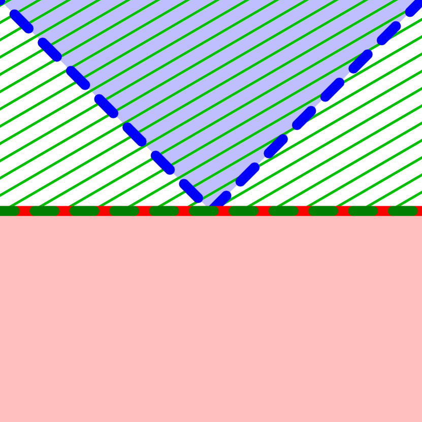
Input 1

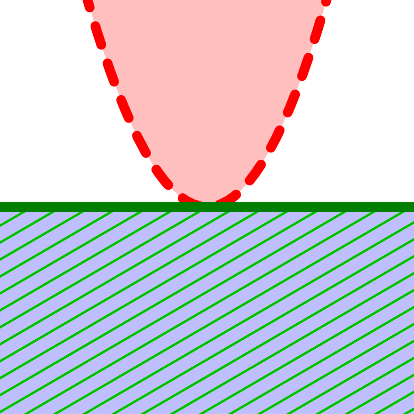
Input 2

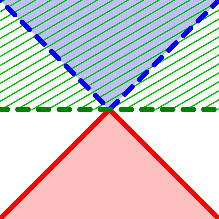
Input 3

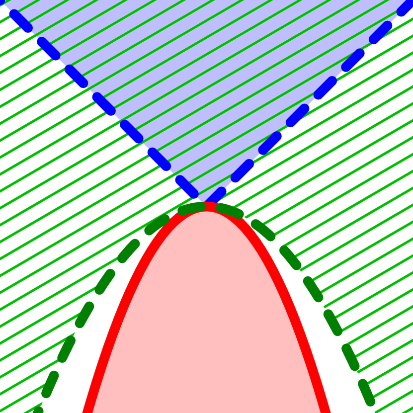
Input 4

Input 5

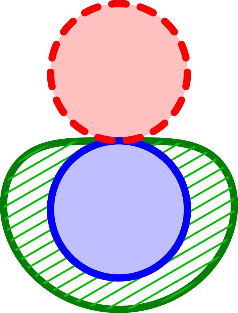
Input 7

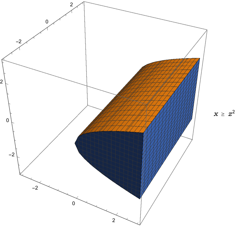
Input 8, $\cal T$

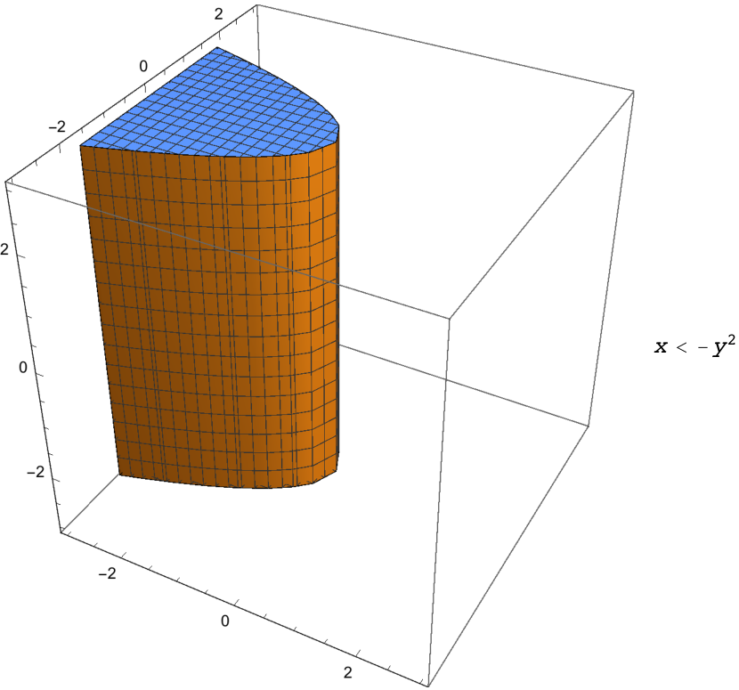
Input 8, ${\cal T}^{\prime}$

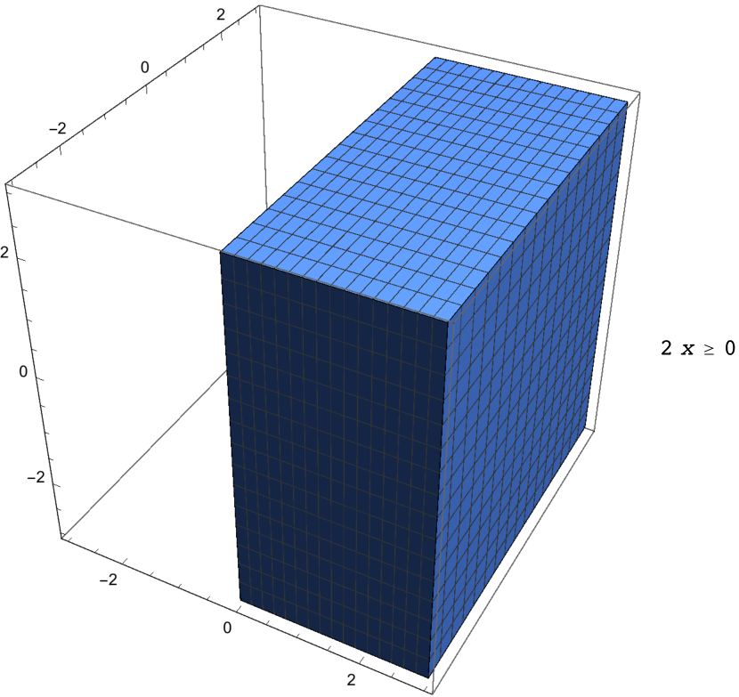
Input 8, $\cal S$

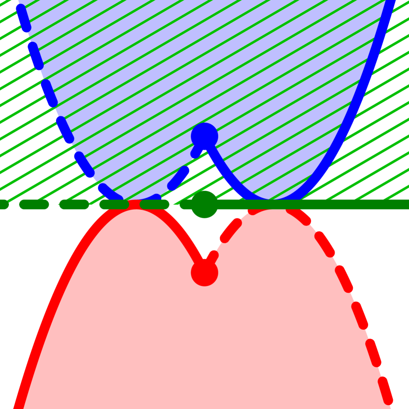
Input 9

Figure 2: Interpolants from Table 1. The blue, orange and green areas are for $\mathcal{T}$, $\mathcal{T}^{\prime}$, $\mathcal{S}$, respectively.

Listing 1: Code 1.3 of [8]

⬇

1real x,y;

2real xa = 0;

3real ya = 0;

4while(nondet()){

5 x = xa + 2*ya;

6 y = -2*xa + ya;

7 x++;

8 if(nondet()){

9 y = y + x;

10 }else{

11 y = y - x;

12 }

13 xa = x - 2*y;

14 ya = 2*x + y;

15}

16assert(xa + 2*ya >= 0);

Listing 2: Constant Acceleration

⬇

1real x,v;

2(x, v) = (0, 0);

3while(nondet()){

4 (x, v) = (x+2*v, v+2);

5}

6 assert(x >= 0);

$${\cal T}=\left(\begin{array}[]{l}(xa)+2(ya)\geq 0,\enspace x=(xa)+2(ya),\\ y=-2(xa)+(ya),\enspace x_{1}=x+1,\\ y_{1}=x_{1}+y,\enspace(xa_{1})=x_{1}-2y_{1},\\ (ya_{1})=2x_{1}+y_{1}\end{array}\right)$$

Figure 3: The SAS for an execution of the code in Listing 1

Program Verification Example I: Infeasibility Checking Consider the code in Listing 1; this is from [8, §7]. We shall solve Subproblem 1 in [8, §7]: if the property $(xa)+2(ya)\geq 0$ holds at Line 5, then it holds too after the execution along $5\rightarrow 6\rightarrow 7\rightarrow 8\rightarrow 9\rightarrow 13\rightarrow 14$. The execution is expressed as the SAS $\mathcal{T}$ in Fig. 3. Then our goal is to show that the negation ${\cal T}^{\prime}=\left((xa_{1})+2(ya_{1})<0\right)$ of the desired property is disjoint from $\mathcal{T}$.

Our tool yields $\mathcal{S}=\bigl{(}8-14(ya_{1})-7(xa_{1})\geq 0\bigr{)}$ as an interpolant of these $\mathcal{T}$ and $\mathcal{T}^{\prime}$ (in 14.1 seconds, with parameters $b=0,c=3$ and depth $d=11$). The interpolant witnesses disjointness. Our interpolant is far simpler than the interpolant given in [8].

Here the simplicity of our interpolant brings robustness as its benefit. Consider the other path $5\rightarrow\cdots\rightarrow 8\rightarrow 11\rightarrow 13\rightarrow 14$ of execution from Line $5$ to $14$, and let $\mathcal{T}_{0}$ be the SAS that expresses the execution. It turns out that our interpolant $\mathcal{S}$ in the above is at the same time an interpolant of $\mathcal{T}_{0}$ and $\mathcal{T}^{\prime}$. Thus our algorithm has managed, aiming at simpler interpolants, to automatically discover $-14(ya)-7(xa)$ (that is, $(xa)+2(ya)$) as a value that is significant regardless of the choice made in Line 8.

Program Verification Example II: CEGAR This is the example we discussed in Example 1.4. Here we provide further details, aiming at readers familiar with CEGAR.

One of the most important applications of interpolation in verification is in counterexample-guided abstraction refinement (CEGAR) [4]. There an interpolant $\mathcal{S}$ is used as (a candidate for) the “essential reason” to distinguish positive examples $\mathcal{T}$ from negative counterexamples $\mathcal{T}^{\prime}$.

As an example let us verify Listing 1 by CEGAR. Starting from the empty set of abstraction predicates, CEGAR would find the path $p_{1}:=(1\rightarrow 2\rightarrow 3\rightarrow 4\rightarrow 16)$ as a counterexample. This counterexample path turns out to be spurious: let $\mathcal{T}:=(xa=0,ya=0)$ express the path and $\mathcal{T^{\prime}}:=((xa)+2(ya)<0)$ express the negation of the assertion; our tool SSInt yields $189346(xa)+378692(ya)\geq 0$ (i.e. $(xa)+2(ya)\geq 0$) as an interpolant, proving their disjointness. For the interpolation the tool SSInt took $4.32$ seconds; we used the parameters $b=0$ and $c=5$.

Consequently we add $(xa)+2(ya)\geq 0$ as a new abstraction predicate and run the CEGAR loop again. This second run succeeds, since $(xa)+2(ya)\geq 0$ turns out to be a suitable invariant for the loop in Line 4. We conclude safety of Listing 1.

We tried to do the same with the tool $\mathtt{aiSat}$ [6, 8] instead of our SSInt. It does not succeed in interpolating $\mathcal{T}=(xa=0,ya=0)$ and $\mathcal{T^{\prime}}=((xa)+2(ya)<0)$, since sharpness is required here (Prop. 3.3). As a workaround we tried strengthening $\mathcal{T^{\prime}}=((xa)+2(ya)<0)$ into $\mathcal{T}^{\prime}_{0}=((xa)+2(ya)\leq-10^{-7})$; $\mathtt{aiSat}$ then succeeded and yielded an interpolant $\mathcal{S}=(137.3430+5493721088(ya)+2746860544(xa)>0)$. This predicate, however, cannot exclude the spurious path $p_{1}$ because $\mathcal{S}$ and the negation $(xa)+2(ya)<0$ of the assertion are satisfiable with $xa=0$ and $ya=-1.25\times 10^{-8}$.

Program Verification Example III: CEGAR Here is another CEGAR example. Consider the code in Listing 2 that models movement with constant acceleration. We initially have the empty set of abstraction predicates. After the first run of the CEGAR loop we would obtain a counterexample path $p_{1}:=(1\rightarrow 2\rightarrow 3\rightarrow 6)$; note that, since there are no predicates yet, $x$ can be anything and thus the assertion may fail.

We let $\mathcal{T}_{1}:=(x=0,v=0)$ express the counterexample $p_{1}$ and $\mathcal{T}^{\prime}_{1}:=(x<0)$ express the negation of the assertion. For these $\mathcal{T}_{1},\mathcal{T}^{\prime}_{1}$ our tool SSInt synthesizes $\mathcal{S}_{1}:=(2x\geq 0)$ as their interpolant (in $1.92$ seconds, with $b=0$, $c=5$, and $d=1$).

Thus we add $2x\geq 0$ as an abstraction predicate and run the CEGAR loop again. We would then find the path $p_{2}:=(1\rightarrow 2\rightarrow 3\rightarrow 4\rightarrow 5\rightarrow 6)$ as a counterexample—note that the previous counterexample $p_{1}$ is successfully excluded by the new predicate $2x\geq 0$. Much like before, we let $\mathcal{T}_{2}:=(v_{1}=0)$ express an initial segment of the path $p_{2}$ and let $\mathcal{T}_{2}^{\prime}:=(x_{1}=0,v_{2}=v_{1}+2,x_{2}=x_{1}+2v_{1},x_{2}<0)$ express the rest of the path $p_{2}$ (together with the negation of the assertion), and we shall look for their interpolant $\mathcal{S}_{2}$ as the witness of infeasibility of the path $p_{2}$. SSInt succeeds, yielding $\mathcal{S}_{2}:=(8v_{1}\geq 0)$ in $2.87$ seconds with $b=0,c=5,d=1$.

In the third run of the CEGAR loop we use both $2x\geq 0$ and $8v\geq 0$ (from $\mathcal{S}_{1},\mathcal{S}_{2}$) as abstraction predicates. The proof then succeeds and we conclude safety of Listing 2.

We did not succeed in doing the same with $\mathtt{aiSat}$. In the first CEGAR loop an interpolant of $\mathcal{T}_{1}$ and $\mathcal{T}_{1}^{\prime}$ cannot be computed because it has to be sharp. As we did in the previous example we could strengthen $\mathcal{T}_{1}^{\prime}$ to $\mathcal{T}_{1}^{\prime\prime}:=(x\leq 10^{-7})$ and use an interpolant of $\mathcal{T}_{1}$ and $\mathcal{T}_{1}^{\prime\prime}$ instead for the next iteration. $\mathtt{aiSat}$ generated an interpolant $3790.1050+75802091520.0000x>0$ of $\mathcal{T}_{1}$ and $\mathcal{T}_{1}^{\prime\prime}$; however this fails to exclude the spurious counterexample path $p_{1}$.

Overall this example demonstrates that sharpness of interpolants can be a decisive issue in their application in program verification.

Acknowledgments

Thanks are due to Eugenia Sironi, Gidon Ernst and the anonymous referees for their useful comments. T.O., K. Kido and I.H. are supported by JST ERATO HASUO Metamathematics for Systems Design Project (No. JPMJER1603), and JSPS Grants-in-Aid No. 15KT0012 & 15K11984. K. Kojima is supported by JST CREST. K.S. is supported by JST PRESTO No. JPMJPR15E5 and JSPS Grants-in-Aid No. 15KT0012. K. Kido is supported by JSPS Grant-in-Aid for JSPS Research Fellows No. 15J05580.

Appendix 0.A Omitted Proofs

0.A.1 Proof of Lem. 2.9

Definition 0.A.1 (quadratic module)

A quadratic module generated by $M=(m_{\lambda})_{\lambda\in\Lambda}\in\real[\vec{X}]^{\Lambda}$ ($\Lambda$ is an index set) is the set

$$\mathcal{QM}(M)\coloneqq\Set{q+\sum_{\lambda\in\Lambda}q_{\lambda}m_{\lambda}}{\begin{aligned} &\text{$q\in\mathcal{C}(\emptyset)$, $(q_{\lambda})_{\lambda\in\Lambda}\in\mathcal{C}(\emptyset)^{\Lambda}$, and}\\ &\text{$q_{\lambda}=0$ except for finitely many $\lambda$'s}\end{aligned}}.$$ (33)

Lem. 2.9 is an immediate consequence of the following lemma.

Lemma 0.A.2

Let $f_{1},\dots,f_{s}\in\real[\vec{X}]$. Then,

$$\mathcal{C}(f_{1},\dots,f_{s})=\mathcal{QM}(f_{1}^{i_{1}}\dotsm f_{s}^{i_{s}}\mid i\in\mathbf{2}^{s})$$ (34)

where $i=(i_{1},\dots,i_{s})$.

Proof

The left-to-right direction is proved by induction on the construction of $\mathcal{C}(f_{1},\dots,f_{s})$. Let $f\in\mathcal{C}(f_{1},\dots,f_{s})$.

1. Case: $f=f_{\lambda}$ for some $\lambda=1,\dots,s$.

   $$f=f_{\lambda}=f_{1}^{0}\dotsm f_{\lambda}^{1}\dotsm f_{s}^{0}\in\mathcal{QM}(f_{1}^{i_{1}}\dotsm f_{s}^{i_{s}}\mid i\in\mathbf{2}^{s}).$$ (35)

2. Case: $f=g^{2}$ for some $g\in\real[\vec{X}]$.

   $$f=g^{2}\in\mathcal{QM}(f_{1}^{i_{1}}\dotsm f_{s}^{i_{s}}\mid i\in\mathbf{2}^{s}).$$ (36)

3. Case: $f=g+h$ for some $g,h\in\mathcal{C}(f_{1},\dots,f_{s})\cap\mathcal{QM}(f_{1}^{i_{1}}\dotsm f_{s}^{i_{s}}\mid i\in\mathbf{2}^{s})$. Obvious, because $\mathcal{QM}(f_{1}^{i_{1}}\dotsm f_{s}^{i_{s}}\mid i\in\mathbf{2}^{s})$ is closed under addition.

4. Case: $f=gh$ for some $g,h\in\mathcal{C}(f_{1},\dots,f_{s})\cap\mathcal{QM}(f_{1}^{i_{1}}\dotsm f_{s}^{i_{s}}\mid i\in\mathbf{2}^{s})$. $g$ and $h$ have the form

   $$g=\sum_{i\in\mathbf{2}^{s}}q_{i}f_{1}^{i_{1}}\dotsm f_{s}^{i_{s}},\quad h=\sum_{j\in\mathbf{2}^{s}}r_{j}f_{1}^{j_{1}}\dotsm f_{s}^{j_{s}},$$ (37)

   where $q_{i},r_{j}\in\mathcal{C}(\emptyset)$. Let $p_{\lambda}=\sum_{i+j=\lambda}q_{i}r_{j}\in\mathcal{C}(\emptyset)$. Then

   $$gh =\sum_{i\in\mathbf{2}^{s}}\sum_{j\in\mathbf{2}^{s}}q_{i}r_{j}f_{1}^{i_{1}+j_{1}}\dotsm f_{s}^{i_{s}+j_{s}}$$ (38)

   $$=\sum_{\lambda\in\mathbf{2}^{s}}\sum_{i+j=\lambda}q_{i}r_{j}f_{1}^{\lambda_{1}}\dotsm f_{s}^{\lambda_{s}}$$ (39)

   $$=\sum_{\lambda\in\mathbf{2}^{s}}p_{\lambda}f_{1}^{\lambda_{1}}\dotsm f_{s}^{\lambda_{s}}$$ (40)

   $$=\sum_{\lambda\in\mathbf{2}^{s}}\left(p_{\lambda}f_{1}^{2\lfloor\lambda_{1}/2\rfloor}\dotsm f_{s}^{2\lfloor\lambda_{s}/2\rfloor}\right)f_{1}^{\lambda_{1}\bmod 2}\dotsm f_{s}^{\lambda_{s}\bmod 2}.$$ (41)

   Because $p_{\lambda}f_{1}^{2\lfloor\lambda_{1}/2\rfloor}\dotsm f_{s}^{2\lfloor\lambda_{s}/2\rfloor}\in\mathcal{C}(\emptyset)$ for each $\lambda\in 2^{s}$, we have $f=gh\in\mathcal{QM}(f_{1}^{i_{1}}\dotsm f_{s}^{i_{s}}\mid i\in\mathbf{2}^{s})$.

For the converse, let $f\in\mathcal{QM}(f_{1}^{i_{1}}\dotsm f_{s}^{i_{s}}\mid i\in\mathbf{2}^{s})$. Then $f$ has the form $f=\sum_{i\in\mathbf{2}^{s}}q_{i}f_{1}^{i_{1}}\dotsm f_{s}^{i_{s}}$ where $q_{i}\in\mathcal{C}(\emptyset)\subseteq\mathcal{C}(f_{1},\dots,f_{s})$. Then $f$ indeed belongs to $\mathcal{C}(f_{1},\dots,f_{s})$, because cones are closed under addition and multiplication. ∎

0.A.2 Proof of Prop. 3.3

We argue by contradiction. Assume that there exist polynomials $\widetilde{f},g,\widetilde{h}$ that satisfy the conditions in the proposition. By the feasibility assumption there exists some $\vec{r}\in\llbracket\mathcal{T}_{\bullet}\rrbracket\cap\llbracket\mathcal{T}^{\prime}_{\bullet}\rrbracket$. For this $\vec{r}$ we have $\widetilde{f}(\vec{r})+\widetilde{h}(\vec{r})\geq 0$ by Lem. 2.3, while by $1+\widetilde{f}+g^{2}+\widetilde{h}=0$ we have $\widetilde{f}(\vec{r})+\widetilde{h}(\vec{r})=-1-\bigl{(}g(\vec{r})\bigr{)}^{2}<0$. Contradiction.

0.A.3 Proof of Thm. 3.7

The “if” direction is easy. Suppose there exist such polynomials $f,g,h$ as required. Assume $\vec{r}\in\llbracket\mathcal{T}\rrbracket$; then we have $f(\vec{r})\geq 0$, $g(\vec{r})>0$, and $h(\vec{r})=0$ by Lem. 2.3 and 3.6. Thus we have $f(\vec{r})+g(\vec{r})+h(\vec{r})>0$, which contradicts with $f+g+h=0$. Therefore $\llbracket\mathcal{T}\rrbracket=\emptyset$.

For the “only if” direction we rely on Thm. 2.4, via the translation of $\text{SAS}_{<}$’s to SAS_≠’s that we described after Def. 3.4, and use the fact that $\mathcal{M}(g_{1},\dots,g_{t})\subseteq\mathcal{SC}(g_{1},\dots,g_{t})$. ∎

0.A.4 Proof of Lem. 3.12

We introduce a notion similar to quadratic module to represent strict cones.

Definition 0.A.3 (positive module)

An positive module generated by $M=(m_{\lambda})_{\lambda\in\Lambda}\in\real[\vec{X}]^{\Lambda}$ ($\Lambda$ is an index set) is the set

$$\mathcal{PM}(M)\coloneqq\Set{r+\sum_{\lambda\in\Lambda}r_{\lambda}m_{\lambda}}{\begin{aligned} &\text{$r\in{}_{\geq 0}$, $(r_{\lambda})_{\lambda\in\Lambda}\in{}_{\geq 0}^{\Lambda}$,}\\ &\text{$r_{\lambda}=0$ except for finitely many $\lambda$'s, and}\\ &\text{either $r_{\lambda}>0$ for at least one $\lambda$, or $r>0$}\end{aligned}}.$$ (42)

Then Lem. 3.12 is an immediate consequence of the following lemma.

Lemma 0.A.4

Let $f_{1},\dots,f_{s}\in\real[\vec{X}]$. Then,

$$\mathcal{SC}(f_{1},\dots,f_{s})=\mathcal{PM}(f_{1}^{i_{1}}\dotsm f_{s}^{i_{s}}\mid i\in\mathbb{N}^{s}).$$ (43)

Proof

The left-to-right direction is proved by induction on the construction of $\mathcal{SC}(f_{1},\dots,f_{s})$. Let $f\in\mathcal{SC}(f_{1},\dots,f_{s})$.

1. Case: $f=f_{\lambda}$ for some $\lambda=1,\dots,s$.

   $$f=f_{\lambda}=f_{1}^{0}\dotsm f_{\lambda}^{1}\dotsm f_{s}^{0}\in\mathcal{PM}(f_{1}^{i_{1}}\dotsm f_{s}^{i_{s}}\mid i\in\mathbb{N}^{s}).$$ (44)

2. Case: $f=r$ for some $r\in{}_{>0}$.

   $$f=r\in\mathcal{PM}(f_{1}^{i_{1}}\dotsm f_{s}^{i_{s}}\mid i\in\mathbb{N}^{s}).$$ (45)

3. Case: $f=g+h$ for some $g,h\in\mathcal{SC}(f_{1},\dots,f_{s})\cap\mathcal{PM}(f_{1}^{i_{1}}\dotsm f_{s}^{i_{s}}\mid i\in\mathbb{N}^{s})$. Obvious, because $\mathcal{PM}(f_{1}^{i_{1}}\dots f_{s}^{i_{s}}\mid i\in\mathbb{N}^{s})$ is closed under addition.

4. Case: $f=gh$ for some $g,h\in\mathcal{SC}(f_{1},\dots,f_{s})\cap\mathcal{PM}(f_{1}^{i_{1}}\dotsm f_{s}^{i_{s}}\mid i\in\mathbb{N}^{s})$. $g$ and $h$ have the form of

   $$g=\sum_{i\in\mathbb{N}^{s}}r_{i}f_{1}^{i_{1}}\dotsm f_{s}^{i_{s}},\quad h=\sum_{j\in\mathbb{N}^{s}}r^{\prime}_{j}f_{1}^{j_{1}}\dotsm f_{s}^{j_{s}},$$ (46)

   where $r_{i},r^{\prime}_{j}\in{}_{\geq 0}$. Let $q_{\lambda}=\sum_{i+j=\lambda}r_{i}r^{\prime}_{j}$. Then obviously there are only finitely many $\lambda$ such that $q_{\lambda}>0$. Moreover, there exists $\lambda$ such that $q_{\lambda}>0$. Indeed, for $i$ and $j$ such that $r_{i},r^{\prime}_{j}>0$, we have

   $$q_{i+j}=\sum_{i^{\prime}+j^{\prime}=i+j}r_{i^{\prime}}r^{\prime}_{j^{\prime}}\geq r_{i}r^{\prime}_{j}>0.$$ (47)

   Therefore,

   $$gh =\sum_{i\in\mathbb{N}^{s}}\sum_{j\in\mathbb{N}^{s}}r_{i}r^{\prime}_{j}f_{1}^{i_{1}+j_{1}}\dotsm f_{s}^{i_{s}+j_{s}}$$ (48)

   $$=\sum_{\lambda\in\mathbb{N}^{s}}\sum_{i+j=\lambda}r_{i}r^{\prime}_{j}f_{1}^{i_{1}+j_{1}}\dotsm f_{s}^{i_{s}+j_{s}}$$ (49)

   $$=\sum_{\lambda\in\mathbb{N}^{s}}q_{\lambda}f_{1}^{\lambda_{1}}\dotsm f_{s}^{\lambda_{s}}$$ (50)

   $$\in\mathcal{PM}(f_{1}^{i_{1}}\dotsm f_{s}^{i_{s}}\mid i\in\mathbb{N}^{s}).$$ (51)

For the converse, let us consider $f=r+\sum_{i}r_{i}f_{1}^{i_{1}}\dotsm f_{s}^{i_{s}}\in\mathcal{PM}(f_{1}^{i_{1}}\dotsm f_{s}^{i_{s}}\mid i\in\mathbb{N}^{s})$. For each $i$ such that $r_{i}>0$, we have $r_{i},f_{1}^{i_{1}},\dots,f_{s}^{i_{s}}\in\mathcal{SC}(f_{1},\dots,f_{s})$. Moreover, either $r>0$ or there exists at least one such $i$. Therefore we conclude that $f\in\mathcal{SC}(f_{1},\dots,f_{s})$, because strict cones are closed under addition and multiplication. ∎

0.A.5 Proof of Lem. 4.1

We first notice that in case where the output of $\mathsf{CFE}(r,d-1)$ in Line 10 equals $r$, then we can check that the value of $y$ at Line 11 equals $x$ by a straightforward calculation.

We can prove the lemma by induction on $\max\{x_{i}\mid 1\leq i\leq n\}$. We check several cases in turn.

1. In the case where there is only one nonzero element in $x$, set $M=1$. For simplicity, we consider the case $x=(k,0,0)$. Then $p=1$ and $a=(1,0,0)$. Therefore if $d=1$, then $y=a=x$ (as ratios). If $d>1$, then $r=(k,0,0)$, so by induction on $d$ we obtain $r^{\prime}=r$, and thus $y=x$ by the remark above.

2. In the case where there are more than one nonzero elements, and all of them are the same, set $M=2$. For simplicity, we consider the case $x=(k,k,k,0,0)$. Then $p=1$ and $a=(1,1,1,0,0)$. If $d\geq M=2$, then else-branch is taken, and $r=(k,0,0,0,0)$. By the previous case, we have $r^{\prime}=r$. Therefore $y=x$ by the remark.

3. In other cases, let $r$ as in Line 9, and $M$ be the depth $d$ for which $\mathsf{CFE}(r,d)$ stabilizes (such $M$ exists by the induction hypothesis). Then for any $d\geq M+1$ we have $r^{\prime}=r$, and thus $y=x$ by the remark.

The second claim is obvious from the construction of the algorithm.

Appendix 0.B Topological and Algebraic Closure

Let us consider the difference between topological closure and algebraic closure, that is, the difference between $\llbracket\mathcal{T}_{\bullet}\rrbracket\subseteq{}^{k}$ (where $\mathcal{T}_{\bullet}$ is from Def. 3.1) and $\overline{\llbracket\mathcal{T}\rrbracket}\subseteq{}^{k}$. Here $\overline{(\underline{\phantom{n}}\,)}$ refers to the closure with respect to the Euclidean topology of ^k.

They coincide in many cases but do not always. For example, for $\mathcal{T}=(x^{3}-2x^{2}+x\leq 0,x^{3}-2x^{2}+x\neq 0)$, we have $\llbracket\mathcal{T}_{\bullet}\rrbracket=\llbracket x^{3}-2x^{2}+x\leq 0\rrbracket=(-\infty,0]\cup\set{1}$, but $\overline{\llbracket\mathcal{T}\rrbracket}=\overline{(-\infty,0)}=(-\infty,0]$.

We can show the following inclusion in general.

Proposition 0.B.1

Let $\mathcal{A}=(f_{1}\triangleright_{1}0,\dots,f_{n}\triangleright_{n}0)$ be an SAS_≠, where $\triangleright_{i}\in\{\geq,\neq,=\}$. Then

$$\overline{\llbracket\mathcal{A}\rrbracket}\subseteq\llbracket\mathcal{A}_{\bullet}\rrbracket.$$ (52)

Proof

The proof is by induction on $n$.

• Base cases: The cases $\triangleright_{1}=(=)$ and $\triangleright_{1}=(\geq)$ are easy because $f_{1}$ is continuous and both $\set{0}$ and $[0,\infty)$ are closed in . For the remaining case where $\triangleright_{1}=(\neq)$, we have $\overline{\llbracket f_{1}\neq 0\rrbracket}\subseteq{}^{k}=\llbracket()\rrbracket=\llbracket\mathcal{A}_{\bullet}\rrbracket$.

• Step case: Let $\mathcal{B}=(f_{1}\triangleright_{1}0,\dots,f_{n}\triangleright_{n}0)$.

  $$\overline{\llbracket\mathcal{A}\rrbracket} =\overline{\llbracket\mathcal{B},f_{n+1}\triangleright_{n+1}0\rrbracket}$$

  $$=\overline{\llbracket\mathcal{B}\rrbracket\cap\llbracket f_{n+1}\triangleright_{n+1}0\rrbracket}$$

  $$\subseteq\overline{\llbracket\mathcal{B}\rrbracket}\cap\overline{\llbracket f_{n+1}\triangleright_{n+1}0\rrbracket}$$

  $$\subseteq\llbracket\mathcal{B}_{\bullet}\rrbracket\cap\llbracket(f_{n+1}\triangleright_{n+1}0)_{\bullet}\rrbracket$$

  (by the induction hypothesis and arguments similar to the base case)

  $$=\llbracket\mathcal{A}_{\bullet}\rrbracket.$$ ∎

It follows that $\overline{\llbracket\mathcal{T}\rrbracket}\cap\overline{\llbracket\mathcal{T}^{\prime}\rrbracket}\subseteq\llbracket\mathcal{T}_{\bullet}\rrbracket\cap\llbracket\mathcal{T}^{\prime}_{\bullet}\rrbracket$. The opposite inclusion fails in general: for $\mathcal{T}=(x^{3}-2x^{2}+x\leq 0,x^{3}-2x^{2}+x\neq 0),\mathcal{T^{\prime}}=(x\geq 0)$, $\overline{\llbracket\mathcal{T}\rrbracket}\cap\overline{\llbracket\mathcal{T}^{\prime}\rrbracket}=(-\infty,0)\cap[0,\infty)=\emptyset$ and $\llbracket\mathcal{T}_{\bullet}\rrbracket\cap\llbracket\mathcal{T}^{\prime}_{\bullet}\rrbracket=((-\infty,0)\cup\set{1})\cap[0,\infty)=\set{1}$.

Appendix 0.C Relationship of the Two Algorithms

We show that if Algorithm 1 generates an interpolant for two SAS_≠’s, then Algorithm 2 generates an interpolant for two $\text{SAS}_{<}$’s that are equivalent to those two SAS_≠’s.

Proposition 0.C.1

Let $\mathcal{T}$ and $\mathcal{T}^{\prime}$ be the SAS_≠’s in (8). Let $\mathcal{U}$ and $\mathcal{U}^{\prime}$ be the following $\text{SAS}_{<}$’s.

$$\footnotesize\begin{split}\mathcal{U}&=\left(\begin{array}[]{l}f_{1}(\vec{X},\vec{Y})\geq 0\enspace,\;\dotsc,\;f_{s}(\vec{X},\vec{Y})\geq 0\enspace,\quad g^{2}_{1}(\vec{X},\vec{Y})>0\enspace,\;\dotsc,\;g^{2}_{t}(\vec{X},\vec{Y})>0\enspace,\\ h_{1}(\vec{X},\vec{Y})=0\enspace,\;\dotsc,\;h_{u}(\vec{X},\vec{Y})=0\end{array}\right),\\ \mathcal{U}^{\prime}&=\left(\begin{array}[]{l}f^{\prime}_{1}(\vec{X},\vec{Z})\geq 0\enspace,\;\dotsc,\;f^{\prime}_{s^{\prime}}(\vec{X},\vec{Z})\geq 0\enspace,\quad{g^{\prime}}^{2}_{1}(\vec{X},\vec{Z})>0\enspace,\;\dotsc,\;{g^{\prime}}^{2}_{t^{\prime}}(\vec{X},\vec{Z})>0\enspace,\\ h^{\prime}_{1}(\vec{X},\vec{Z})=0\enspace,\;\dotsc,\;h^{\prime}_{u^{\prime}}(\vec{X},\vec{Z})=0\end{array}\right).\end{split}$$ (53)

Obviously we have $\llbracket\mathcal{T}\rrbracket=\llbracket\mathcal{U}\rrbracket$ and $\llbracket\mathcal{T}^{\prime}\rrbracket=\llbracket\mathcal{U}^{\prime}\rrbracket$.

Assume there exist polynomials $f,f^{\prime},g,h,h^{\prime}$ that satisfy the following conditions (cf. Thm. 2.7).

• $f\in\mathcal{C}(f_{1},\dots,f_{s}),f^{\prime}\in\mathcal{C}(f^{\prime}_{1},\dots,f^{\prime}_{s^{\prime}}),g\in\mathcal{M}(g_{1},\dots,g_{t},g^{\prime}_{1},\dots,g^{\prime}_{t^{\prime}}),h\in\mathcal{I}(h_{1},\dots,h_{u})$, $h^{\prime}\in\mathcal{I}(h^{\prime}_{1},\dots,h^{\prime}_{u^{\prime}})$, and

• $1+f+f^{\prime}+g^{2}+h+h^{\prime}=0$.

Then there exist polynomials $\widetilde{f},\widetilde{f}^{\prime},\widetilde{g},\widetilde{h},\widetilde{h}^{\prime}$ that satisfy the following (cf. Thm. 3.8).

• $\widetilde{f}\in\mathcal{C}(f_{1},\dots,f_{s},g_{1}^{2},\dots,g_{t}^{2}),\widetilde{f}^{\prime}\in\mathcal{C}(f^{\prime}_{1},\dots,f^{\prime}_{s},{g^{\prime}}_{1}^{2},\dots,{g^{\prime}}_{t}^{2}),\widetilde{g}\in\mathcal{SC}(g^{2}_{1},\dots,g^{2}_{t}),\widetilde{h}\in\mathcal{I}(h_{1},\dots,h_{u}),\widetilde{h}^{\prime}\in\mathcal{I}(h^{\prime}_{1},\dots,h^{\prime}_{u^{\prime}})$ and

• $\widetilde{f}+\widetilde{f}^{\prime}+\widetilde{g}+\widetilde{h}+\widetilde{h}^{\prime}=0$.

Proof

Set

$$\widetilde{f}=g^{2}+f\enspace,\quad\widetilde{f}^{\prime}=f^{\prime}\enspace,\quad\widetilde{g}=1\enspace,\quad\widetilde{h}=h\enspace,\quad\widetilde{h}^{\prime}=h^{\prime}\enspace.$$ (54)

The equality $\widetilde{f}+\widetilde{f}^{\prime}+\widetilde{g}+\widetilde{h}+\widetilde{h}^{\prime}=0$ is easy. Because $g^{2}$ is an SOS and $f\in\mathcal{C}(f_{1},\dots,f_{s})$, $\widetilde{f}\in\mathcal{C}(f_{1},\dots,f_{s},g_{1}^{2},\dots,g_{t}^{2})$ hold. $\widetilde{f}^{\prime}\in\mathcal{C}(f^{\prime}_{1},\dots,f^{\prime}_{s},{g^{\prime}}_{1}^{2},\dots,{g^{\prime}}_{t}^{2})$ is obvious. By the definition of strict cone, $\widetilde{g}=1\in\mathcal{SC}(g_{1},\dots,g_{t})$. $\widetilde{h}\in\mathcal{I}(h_{1},\dots,h_{u}),\widetilde{h}^{\prime}\in\mathcal{I}(h^{\prime}_{1},\dots,h^{\prime}_{u^{\prime}})$ are obvious. ∎

Recall that Algorithm 1 generates an interpolant based on Thm. 2.7, and that Algorithm 2 is based on Thm. 3.8. Therefore by Prop. 0.C.1, if the former succeeds, so does the latter.

References

- [1] Anai, H., Parrilo, P.A.: Convex quantifier elimination for semidefinite programming. In: Proceedings of the International Workshop on Computer Algebra in Scientific Computing, CASC (2003)
- [2] Besson, F.: Fast reflexive arithmetic tactics the linear case and beyond. In: Altenkirch, T., McBride, C. (eds.) Types for Proofs and Programs, International Workshop, TYPES 2006, Nottingham, UK, April 18-21, 2006, Revised Selected Papers. Lecture Notes in Computer Science, vol. 4502, pp. 48–62. Springer (2006), https://doi.org/10.1007/978-3-540-74464-1_4
- [3] Bochnak, J., Coste, M., Roy, M.F.: Real algebraic geometry. Springer (1999)
- [4] Clarke, E.M., Grumberg, O., Jha, S., Lu, Y., Veith, H.: Counterexample-guided abstraction refinement for symbolic model checking. J. ACM 50(5), 752–794 (2003), http://doi.acm.org/10.1145/876638.876643
- [5] Colón, M., Sankaranarayanan, S., Sipma, H.: Linear invariant generation using non-linear constraint solving. In: Hunt Jr. and Somenzi [14], pp. 420–432
- [6] Dai, L.: The tool , github.com/djuanbei/aiSat, cloned on January 17th, 2017.
- [7] Dai, L., Gan, T., Xia, B., Zhan, N.: Barrier certificates revisited. J. Symb. Comput. 80, 62–86 (2017), http://dx.doi.org/10.1016/j.jsc.2016.07.010
- [8] Dai, L., Xia, B., Zhan, N.: Generating non-linear interpolants by semidefinite programming. In: Sharygina, N., Veith, H. (eds.) Computer Aided Verification - 25th International Conference, CAV 2013, Saint Petersburg, Russia, July 13-19, 2013. Proceedings. Lecture Notes in Computer Science, vol. 8044, pp. 364–380. Springer (2013), http://dx.doi.org/10.1007/978-3-642-39799-8_25
- [9] Gan, T., Dai, L., Xia, B., Zhan, N., Kapur, D., Chen, M.: Interpolant synthesis for quadratic polynomial inequalities and combination with EUF. In: Olivetti, N., Tiwari, A. (eds.) Automated Reasoning - 8th International Joint Conference, IJCAR 2016, Coimbra, Portugal, June 27 - July 2, 2016, Proceedings. Lecture Notes in Computer Science, vol. 9706, pp. 195–212. Springer (2016), https://doi.org/10.1007/978-3-319-40229-1_14
- [10] Gao, S., Zufferey, D.: Interpolants in nonlinear theories over the reals. In: Chechik, M., Raskin, J. (eds.) Tools and Algorithms for the Construction and Analysis of Systems - 22nd International Conference, TACAS 2016, Held as Part of the European Joint Conferences on Theory and Practice of Software, ETAPS 2016, Eindhoven, The Netherlands, April 2-8, 2016, Proceedings. Lecture Notes in Computer Science, vol. 9636, pp. 625–641. Springer (2016), https://doi.org/10.1007/978-3-662-49674-9_41
- [11] Gurfinkel, A., Rollini, S.F., Sharygina, N.: Interpolation properties and sat-based model checking. In: Hung, D.V., Ogawa, M. (eds.) Automated Technology for Verification and Analysis - 11th International Symposium, ATVA 2013, Hanoi, Vietnam, October 15-18, 2013. Proceedings. Lecture Notes in Computer Science, vol. 8172, pp. 255–271. Springer (2013)
- [12] Harrison, J.: Verifying nonlinear real formulas via sums of squares. In: Schneider, K., Brandt, J. (eds.) Theorem Proving in Higher Order Logics, 20th International Conference, TPHOLs 2007, Kaiserslautern, Germany, September 10-13, 2007, Proceedings. Lecture Notes in Computer Science, vol. 4732, pp. 102–118. Springer (2007), https://doi.org/10.1007/978-3-540-74591-4_9
- [13] Henzinger, T.A., Jhala, R., Majumdar, R., McMillan, K.L.: Abstractions from proofs. In: Jones, N.D., Leroy, X. (eds.) Proceedings of the 31st ACM SIGPLAN-SIGACT Symposium on Principles of Programming Languages, POPL 2004, Venice, Italy, January 14-16, 2004. pp. 232–244. ACM (2004), http://dl.acm.org/citation.cfm?id=964001
- [14] Hunt Jr., W.A., Somenzi, F. (eds.): Computer Aided Verification, 15th International Conference, CAV 2003, Boulder, CO, USA, July 8-12, 2003, Proceedings, Lecture Notes in Computer Science, vol. 2725. Springer (2003)
- [15] Jhala, R., McMillan, K.L.: Interpolant-based transition relation approximation. In: Etessami, K., Rajamani, S.K. (eds.) Computer Aided Verification, 17th International Conference, CAV 2005, Edinburgh, Scotland, UK, July 6-10, 2005, Proceedings. Lecture Notes in Computer Science, vol. 3576, pp. 39–51. Springer (2005)
- [16] Jhala, R., McMillan, K.L.: A practical and complete approach to predicate refinement. In: Hermanns, H., Palsberg, J. (eds.) Tools and Algorithms for the Construction and Analysis of Systems, 12th International Conference, TACAS 2006 Held as Part of the Joint European Conferences on Theory and Practice of Software, ETAPS 2006, Vienna, Austria, March 25 - April 2, 2006, Proceedings. Lecture Notes in Computer Science, vol. 3920, pp. 459–473. Springer (2006), https://doi.org/10.1007/11691372_33
- [17] Kaltofen, E., Li, B., Yang, Z., Zhi, L.: Exact certification of global optimality of approximate factorizations via rationalizing sums-of-squares with floating point scalars. In: Sendra, J.R., González-Vega, L. (eds.) Symbolic and Algebraic Computation, International Symposium, ISSAC 2008, Linz/Hagenberg, Austria, July 20-23, 2008, Proceedings. pp. 155–164. ACM (2008), http://doi.acm.org/10.1145/1390768.1390792
- [18] Kupferschmid, S., Becker, B.: Craig interpolation in the presence of non-linear constraints. In: Fahrenberg, U., Tripakis, S. (eds.) Formal Modeling and Analysis of Timed Systems - 9th International Conference, FORMATS 2011, Aalborg, Denmark, September 21-23, 2011. Proceedings. Lecture Notes in Computer Science, vol. 6919, pp. 240–255. Springer (2011)
- [19] Lang, S.: Introduction to Diophantine Approximations. Springer books on elementary mathematics, Springer (1995), http://dx.doi.org/10.1007/978-1-4612-4220-8
- [20] Lin, W., Wu, M., Yang, Z., Zeng, Z.: Proving total correctness and generating preconditions for loop programs via symbolic-numeric computation methods. Frontiers of Computer Science 8(2), 192–202 (2014), http://dx.doi.org/10.1007/s11704-014-3150-6
- [21] McMillan, K.L.: Interpolation and sat-based model checking. In: Hunt Jr. and Somenzi [14], pp. 1–13
- [22] McMillan, K.L.: Applications of craig interpolants in model checking. In: Halbwachs, N., Zuck, L.D. (eds.) Tools and Algorithms for the Construction and Analysis of Systems, 11th International Conference, TACAS 2005, Held as Part of the Joint European Conferences on Theory and Practice of Software, ETAPS 2005, Edinburgh, UK, April 4-8, 2005, Proceedings. Lecture Notes in Computer Science, vol. 3440, pp. 1–12. Springer (2005), http://dx.doi.org/10.1007/978-3-540-31980-1_1
- [23] McMillan, K.L.: Lazy abstraction with interpolants. In: Ball, T., Jones, R.B. (eds.) Computer Aided Verification, 18th International Conference, CAV 2006, Seattle, WA, USA, August 17-20, 2006, Proceedings. Lecture Notes in Computer Science, vol. 4144, pp. 123–136. Springer (2006), https://doi.org/10.1007/11817963_14
- [24] Parrilo, P.: Structured semidefinite programs and semialgebraic geometry methods in robustness and optimization. Ph.D. thesis, California Inst. of Tech. (2000)
- [25] Parrilo, P.A.: Semidefinite programming relaxations for semialgebraic problems. Mathematical Programming 96(2), 293–320 (2003), http://dx.doi.org/10.1007/s10107-003-0387-5
- [26] Peyrl, H., Parrilo, P.A.: Computing sum of squares decompositions with rational coefficients. Theor. Comput. Sci. 409(2), 269–281 (2008), https://doi.org/10.1016/j.tcs.2008.09.025
- [27] Platzer, A., Quesel, J., Rümmer, P.: Real world verification. In: Schmidt, R.A. (ed.) Automated Deduction - CADE-22, 22nd International Conference on Automated Deduction, Montreal, Canada, August 2-7, 2009. Proceedings. Lecture Notes in Computer Science, vol. 5663, pp. 485–501. Springer (2009)
- [28] Putinar, M.: Positive polynomials on compact semi-algebraic sets. Indiana Univ. Math. Journ. 42(3), 969–984 (1993)
- [29] Roux, P., Voronin, Y., Sankaranarayanan, S.: Validating numerical semidefinite programming solvers for polynomial invariants. In: Rival, X. (ed.) Static Analysis - 23rd International Symposium, SAS 2016, Edinburgh, UK, September 8-10, 2016, Proceedings. Lecture Notes in Computer Science, vol. 9837, pp. 424–446. Springer (2016), http://dx.doi.org/10.1007/978-3-662-53413-7\_21
- [30] Rump, S.: Verification of positive definiteness. BIT Numerical Mathematics 46(2), 433–452 (2006), http://dx.doi.org/10.1007/s10543-006-0056-1
- [31] Rybalchenko, A., Sofronie-Stokkermans, V.: Constraint solving for interpolation. In: Cook, B., Podelski, A. (eds.) Verification, Model Checking, and Abstract Interpretation, 8th International Conference, VMCAI 2007, Nice, France, January 14-16, 2007, Proceedings. Lecture Notes in Computer Science, vol. 4349, pp. 346–362. Springer (2007), https://doi.org/10.1007/978-3-540-69738-1_25
- [32] Sharma, R., Gupta, S., Hariharan, B., Aiken, A., Liang, P., Nori, A.V.: A data driven approach for algebraic loop invariants. In: Felleisen, M., Gardner, P. (eds.) Programming Languages and Systems - 22nd European Symposium on Programming, ESOP 2013, Held as Part of the European Joint Conferences on Theory and Practice of Software, ETAPS 2013, Rome, Italy, March 16-24, 2013. Proceedings. Lecture Notes in Computer Science, vol. 7792, pp. 574–592. Springer (2013), https://doi.org/10.1007/978-3-642-37036-6_31
- [33] Stengle, G.: A Nullstellensatz and a Positivstellensatz in semialgebraic geometry. Mathematische Annalen 207(2), 87–97 (1974), http://dx.doi.org/10.1007/BF01362149
- [34] Terauchi, T.: Explaining the effectiveness of small refinement heuristics in program verification with CEGAR. In: Blazy, S., Jensen, T. (eds.) Static Analysis - 22nd International Symposium, SAS 2015, Saint-Malo, France, September 9-11, 2015, Proceedings. Lecture Notes in Computer Science, vol. 9291, pp. 128–144. Springer (2015), https://doi.org/10.1007/978-3-662-48288-9_8
- [35] Toh, K.C., Todd, M., Tütüncü, R.H.: Sdpt3 – a matlab software package for semidefinite programming. OPTIMIZATION METHODS AND SOFTWARE 11, 545–581 (1999)