Inversions in split trees and conditional Galton–Watson trees

Abstract

We study $I(T)$, the number of inversions in a tree $T$ with its vertices labeled uniformly at random, which is a generalization of inversions in permutations. We first show that the cumulants of $I(T)$ have explicit formulas involving the $k$-total common ancestors of $T$ (an extension of the total path length). Then we consider $X_{n}$, the normalized version of $I(T_{n})$, for a sequence of trees $T_{n}$. For fixed $T_{n}$’s, we prove a sufficient condition for $X_{n}$ to converge in distribution. As an application, we identify the limit of $X_{n}$ for complete $b$-ary trees. For $T_{n}$ being split trees [16], we show that $X_{n}$ converges to the unique solution of a distributional equation. Finally, when $T_{n}$’s are conditional Galton–Watson trees, we show that $X_{n}$ converges to a random variable defined in terms of Brownian excursions. By exploiting the connection between inversions and the total path length, we are able to give results that significantly strengthen and broaden previous work by Panholzer and Seitz [46].

MSC classes: 60C05

1 Introduction

1.1 Inversions in a fixed tree

Let $\sigma_{1},\dots,\sigma_{n}$ be a permutation of $\{1,\dots,n\}$. If $i<j$ and $\sigma_{i}>\sigma_{j}$, then the pair $(\sigma_{i},\sigma_{j})$ is called an inversion. The concept of inversions was introduced by Cramer [14] (1750) due to its connection with solving linear equations. More recently, the study of inversions has been motivated by its applications in the analysis of sorting algorithms, see, e.g., [37, Section 5.1]. Many authors, including Feller [21, pp. 256], Sachkov [52, pp. 29], Bender [7], have shown that the number of inversions in uniform random permutations has a central limit theorem. More recently, Margolius [42] and Louchard and Prodinger [39] studied permutations containing a fixed number of inversions.

The concept of inversions can be generalized as follows. Consider an unlabeled rooted tree $T$ on node set $V$. Let $\rho$ denote the root. Write $u<v$ if $u$ is a proper ancestor of $v$, i.e., the unique path from $\rho$ to $v$ passes through $u$ and $u\neq v$. Write $u\leq v$ if $u$ is an ancestor of $v$, i.e., either $u<v$ or $u=v$. Given a bijection $\lambda:V\to\{1,\dots,|V|\}$ (a node labeling), define the number of inversions

$$I(T,\lambda)\,{\buildrel{\mathrm{def}}\over{=}}\,\sum_{u<v}{{\bf 1}}_{\lambda(u)>\lambda(v)}.$$

Note that if $T$ is a path, then $I(T,\lambda)$ is nothing but the number of inversions in a permutation. Our main object of study is the random variable $I(T)$, defined by $I(T)=I(T,\lambda)$ where $\lambda$ is chosen uniformly at random from the set of bijections from $V$ to $\{1,\dots,|V|\}$.

The enumeration of trees with a fixed number of inversions has been studied by Mallows and Riordan [41] and Gessel et al. [25] using the so called inversions polynomial. While analyzing linear probing hashing, Flajolet et al. [23] noticed that the numbers of inversions in Cayley trees with uniform random labeling converges to an Airy distribution. Panholzer and Seitz [46] showed that this is true for conditional Galton–Watson trees, which encompasses the case of Cayley trees.

For a node $v$, let $z_{v}$ denote the size of the subtree rooted at $v$. The following representation of $I(T)$, proved in Section 2, is the basis of most of our results.

Lemma 1.1.

Let $T$ be a fixed tree. Then

$$I(T)\overset{\mathrm{d}}{=}\sum_{v\in V}Z_{v},$$ (1.1)

where $\{Z_{v}\}_{v\in V}$ are independent random variables, and $Z_{v}\sim\mathop{\mathrm{Unif}}\{0,1,\dots,z_{v}-1\}$.

We will generally be concerned with the centralized number of inversions, i.e., $I(T)-\mathbb{E}\left[I(T)\right]$. For any $u<v$ we have ${\mathbb{P}\left\{\lambda(u)>\lambda(v)\right\}}=1/2$. Let $h(v)$ denote the depth of $v$, i.e., the distance from $v$ to the root $\rho$. (The distance from $u$ to $v$ is the number of edges in the unique path connecting $u$ and $v$.) It immediately follows that,

$$\mathbb{E}\left[I(T)\right]=\sum_{u<v}\mathbb{E}\left[{{\bf 1}}_{\lambda(u)>\lambda(v)}\right]=\frac{1}{2}\Upsilon(T),$$ (1.2)

where $\Upsilon(T)\,{\buildrel{\mathrm{def}}\over{=}}\,\sum_{v}h(v)$ is called the total path length (or internal path length) of $T$.

Let $\varkappa_{k}=\varkappa_{k}(X)$ denote the $k$-th cumulant of a random variable $X$ (provided it exists); thus $\varkappa_{1}(X)=\mathbb{E}\left[X\right]$ and $\varkappa_{2}(X)={\mathrm{Var}}\left(X\right)$ (see [27, Theorem 4.6.4]). We now define $\Upsilon_{k}(T)$, the $k$-total common ancestors of $T$, which allows us to generalize (1.2) to higher cumulants of $I(T)$. For $k$ nodes $v_{1},\ldots,v_{k}$ (not necessarily distinct), let $c(v_{1},\ldots,v_{k})$ be the number of ancestors that they share, i.e.,

$$c(v_{1},\dots,v_{k})\,{\buildrel{\mathrm{def}}\over{=}}\,\left|\left\{u\in V:u\leq v_{1},u\leq v_{2},\dots,u\leq v_{k}\right\}\right|.$$

We define

$$\Upsilon_{k}(T)\,{\buildrel{\mathrm{def}}\over{=}}\,\sum_{v_{1},\dots,v_{k}}c(v_{1},\dots,v_{k}),$$ (1.3)

where the sum is over all ordered $k$-tuples of nodes in the tree. For a single node $v$, $h(v)=c(v)-1$, since $v$ itself is counted in $c(v)$. So $\Upsilon(T)=\Upsilon_{1}(T)-|V|$; i.e., we recover the usual notion of the total path length.

Theorem 1.2.

Let $T$ be a fixed tree. Let $\varkappa_{k}(I(T))$ be the $k$-th cumulant of $I(T)$. Then

$$\mathbb{E}\left[I(T)\right] =\varkappa_{1}(I(T))=\frac{1}{2}\Upsilon(T)=\frac{1}{2}(\Upsilon_{1}(T)-|V|),$$ (1.4)

$${\mathrm{Var}}\left(I(T)\right) =\varkappa_{2}(I(T))=\frac{1}{12}(\Upsilon_{2}(T)-|V|),$$ (1.5)

and, more generally, for $k\geq 1$,

$$\varkappa_{2k+1}(I(T))=0,\qquad\varkappa_{2k}(I(T))=\frac{B_{2k}}{2k}(\Upsilon_{2k}(T)-|V|),$$ (1.6)

where $B_{k}$ denotes the $k$-th Bernoulli number. Moreover, $I(T)$ has the moment generating function

$$\mathbb{E}\left[e^{tI(T)}\right]=\prod_{v\in V}\frac{e^{z_{v}t}-1}{z_{v}(e^{t}-1)},$$ (1.7)

and for the centralized variable we have the estimate

$$\mathbb{E}\left[e^{t(I(T)-\mathbb{E}\left[I(T)\right])}\right]\leq\exp\Bigl{(}\tfrac{1}{8}t^{2}\sum_{v\in T}(z_{v}-1)^{2}\Bigr{)}\leq\exp\Bigl{(}\tfrac{1}{8}t^{2}\sum_{v\in T}z_{v}^{2}\Bigr{)}=\exp\Bigl{(}\tfrac{1}{8}t^{2}\Upsilon_{2}(T)\Bigr{)},\qquad t\in\mathbb{R}.$$ (1.8)

Remark 1.3.

Recalling that $B_{1}=-1/2$ and $B_{2k+1}=0$ for $k\geq 1$, (1.4)–(1.6) can also be written as

$$\varkappa_{k}(I(T))=\frac{B_{k}}{k}(-1)^{k}(\Upsilon_{k}(T)-|V|),\qquad k\geq 1.$$

Remark 1.4.

Higher moments and central moments can be calculated from the cumulants by standard formulas [53]. (Note that all odd central moments vanish by symmetry.) For example, recalling $B_{4}=-1/30$, Theorem 1.2 implies that

$$\mathbb{E}\left[(I(T)-\mathbb{E}\left[I(T)\right])^{4}\right]=3\varkappa_{2}(I(T))^{2}+\varkappa_{4}(I(T))=\frac{1}{48}\Bigl{(}\Upsilon_{2}(T)-|V|\Bigr{)}^{2}-\frac{1}{120}(\Upsilon_{4}(T)-|V|).$$ (1.9)

Remark 1.5.

An inversion is a special case of a pattern in a permutation. Thus, just as we can study inversions in trees, we can also study other patterns in trees. A recent paper by Albert et al. [2] gives generalizes 1.2 from inversions to any fixed patterns.

1.2 Inversions in sequences of trees

The total path length $\Upsilon(T)$ has been studied for random trees like split trees [9] and conditional Galton–Watson trees [4, Corollary 9]. This leads us to focus on the deviation

$$X_{n}=\frac{I(T_{n})-\mathbb{E}\left[I(T_{n})\right]}{s(n)},$$

under some appropriate scaling $s(n)$, for a sequence of (random or fixed) trees $T_{n}$, where $T_{n}$ has size $n$.

Fixed trees

Theorem 1.6.

Let $T_{n}$ be a sequence of fixed trees on $n$ nodes. Let

$$X_{n}=\frac{I(T_{n})-\mathbb{E}\left[I(T_{n})\right]}{\sqrt{\Upsilon_{2}(T_{n})}}.$$

Assume that for all $k\geq 1$,

$$\frac{\Upsilon_{2k}(T_{n})}{\Upsilon_{2}(T_{n})^{k}}\to\zeta_{2k},$$ (1.10)

for some sequence $(\zeta_{2k})$. Then there exists a unique distribution $X$ with

$$\varkappa_{2k-1}(X)=0,\qquad\varkappa_{2k}(X)=\frac{B_{2k}}{2k}\zeta_{2k},\qquad k\geq 1,$$ (1.11)

such that $X_{n}\overset{\mathrm{d}}{\longrightarrow}X$ and, moreover, $\mathbb{E}\left[e^{tX_{n}}\right]\to\mathbb{E}\left[e^{tX}\right]<\infty$ for every $t\in\mathbb{R}$.

Remark 1.7.

By Theorem 1.2, ${\mathrm{Var}}\left(X_{n}\right)=(\Upsilon_{2}(T_{n})-n)/({12s(n)^{2}}).$ Thus, it is natural to consider $s(n)=\Theta\bigl{(}\sqrt{\Upsilon_{2}(T_{n})-n}\bigr{)}=\Theta\bigl{(}\sqrt{\Upsilon_{2}(T_{n})}\bigr{)}$, where we use $\Upsilon_{2}(T_{n})\,{\buildrel{\mathrm{def}}\over{=}}\,\sum_{v_{1},v_{2}}c(v_{1},v_{2})\geq n^{2}$.

Remark 1.8.

The functions $\psi_{X_{n}}(t)\,{\buildrel{\mathrm{def}}\over{=}}\,\mathbb{E}\left[e^{tX_{n}}\right]$ and $\psi_{X}(t)\,{\buildrel{\mathrm{def}}\over{=}}\,\mathbb{E}\left[e^{tX}\right]$ are called moment generating functions of $X_{n}$ and $X$ respectively. The convergence $\psi_{X_{n}}(t)\to\psi_{X}(t)<\infty$ in a neighborhood of $0$ implies that $X_{n}\overset{\mathrm{d}}{\longrightarrow}X$ and $(|X_{n}|^{r})_{n\geq 1}$ is uniformly integrable for all $r>0$; thus $\mathbb{E}\left[|X_{n}^{r}|\right]\to\mathbb{E}\left[|X|^{r}\right]$ for all $r>0$ and $\mathbb{E}\left[X_{n}^{r}\right]\to\mathbb{E}\left[X^{r}\right]$ for all integers $r\geq 1$. See, e.g., [27, Theorem 5.9.5].

As simple examples, we consider two extreme cases.

Example 1.9.

When $P_{n}$ is a path of $n$ nodes, we have for fixed $k\geq 1$

$$\Upsilon_{k}(P_{n})\sim\frac{1}{k+1}n^{k+1}.$$

Thus $\Upsilon_{2k}(P_{n})/\Upsilon_{2}(P_{n})^{k}\to\varkappa_{2k}=0$ for $k\geq 2$. So by Theorem 1.6, $X_{n}$ converges to a normal distribution, and we recover the central limit law for inversions in permutations. Also, the vertices have subtree sizes $1,\ldots,n$ and so we also recover from Theorem 1.2 the moment generating function $\prod_{j=1}^{n}(e^{jt}-1)/(j(e^{t}-1))$ [42, 52].

Example 1.10.

Let $T_{n}=S_{n-1}$, a star with $n-1$ leaves, and denote the root by $o$. We have $z_{o}=n$ and $z_{v}=1$ for $v\neq o$. Hence, by Lemma 1.1, or directly, $I(S_{n-1})\sim\mathop{\mathrm{Unif}}\{0,\dots,n-1\}$, and consequently

$$\bigl{(}I(T_{n})-\mathbb{E}\left[I(T_{n})\right]\bigr{)}/n\overset{\mathrm{d}}{\longrightarrow}\mathop{\mathrm{Unif}}[-\tfrac{1}{2},\tfrac{1}{2}].$$ (1.12)

This follows also by Theorem 1.6, since $\Upsilon_{k}(S_{n-1})\sim n^{k}$ for $k\geq 2$ (e.g., by Lemma 2.3 below).

It is straightforward to compute the $k$-total common ancestors for $b$-ary trees. Thus our next result follows immediately from Theorem 1.6.

Theorem 1.11.

Let $b\geq 2$ and let $T_{n}$ be the complete $b$-ary tree of height $m$ with $n=(b^{m+1}-1)/(b-1)$ nodes. Let

$$X_{n}=\frac{I(T_{n})-\mathbb{E}\left[I(T_{n})\right]}{n},\qquad\text{and}\qquad X=\sum_{d\geq 0}\sum_{j=1}^{b^{d}}\frac{U_{d,j}}{b^{d}},$$

where $(U_{d,j})_{d\geq 0,j\geq 1}$ are independent $\mathop{\mathrm{Unif}}[-1/2,1/2]$. Then $X_{n}\overset{\mathrm{d}}{\longrightarrow}X$ and $\mathbb{E}\left[e^{tX_{n}}\right]\to\mathbb{E}\left[e^{tX}\right]<\infty$, for every $t\in\mathbb{R}$. Moreover $X$ is the unique random variable with

$$\varkappa_{2k-1}(X)=0,\qquad\varkappa_{2k}(X)=\frac{B_{2k}}{2k}\frac{b^{2k-1}}{b^{2k-1}-1},\qquad k\geq 1.$$ (1.13)

Random trees

We move on to random trees. We consider generating a random tree $T_{n}$ and, conditioning on $T_{n}$, labeling its nodes uniformly at random. The relation (1.2) is maintained for random trees:

$$\mathbb{E}\left[I(T_{n})\right]=\mathbb{E}\left[\mathbb{E}\left[I(T_{n})\mid T_{n}\right]\right]=\frac{1}{2}\mathbb{E}\left[\Upsilon(T_{n})\right].$$ (1.14)

The deviation of $I(T_{n})$ from its mean can be taken to mean two different things. Consider for some scaling function $s(n)$,

$$X_{n}=\frac{I(T_{n})-\mathbb{E}\left[I(T_{n})\right]}{s(n)},\qquad Y_{n}=\frac{I(T_{n})-\mathbb{E}\left[I(T_{n})\mid T_{n}\right]}{s(n)}=\frac{I(T_{n})-\frac{1}{2}\Upsilon(T_{n})}{s(n)}.$$ (1.15)

Then $X_{n}$ and $Y_{n}$ each measure the deviation of $I(T_{n})$, unconditionally and conditionally. They are related by the identity

$$X_{n}=Y_{n}+W_{n}/2,$$ (1.16)

where

$$W_{n}=\frac{\Upsilon(T_{n})-\mathbb{E}\left[\Upsilon(T_{n})\right]}{s(n)}.$$ (1.17)

In the case of fixed trees $W_{n}=0$ and $X_{n}=Y_{n}$, but for random trees we consider the sequences separately.

We consider two classes of random trees — split trees and conditional Galton–Watson trees.

Split trees

The first class of random trees which we study are split trees. They were introduced by Devroye [16] to encompass many families of trees that are frequently used in algorithm analysis, e.g., binary search trees [28], $m$-ary search trees [47], quad trees [22], median-of-$(2k+1)$ trees [54], fringe-balanced trees [15], digital search trees [12] and random simplex trees [16, Example 5].

A split tree can be constructed as follows. Consider a rooted infinite $b$-ary tree where each node is a bucket of finite capacity $s$. We place $n$ balls at the root, and the balls individually trickle down the tree in a random fashion until no bucket is above capacity. Each node draws a split vector ${\cal V}=(V_{1},\dots,V_{b})$ from a common distribution, where $V_{i}$ describes the probability that a ball passing through the node continues to the $i$th child. The trickle-down procedure is defined precisely in Section 4. Any node $u$ such that the subtree rooted as $u$ contains no balls is then removed, and we consider the resulting tree $T_{n}$.

In the context of split trees we differentiate between $I(T_{n})$ (the number of inversions on nodes), and $\hat{I}(T_{n})$ (the number of inversions on balls). In the former case, the nodes (buckets) are given labels, while in the latter the individual balls are given labels. For balls $\beta_{1},\beta_{2}$, write $\beta_{1}<\beta_{2}$ if the node containing $\beta_{1}$ is a proper ancestor of the node containing $\beta_{2}$; if $\beta_{1},\beta_{2}$ are contained in the same node we do not compare their labels. Define

$$\hat{I}(T_{n})=\sum_{\beta_{1}<\beta_{2}}{{\bf 1}}_{\lambda(\beta_{1})>\lambda(\beta_{2})}.$$

Similarly define $\hat{\Upsilon}(T_{n})$ as the total path length on balls, i.e., the sum of the depth of all balls. And let

$$\hat{X}_{n}=\frac{\hat{I}(T_{n})-\mathbb{E}\left[\hat{I}(T_{n})\right]}{n},\quad\hat{Y}_{n}=\frac{\hat{I}(T_{n})-s_{0}\hat{\Upsilon}(T_{n})/2}{n},\quad\hat{W}_{n}=\frac{\hat{\Upsilon}(T_{n})-\mathbb{E}\left[\hat{\Upsilon}(T_{n})\right]}{n}.$$ (1.18)

Here $s_{0}$ is a fixed integer denoting the number of balls in any internal node, and we have $\hat{X}_{n}=\hat{Y}_{n}+s_{0}\hat{W}_{n}/2$ (formally justified in Section 4). The following theorem gives the limiting distributions of the random vector $(\hat{X}_{n},\hat{Y}_{n},\hat{W}_{n})$. In Section 4.4 we state a similar result for $(X_{n},Y_{n},W_{n})$ under stronger assumptions. Note that the concepts are identical for any class of split trees where each node holds exactly one ball, such as binary search trees, quad trees, digital search trees and random simplex trees.

Let $d_{2}$ denote the Mallows metric, also called the minimal $\ell_{2}$ metric (defined in Section 4). Let ${\cal M}_{0,2}^{d}$ be the set of probability measures on $\mathbb{R}^{d}$ with zero mean and finite second moment.

Theorem 1.12.

Let $T_{n}$ be a split tree and let ${\cal V}=(V_{1},\dots,V_{b})$ be a split vector. Define

$$\mu=-\sum_{i=1}^{b}\mathbb{E}\left[V_{i}\ln V_{i}\right],\qquad\text{and}\qquad D({\cal V})=\frac{1}{\mu}\sum_{i=1}^{b}V_{i}\ln V_{i}.$$

Assume that ${\mathbb{P}\left\{\exists i:V_{i}=1\right\}}<1$ and $s_{0}>0$. Let $(\hat{X},\hat{Y},\hat{W})$ be the unique solution in ${\cal M}_{0,2}^{3}$ for the system of fixed-point equations

$$\left[\begin{aligned} &\hat{X}\\ &\hat{Y}\\ &\hat{W}\end{aligned}\right]\overset{\mathrm{d}}{=}\left[\begin{aligned} &\sum_{i=1}^{b}V_{i}\hat{X}^{(i)}+\sum_{j=1}^{s_{0}}U_{j}+\frac{s_{0}}{2}D({\cal V})\\ &\sum_{i=1}^{b}V_{i}\hat{Y}^{(i)}+\sum_{j=1}^{s_{0}}(U_{j}-1/2)\\ &\sum_{i=1}^{b}V_{i}\hat{W}^{(i)}+1+D({\cal V})\end{aligned}\right].$$ (1.19)

Here $(V_{1},\dots,V_{b})$, $U_{1},\dots,U_{s_{0}}$, $(\hat{X}^{(1)},\hat{Y}^{(1)},\hat{W}^{(1)}),\dots,(\hat{X}^{(b)},\hat{Y}^{(b)},\hat{W}^{(b)})$ are independent, with $U_{j}\sim\mathop{\mathrm{Unif}}[0,1]$ for $j=1,\dots,s_{0}$, and $\left(\hat{X}_{n}^{(i)},\hat{Y}_{n}^{(i)},\hat{W}_{n}^{(i)}\right)\sim(\hat{X},\hat{Y},\hat{W})$ for $i=1,\dots,b$. Then the sequence $(\hat{X}_{n},\hat{Y}_{n},\hat{W}_{n})$ defined in (1.18) converges to $(\hat{X},\hat{Y},\hat{W})$ in $d_{2}$ and in moment generating function within a neighborhood of the origin.

The proof of Theorem 1.12 uses the contraction method, introduced by Rösler [49] for finding the total path length of binary search trees. The technique has been applied to $d$-dimensional quad trees by Neininger and Rüschendorf [44] and to split trees in general by Broutin and Holmgren [9]. The contraction method also has many other applications in the analysis of recursive algorithms, see, e.g., [45, 50, 51].

Remark 1.13.

We assume that $s_{0}>0$, for otherwise we trivially have $\hat{X}_{n}=0$ and Theorem 1.12 reduces to Theorem 2.1 in [9].

Remark 1.14.

In a recent paper, Janson [34] showed that preferential attachment trees and random recursive trees can be viewed as split trees with infinite-dimensional split vectors. Thus we conjecture that the contraction method should also be applicable for these models and give results similar to Theorem 1.12.

Remark 1.15.

Assume that the constant split vector ${\cal V}=(1/b,\dots,1/b)$ is used and each node holds exactly one ball (a special case of digital search trees, see [15, Example 7]). Then $D({\cal V})=-1$ and (1.19) has the unique solution $(\hat{X},\hat{Y},\hat{W})=(X,X,0)$, where $X$ has the limiting distribution for inversions in complete $b$-ary trees (see Theorem 1.11). This is as expected, as the shape of a split tree with these parameters is likely to be very similar to a complete $b$-ary tree.

Conditional Galton–Watson trees

Finally, we consider conditional Galton–Watson trees (or equivalently, simply generated trees), which were introduced by Bienaymé [8] and Watson and Galton [55] to model the evolution of populations. A Galton–Watson tree starts with a root node. Then recursively, each node in the tree is given a random number of child nodes. The numbers of children are drawn independently from the same distribution $\xi$ called the offspring distribution.

A conditional Galton–Watson tree $T_{n}$ is a Galton–Watson tree conditioned on having $n$ nodes. It generalizes many uniform random tree models, e.g., Cayley trees, Catalan trees, binary trees, $b$-ary trees, and Motzkin trees. For a comprehensive survey, see Janson [32]. For recent developments, see [10, 17, 33, 38].

In a series of three seminal papers, Aldous showed that $T_{n}$ converges under re-scaling to a continuum random tree, which is a tree-like object constructed from a Brownian excursion [3, 4, 5]. Therefore, many asymptotic properties of conditional Galton–Watson trees, such as the height and the total path length, can be derived from properties of Brownian excursions [4]. Our analysis of inversions follows a similar route. In particular, we relate $I(T_{n})$ to the Brownian snake studied by e.g., Janson and Marckert [36].

In the context of Galton–Watson trees, Aldous [4, Corollary 9] showed that $n^{-3/2}\Upsilon(T_{n})$ converges to an Airy distribution. We will see that the standard deviation of $I(T_{n})-\frac{1}{2}\Upsilon(T_{n})$ is of order $n^{5/4}\ll n^{3/2}$, which by the decomposition (1.16) implies that $n^{-3/2}I(T_{n})$ converges to the same Airy distribution, recovering one of the main results of Panholzer and Seitz [46, Theorem 5.3]. Our contribution for conditional Galton–Watson trees is a detailed analysis of $Y_{n}$ under the scaling function $s(n)=n^{5/4}$.

Let $e(s),s\in[0,1]$ be the random path of a standard Brownian excursion, and define $C(s,t)\,{\buildrel{\mathrm{def}}\over{=}}\,\allowbreak C(t,s)\,{\buildrel{\mathrm{def}}\over{=}}\,2\min_{s\leq u\leq t}e(u)$ for $0\leq s\leq t\leq 1$.

We define a random variable, see [31],

$$\eta\,{\buildrel{\mathrm{def}}\over{=}}\,\int_{[0,1]^{2}}C(s,t)\mathrm{d}s\ \mathrm{d}t=4\int_{0\leq s\leq t\leq 1}\min_{s\leq u\leq t}e(u).$$ (1.20)

Theorem 1.16.

Suppose $T_{n}$ is a conditional Galton–Watson tree with offspring distribution $\xi$ such that $\mathbb{E}\left[\xi\right]=1$, ${\mathrm{Var}}\left(\xi\right)=\sigma^{2}\in(0,\infty)$, and $\mathbb{E}\left[e^{\alpha\xi}\right]<\infty$ for some $\alpha>0$, and define

$$Y_{n}=\frac{I(T_{n})-\frac{1}{2}\Upsilon(T_{n})}{n^{5/4}}.$$

Then we have

$$Y_{n}\overset{\mathrm{d}}{\longrightarrow}Y\,{\buildrel{\mathrm{def}}\over{=}}\,\frac{1}{\sqrt{12\sigma}}\sqrt{\eta}\ {\cal N},$$ (1.21)

where ${\cal N}$ is a standard normal random variable, independent from the random variable $\eta$ defined in (1.20). Moreover, $\mathbb{E}\left[e^{tY_{n}}\right]\to\mathbb{E}\left[e^{tY}\right]<\infty$ for all fixed $t\in\mathbb{R}$.

The moments of $\eta$ and $Y$ are known [35], see Section 5.

The rest of the paper is organized as follows. In Section 2, we prove Lemma 1.1 and Theorem 1.2. The results for fixed trees (Theorems 1.6, 1.11) are presented in Section 3. Split trees and conditional Galton–Watson trees are considered in Sections 4 and 5 respectively. Sections 4 and 5 are essentially self-contained, and the interested reader may skip ahead.

2 A fixed tree

In this section we study a fixed, non-random tree $T$. We begin with proving Lemma 1.1, which shows that $I(T)$ is a sum of independent uniform random variables.

Proof of Lemma 1.1.

We define $Z_{u}=\sum_{v:v>u}{{\bf 1}}_{\lambda(u)>\lambda(v)}$ and note that

$$I(T)\,{\buildrel{\mathrm{def}}\over{=}}\,\sum_{u<v}{{\bf 1}}_{\lambda(u)>\lambda(v)}=\sum_{u\in V}\left(\sum_{v:v>u}{{\bf 1}}_{\lambda(u)>\lambda(v)}\right)=\sum_{u\in V}Z_{u},$$ (2.1)

showing (1.1). Let $T_{u}\subseteq T$ denote the subtree rooted at $u$. It is clear that conditioned on the set $\lambda(T_{u})$, $\lambda$ restricted to $T_{u}$ is a uniformly random labeling of $T_{u}$ into $\lambda(T_{u})$. Recall that $z_{u}$ denotes the size of $T_{u}$. If the elements of $\lambda(T_{u})$ are $\ell_{1}<\dots<\ell_{z_{u}}$ and if $\lambda(u)=\ell_{i}$, then $Z_{u}=i-1$. As $\lambda(u)$ is uniformly distributed, so is $Z_{u}$.

We prove independence of the $Z_{v}$ by induction on $V$. The base case $|V|=1$ is trivial. Let $T_{1},\dots,T_{d}$ be the subtrees rooted at the children of the root $\rho$, and condition on the sets $\lambda(T_{1}),\dots,\lambda(T_{d})$. Given these sets, $\lambda$ restricted to $T_{i}$ is a uniformly random labeling of $T_{i}$ using the given labels $\lambda(T_{i})$, and these labelings are independent for different $i$. Hence, conditioning on $\lambda(T_{1}),\dots,\lambda(T_{d})$, the $d$ families $(Z_{v})_{v\in T_{i}}$ are independent, and each is distributed as the corresponding family for the tree $T_{i}$.

Consequently, by induction, still conditioned on $\lambda(T_{1}),\dots,\lambda(T_{d})$, $(Z_{v})_{v\neq\rho}$ are independent, with $Z_{v}\sim\mathop{\mathrm{Unif}}\{0,1,\dots,z_{v}-1\}$. Furthermore, $Z_{\rho}=\lambda(\rho)-1$, and $\lambda(\rho)$ is determined by $\lambda(T_{1}),\dots,\lambda(T_{d})$ (as the only label not in $\bigcup_{1}^{d}\lambda(T_{i})$). Hence the family $(Z_{v})_{v\neq\rho}$ of independent random variables is also independent of $Z_{\rho}$, and thus $(Z_{v})_{v\in V}$ are independent. This completes the induction, and thus the proof. ∎

Our first use of the representation in Lemma 1.1 is to prove Theorem 1.2, which gives both a formula for the moment generating function and explicit formulas for the cumulants of $I(T)$ for a fixed $T$. The proof begins with a simple lemma giving the cumulants and the moment generating function of $Z_{v}$ in Lemma 1.1, from which Theorem 1.2 will follow immediately.

Recall that the Bernoulli numbers $B_{k}$ can be defined by their generating function

$$\sum_{k=0}^{\infty}B_{k}\frac{x^{k}}{k!}=\frac{x}{e^{x}-1}$$ (2.2)

(convergent for $|x|<2\pi$), see, e.g., [18, (24.2.1)]. Recall also $B_{0}=1$, $B_{1}=-\frac{1}{2}$ and $B_{2}=\frac{1}{6}$, and that $B_{2k+1}=0$ for $k\geq 1$.

Lemma 2.1.

Let $N\geq 1$, and let $Z_{N}$ be uniformly distributed on $\{0,1,\dots,N-1\}$. Then $\mathbb{E}\left[Z_{N}\right]=(N-1)/2$, ${\mathrm{Var}}\left(Z_{N}\right)=(N^{2}-1)/12$ and, more generally,

$$\varkappa_{k}(Z_{N})=\frac{B_{k}}{k}(N^{k}-1),\qquad k\geq 2,$$ (2.3)

where $B_{k}$ is the $k$-th Bernoulli number. The moment generating function of $Z_{N}$ is

$$\mathbb{E}\left[e^{tZ_{N}}\right]=\frac{e^{Nt}-1}{N(e^{t}-1)}.$$ (2.4)

Proof.

This is presumably well-known, but we include a proof for completeness. The moment generating function of $Z_{N}$ is

$$\mathbb{E}\left[e^{tZ_{N}}\right]=\frac{1}{N}\sum_{j=0}^{N-1}e^{jt}=\frac{e^{Nt}-1}{N(e^{t}-1)},$$ (2.5)

verifying (2.4). The function $(e^{t}-1)/t$ is analytic and non-zero in the disc $|t|<2\pi$, and thus has there a well-defined analytic logarithm

$$f(t):=\log\frac{e^{t}-1}{t},$$ (2.6)

with $f(0)=0$. By (2.5) and (2.6), the cumulant generating function of $Z_{N}$ can be written as

$$\log\mathbb{E}\left[e^{tZ_{N}}\right]=f(Nt)-f(t).$$ (2.7)

Differentiating (2.6) yields (for $0<|t|<2\pi$)

$$f^{\prime}(t)=\frac{d}{dt}\bigl{(}\log(e^{t}-1)-\log t\bigr{)}=\frac{e^{t}}{e^{t}-1}-\frac{1}{t}=\frac{1}{e^{t}-1}+1-\frac{1}{t},$$ (2.8)

and thus, using (2.2),

$$tf^{\prime}(t)=\frac{t}{e^{t}-1}+t-1=\sum_{k=0}^{\infty}B_{k}\frac{t^{k}}{k!}-1+t=\sum_{k=2}^{\infty}B_{k}\frac{t^{k}}{k!}+\frac{1}{2}t.$$ (2.9)

Consequently,

$$f(t)=\sum_{k=2}^{\infty}\frac{B_{k}}{k}\frac{t^{k}}{k!}+\frac{1}{2}t,$$ (2.10)

and thus by (2.7)

$$\log\mathbb{E}\left[e^{tZ_{N}}\right]=\sum_{k=2}^{\infty}\frac{B_{k}}{k}(N^{k}-1)\frac{t^{k}}{k!}+\frac{N-1}{2}t.$$ (2.11)

The results on cumulants follow. (Of course, $\mathbb{E}\left[Z_{N}\right]$ is more simply calculated directly.) ∎

Remark 2.2.

Similarly, using (2.10), or by (2.3) and a limiting argument, if $U\sim\mathop{\mathrm{Unif}}[0,1]$ or $U\sim\mathop{\mathrm{Unif}}[-\frac{1}{2},\frac{1}{2}]$, then $\varkappa_{k}(U)=B_{k}/k$, $k\geq 2$.

Recall that in the introduction, we defined

$$c(v_{1},\dots,v_{k})\,{\buildrel{\mathrm{def}}\over{=}}\,|\{u:u\leq v_{1},\dots,u\leq v_{k}\}|,$$

i.e., $c(v_{1},\dots,v_{k})$ is the number of common ancestors of $v_{1},\dots,v_{k}$.

Lemma 2.3.

Let $z_{v}$ denote the number of vertices in subtree rooted at $v$. Then for $k\geq 1$,

$$\sum_{v}z_{v}^{k}=\Upsilon_{k}(T)\,{\buildrel{\mathrm{def}}\over{=}}\,\sum_{v_{1},\dots,v_{k}}c(v_{1},\dots,v_{k}).$$

Proof.

It is easily seen that

$$\sum_{u}z_{u}=\sum_{u,v}{{\bf 1}}_{\{u\leq v\}}=\sum_{v}c(v).$$ (2.12)

Similarly,

$$\sum_{u}z_{u}^{2}=\sum_{u,v,w}{{\bf 1}}_{\{u\leq v,u\leq w\}}=\sum_{v,w}c(v,w).$$ (2.13)

More generally,

$$\sum_{u}z_{u}^{k}=\sum_{u}\prod_{i=1}^{k}\left(\sum_{v_{i}}{{\bf 1}}_{\{u\leq v_{i}\}}\right)=\sum_{v_{1},\dots,v_{k}}c(v_{1},\dots,v_{k}).\qed$$

Remark 2.4.

Observe that all common ancestors of the $k$ vertices must lie on a path; stretching from the last common ancestor to the root. Define a related parameter $\Upsilon^{\prime}_{k}(T)$ to be the sum over all $k$-tuples of the length of this path (rather than number of vertices in the path). We call this the $k$-common path length. Now $\Upsilon^{\prime}_{1}(T)=\Upsilon(T)$ and $\Upsilon^{\prime}_{2}(T)$ has appeared in various contexts, see for example [31] (where it is denoted $Q(T)$). Let $v_{1}\land v_{2}$ denote the last common ancestor of the vertices $v_{1}$ and $v_{2}$. It is easy to see that, with $n=|T|$,

$$\Upsilon^{\prime}_{k}(T)\,{\buildrel{\mathrm{def}}\over{=}}\,\sum_{v_{1},\dots,v_{k}}h(v_{1}\land\dots\land v_{k})=\sum_{v_{1},\dots,v_{k}}(c(v_{1},\dots,v_{k})-1)=\Upsilon_{k}(T)-n^{k},$$

and by Lemma 2.3, $\Upsilon_{k}(T)=\sum_{v}z_{v}^{k}$, so $\Upsilon^{\prime}_{k}(T)=\sum_{v\neq\rho}z_{v}^{k}$.

Remark 2.5.

Let $S_{k}$ be a star with $k$ leaves $\ell_{1},\dots,\ell_{k}$ and root $o$. Then $\Upsilon_{k}(T)$ is the number of embeddings $\phi:V(S_{k})\rightarrow V(T)$ such that $\phi(o)\leq\phi(\ell_{i})$ for each $i$. Similarly the $k$-common path-length $\Upsilon^{\prime}_{k}(T)$ is the number of such embeddings $\phi$ such that $\phi(o)<\phi(\ell_{i})$ for each $i$.

Proof of Theorem 1.2.

Since cumulants are additive for sums of independent random variables, an immediate consequence of Lemmas 1.1 and 2.1 is that

$$\varkappa_{k}(I(T))=\frac{B_{k}}{k}\sum_{v\in V}\bigl{(}z_{v}^{k}-1\bigr{)}=\frac{B_{k}}{k}(\Upsilon_{k}(T)-|V|),\qquad k\geq 1.$$ (2.14)

where the last equality follows from Lemma 2.3. The fact that $\mathbb{E}\left[I(T)\right]=\frac{1}{2}\Upsilon(T)$ was noted already in (1.2).

Similarly, (1.7) follows from Lemma 1.1 and (2.5).

For the estimate (1.8), note first, e.g. by Taylor expansions, that $\cosh x\leq e^{x^{2}/2}$ for every real $x$. It follows that if $U$ is any symmetric random variable with $|U|\leq a$, then

$$\mathbb{E}\left[e^{tU}\right]=\mathbb{E}\left[\cosh(tU)\right]\leq e^{a^{2}t^{2}/2}.$$ (2.15)

(See [29, (4.16)] for a more general result.) Lemma 1.1 thus implies, applying (2.15) to each $Z_{v}-\mathbb{E}\left[Z_{v}\right]$,

$$\mathbb{E}\left[e^{t(I(T)-\mathbb{E}\left[I(T)\right]}\right]=\prod_{v}\mathbb{E}\left[e^{t(Z_{v}-\mathbb{E}\left[Z_{v}\right])}\right]\leq\prod_{v}e^{t^{2}(z_{v}-1)^{2}/8}=e^{t^{2}\sum_{v}(z_{v}-1)^{2}/8},$$ (2.16)

which yields (1.8), using also Lemma 2.3. ∎

3 A sequence of fixed trees

In this section, we study

$$X_{n}=\frac{I(T_{n})-\mathbb{E}\left[I(T_{n})\right]}{s(n)},$$

where $T_{n}$ is a sequence of fixed trees and $s(n)$ is an appropriate normalization factor. We start by proving Theorem 1.6, a sufficient condition for $X_{n}$ to converge in distribution when $s(n)=\sqrt{\Upsilon_{2}(T_{n})}$.

Proof of Theorem 1.6.

First $\varkappa_{1}(X_{n})=\mathbb{E}\left[X_{n}\right]=0$. For $k\geq 2$, note that shifting a random variable does not change its $k$-th cumulant. Also note that $\Upsilon_{k}(T_{n})\,{\buildrel{\mathrm{def}}\over{=}}\,\sum_{v_{1},\dots,v_{k}}c(v_{1},\dots,v_{k})\geq n^{k}$. Therefore, it follows from Theorem 1.2 that

$$\varkappa_{k}(X_{n})=\frac{\varkappa_{k}(I(T_{n}))}{(\Upsilon_{2}(T_{n})-n)^{k/2}}=\frac{B_{k}}{k}\frac{\Upsilon_{k}(T_{n})-n}{(\Upsilon_{2}(T_{n})-n)^{k/2}}\sim\frac{B_{k}}{k}\frac{\Upsilon_{k}(T_{n})}{\Upsilon_{2}(T_{n})^{k/2}},\qquad k\geq 2.$$

Recall that all odd Bernoulli numbers except $B_{1}$ are zero. Thus letting $\zeta_{k}=0$ for all odd $k$, the assumption that $\Upsilon_{2k}(T_{n})/\Upsilon_{2}(T_{n})^{k}\to\zeta_{2k}$ for all $k\geq 1$ implies that

$$\varkappa_{k}(X_{n})\to\frac{B_{k}}{k}\zeta_{k},\qquad k\geq 1.$$

Since every moment can be expressed as a polynomial in cumulants, it follows that every moment $\mathbb{E}\left[X_{n}^{k}\right]$ converges, $k\geq 1$. Thus to show that there exists an $X$ such that $X_{n}\overset{\mathrm{d}}{\longrightarrow}X$, it suffices to show that the moment generating function $\mathbb{E}\left[e^{tX_{n}}\right]$ stays bounded for all small fixed $t$; we shall show that this holds for all real $t$. In fact, using Lemma 2.3,

$$\sum_{v}(z_{v}-1)^{2}\leq\sum_{v}(z_{v}^{2}-1)=\Upsilon_{2}(T_{n})-n\leq\Upsilon_{2}(T_{n}).$$ (3.1)

Hence, (1.8) yields

$$\mathbb{E}\left[e^{tX_{n}}\right]\leq\exp\Bigl{(}\tfrac{1}{8}\bigl{(}t/\sqrt{\Upsilon_{2}(T_{n})}\bigr{)}^{2}\sum_{v}(z_{v}-1)^{2}\Bigr{)}\leq\exp\bigl{(}\tfrac{1}{8}t^{2}\bigr{)},\qquad t\in\mathbb{R}.$$ (3.2)

This and the moment convergence imply the claims in the theorem. ∎

3.1 The complete $b$-ary tree

We prove Theorem 1.11, which asserts that for complete $b$-ary trees the limiting variable of $X_{n}$ is the unique $X$ for which $\varkappa_{k}(X)=\frac{B_{k}}{k}\frac{b^{k-1}}{b^{k-1}-1}$ for even $k\geq 2$ and zero for odd $k$. Fix $b\geq 2$. In the complete $b$-ary tree of height $m$, each node $v$ at depth $d\in\{0,1,\dots,m\}$ has subtree size $z_{v}=a_{m,d}\,{\buildrel{\mathrm{def}}\over{=}}\,(b^{m-d+1}-1)/(b-1)$. Hence Lemma 1.1 implies that $X_{n}=\sum_{d=0}^{m}\sum_{j=1}^{b^{d}}{Z_{d,j}}/{n},$ where

$$Z_{d,j}\sim\mathop{\mathrm{Unif}}\left\{-\frac{a_{m,d}-1}{2},-\frac{a_{m,d}-2}{2},\dots,\frac{a_{m,d}-2}{2},\frac{a_{m,d}-1}{2}\right\}$$

are independent random variables. Let $U_{d,j}$ be independent $\mathop{\mathrm{Unif}}[-\frac{1}{2},\frac{1}{2}]$. Approximating $Z_{d,j}\approx U_{d,j}a_{m,d}$ and noticing that $n/a_{m,d}\approx b^{d}$, intuitively we should have for large $n$,

$$X_{n}=\sum_{d=0}^{m}\sum_{j=1}^{b^{d}}\frac{a_{m,d}}{n}\cdot\frac{Z_{d,j}}{a_{m,d}}\approx\sum_{d\geq 0}\sum_{j=1}^{b^{d}}\frac{U_{d,j}}{b^{d}}\,{\buildrel{\mathrm{def}}\over{=}}\,X.$$ (3.3)

It is not difficult to show this rigorously by truncating the sums. Also, it is not difficult to prove Theorem 1.11 by showing that $\mathbb{E}\left[e^{tX_{n}}\right]\to\mathbb{E}\left[e^{tX}\right]$ for all $t\in\mathbb{R}$ and checking the cumulants of $X$, using Remark 2.2. But instead we choose the route of computing the $k$-total common ancestors of $b$-ary trees and then applying Theorem 1.6.

Lemma 3.1.

Assume $b\geq 2$. Let $T_{n}$ be the complete $b$-ary tree on $n=(b^{m+1}-1)/(b-1)$ nodes. Then

$$\Upsilon_{1}(T_{n})\sim n\log_{b}n,\qquad\Upsilon_{k}(T_{n})\sim\frac{b^{k-1}}{b^{k-1}-1}n^{k},\qquad k\geq 2.$$

Proof.

The height of $T_{n}$ is $m\sim\log_{b}n$. It follows from Lemma 2.3 that

$$\Upsilon_{1}(T_{n})=\sum_{v}z_{v}=\sum_{d=0}^{m}b^{d}\times a_{m,d}=\frac{b^{m+1}}{b-1}\sum_{d=0}^{m}\left(1-\frac{1}{b^{m+1-d}}\right)=\frac{b^{m+1}}{b-1}\left(m+O(1)\right)\sim n\log_{b}n.$$

Similarly, for any fixed $k\geq 2$,

$$\Upsilon_{k}(T_{n})=\sum_{v}z_{v}^{k}=\sum_{d=0}^{m}b^{d}\times a_{m,d}^{k}=\frac{b^{(m+1)k}}{(b-1)^{k}}\sum_{d=0}^{m}\frac{1}{b^{d(k-1)}}\left(1-\frac{1}{b^{m+1-d}}\right)^{k}\sim n^{k}\frac{b^{k-1}}{b^{k-1}-1}.\qed$$

Proof of Theorem 1.11.

Let $X_{n}^{\prime}=(I(T_{n})-\mathbb{E}\left[I(T_{n})\right])/\sqrt{\Upsilon_{2}(T_{n})}$. By Lemma 3.1, for fixed $k\geq 1$,

$$\frac{\Upsilon_{2k}(T_{n})}{\Upsilon_{2}(T_{n})^{k}}\sim\frac{n^{2k}\frac{b^{2k-1}}{b^{2k-1}-1}}{\left(n^{2}\frac{b}{b-1}\right)^{k}}=\frac{b^{2k-1}}{b^{2k-1}-1}\left(\frac{b-1}{b}\right)^{k}.$$

By Theorem 1.6, there exists a unique distribution $X^{\prime}$ such that

$$\varkappa_{2k-1}(X^{\prime})=0,\qquad\varkappa_{2k}(X^{\prime})=\frac{B_{2k}}{2k}\frac{b^{2k-1}}{b^{2k-1}-1}\left(\frac{b-1}{b}\right)^{k},\qquad k\geq 1;$$

moreover, $\mathbb{E}\left[e^{tX_{n}^{\prime}}\right]\to\mathbb{E}\left[e^{tX^{\prime}}\right]<\infty$ for every $t$. Recall that, using Lemma 3.1 again,

$$X_{n}\,{\buildrel{\mathrm{def}}\over{=}}\,\frac{I(T_{n})-\mathbb{E}\left[I(T_{n})\right]}{n}=(1+o(1))\Bigl{(}\frac{b}{b-1}\Bigr{)}^{1/2}X_{n}^{\prime}.$$

Let $X^{\prime\prime}=\bigl{(}b/(b-1)\bigr{)}^{1/2}X^{\prime}$; then $\mathbb{E}\left[e^{tX_{n}}\right]\to\mathbb{E}\left[e^{tX^{\prime\prime}}\right]$ for every real $t$ and $X^{\prime\prime}$ has cumulants

$$\varkappa_{1}(X^{\prime\prime})=0,\qquad\varkappa_{k}(X^{\prime\prime})=\frac{B_{k}}{k}\frac{b^{k-1}}{b^{k-1}-1},\qquad k\geq 2,$$

as in (1.13). It is not difficult to show that $X^{\prime\prime}$ has the same distribution as $X$ defined in (3.3) by checking the cumulants of $X$, using Remark 2.2. ∎

3.2 Balanced $b$-ary trees

We call a $b$-ary tree balanced if all but the last level of the tree is full and vertices at the last level take the leftmost positions. A simple example of a balanced binary tree is $T_{n}$ in which both the left and right subtrees are complete $b$-ary trees but the left subtree has one more level than the right subtree. Since the left subtree is of size about $2n/3$, and the right subtree is of size about $n/3$, Theorem 1.11 and Lemma 1.1 imply that

$$X_{n}=\frac{I(T_{n})-\mathbb{E}\left[I(T_{n})\right]}{n}\overset{\mathrm{d}}{\longrightarrow}U+\frac{2X^{\prime}}{3}+\frac{X^{\prime\prime}}{3},$$

where $U\sim\mathop{\mathrm{Unif}}[-\frac{1}{2},\frac{1}{2}]$ and $X^{\prime},X^{\prime\prime}$ are independent copies of $X$. The three terms in the limit correspond to inversions involving the root, inversions in the left subtree and inversions in the right subtree.

The above example shows that the limit distribution of $X_{n}$ in a balanced $b$-ary tree in which each subtree of the root is complete should be $U$ plus a linear combination of independent copies of $X$. We formalize this observation in the following corollary.

Corollary 3.2.

Let $T_{n}$ be a balanced $b$-ary tree. Let $X_{n}$ and $X$ be as in Theorem 1.11. Let $\{x\}\,{\buildrel{\mathrm{def}}\over{=}}\,x-\lfloor x\rfloor$. Assume that

$$\{\log_{b}\left((b-1)n\right)\}=\log_{b}\left(1+\frac{b-1}{b}i\right)+o\left(\frac{1}{\log n}\right),$$ (3.4)

where $i\in\{0,\dots,b\}$ is a constant. We have

$$X_{n}\overset{\mathrm{d}}{\longrightarrow}U+\sum_{j=1}^{i}\frac{b}{b+i(b-1)}X^{(j)}+\sum_{j=i+1}^{b}\frac{1}{b+i(b-1)}X^{(j)}\,{\buildrel{\mathrm{def}}\over{=}}\,X(b,i),$$

where $U\sim\mathop{\mathrm{Unif}}[-\frac{1}{2},\frac{1}{2}]$, $X^{(j)}\sim X$ are all independent. Moreover $\mathbb{E}\left[e^{tX_{n}}\right]\to\mathbb{E}\left[e^{tX(b,i)}\right]$ for all $t\in\mathbb{R}$.

Remark 3.3.

Condition (3.4) is equivalent of saying that all the $b$ subtrees of the root of $T_{n}$ except one (either the $i$-th or the $(i+1)$-th) are complete $b$-ary trees and the exceptional subtree differs from a complete $b$-ary tree in size by at most $o(n/\log(n))$.

4 A sequence of split trees

We will now define split trees introduced by Devroye [16]. The random split tree $T_{n}$ has parameters $b,s,s_{0},s_{1},{\cal V}$ and $n$. The integers $b,s,s_{0},s_{1}$ are required to satisfy the inequalities

$$2\leq b,\quad 0<s,\quad 0\leq s_{0}\leq s,\quad 0\leq bs_{1}\leq s+1-s_{0}.$$ (4.1)

and ${\cal V}=(V_{1},\dots,V_{b})$ is a random non-negative vector with $\sum_{i=1}^{b}V_{i}=1$. We define $T_{n}$ algorithmically. Consider the infinite $b$-ary tree ${\cal U}$, and view each node as a bucket with capacity $s$. Each node $u$ is assigned an independent copy ${\cal V}_{u}$ of the random split vector ${\cal V}$. Let $C(u)$ denote the number of balls in node $u$, initially setting $C(u)=0$ for all $u$. Say that $u$ is a leaf if $C(u)>0$ and $C(v)=0$ for all children $v$ of $u$, and internal if $C(v)>0$ for some proper descendant $v$, i.e., $v<u$. We add $n$ balls labeled $\{1,\dots,n\}$ to ${\cal U}$ one by one. The $j$-th ball is added by the following “trickle-down” procedure.

1. Add $j$ to the root.

2. While $j$ is at an internal node $u$, choose child $i$ with probability $V_{u,i}$, where $(V_{u,1},\dots,V_{u,b})$ is the split vector at $u$, and move $j$ to child $i$.

3. If $j$ is at a leaf $u$ with $C(u)<s$, then $j$ stays at $u$ and we set $C(u)\leftarrow C(u)+1$.

   If $j$ is at a leaf with $C(u)=s$, then the balls at $u$ are distributed among $u$ and its children as follows. We select $s_{0}\leq s$ of the balls uniformly at random to stay at $u$. Among the remaining $s+1-s_{0}$ balls, we uniformly at random distribute $s_{1}$ balls to each of the $b$ children of $u$. Each of the remaining $s+1-s_{0}-bs_{1}$ balls is placed at a child node chosen independently at random according to the split vector assigned to $u$. This splitting process is repeated for any child which receives more than $s$ balls.

For example, if we let $b=2,s=s_{0}=1,s_{1}=0$ and ${\cal V}$ have the distribution of $(U,1-U)$ where $U\sim\mathop{\mathrm{Unif}}[0,1]$, then we get the well-known binary search tree.

Once all $n$ balls have been placed in ${\cal U}$, we obtain $T_{n}$ by deleting all nodes $u$ such that the subtree rooted at $u$ contains no balls. Note that an internal node of $T_{n}$ contains exactly $s_{0}$ balls, while a leaf contains a random amount in $\{1,\dots,s\}$. We assume, as previous authors, that ${\mathbb{P}\left\{\exists i:V_{i}=1\right\}}<1$. We can assume ${\cal V}$ has a symmetric (permutation invariant) distribution without loss of generality, since a uniform random permutation of subtree order does not change the number of inversions.

An equivalent definition of split trees is as follows. Consider an infinite $b$-ary tree ${\cal U}$. The split tree $T_{n}$ is constructed by distributing $n$ balls (pieces of information) among nodes of ${\cal U}$. For a node $u$, let $n_{u}$ be the number of balls stored in the subtree rooted at $u$. Once $n_{u}$ are all decided, we take $T_{n}$ to be the largest subtree of ${\cal U}$ such that $n_{u}>0$ for all $u\in T_{n}$. Let the split vector ${\cal V}\in[0,1]^{b}$ be as before. Let ${\cal V}_{u}=(V_{u,1},\dots,V_{u,b})$ be the independent copy of ${\cal V}$ assigned to $u$. Let $u_{1},\dots,u_{b}$ be the child nodes of $u$. Conditioning on $n_{u}$ and ${\cal V}_{u}$, if $n_{u}\leq s$, then $n_{u_{i}}=0$ for all $i$; if $n_{u}>s$, then

$$(n_{u_{1}},\dots,n_{u_{b}})\sim\mathrm{Mult}(n-s_{0}-bs_{1},V_{u,1},\dots,V_{u,b})+(s_{1},s_{1},\dots,s_{1}),$$

where $\mathrm{Mult}$ denotes multinomial distribution, and $b,s,s_{0},s_{1}$ are integers satisfying (4.1). Note that $\sum_{i=1}^{b}n_{u_{i}}\leq n$ (hence the “splitting”). Naturally for the root $\rho$, $n_{\rho}=n$. Thus the distribution of $(n_{u},{\cal V}_{u})_{u\in V({\cal U})}$ is completely defined.

4.1 Outline

In this section we outline how one can apply the contraction method to prove Theorem 1.12 but leave the detailed proof to Section 4.2 and Section 4.3. In Section 4.4 we state and outline the proof of the corresponding theorem for inversions on nodes under stronger assumptions.

Recall that in (1.18), we define

$$\hat{X}_{n}=\frac{\hat{I}(T_{n})-\mathbb{E}\left[\hat{I}(T_{n})\right]}{n},\quad\hat{Y}_{n}=\frac{\hat{I}(T_{n})-s_{0}\hat{\Upsilon}(T_{n})/2}{n},\quad\hat{W}_{n}=\frac{\hat{\Upsilon}(T_{n})-\mathbb{E}\left[\hat{\Upsilon}(T_{n})\right]}{n}.$$ (4.2)

Let $\overline{n}=(n_{1},\dots,n_{b})$ denote the vector of the (random) number of balls in each of the $b$ subtrees of the root. Broutin and Holmgren [9] showed that, conditioning on $\overline{n}$,

$$\hat{W}_{n}\overset{\mathrm{d}}{=}\sum_{i=1}^{b}\frac{n_{i}}{n}\hat{W}_{n_{i}}+\frac{n-s_{0}}{n}+\hat{D}_{n}(\overline{n}),\quad\hat{D}_{n}(\overline{n})\,{\buildrel{\mathrm{def}}\over{=}}\,-\frac{\mathbb{E}\left[\hat{\Upsilon}(T_{n})\right]}{n}+\sum_{i=1}^{b}\frac{\mathbb{E}\left[\hat{\Upsilon}(T_{n_{i}})\right]}{n}.$$ (4.3)

We derive similar recursions for $\hat{X}_{n}$ and $\hat{Y}_{n}$. Conditioning on $\overline{n}$, $\hat{I}(T_{n})$ satisfies the recursion

$$\hat{I}(T_{n})\overset{\mathrm{d}}{=}\hat{Z}_{\rho}+\sum_{i=1}^{b}\hat{I}(T_{n_{i}}),$$ (4.4)

where $\hat{Z}_{\rho}$ denotes the number of inversions involving balls contained in the root $\rho$. Therefore, still conditioning on $\overline{n}$, we have

$$\hat{X}_{n} \overset{\mathrm{d}}{=}\sum_{i=1}^{b}\frac{n_{i}}{n}\hat{X}_{n_{i}}+\frac{\hat{Z}_{\rho}}{n}-\frac{\mathbb{E}\left[\hat{I}(T_{n})\right]}{n}+\sum_{i=1}^{b}\frac{\mathbb{E}\left[\hat{I}(T_{n_{i}})\right]}{n}$$ (4.5)

$$=\sum_{i=1}^{b}\frac{n_{i}}{n}\hat{X}_{n_{i}}+\frac{\hat{Z}_{\rho}}{n}-\frac{s_{0}}{2}\frac{\mathbb{E}\left[\hat{\Upsilon}(T_{n})\right]}{n}+\frac{s_{0}}{2}\sum_{i=1}^{b}\frac{\mathbb{E}\left[\hat{\Upsilon}(T_{n_{i}})\right]}{n}$$ (4.6)

$$=\sum_{i=1}^{b}\frac{n_{i}}{n}\hat{X}_{n_{i}}+\frac{\hat{Z}_{\rho}}{n}+\frac{s_{0}}{2}\hat{D}_{n}(\overline{n}),$$ (4.7)

where we use that

$$\mathbb{E}\left[\hat{I}(T_{n})\mid T_{n}\right]=\frac{s_{0}}{2}\hat{\Upsilon}(T_{n}).$$ (4.8)

(See the proof of Lemma 4.2.) It follows also from (4.8) that $\hat{X}_{n}=\hat{Y}_{n}+\frac{s_{0}}{2}\hat{W}_{n}$ and

$$\hat{Y}_{n}\overset{\mathrm{d}}{=}\sum_{i=1}^{b}\frac{n_{i}}{n}\hat{Y}_{n_{i}}+\frac{\hat{Z}_{\rho}}{n}-\frac{s_{0}}{2}\frac{n-s_{0}}{n}.$$ (4.9)

In Lemma 4.3 below, we show that

$$\frac{\hat{Z}_{\rho}}{n}\overset{L^{2}}{\longrightarrow}U_{1}+\dots+U_{s_{0}},$$ (4.10)

where $U_{1},\dots,U_{s_{0}}$ are independent and uniformly distributed in $[0,1]$. Broutin and Holmgren [9] have shown that $\hat{D}_{n}(\overline{n})\overset{\mathrm{a.s.}}{\longrightarrow}D({\cal V})$, where

$$\mu=-\sum_{i=1}^{b}\mathbb{E}\left[V_{i}\ln V_{i}\right],\qquad\text{and}\qquad D({\cal V})=\frac{1}{\mu}\sum_{i=1}^{b}V_{i}\ln V_{i}.$$ (4.11)

Together with $(n_{1}/n,\dots,n_{b}/n)\overset{\mathrm{a.s.}}{\longrightarrow}(V_{1},\dots,V_{b})$ (by the law of large number), we arrive at the following fixed-point equations (already presented in Theorem 1.12)

$$\left[\begin{aligned} &\hat{X}\\ &\hat{Y}\\ &\hat{W}\end{aligned}\right]\overset{\mathrm{d}}{=}\left[\begin{aligned} &\sum_{i=1}^{b}V_{i}\hat{X}^{(i)}+\sum_{j=1}^{s_{0}}U_{j}+\frac{s_{0}}{2}D({\cal V})\\ &\sum_{i=1}^{b}V_{i}\hat{Y}^{(i)}+\sum_{j=1}^{s_{0}}(U_{j}-1/2)\\ &\sum_{i=1}^{b}V_{i}\hat{W}^{(i)}+1+D({\cal V})\end{aligned}\right].$$ (4.12)

For a random vector $X\in\mathbb{R}^{d}$, let $\left\lVert X\right\rVert$ be the Euclidean norm of $X$. Let $\left\lVert X\right\rVert_{2}\,{\buildrel{\mathrm{def}}\over{=}}\,\sqrt{\mathbb{E}\left[\left\lVert X\right\rVert^{2}\right]}$. Recall that ${\cal M}_{0,2}^{d}$ denotes the set of probability measures on $\mathbb{R}^{d}$ with zero mean and finite second moment. The Mallows metric on ${\cal M}_{0,2}^{d}$ is defined by

$$d_{2}(\nu,\lambda)=\inf\left\{\left\lVert X-Y\right\rVert_{2}:X\sim\lambda,Y\sim\nu\right\}.$$

Using the contraction method, Broutin and Holmgren [9] proved that $\hat{W}_{n}\overset{d_{2}}{\longrightarrow}\hat{W}$, the unique solution of the first equation of (4.12) in ${\cal M}_{0,2}^{1}$.

We can apply the same contraction method to show that the vector $(\hat{X}_{n},\hat{Y}_{n},\hat{W}_{n})\overset{d_{2}}{\longrightarrow}(\hat{X},\hat{Y},\hat{W})$, the unique solution of (4.12) in ${\cal M}_{0,2}^{3}$. But we only outline the argument here since we will actually use a result by Neininger [43] which gives us a shortcut. Assume that the independent vectors $\left(\hat{X}^{(i)},\hat{Y}^{(i)},\hat{W}^{(i)}\right)$, $i=1,\dots,b$ share some common distribution $\mu\in{\cal M}_{0,2}^{3}$. Let $F(\mu)\in{\cal M}_{0,2}^{3}$ be the distribution of the random vector given by the right hand side of (4.12). Using a coupling argument, we can show that for all $\nu,\lambda\in{\cal M}_{0,2}^{3}$,

$$d_{2}(F(\nu),F(\lambda))<cd_{2}(\nu,\lambda),$$

where $c\in(0,1)$ is a constant. Thus $F$ is a contraction and by Banach’s fixed point theorem, (4.12) must have a unique solution $(\hat{X},\hat{Y},\hat{W})\in{\cal M}_{0,2}^{3}$. Finally, we can use a similar coupling argument to show that $(\hat{X}_{n},\hat{Y}_{n},\hat{W}_{n})\overset{d_{2}}{\longrightarrow}(\hat{X},\hat{Y},\hat{W})$.

4.2 Convergence in the Mallows metric

Lemma 4.1.

Let $(\hat{X}_{n},\hat{Y}_{n},\hat{W}_{n})$ and $(\hat{X},\hat{Y},\hat{W})$ be as in Theorem 1.12. Then

$$d_{2}\left((\hat{X}_{n},\hat{Y}_{n},\hat{W}_{n}),(\hat{X},\hat{Y},\hat{W})\right)\to 0.$$

We will apply Theorem 4.1 of Neininger [43], which summarizes sufficient conditions for the contraction method outlined in the previous section to work. Since the statement of the theorem is rather lengthy, we do not repeat it here and refer the readers to the original paper.

Neininger’s theorem implies that $(\hat{X}_{n},\hat{Y}_{n},\hat{W}_{n})\overset{d_{2}}{\longrightarrow}(\hat{X},\hat{Y},\hat{W})$ if the following three conditions are satisfied:

$$\left(\frac{\hat{Z}_{\rho}}{n},\frac{n_{1}}{n},\dots,\frac{n_{b}}{n},\hat{D}_{n}(n)\right)\overset{d_{2}}{\longrightarrow}\left(\sum_{j=1}^{s_{0}}U_{j},V_{1},\dots,V_{b},D({\cal V})\right),\qquad n\to\infty,$$ (4.13)

$$\sum_{i=1}^{b}\mathbb{E}\left[V_{i}^{2}\right]<1,$$ (4.14)

$$\mathbb{E}\left[{\bf 1}_{[n_{i}\leq\ell]\cup[n_{i}=n]}\left(\frac{n_{i}}{n}\right)^{2}\right]\to 0,\qquad n\to\infty,$$ (4.15)

for all $\ell\geq 1$ and $i=1,\dots,b$. (The three conditions correspond to (11), (12) and (13) in [43].)

Condition (4.14) is satisfied by the assumption that ${\mathbb{P}\left\{\exists i:V_{i}=1\right\}}<1$. Since we assume that $s_{0}>0$, the event $n_{i}=n$ cannot happen. So the expectation in (4.15) is at most $(\ell/n)^{2}\to 0$ and this condition is also satisfied. The last condition (4.13) follows from the following two lemmas.

Lemma 4.2.

We have $\hat{D}_{n}(\overline{n})\overset{L^{2}}{\longrightarrow}D({\cal V})$ and $\sup_{n\geq 1}\hat{D}_{n}(\overline{n})$ is bounded deterministically.

Proof.

We first derive an expression for the expected number of inversions. Any internal node contains $s_{0}$ balls, so any ball at height $h$ has $s_{0}\times h$ ancestral balls. Let $B(T_{n})$ be the set of balls in $T_{n}$. Conditioning on $T_{n}$, we have

$$\mathbb{E}\left[\hat{I}(T_{n})\,|\,T_{n}\right]=\mathbb{E}\left[\left.\sum_{\beta\in B(T_{n})}|\{\beta^{\prime}:\beta^{\prime}<\beta,\lambda(\beta^{\prime})>\lambda(\beta)\}|\,\right|\,T_{n}\right]=\sum_{\beta\in B(T_{n})}\frac{s_{0}}{2}h(\beta)=\frac{s_{0}}{2}\hat{\Upsilon}(T_{n}).$$

Thus by Broutin and Holmgren [9, Theorem 3.1],

$$\mathbb{E}\left[\hat{I}(T_{n})\right]=\frac{s_{0}}{2}\mathbb{E}\left[\hat{\Upsilon}(T_{n})\right]=\frac{s_{0}}{2}\left[\frac{1}{\mu}n\ln n+n\varpi(\ln n)+o(n)\right],$$ (4.16)

with $\mu$ as in (4.11), where $\varpi$ is a continuous function of period $d=\sup\{a\geq 0:{\mathbb{P}\left\{\ln V_{1}\in a\mathbb{Z}\right\}}=1\}$. In particular, $\varpi$ is constant if $\ln V_{1}$ is non-lattice, meaning that $d=0$.

The convergence of the toll function can now be deduced from the same result on the total path length from [9], but we include the short argument for completeness. Conditioning on the split vector of the root $(V_{1},\dots,V_{n})$ and noting that $(n_{1}/n,\dots,n_{b}/n)\overset{\mathrm{a.s.}}{\longrightarrow}(V_{1},\dots,V_{b})$, we have from (4.3), (4.16),

$$\hat{D}_{n}(\overline{n}) =-\frac{1}{\mu}\ln n-\varpi(\ln n)+\sum_{i=1}^{b}\left(\frac{1}{\mu}\frac{n_{i}\ln n_{i}}{n}+\frac{n_{i}}{n}\varpi(\ln n_{i})\right)+o(1)$$ (4.17)

$$=\left(\sum_{i=1}^{b}\frac{1}{\mu}\frac{n_{i}}{n}\ln\frac{n_{i}}{n}\right)+\left(\sum_{i=1}^{b}\frac{n_{i}}{n}\varpi\left(\ln V_{i}+\ln n\right)\right)-\varpi(\ln n)+o(1)$$ (4.18)

$$=\frac{1}{\mu}\sum_{i=1}^{b}V_{i}\ln V_{i}+o(1),$$ (4.19)

where we use that $\varpi$ is continuous and has the same period as $\ln V_{i}$. So we have

$$\hat{D}_{n}(\overline{n})\overset{\mathrm{a.s.}}{\longrightarrow}D({\cal V})\,{\buildrel{\mathrm{def}}\over{=}}\,\frac{1}{\mu}\sum_{i=1}^{b}V_{i}\ln V_{i},$$

without conditioning on $(V_{1},\dots,V_{b})$. Note that since for $x_{1},\dots,x_{b}\geq 0$ with $\sum_{i=1}^{b}x_{i}=1$, we have $\sum_{i=1}^{b}x_{i}\ln(x_{i})\geq-\ln b$ [13, Theorem 3.1], both $\hat{D}_{n}(\overline{n})$ and $D({\cal V})$ are bounded deterministically. Thus $\hat{D}_{n}(\overline{n})\overset{L^{2}}{\longrightarrow}D({\cal V})$ by the dominated convergence theorem. ∎

Lemma 4.3.

For $i=1,\dots,s_{0}$, let $U_{i}$ be a $\mathop{\mathrm{Unif}}[0,1]$ random variable independent of all other random variables. Then there exists a coupling such that ${\hat{Z}{}_{\rho}}/{n}\overset{L^{2}}{\longrightarrow}\sum_{i=1}^{s_{0}}U_{i}$.

Proof.

We have $\hat{Z}_{\rho}=\sum_{i=1}^{s_{0}}(\lambda_{i}-i)$, where $\lambda_{1}<\lambda_{2}<\dots<\lambda_{s_{0}}$ are the labels for the balls in the root, chosen uniformly at random from $[n]$ without replacement. Indeed, the ball with label $\lambda_{i}$ forms an inversion with the balls with labels $\{\lambda:\lambda<\lambda_{i},\lambda\neq\lambda_{j}\ \forall j<i\}$, a set of size $\lambda_{i}-i$.

Let $\lambda_{i}^{\prime}=\lceil nU_{i}\rceil$ for $i=1,\dots,s_{0}$. Then $\lambda_{1}^{\prime},\dots,\lambda_{s_{0}}^{\prime}$ are chosen independently and uniformly at random from $\{1,\dots,n\}$. Define $\hat{Z}_{\rho}^{\prime}=\sum_{i=1}^{s_{0}}(\lambda_{i}^{\prime}-i)$. We couple $\hat{Z}_{\rho}^{\prime}$ to $\hat{Z}_{\rho}$ by setting $\hat{Z}_{\rho}=\hat{Z}_{\rho}^{\prime}$ whenever all $\lambda_{i}^{\prime}$ are distinct, and otherwise setting $\hat{Z}_{\rho}=\sum_{i=1}^{s_{0}}(\lambda_{i}-i)$ for some distinct $\{\lambda_{1},\dots,\lambda_{s_{0}}\}$ chosen uniformly at random. The probability that $\lambda_{i}^{\prime}=\lambda_{j}^{\prime}$ for some $i\neq j$ is $O(1/n)$. (See the famous birthday problem [20, Example 3.2.5].) Since $\hat{Z}_{\rho}\leq s_{0}n$ and $\hat{Z}_{\rho}^{\prime}\leq s_{0}n$,

$$\mathbb{E}\left[\left(\frac{\hat{Z}_{\rho}}{n}-\frac{\hat{Z}_{\rho}^{\prime}}{n}\right)^{2}\right]\leq{\mathbb{P}\left\{\exists i\neq j:\lambda_{i}^{\prime}=\lambda_{j}^{\prime}\right\}}\frac{4s_{0}^{2}n^{2}}{n^{2}}=O\left({\frac{1}{n}}\right).$$

As $|\lambda_{i}^{\prime}/n-U_{i}|\leq 1/n$, it is clear that $\hat{Z}_{\rho}^{\prime}/n=\sum_{i=1}^{s_{0}}(\lambda_{i}^{\prime}-i)/n$ converges in the second moment to $\sum_{j=1}^{s_{0}}U_{j}$. By the triangle inequality, this is also true for $\hat{Z}_{\rho}/n$. ∎

Since $(n_{1}/n,\dots,n_{b}/n)\overset{\mathrm{a.s.}}{\longrightarrow}(V_{1},\dots,V_{b})$ and $n_{i}/n\leq 1$ for all $i=1,\dots,b$, the convergence is also in $L^{2}$. This together with Lemma 4.2 and 4.3 implies (4.13). Therefore, it follows from Theorem 4.1 of Neininger [43] that $(\hat{X}_{n},\hat{Y}_{n},\hat{W}_{n})\overset{d_{2}}{\longrightarrow}(\hat{X},\hat{Y},\hat{W})$.

4.3 Convergence in moment generating function

To finish the proof of Theorem 1.12, it remains to show following lemma.

Lemma 4.4.

There exists a constant $L\in(0,\infty]$ such that for all fixed $t\in\mathbb{R}^{3}$ with $\left\lVert t\right\rVert<L$,

$$\mathbb{E}\left[\exp\left(t\cdot(\hat{X}_{n},\hat{Y}_{n},\hat{W}_{n})\right)\right]\to\mathbb{E}\left[\exp\left(t\cdot(\hat{X},\hat{Y},\hat{W})\right)\right]<\infty,$$ (4.20)

where $\cdot$ denotes the inner product. If we further assume that ${\mathbb{P}\left\{\exists i:V_{i}=1\right\}}=0$, then $L=\infty$.

Remark 4.5.

The condition ${\mathbb{P}\left\{\exists i:V_{i}=1\right\}}=0$ is necessary for $L=\infty$. Assume the opposite. By (4.12), for all $t\in\mathbb{R}$,

$$\mathbb{E}\left[e^{t\hat{X}}\right] \geq\mathbb{E}\left[\left.t\left(\sum_{i=1}^{b}U_{i}+\sum_{i=1}^{b}V_{i}\hat{X}^{(i)}+\frac{s_{0}}{2}C\left({\cal V}\right)\right)\right|\exists i:V_{i}=1\right]{\mathbb{P}\left\{\exists i:V_{i}=1\right\}}$$

$$=\mathbb{E}\left[e^{t\sum_{i=1}^{b}U_{i}}\right]{\mathbb{P}\left\{\exists i:V_{i}=1\right\}}\mathbb{E}\left[e^{t\hat{X}}\right],$$

where $U_{i}$ are independent $\mathop{\mathrm{Unif}}[0,1]$. This implies that $\mathbb{E}\left[e^{t\hat{X}}\right]=\infty$ if we chose $t$ large enough such that $\mathbb{E}\left[e^{t\sum_{i=1}^{b}U_{i}}\right]{\mathbb{P}\left\{\exists i:V_{i}=1\right\}}>1$.

The proofs of the next two lemmas are similar to Lemma 4.1 by Rösler [49], which deals with the total path length of binary search trees. However, we have extended the result to cover general split trees. Moreover, Lemma 4.7 can be applied not only to inversions and the total path length, but also to any properties of split trees that satisfies the assumptions.

Lemma 4.6.

Let $C_{1}>0$ be a constant. There exists a constant $L$ such that for all $t\in(-L,L)$, there exists $K_{t}\geq 0$ such that

$$\mathbb{E}\left[\exp\{C_{1}|t|+t^{2}K_{t}U_{n}\}\right]\leq 1,\qquad\text{for all}\quad n\in\mathbb{N},$$ (4.21)

where

$$U_{n}\,{\buildrel{\mathrm{def}}\over{=}}\,-1+\sum_{i=1}^{b}\left({\frac{n_{i}}{n}}\right)^{2}.$$

If we further assume that ${\mathbb{P}\left\{\exists i:V_{i}=1\right\}}=0$, then $L=\infty$.

Proof.

Let $p={\mathbb{P}\left\{\exists i:V_{i}=1\right\}}$. Recalling the assumption that $p<1$, we can choose a constant $\delta\in(0,1-p)$. Then for $\varepsilon$ small enough

$${\mathbb{P}\left\{-1+\sum_{i=1}^{b}V_{i}^{2}\geq-\varepsilon\right\}}\leq{\mathbb{P}\left\{\exists i:V_{i}=1\right\}}+\frac{\delta}{2}=p+\frac{\delta}{2}.$$

Since $U_{n}\overset{\mathrm{a.s.}}{\longrightarrow}-1+\sum_{i=1}^{b}V_{i}^{2}$, there exists $n_{0}\in\mathbb{N}$ such that

$${\mathbb{P}\left\{U_{n}\geq-\varepsilon\right\}}\leq{\mathbb{P}\left\{-1+\sum_{i=1}^{b}V_{i}^{2}\geq-\varepsilon\right\}}+\frac{\delta}{2}\leq p+\delta<1,\qquad\text{for all}\quad n\geq n_{0}.$$

Together with $U_{n}\leq 0$, the above inequality implies that for all $n\geq n_{0}$, $t\in(-L,L)$, and $K_{t}\in\mathbb{R}$,

$$\mathbb{E}\left[{\bf 1}_{[U_{n}\geq-\varepsilon]}\exp\left(C_{1}|t|+t^{2}K_{t}U_{n}\right)\right]\leq e^{C_{1}L}\left(p+\delta\right)<1,$$ (4.22)

if $L$ is small enough. On the other hand, we may assume that $t\neq 0$ and then

$$\mathbb{E}\left[{\bf 1}_{[U_{n}<-\varepsilon]}\exp\left(C_{1}|t|+t^{2}K_{t}U_{n}\right)\right]\leq\exp\left(C_{1}|t|-t^{2}K_{t}\varepsilon\right)<1-e^{C_{1}L}(p+\delta),$$ (4.23)

if $K_{t}$ is large enough. Together (4.22) and (4.23) implies (4.21). Note that if $p=0$, then $L$ can be arbitrarily large. ∎

Lemma 4.7.

Let $(J_{n})_{n\geq 1}$ be a sequence of $d$-dimensional random vectors. Let $(J_{n}^{(i)})_{n\geq 1}$ for $i=1,\dots,b$ be independent copies of $(J_{n})$. Let $A_{n}^{(i)}$ be a diagonal matrix with $n_{i}/n$ on its diagonal. Let $(B_{n})_{n\geq 1}$ be a sequence of random $\mathbb{N}^{b}\to\mathbb{R}^{d}$ functions. Assume that conditioning on $\overline{n}$,

$$J_{n}\overset{\mathrm{d}}{=}\sum_{i=1}^{b}A_{n}^{(i)}J_{n_{i}}^{(i)}+B_{n}(\overline{n}).$$ (4.24)

Further assume that $\sup_{n\geq 1}\left\lVert B_{n}(\overline{n})\right\rVert<C_{1}$ and $\left\lVert J_{1}\right\rVert<C_{2}$ deterministically for some constants $C_{1},C_{2}$ and that $s_{0}>0$. Then there exists a constant $L\in(0,\infty]$, such that for all $t\in\mathbb{R}^{d}$ with $\left\lVert t\right\rVert<L$, there exists $K_{t}\geq 0$, such that

$$\mathbb{E}\left[\exp(t\cdot J_{n})\right]\leq\exp(\left\lVert t\right\rVert^{2}K_{t}),\qquad\text{for all}\quad n\in\mathbb{N}.$$ (4.25)

Moreover, if $J_{n}\overset{\mathrm{d}}{\longrightarrow}J^{*}$, then for all $t\in\mathbb{R}^{d}$ with $\left\lVert t\right\rVert<L$,

$$\mathbb{E}\left[\exp\left(t\cdot J_{n}\right)\right]\to\mathbb{E}\left[\exp\left(t\cdot J^{*}\right)\right]<\infty.$$ (4.26)

If we further assume that ${\mathbb{P}\left\{\exists i:V_{i}=1\right\}}=0$, then $L=\infty$.

Proof.

It follows from Lemma 4.6 that there exists an $L\in(0,\infty]$, such that for all $t$ with $\left\lVert t\right\rVert<L$, there exists $K_{t}\geq 0$, such that

$$\mathbb{E}\left[\exp\left(C_{1}\left\lVert t\right\rVert+K_{t}\left\lVert t\right\rVert^{2}U_{n}\right)\right]\leq 1.$$ (4.27)

Now we use induction on $n$. Since $\left\lVert J_{1}\right\rVert<C_{2}$, we can increase $K_{t}$ such that (4.25) holds for $n=1$. Assuming that it holds also for all $J_{n^{\prime}}$ with $n^{\prime}<n$, we have

$$\mathbb{E}\left[\exp\left(t\cdot J_{n}\right)\right] =\mathbb{E}\left[\exp\left(t\cdot B_{n}(\overline{n})+t\cdot\sum_{i=1}^{b}A_{n}^{(i)}J_{n_{i}}^{(i)}\right)\right]$$ (4.28)

$$\leq e^{C_{1}\left\lVert t\right\rVert}\mathbb{E}\left[\sum_{i=1}^{b}K_{t}\left(\left\lVert t\right\rVert\frac{n_{i}}{n}\right)^{2}\right]$$ (4.29)

$$=e^{K_{t}\left\lVert t\right\rVert^{2}}\mathbb{E}\left[\exp\left({C_{1}\left\lVert t\right\rVert+K_{t}\left\lVert t\right\rVert^{2}U_{n}}\right)\right]\leq e^{K_{t}\left\lVert t\right\rVert^{2}},$$ (4.30)

where we use (4.27) and that $n_{i}<n$ for $i=1\dots,b$ (since $s_{0}>0$). The above inequality implies that $(e^{t\cdot J_{n}})_{n\geq 1}$, are uniformly integrable (see [27, Theorem 5.4.2]). Therefore $J_{n}\overset{\mathrm{d}}{\longrightarrow}J^{*}$ implies (4.26) (see [20, Theorem 5.5.2]). ∎

Proof of Lemma 4.4.

Let $J_{n}=(\hat{X}_{n},\hat{Y}_{n},\hat{W}_{n})$. Then (4.7), (4.9), (4.3) can be written as

$$J_{n}\overset{\mathrm{d}}{=}\sum_{i=1}^{b}A_{n}^{(i)}J_{n_{i}}^{(i)}+B_{n}(\overline{n}),$$ (4.31)

where $A_{n}^{(i)}$ for $i=1,\dots,b$ are as in Lemma 4.7 and

$$B_{n}(\overline{n})=\left[\frac{\hat{Z}_{\rho}}{n}+\frac{s_{0}}{2}\hat{D}_{n}(\overline{n}),\frac{\hat{Z}_{\rho}}{n}-\frac{s_{0}}{2}\frac{n-s_{0}}{n},\frac{n-s_{0}}{n}+\hat{D}_{n}(\overline{n})\right]^{\bf T},$$ (4.32)

where ${\bf T}$ denotes the transposition of a matrix. By Lemma 4.1, $J_{n}$ converges in distribution to $(\hat{X},\hat{Y},\hat{W})$. Note that $\left\lVert B_{n}(\overline{n})\right\rVert$ is bounded. Therefore Lemma 4.7 implies that there exists an $L\in(0,\infty]$ such that for all $t\in\mathbb{R}^{3}$ with $\left\lVert t\right\rVert<L$, $\mathbb{E}\left[e^{t\cdot J_{n}}\right]\to\mathbb{E}\left[e^{t\cdot(\hat{X},\hat{Y},\hat{W})}\right]<\infty$. ∎

4.4 Split tree inversions on nodes

We turn to node inversions in a split tree. The main challenge in this context is that the number $N$ of nodes is random in general. Thus we will limit our analysis to split trees satisfying the following two assumptions

$$\frac{N}{n}\overset{L^{2}}{\longrightarrow}\alpha,$$ (4.33)

and

$$\mathbb{E}\left[\Upsilon(T_{n})\right]=\frac{\alpha}{\mu}n\ln n+n\varpi(\ln n)+o(n),$$ (4.34)

for some constant $\alpha\in(0,1]$ and some continuous periodic function $\varpi$ with period $d=\sup\{a\geq 0:{\mathbb{P}\left\{\ln V\in a\mathbb{Z}\right\}}=1\}$ (constant if $d=0$), with $\mu=-\sum\mathbb{E}\left[V_{1}\ln V_{1}\right]$.

These two conditions are satisfied for many types of split trees. Holmgren [30] showed that if $\ln V_{1}$ is non-lattice, i.e., $d=0$, then $\mathbb{E}\left[N\right]/n=\alpha+o(1)$ and furthermore (4.33) holds. However, in the lattice case, Régnier and Jacquet [48] showed that, for tries (split trees with $s_{0}=0$ and $s=1$) with a fixed split vector $(1/b,\dots,1/b)$, $\mathbb{E}\left[N\right]/n$ does not converge. Thus (4.33) cannot be true for these trees.

Condition (4.34) has been shown to be true for many types of split trees including $m$-ary search trees [6, 11, 19, 40]. More specifically, Broutin and Holmgren [9] showed that in the non-lattice case, if $\mathbb{E}\left[N\right]/n=\alpha+O(\ln^{-1-\varepsilon}n)$ for some $\varepsilon>0$, then (4.34) is satisfied. However, Flajolet et al. [24] showed that even in the non-lattice case, there exist tries with some very special parameter values where $\mathbb{E}\left[n\right]/n-\alpha$ tends to zero arbitrarily slowly.

We have the following theorem that is similar to Theorem 1.12.

Theorem 4.8.

Assume the split tree $T_{n}$ satisfies (4.33) and (4.34) and define

$$X_{n}=\frac{I(T_{n})-\mathbb{E}\left[I(T_{n})\right]}{n},\quad Y_{n}=\frac{I(T_{n})-\frac{1}{2}\Upsilon(T_{n})}{n},\quad W_{n}=\frac{\Upsilon(T_{n})-\mathbb{E}\left[\Upsilon(T_{n})\right]}{n}.$$

Assume that ${\mathbb{P}\left\{\exists i:V_{i}=1\right\}}<1$. Let $D({\cal V})$ be as in (4.11). Let $(X,Y,W)$ be the unique solution in ${\cal M}_{0,2}^{3}$ for the system of fixed-point equations

$$\left[\begin{aligned} &X\\ &Y\\ &W\end{aligned}\right]\overset{\mathrm{d}}{=}\left[\begin{aligned} &\sum_{i=1}^{b}V_{i}X^{(i)}+\alpha U_{0}+\frac{\alpha}{2}D({\cal V})\\ &\sum_{i=1}^{b}V_{i}Y^{(i)}+\alpha\left(U_{0}-\frac{1}{2}\right)\\ &\sum_{i=1}^{b}V_{i}W^{(i)}+\alpha+\alpha D({\cal V})\end{aligned}\right].$$ (4.35)

Here $(V_{1},\dots,V_{b})$, $U_{0}$, $(X^{(1)},Y^{(1)},W^{(1)}),\dots,(X^{(b)},Y^{(b)},W^{(b)})$ are independent, with $U_{0}\sim\mathop{\mathrm{Unif}}[0,1]$ and $\left(X_{n}^{(i)},Y_{n}^{(i)},W_{n}^{(i)}\right)\sim(X,Y,W)$ for $i=1,\dots,b$. Then $(X_{n},Y_{n},W_{n})\overset{d_{2}}{\longrightarrow}(X,Y,W)$. If $s_{0}>0$, then $(X_{n},Y_{n},W_{n})$ also converges to $(X,Y,W)$ in moment generating function within a neighborhood of the origin.

The convergence in Mallows metric again follows from Neininger [43, Theorem 4.1]. We leave the details to the reader as it is rather similar to inversions on balls. However, we emphasize that the assumption (4.34) is needed to argue that

$$D_{n}(\overline{n})\,{\buildrel{\mathrm{def}}\over{=}}\,-\frac{\mathbb{E}\left[\Upsilon(T_{n})\right]}{n}+\frac{1}{n}\sum_{i=1}^{b}\mathbb{E}\left[\Upsilon(T_{n_{i}})\right]\overset{L^{2}}{\longrightarrow}\frac{\alpha}{\mu}\sum_{i=1}^{b}V_{i}\ln V_{i}=\alpha D({\cal V}).$$ (4.36)

For convergence in moment generating function, note that $s_{0}>0$ implies $N\leq n$ and $Z_{\rho}/n\leq 1$. Therefore, we can again apply Lemma 4.7 as in Section 4.3.

5 A sequence of conditional Galton–Watson trees

Let $\xi$ be a random variable with $\mathbb{E}\left[\xi\right]=1$, ${\mathrm{Var}}\ \xi=\sigma^{2}<\infty$, and $\mathbb{E}\left[e^{\alpha\xi}\right]<\infty$ for some $\alpha>0$, (The last condition is used in the proof below, but is presumably not necessary.) Let $G^{\xi}$ be a (possibly infinite) Galton–Watson tree with offspring distribution $\xi$. The conditional Galton–Watson tree $T^{\xi}_{n}$ on $n$ nodes is given by

$${\mathbb{P}\left\{T^{\xi}_{n}=T\right\}}={\mathbb{P}\left\{G^{\xi}=T\ \middle|\ G^{\xi}\text{ has $n$ nodes}\right\}}$$

for any rooted tree $T$ on $n$ nodes. The assumption $\mathbb{E}\left[\xi\right]=1$ is justified by noting that if $\zeta$ is such that ${\mathbb{P}\left\{\xi=i\right\}}=c\theta^{i}{\mathbb{P}\left\{\zeta=i\right\}}$ for all $i\geq 0$ then $T^{\xi}_{n}$ and $T^{\zeta}_{n}$ are identically distributed; hence it is typically possible to replace an offspring distribution $\zeta$ by an equivalent one with mean 1, see [32, Sec. 4].

We fix some $\xi$ and drop it from the notation, writing $T_{n}=T^{\xi}_{n}$.

In a fixed tree $T$ with root $\rho$ and $n$ total nodes, for each node $v\neq\rho$ let $Q_{v}\sim\mathop{\mathrm{Unif}}(-1/2,1/2)$, all independent, and let $Q_{\rho}=0$. For each node $v$ define

$$\Phi_{v}\,{\buildrel{\mathrm{def}}\over{=}}\,\sum_{u\leq v}Q_{u},\quad\text{and let}\quad J(T)\,{\buildrel{\mathrm{def}}\over{=}}\,\sum_{v\in T}\Phi_{v}.$$

In other words, $\Phi_{u}$ is the sum of $Q_{v}$ for all $v$ on the path from the root to $u$. For each $v\neq\rho$ also define $Z_{v}=\lfloor(Q_{v}+1/2)z_{v}\rfloor$, where $z_{v}$ denotes the size of the subtree rooted at $v$. Then $Z_{v}$ is uniform in $\{0,1,\dots,z_{v}-1\}$, and by Lemma 1.1, the quantity

$$I^{*}(T)\,{\buildrel{\mathrm{def}}\over{=}}\,\sum_{v\neq\rho}\bigl{(}Z_{v}-\mathbb{E}\left[Z_{v}\right]\bigr{)}$$

is equal in distribution to the centralized number of inversions in the tree $T$, ignoring inversions involving $\rho$. The main part (1.21) of Theorem 1.16 will follow from arguing that for a conditional Galton–Watson tree $T_{n}$,

$$\frac{J(T_{n})}{n^{5/4}}\overset{\mathrm{d}}{\longrightarrow}Y\,{\buildrel{\mathrm{def}}\over{=}}\,\frac{1}{\sqrt{12\sigma}}\sqrt{\eta}{\cal N}.$$ (5.1)

Indeed, under the coupling of $Q_{v}$ and $Z_{v}$ above,

$$J(T_{n})=\sum_{v}\Phi_{v}=\sum_{v}\sum_{u:u\leq v}Q_{u}=\sum_{u}Q_{u}\sum_{v:u\leq v}1=\sum_{u}Q_{u}z_{u}\leq\sum_{u\neq\rho}\left(Z_{u}-\frac{z_{u}}{2}+1\right)<n+I^{*}(T_{n}),$$

and similarly $J(T_{n})>I^{*}(T_{n})-n$. As $\rho$ contributes at most $n$ inversions to $I(T_{n})$, it follows from the triangle inequality that $|J(T_{n})-(I(T_{n})-\Upsilon(T_{n})/2)|\leq 2n=o(n^{5/4})$. Thus (5.1), once proved, will imply that

$$Y_{n}\,{\buildrel{\mathrm{def}}\over{=}}\,\frac{I(T_{n})-\Upsilon(T_{n})/2}{n^{5/4}}=o(1)+\frac{J(T_{n})}{n^{5/4}}\overset{\mathrm{d}}{\longrightarrow}Y.$$

The quantity $J(T_{n})$ and the limiting distribution (5.1) have been considered by several authors. In the interest of keeping this section self-contained, we will now outline the proof of (5.1) which relies on the concept of a discrete snake, a random curve which under proper rescaling converges to a Brownian snake, a curve related to a standard Brownian excursion. This convergence was shown by Gittenberger [26], and later in more generality by Janson and Marckert [36], whose notation we use.

Define $f:\{0,\dots,2(n-1)\}\to V$ by saying that $f(i)$ is the location of a depth-first search (under some fixed ordering of nodes) at stage $i$, with $f(0)=f(2(n-1))=\rho$. Also define $V_{n}(i)=d(\rho,f(i))$ where $d$ denotes distance. The process $V_{n}(i)$ is called the depth-first walk, the Harris walk or the tour of $T_{n}$. For non-integer values $t$, $V_{n}(t)$ is given by linearly interpolating adjacent values. See Figure 1.

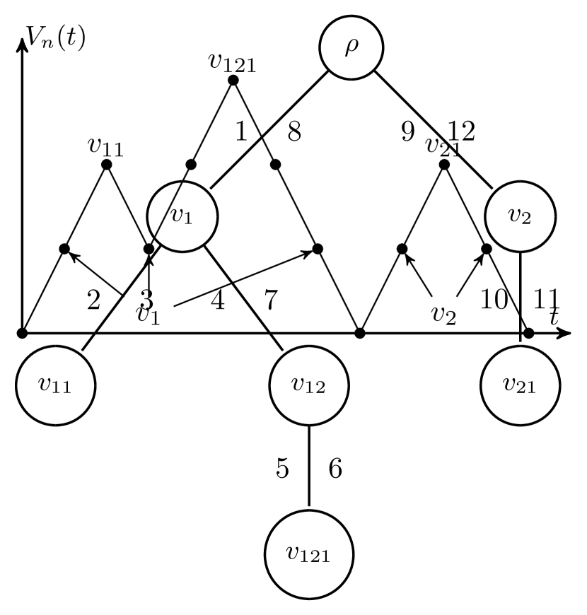
Figure 1: The depth-first walk $V_{n}(t)$ of a fixed tree.

Finally, define $R_{n}(i)\,{\buildrel{\mathrm{def}}\over{=}}\,\Phi_{f(i)}$ to be the value at the vertex visited after $i$ steps. For non-integer values $t$, $R_{n}(t)$ is defined by linearly interpolating the integer values. Also define $\widetilde{R}_{n}(t)$ by $\widetilde{R}_{n}(t)\,{\buildrel{\mathrm{def}}\over{=}}\,R_{n}(t)$ when $t\in\{0,1,\dots,2n\}$, and

$$\widetilde{R}_{n}(t)\,{\buildrel{\mathrm{def}}\over{=}}\,\left\{\begin{array}[]{lcl}R_{n}(\lfloor t\rfloor),&\text{if}&V_{n}(\lfloor t\rfloor)>V_{n}(\lceil t\rceil),\\ R_{n}(\lceil t\rceil),&\text{if}&V_{n}(\lfloor t\rfloor)<V_{n}(\lceil t\rceil).\end{array}\right.$$

In other words, $\widetilde{R}_{n}(t)$ takes the value of node $f(\lfloor t\rfloor)$ or $f(\lceil t\rceil)$, whichever is further from the root. We can recover $J(T_{n})$ from $\widetilde{R}_{n}(t)$ via

$$2J(T_{n})=\int_{0}^{2(n-1)}\widetilde{R}_{n}(t)dt.$$

Indeed, for each non-root node $v$ there are precisely two unit intervals during which $\widetilde{R}_{n}(t)$ draws its value from $v$, namely the two unit intervals during which the parent edge of $v$ is being traversed. Now, since $Q_{v}\sim\text{Unif}(-1/2,1/2)$ we have $|R_{n}(i)-R_{n}(i-1)|\leq 1/2$ for all $i>0$ and

$$\frac{J(T_{n})}{n^{5/4}}=\frac{1}{2n^{5/4}}\int_{0}^{2(n-1)}\widetilde{R}_{n}(t)\mathrm{d}t=\frac{1}{2n^{5/4}}\int_{0}^{2(n-1)}R_{n}(t)dt+O(n^{-1/4})=\int_{0}^{1}r_{n}(s)ds+o(1),$$

where $r_{n}(s)\,{\buildrel{\mathrm{def}}\over{=}}\,n^{-1/4}R_{n}(2(n-1)s)$. Also normalize $v_{n}(s)\,{\buildrel{\mathrm{def}}\over{=}}\,n^{-1/2}V_{n}(2(n-1)s)$. Theorem 2 of [36] (see also [26]) states that $(r_{n},v_{n})\overset{\mathrm{d}}{\longrightarrow}(r,v)$ in $C[0,1]\times C[0,1]$, with $r,v$ to be defined shortly.

Before defining $r$ and $v$, we will briefly motivate what they ought to be. Firstly, as the offspring distribution $\xi$ of $T_{n}$ satisfies $\mathbb{E}\left[\xi\right]=1$, we expect the tour $V_{n}$ to be roughly a random walk with zero-mean increments, conditioned to be non-negative and return to the origin at time $2(n-1)$, and the limiting law $v$ ought to be a Brownian excursion (up to a constant scale factor). Secondly, consider a node $u$ and the path $\rho=u_{0},u_{1}\dots,u_{d}=u$, where $d$ is the depth of $u$. We can define a random walk $\Phi_{u}(t)$ for $t=0,\dots,d$ by $\Phi_{u}(0)=0$ and $\Phi_{u}(t)=\sum_{i=1}^{t}Q_{u_{i}}$ for $t>0$, noting that $\Phi_{u}=\Phi_{u}(d)$. Under rescaling, the random walk $\Phi_{u}(t)$ will behave like Brownian motion. For any two nodes $u_{1},u_{2}$ with last common ancestor at depth $m$, the processes $\Phi_{u_{1}},\Phi_{u_{2}}$ agree for $t=0,\dots,m$, while any subsequent increments are independent. Hence $\text{Cov}(\Phi_{u_{1}},\Phi_{u_{2}})=cm$ for some constant $c>0$. Now, for any $i,j\in\{0,\dots,2(n-1)\}$, the nodes $f(i),f(j)$ at depths $V_{n}(i),V_{n}(j)$ have last common ancestor $f(k)$, where $k$ is such that $V_{n}(k)$ is minimal in the range $i\leq k\leq j$. Hence $r(s)$ should be normally distributed with variance given by $v(s)$, and the covariance of $r(s),r(t)$ proportional to $\min_{s\leq u\leq t}v(u)$.

We now define $r,v$ precisely. If ${\mathrm{Var}}\ \xi=\sigma^{2}$, then $v(s)\,{\buildrel{\mathrm{def}}\over{=}}\,2\sigma^{-1}e(s)$, where $e(s)$ is a standard Brownian excursion, as shown by Aldous [4, 5]. Conditioning on $v$, we define $r$ as a centered Gaussian process on $[0,1]$ with

$$\text{Cov}(r(s),r(t)\mid v)=\frac{1}{12}\min_{s\leq u\leq t}v(u)=\frac{1}{12\sigma}C(s,t),\qquad s\leq t.$$

The constant $1/12$ appears as the variance of the random increments $Q_{v}$. Again, Theorem 2 of [36] states that $(r_{n},v_{n})\overset{\mathrm{d}}{\longrightarrow}(r,v)$ in $C[0,1]^{2}$. We conclude that

$$\lim_{n\to\infty}\frac{J(T_{n})}{n^{5/4}}=\int_{0}^{1}r_{n}(t)dt+o(1)\overset{\mathrm{d}}{\longrightarrow}\int_{0}^{1}r(t)dt\,{\buildrel{\mathrm{def}}\over{=}}\,Y.$$

This integral is the object of study in [35], wherein it is shown that

$$Y\,{\buildrel{\mathrm{def}}\over{=}}\,\int_{0}^{1}r(t)dt\overset{\mathrm{d}}{=}\frac{1}{\sqrt{12\sigma}}\sqrt{\eta}\ {\cal N},$$

where ${\cal N}$ is a standard normal variable, $\eta$ is given by

$$\eta=\int_{[0,1]^{2}}C(s,t)\mathrm{d}s\ \mathrm{d}t,$$

and $\eta,{\cal N}$ are independent. The odd moments of $Y$ are zero, as this is the case for ${\cal N}$, and by [35, Theorem 1.1], for $k\geq 0$

$$\mathbb{E}\left[Y^{2k}\right]=\frac{1}{(12\sigma)^{k}}\frac{(2k!)\sqrt{\pi}}{2^{(9k-4)/2}\Gamma((5k-1)/2)}a_{k},$$

where $a_{1}=1$ and for $k\geq 2$,

$$a_{k}=2(5k-4)(5k-6)a_{k-1}+\sum_{i=1}^{k-1}a_{i}a_{k-i}.$$

In particular ([35, Theorem 1.2]),

$$\mathbb{E}\left[Y^{2k}\right]\sim\frac{1}{(12\sigma)^{k}}\frac{2\pi^{3/2}\beta}{5}(2k)^{1/2}(10e^{3})^{-2k/4}(2k)^{\frac{3}{4}\cdot 2k},$$

as $k\to\infty$, where $\beta=0.981038\dots$. Further analysis of the moments of $\eta$ and $Y$, including the moment generating function and tail estimates, can be found in [35].

Remark 5.1.

Conditioning on the value of $\eta$, the random variable $Y$ has variance $\eta/(12\sigma)$. The random variable $\eta$ can be seen as a scaled limit of the second common path length $\Upsilon_{2}(T_{n})$, which appeared in our earlier discussion on cumulants. Indeed, recall that $\Upsilon_{2}(T_{n})\,{\buildrel{\mathrm{def}}\over{=}}\,\sum_{u,v\in T_{n}}c(u,v)$, where $c(u,v)$ denotes the number of common ancestors of $u,v$.

5.1 Convergence of the moment generating function

The last bit of Theorem 1.16 which remains to be proved is that $\mathbb{E}\left[e^{tY_{n}}\right]\to\mathbb{E}\left[e^{tY}\right]$ for all fixed $t\in\mathbb{R}$. Since we have already shown $Y_{n}\overset{\mathrm{d}}{\longrightarrow}Y$, we can apply the Vitali convergence theorem once we have shown that the sequence $e^{tY_{n}}$ is uniformly integrable. This follows from the following lemma.

Lemma 5.2.

For all $n\in\mathbb{N}$ and $t\in\mathbb{R}$, there exist positive constants $C_{1}$ and $c_{1}$ which do not depend on $n$ such that

$$\mathbb{E}\left[e^{tY_{n}}\right]\leq C_{1}e^{c_{1}{t^{4}}}.$$

Proof.

Conditioned on $T_{n}$, we have by (1.8)

$$\mathbb{E}\left[e^{tY_{n}}\mid T_{n}\right]\leq\exp\left(\frac{1}{8}\Bigl{(}\frac{t}{n^{5/4}}\Bigr{)}^{2}\Upsilon_{2}(T_{n})\right)=\exp\left(\frac{t^{2}}{8}\cdot\frac{\Upsilon_{2}(T_{n})}{n^{5/2}}\right).$$

By (1.3), we have

$$\Upsilon_{2}(T_{n})=\sum_{u,v\in T_{n}}c(u,v)\leq n^{2}(H_{n}+1),$$

where $H_{n}$ denotes the height of $T_{n}$. It follows that

$$\mathbb{E}\left[e^{tY_{n}}\right]\leq\mathbb{E}\left[\exp\left(\frac{\Upsilon_{2}(T_{n})}{n^{5/2}}t^{2}\right)\right]\leq\mathbb{E}\left[\exp\left(\frac{H_{n}+1}{\sqrt{n}}t^{2}\right)\right]\leq e^{t^{2}}\mathbb{E}\left[\exp\left(\frac{H_{n}}{\sqrt{n}}t^{2}\right)\right].$$

The random variable $H_{n}$ has been well-studied. In particular, Addario-Berry et al. [1] showed that there exist positive constants $C_{2}$ and $c_{2}$ such that

$${\mathbb{P}\left\{H_{n}>x\right\}}\leq C_{2}\exp\left(-c_{2}\frac{x^{2}}{n}\right),$$

for all $n\in\mathbb{N}$ and $x\geq 0$. Therefore, we have

$$\mathbb{E}\left[\exp\left(\frac{H_{n}}{\sqrt{n}}t^{2}\right)\right]=1+\int_{0}^{\infty}e^{x}{\mathbb{P}\left\{\frac{H_{n}}{\sqrt{n}}t^{2}>x\right\}}\mathrm{d}x\leq 1+\int_{0}^{\infty}e^{x}C_{2}\exp\left(-c_{2}\frac{x^{2}}{t^{4}}\right)\mathrm{d}x\leq 1+C_{1}t^{2}e^{c_{3}{t^{4}}}$$

for some positive constants $c_{3}$ and $C_{1}$. (For the equality in the above computation, see [20, pp. 56].) Thus the lemma follows. ∎

References

- Addario-Berry et al. [2013] L. Addario-Berry, L. Devroye, and S. Janson. Sub-Gaussian tail bounds for the width and height of conditioned Galton-Watson trees. Ann. Probab., 41(2):1072–1087, 2013.
- Albert et al. [2018] M. Albert, C. Holmgren, T. Johansson, and F. Skerman. Permutations in Binary Trees and Split Trees. In 29th International Conference on Probabilistic, Combinatorial and Asymptotic Methods for the Analysis of Algorithms (AofA 2018), volume 110 of Leibniz International Proceedings in Informatics (LIPIcs), pages 9:1–9:12, Dagstuhl, Germany, 2018. Schloss Dagstuhl–Leibniz-Zentrum fuer Informatik.
- Aldous [1991a] D. Aldous. The continuum random tree. I. Ann. Probab., 19(1):1–28, 1991a.
- Aldous [1991b] D. Aldous. The continuum random tree. II. An overview. In Stochastic analysis (Durham, 1990), volume 167 of London Math. Soc. Lecture Note Ser., pages 23–70. Cambridge Univ. Press, Cambridge, 1991b.
- Aldous [1993] D. Aldous. The continuum random tree. III. Ann. Probab., 21(1):248–289, 1993.
- Baeza-Yates [1987] R. A. Baeza-Yates. Some average measures in -ary search trees. Inform. Process. Lett., 25(6):375–381, 1987.
- Bender [1973] E. A. Bender. Central and local limit theorems applied to asymptotic enumeration. J. Combinatorial Theory Ser. A, 15:91–111, 1973.
-
Bienaymé [1845]
I. J. Bienaymé.
De la loi de multiplication et de la durée des familles.
Société Philomatique Paris, 1845.
Reprinted in D. G. Kendall. The genealogy of genealogy branching processes before (and after) 1873. Bull. London Math. Soc., 7, 225–253, 1975. - Broutin and Holmgren [2012] N. Broutin and C. Holmgren. The total path length of split trees. Ann. Appl. Probab., 22(5):1745–1777, 2012.
- Cai and Devroye [2017] X. S. Cai and L. Devroye. A study of large fringe and non-fringe subtrees in conditional Galton-Watson trees. Latin American Journal of Probability and Mathematical Statistics, XIV:579–611, 2017.
- Chauvin and Pouyanne [2004] B. Chauvin and N. Pouyanne. -ary search trees when : a strong asymptotics for the space requirements. Random Structures Algorithms, 24(2):133–154, 2004.
- Coffman and Eve [1970] E. G. Coffman, Jr. and J. Eve. File structures using hashing functions. Commun. ACM, 13(7):427–432, July 1970.
- [13] K. Conrad. Probability distributions and maximum entropy. http://www.math.uconn.edu/~kconrad/blurbs/analysis/entropypost.pdf. Accessed: 2017-05-26.
- Cramer [1750] G. Cramer. Introduction à l’analyse des lignes courbes algébriques. 1750.
- Devroye [1993] L. Devroye. On the expected height of fringe-balanced trees. Acta Inform., 30(5):459–466, 1993.
- Devroye [1999] L. Devroye. Universal limit laws for depths in random trees. SIAM J. Comput., 28(2):409–432, 1999.
- Devroye et al. [2017] L. Devroye, C. Holmgren, and H. Sulzbach. The heavy path approach to Galton-Watson trees with an application to Apollonian networks. Preprint, Jan. 2017. arXiv:1701.02527
- [18] DLMF. NIST Digital Library of Mathematical Functions. http://dlmf.nist.gov/, Release 1.0.15 of 2017-06-01. F. W. J. Olver, A. B. Olde Daalhuis, D. W. Lozier, B. I. Schneider, R. F. Boisvert, C. W. Clark, B. R. Miller and B. V. Saunders, eds.
- Drmota et al. [2009] M. Drmota, A. Iksanov, M. Moehle, and U. Roesler. A limiting distribution for the number of cuts needed to isolate the root of a random recursive tree. Random Structures Algorithms, 34(3):319–336, 2009.
- Durrett [2010] R. Durrett. Probability: theory and examples, volume 31 of Cambridge Series in Statistical and Probabilistic Mathematics. Cambridge University Press, Cambridge, 4th edition, 2010. ISBN 978-0-521-76539-8.
- Feller [1968] W. Feller. An introduction to probability theory and its applications. Vol. I. John Wiley & Sons, Inc., New York-London-Sydney, 3rd edition, 1968.
- Finkel and Bentley [1974] R. A. Finkel and J. L. Bentley. Quad trees a data structure for retrieval on composite keys. Acta Informatica, 4(1):1–9, 1974.
- Flajolet et al. [1998] P. Flajolet, P. Poblete, and A. Viola. On the analysis of linear probing hashing. Algorithmica, 22(4):490–515, 1998.
- Flajolet et al. [2010] P. Flajolet, M. Roux, and B. Vallée. Digital trees and memoryless sources: from arithmetics to analysis. In 21st International Meeting on Probabilistic, Combinatorial, and Asymptotic Methods in the Analysis of Algorithms (AofA’10), Discrete Math. Theor. Comput. Sci. Proc., AM, pages 233–260. Assoc. Discrete Math. Theor. Comput. Sci., Nancy, 2010.
- Gessel et al. [1995] I. M. Gessel, B. E. Sagan, and Y. N. Yeh. Enumeration of trees by inversions. J. Graph Theory, 19(4):435–459, 1995.
- Gittenberger [2003] B. Gittenberger. A note on: “State spaces of the snake and its tour—convergence of the discrete snake”. J. Theoret. Probab., 16(4):1063–1067 (2004), 2003.
- Gut [2013] A. Gut. Probability: a graduate course. Springer Texts in Statistics. Springer, New York, 2nd edition, 2013.
- Hoare [1962] C. A. R. Hoare. Quicksort. Comput. J., 5:10–15, 1962.
- Hoeffding [1963] W. Hoeffding. Probability inequalities for sums of bounded random variables. J. Amer. Statist. Assoc., 58:13–30, 1963.
- Holmgren [2012] C. Holmgren. Novel characteristic of split trees by use of renewal theory. Electron. J. Probab., 17:no. 5, 27, 2012.
- Janson [2003] S. Janson. The Wiener index of simply generated random trees. Random Structures Algorithms, 22(4):337–358, 2003.
- Janson [2012] S. Janson. Simply generated trees, conditioned Galton-Watson trees, random allocations and condensation: extended abstract. In 23rd Intern. Meeting on Probabilistic, Combinatorial, and Asymptotic Methods for the Analysis of Algorithms (AofA’12), Discrete Math. Theor. Comput. Sci. Proc., AQ, pages 479–490. Assoc. Discrete Math. Theor. Comput. Sci., Nancy, 2012.
- Janson [2016] S. Janson. Asymptotic normality of fringe subtrees and additive functionals in conditioned Galton-Watson trees. Random Structures Algorithms, 48(1):57–101, 2016.
- Janson [2017] S. Janson. Random recursive trees and preferential attachment trees are random split trees. Preprint, June 2017. arXiv:1706.05487
- Janson and Chassaing [2004] S. Janson and P. Chassaing. The center of mass of the ISE and the Wiener index of trees. Electron. Comm. Probab., 9:178–187, 2004.
- Janson and Marckert [2005] S. Janson and J.-F. Marckert. Convergence of discrete snakes. J. Theoret. Probab., 18(3):615–647, 2005.
- Knuth [1998] D. E. Knuth. The art of computer programming. Vol. 3. Addison-Wesley, Reading, MA, 1998. ISBN 0-201-89685-0.
- Kortchemski [2017] I. Kortchemski. Sub-exponential tail bounds for conditioned stable Bienaymé-Galton-Watson trees. Probab. Theory Related Fields, 168(1-2):1–40, 2017.
- Louchard and Prodinger [2003] G. Louchard and H. Prodinger. The number of inversions in permutations: a saddle point approach. J. Integer Seq., 6(2):Article 03.2.8, 19, 2003.
- Mahmoud and Pittel [1989] H. M. Mahmoud and B. Pittel. Analysis of the space of search trees under the random insertion algorithm. J. Algorithms, 10(1):52–75, 1989.
- Mallows and Riordan [1968] C. L. Mallows and J. Riordan. The inversion enumerator for labeled trees. Bull. Amer. Math. Soc., 74:92–94, 1968.
- Margolius [2001] B. H. Margolius. Permutations with inversions. J. Integer Seq., 4(2):Article 01.2.4, 13, 2001.
- Neininger [2001] R. Neininger. On a multivariate contraction method for random recursive structures with applications to Quicksort. Random Structures Algorithms, 19(3-4):498–524, 2001.
- Neininger and Rüschendorf [1999] R. Neininger and L. Rüschendorf. On the internal path length of -dimensional quad trees. Random Structures Algorithms, 15(1):25–41, 1999.
- Neininger and Rüschendorf [2004] R. Neininger and L. Rüschendorf. A general limit theorem for recursive algorithms and combinatorial structures. Ann. Appl. Probab., 14(1):378–418, 2004.
- Panholzer and Seitz [2012] A. Panholzer and G. Seitz. Limiting distributions for the number of inversions in labelled tree families. Ann. Comb., 16(4):847–870, 2012.
- Pyke [1965] R. Pyke. Spacings. (With discussion.). J. Roy. Statist. Soc. Ser. B, 27:395–449, 1965.
- Régnier and Jacquet [1989] M. Régnier and P. Jacquet. New results on the size of tries. IEEE Trans. Inform. Theory, 35(1):203–205, 1989.
- Rösler [1991] U. Rösler. A limit theorem for “Quicksort”. RAIRO Inform. Théor. Appl., 25(1):85–100, 1991.
- Rösler [2001] U. Rösler. On the analysis of stochastic divide and conquer algorithms. Algorithmica, 29(1-2):238–261, 2001.
- Rösler and Rüschendorf [2001] U. Rösler and L. Rüschendorf. The contraction method for recursive algorithms. Algorithmica, 29(1-2):3–33, 2001.
- Sachkov [1997] V. N. Sachkov. Probabilistic methods in combinatorial analysis, volume 56 of Encyclopedia of Mathematics and its Applications. Cambridge University Press, Cambridge, 1997. ISBN 0-521-45512-X. Translated from the Russian, Revised by the author.
- Smith [1995] P. J. Smith. A recursive formulation of the old problem of obtaining moments from cumulants and vice versa. Amer. Statist., 49(2):217–218, 1995.
- Walker and Wood [1976] A. Walker and D. Wood. Locally balanced binary trees. The Computer Journal, 19(4):322–325, 1976.
- Watson and Galton [1875] H. W. Watson and F. Galton. On the probability of the extinction of families. The Journal of the Anthropological Institute of Great Britain and Ireland, 4:138–144, 1875.