Quantitative reconstructions in multi-modal photoacoustic and optical coherence tomography imaging

Abstract

In this paper we perform quantitative reconstruction of the electric susceptibility and the Grüneisen parameter of a non-magnetic linear dielectric medium using measurement of a multi-modal photoacoustic and optical coherence tomography system. We consider the mathematical model presented in [11], where a Fredholm integral equation of the first kind for the Grüneisen parameter was derived. For the numerical solution of the integral equation we consider a Galerkin type method.

¹Computational Science Center
University of Vienna
Oskar-Morgenstern-Platz 1
A-1090 Vienna, Austria

²Johann Radon Institute for Computational
 and Applied Mathematics (RICAM)
Altenbergerstraße 69
A-4040 Linz, Austria

1. Introduction

Tomographic imaging techniques visualize the inner structure of probes. Particularly relevant for this work are Optical Coherence Tomography (OCT) and Photoacoustic (PAT). In OCT a sample is placed in an interferometer and is illuminated by light pulses. Then, the backscattered light is measured far from the medium, see for instance [7, 9, 14]. PAT visualizes the capability of a medium to transform optical (infrared) waves into ultrasound waves to be measured on the surface of the medium [17, 28, 30]. PAT is called coupled physics imaging technique since it combines two kind of waves [1]. As stand alone imaging techniques PAT and OCT are not capable of recovering all diagnostically relevant physical parameters, but only some combinations of them, see [3] for PAT and [12] for OCT.

Recently setups which combine different imaging modalities, have been investigated mathematically with the objective to reconstruct more diagnostically relevant physical parameters from the measurements. Particular applications are coupled physics imaging systems and elastography [2, 20, 29], to name but a few. We refer to these techniques as hybrid imaging or multi-modal imaging systems. Note that in the mathematical literature the name hybrid imaging is also used for coupled physics imaging.

In this work we consider the multi-modal PAT/OCT system, developed for imaging biological tissues, see [10, 21, 22, 23, 31]. We show that with such a system, in contrast to the single modality setups, we obtain sufficient measurements which allow us to extract quantitative information on the electric susceptibility and the Grüneisen parameter of the sample. In the multi-modal PAT/OCT system, two different excitation laser systems, both operating in the same wavelength range, are used. The PAT and OCT scans are performed sequentially and vary a lot in acquisition times (around 5 minutes in PAT and less than 30 seconds in OCT). The obtained PAT and OCT images are co-registered afterwards.

In Section 2, we describe mathematically the multi-modal PAT/OCT setup. We use the model, from [11], based on Maxwell’s equations for the electric permittivity. In Section 3, we present the equivalence of the inverse problem of recovering both optical parameters with the solution of a Fredholm integral equation of the first kind for the Grüneisen parameter. Here the kernel of the integral operator depends on the PAT measurements.

We propose a numerical reconstruction method based on a Galerkin method using a series expansion of the unknown functions with respect to Hermite functions, see Section 4. The discretization of the continuous integral operator results in a system of linear algebraic equations. We solve the matrix equation using Tikhonov regularization. Numerical results which justify the feasibility of the proposed method are presented in Section 5.

2. The multi-modal PAT/OCT system

We consider the two modalities independently. Full field illumination is used in PAT and focused in OCT. The medium in OCT is illuminated by a Gaussian light. However, we can assume that the plane wave illumination is still valid [14].

2.1. Light propagation

We consider macroscopic Maxwell’s equations in order to model the interaction of the incoming light with the sample. These equations describe the time evolution of the electric and magnetic fields $E$ and $B$ for given charge density $\rho$ and electric current $J$:

$$\operatorname{div}_{x}D(t,x) =4\pi\rho(t,x),\quad t\in\mathbbm{R},\;x\in\mathbbm{R}^{3},$$ (1a)

$$\operatorname{div}_{x}B(t,x) =0,\quad t\in\mathbbm{R},\;x\in\mathbbm{R}^{3},$$ (1b)

$$\operatorname{curl}_{x}E(t,x) =-\frac{1}{c}\partial_{t}B(t,x),\quad t\in\mathbbm{R},\;x\in\mathbbm{R}^{3},$$ (1c)

$$\operatorname{curl}_{x}H(t,x) =\frac{1}{c}\partial_{t}D(t,x)+\frac{4\pi}{c}J(t,x),\quad t\in\mathbbm{R},\;x\in\mathbbm{R}^{3},$$ (1d)

where $D\equiv E+4\pi P$ is the electric displacement and $H\equiv B-4\pi M$ denotes the effective magnetic field, related to the electric and magnetic polarization fields $P$ and $M,$ respectively. We specify the material properties of the medium.

Definition .

The medium is called non-magnetic if $M=0$, and perfect linear dielectric and isotropic if there exist a scalar function $\chi\in C^{\infty}_{\mathrm{c}}(\mathbbm{R}\times\mathbbm{R}^{3};\mathbbm{R})$ the electric susceptibility, with $\chi(t,x)=0$ for all $t<0$, $x\in\mathbbm{R}^{3},$ (this property is referenced as causality), such that

$$P(t,x) =\int_{\mathbbm{R}}\chi(\tau,x)E(t-\tau,x)\,\mathrm{d}\tau,$$ (2a)

$$J(t,x) =0.$$ (2b)

The electric susceptibility describes the optical properties of the medium and is the parameter to be determined. In addition, we assume that the medium has no free charges, meaning $\rho=0$ in (1a).

Under the assumptions (2) of subsection 2.1, combining equations (1c) and (1d) we obtain the vector Helmholtz equation for the electric field

$$\operatorname{curl}_{x}\operatorname{curl}_{x}E(t,x)+\frac{1}{c^{2}}\partial_{tt}E(t,x)=-\frac{4\pi}{c^{2}}\int_{\mathbbm{R}}\partial_{tt}\chi(\tau,x)E(t-\tau,x)\,\mathrm{d}\tau.$$ (3)

Let $\Omega\subset\mathbbm{R}^{3}$ denote the domain where the object is located, meaning $\operatorname{supp}\chi(t,\cdot)\subset\Omega$ for all $t\in\mathbbm{R}.$

Definition .

We call $E^{(0)}$ an initial field if it satisfies the wave equation

$$\Delta_{x}E^{(0)}(t,x)-\frac{1}{c^{2}}\partial_{tt}E^{(0)}(t,x)=0,$$ (4)

and $\operatorname{div}_{x}E^{(0)}=0,$ and does not interact with the medium until the time $t=0,$ meaning

$$\operatorname{supp}E^{(0)}(t,\cdot)\cap\Omega=\emptyset\quad\text{for all}\quad t<0.$$

The initial pulse $E^{(0)}$ is a vacuum solution of Maxwell’s equations, meaning it satisfies (3) with $\chi\equiv 0.$ Indeed, using the vector identity $\operatorname{curl}_{x}\operatorname{curl}_{x}E=\mbox{grad}_{x}\operatorname{div}_{x}E-\Delta_{x}E$ in (3) we obtain the wave equation (4), since $\operatorname{div}_{x}E^{(0)}=0.$

Then, if the medium is given by subsection 2.1, we consider $E$ as the solution of (3) with initial condition

$$E(t,x)=E^{(0)}(t,x)\quad\text{for all}\quad t<0,\,x\in\mathbbm{R}^{3}.$$ (5)

2.1.1 Specific illumination

For both imaging modalities we consider the same incoming field. We use the convention

$$\hat{f}(\omega,x)=\int_{\mathbbm{R}}f(t,x)\mathrm{e}^{\mathrm{i}\omega t}\,\mathrm{d}t,$$

for the Fourier transform of a integrable function $f$ with respect to time $t.$

The multiple laser pulses centered around different frequencies $\nu$, are described by the initial electric fields

$$E^{(0)}_{\nu}(t,x)=f_{\nu}(t+\tfrac{x_{3}}{c})\eta,\quad\nu>0,$$ (6)

which describe linearly polarized plane waves moving in the direction $-e_{3},$ for some $f_{\nu}\in C^{\infty}_{\mathrm{c}}(\mathbbm{R})$ and fixed polarization vector $\eta\in\mathbbm{R}^{2}\times\{0\},$ with $|\eta|=1.$ These fields satisfy (4) for every $\nu$. We assume that the Fourier transform of $f_{\nu}$ satisfies

$$\operatorname{supp}\hat{f}_{\nu}\subset[-\nu-\varepsilon,-\nu+\varepsilon]\cup[\nu-\varepsilon,\nu+\varepsilon],$$ (7)

for some sufficiently small $\varepsilon>0$. We denote by $E_{\nu}$ the solution of (3) for the specific initial field $E^{(0)}_{\nu}.$ The multiple illuminations result to multi-frequency PAT measurements, but they do not provide extra information in OCT, see [11, Lemma 3.6].

2.2. PAT measurements

Let the medium be defined as in Definition 2.1. Then, we estimate the averaged change in energy density around a point $x,$ for every $\nu,$ by

$$\partial_{t}\mathcal{E}_{\nu}(t,x)\approx\left<E_{\nu}(t,x),\partial_{t}P_{\nu}(t,x)\right>.$$ (8)

In order to derive the above formula we have to consider the interaction of the medium with the incoming electromagnetic wave locally. For a derivation, using microscopic Maxwell’s equations, see for instance [11, Section 4].

The laser pulse is absorbed by the medium and part of it is transformed into heat. This generates a pressure wave which is then measured on the object surface. Since the laser pulse is typically very short, the propagation of the acoustic wave during thermal absorption can be neglected. Then, we consider as PAT measurements the initial pressure density $p$ which is proportional to the absorbed energy

$$p_{\nu}(x)=\Gamma(x)\int_{\mathbbm{R}}\partial_{t}\mathcal{E}_{\nu}(\tau,x)\,\mathrm{d}\tau.$$ (9)

The proportionality factor $\Gamma$ is the Grüneisen parameter, a parameter which, together with the susceptibility $\chi,$ describes the optical properties of our medium.

2.3. OCT measurements

In the frequency domain, the equation (3) and the condition (5) result to an integral equation of Lippmann-Schwinger type [8, 12].

Lemma 2.1.

Let the medium be defined as in subsection 2.1 and $E_{\nu}^{(0)}$ as in subsection 2.1. If $E_{\nu}$ is a solution of (3) with initial values (5), then its Fourier transform solves the Lippmann-Schwinger integral equation

$$\hat{E}_{\nu}(\omega,x)=\hat{E}_{\nu}^{(0)}(\omega,x)+\left(\frac{\omega^{2}}{c^{2}}+\operatorname{grad}_{x}\operatorname{div}_{x}\right)\int_{\mathbbm{R}^{3}}\frac{\mathrm{e}^{\mathrm{i}\frac{\omega}{c}|x-y|}}{|x-y|}\hat{\chi}(\omega,y)\hat{E}_{\nu}(\omega,y)\,\mathrm{d}y.$$ (10)

Due to the limiting penetration depth of OCT (1 to 2 millimeters), the medium can be considered as weakly scattering, since only single scattering events will be measured. In addition, in OCT the measurements are performed in a distance much larger compared to the size of the medium.

The Born approximation allows us to obtain an explicit form for $\hat{E}_{\nu}$ from the Lippmann-Schwinger equation (10). In the limiting case $\hat{\chi}\rightarrow 0,$ we take the first order approximation of the electric field by replacing $\hat{E}_{\nu}$ with $\hat{E}_{\nu}^{(0)}$ in the integrand of (10).

We write $x$ in spherical coordinates $x=\rho\vartheta,\,\rho>0,\,\vartheta\in S^{2}.$ Under the far-field approximation, we consider the asymptotic behavior of the expression (10) for $\rho\rightarrow\infty,$ uniformly in $\vartheta$

$$\hat{E}_{\nu}(\omega,\rho\vartheta)\simeq\hat{E}_{\nu}^{(0)}(\omega,\rho\vartheta)-\mathrm{e}^{\mathrm{i}\frac{\omega}{c}\rho}\frac{\omega^{2}}{\rho c^{2}}\int_{\mathbbm{R}^{3}}\vartheta\times\big{(}\vartheta\times(\hat{\chi}(\omega,y)\hat{E}_{\nu}(\omega,y))\big{)}\mathrm{e}^{-\mathrm{i}\frac{\omega}{c}\left<\vartheta,y\right>}\,\mathrm{d}y.$$

Then, we define

$$\hat{E}_{\nu}^{(1)}(\omega,\rho\vartheta):=\hat{E}_{\nu}^{(0)}(\omega,\rho\vartheta)-\mathrm{e}^{\mathrm{i}\frac{\omega}{c}\rho}\frac{\omega^{2}}{\rho c^{2}}\int_{\mathbbm{R}^{3}}\vartheta\times\big{(}\vartheta\times(\hat{\chi}(\omega,y)\hat{E}_{\nu}^{(0)}(\omega,y))\big{)}\mathrm{e}^{-\mathrm{i}\frac{\omega}{c}\left<\vartheta,y\right>}\,\mathrm{d}y,$$ (11)

as the electric field considering both approximations.

The approximated backscattered light $\hat{E}_{\nu}^{(1)}-\hat{E}_{\nu}^{(0)}$ is combined with a known back-reflected field and its correlation is measured at each point on the detector surface. Under some assumptions on the incident illumination we state that what we actually measure in OCT is the backscattered light at a detector placed far from the medium [12, Proposition 8].

Then, we formulate the direct problem as:

Definition (direct problem).

Given a medium as in subsection 2.1 with susceptibility $\chi$ and Grüneisen parameter $\Gamma,$ and incident illumination $E_{\nu}^{(0)}$ of the form (6), the direct problem is to find the PAT measurements $p_{\nu}(x),\,x\in\Omega,\,\nu>0,$ given by (9), and the OCT measurements

$$(\hat{E}_{\nu}^{(1)}-\hat{E}_{\nu}^{(0)})(\omega,\rho\vartheta),\,\omega\in\mathbbm{R}\setminus\{0\},\,\vartheta\in S^{2}_{+}=\{\vartheta\in S^{2}\mid\vartheta_{3}>0\},\,\nu>0,$$

given by (11).

3. The Inverse Problem

In the following the assumptions on the medium (subsection 2.1) hold and especially the causality of $\chi.$ We denote by $\tilde{\chi}$ the three-dimensional Fourier transform of $\hat{\chi}$ with respect to space

$$\tilde{\chi}(\omega,k)=\int_{\mathbbm{R}^{3}}\hat{\chi}(\omega,x)\mathrm{e}^{-\mathrm{i}\langle k,x\rangle}\,\mathrm{d}x.$$

The OCT system, by replacing $E_{\nu}^{(0)}$ in (11) and simple calculations, see [12, Proposition 9], provide us with the data

$$\tilde{\chi}(\omega,\tfrac{\omega}{c}(\vartheta+e_{3})),\quad\omega\in\mathbbm{R}\setminus\{0\},\;\vartheta\in S^{2}_{+}.$$ (12)

However, in practice, these data are incomplete because of the band-limited source and size of the detector. Thus, we get the spatial and temporal Fourier transform of $\chi$ only in a subset of $\mathbbm{R}\times\mathbbm{R}^{3}.$

Then, the inverse problem we address here reads:

Definition (inverse problem).

Given a medium as in subsection 2.1 and incident fields $E^{(0)}_{\nu}$ of the form (6) for all $\nu>0,$ the inverse problem is to recover the parameters $\hat{\chi}$ and $\Gamma$ given the internal PAT measurements $p_{\nu}(x),$ for $x\in\Omega,$ and all $\nu>0,$ given by (9), and the external OCT data $\tilde{\chi}(\omega,\tfrac{\omega}{c}(\vartheta+e_{3})),\,\omega\in\mathbbm{R}\setminus\{0\},\,\vartheta\in S^{2}_{+},$ given by (12).

Similar inverse problems have been considered in [4, 6] where the far-field measurements from OCT are replaced by boundary measurements and in [5] for the diffusion approximation of the radiative transfer equation.

To present an equivalent formulation of the inverse problem, we assume that in both imaging techniques, we illuminate with multiple laser pulses with small spectrum centered around different frequencies. This setup describes swept-source OCT and multi-frequency PAT measurements.

First we describe the PAT measurements for multiple laser pulses. We combine (8) and (9) to get

$$p_{\nu}(x)=\Gamma(x)\int_{\mathbbm{R}}\left<E_{\nu}(t,x),\partial_{t}P_{\nu}(t,x)\right>\,\mathrm{d}t,$$

where $E_{\nu}$ is the electric field generated by the laser pulse $E^{(0)}_{\nu}.$ Using the Fourier transform of (2a) we derive

$$p_{\nu}(x)=\Gamma(x)\frac{1}{2\pi}\int_{\mathbbm{R}}-\mathrm{i}\omega\hat{\chi}(\omega,x)|\hat{E}_{\nu}(\omega,x)|^{2}\,\mathrm{d}\omega.$$

Remark :

In the case of nonlinear medium, the polarization field $P$ is usually expressed as a power series of the electric field $E.$ Then, the third order term contributes to the so-called two-photon absorbed energy [15]. We refer to [27] for reconstructions in two-photon PAT.

As in OCT, we replace $E_{\nu}$ by the initial pulse $E_{\nu}^{(0)}$ and we approximate the PAT data by

$$p_{\nu}(x)\approx\Gamma(x)\frac{1}{2\pi}\int_{\mathbbm{R}}-\mathrm{i}\omega\hat{\chi}(\omega,x)|\hat{f}_{\nu}(\omega)|^{2}\,\mathrm{d}\omega,$$

since $|\eta|=1.$ The support of $\hat{f}_{\nu}$ is localized around the frequency $\nu$, see (7). Thus, we get in the limit $\varepsilon\to 0$ (for constant norm $\|\hat{f}_{\nu}\|_{2}$) that

$$p_{\nu}(x)\simeq\frac{1}{2\pi}\|\hat{f}_{\nu}\|_{2}^{2}\Gamma(x)(-\mathrm{i}\nu\hat{\chi}(\nu,x)+\mathrm{i}\nu\hat{\chi}(-\nu,x))=\frac{1}{\pi}\|\hat{f}_{\nu}\|_{2}^{2}\Gamma(x)\nu\operatorname{\Im m}(\hat{\chi}(\nu,x)).$$

We define $p(\nu,x):=\frac{\pi}{\nu}\|\hat{f}_{\nu}\|_{2}^{-2}\,p_{\nu}(x).$ Then, we get asymptotically

$$\boxed{p(\nu,x)\simeq\Gamma(x)\operatorname{\Im m}(\hat{\chi}(\nu,x)).}$$ (13)

We assume measurements for all frequencies $\nu>0.$ Recall that $\chi$ is a causal real valued function. Then the real part of $\hat{\chi}$ can be completely determined from the imaginary part via the Kramers–Kronig relation

$$\operatorname{\Re e}(\hat{\chi}(\omega,x))=\mathcal{H}[\operatorname{\Im m}\hat{\chi}](\omega,x).$$

Here, $\mathcal{H}$ denotes the Hilbert transform with respect to frequency

$$\mathcal{H}[f](\omega,x)=\frac{1}{\pi}\int_{\mathbbm{R}}\frac{f(\tilde{\omega},x)}{\tilde{\omega}-\omega}\,\mathrm{d}\tilde{\omega}.$$

We use the above two equations in order to describe the OCT data (12). Then we end up with the Fredholm integral equation

$$\boxed{\int_{\mathbbm{R}^{3}}\left(\mathcal{H}[p](\omega,y)+\mathrm{i}p(\omega,y)\right)\,\mathrm{e}^{-\mathrm{i}\tfrac{\omega}{c}\langle\vartheta+e_{3},y\rangle}\frac{1}{\Gamma(y)}\,\mathrm{d}y=\tilde{\chi}(\omega,\tfrac{\omega}{c}(\vartheta+e_{3})),}$$ (14)

for the Grüneisen parameter $\Gamma.$ Once (14) is solved, we can easily recover the imaginary part of $\hat{\chi}$ from equation (13).

Remark :

If the medium is a perturbation of a single material then the above equation is transformed to a Fredholm integral equation of the second kind for a new function depending on $\tfrac{1}{\Gamma}$ [11]. At least in this simplified setting, we find that using the multi-modal model PAT/OCT we can (uniquely) determine the Grüneisen parameter and the susceptibility $\chi$ describing the absorption and scattering properties of the medium.

Observing the formulas (13) and (14), we rewrite the inverse problem (Section 3) in its simplified form:

Definition (simplified inverse problem).

Find $\Gamma(x)$ and $\hat{\chi}(\omega,x),$ given $\tilde{\chi}(\omega,\tfrac{\omega}{c}(\vartheta+e_{3})),$ for all $\omega\in\mathbbm{R}\setminus\{0\},\;\vartheta\in S^{2}_{+}$ (approximated OCT data) and the product $\Gamma(x)\operatorname{\Im m}(\hat{\chi}(\omega,x)),$ for all $\omega\in\mathbbm{R}\setminus\{0\},\;x\in\Omega$ (approximated PAT data).

In the following section we present a Galerkin type method for the numerical solution of equation (14) considering two types of media. There exist also other projection methods for the numerical solution of integral equations, the collocation method and the method of moments and quadrature methods, like the Nyström method [16, 19, 25].

4. Numerical Implementation

Without loss of generality we set $c=1$ and we specify $\Omega=[-l,l]^{3}.$ For the numerical examples we have to introduce the parameter $\tilde{\Gamma},$ related to the physical parameter $\Gamma,$ which satisfies

$$\tilde{\Gamma}(x)=\frac{1}{\Gamma(x)},\quad\mbox{for }x\in\Omega,\quad\mbox{and}\quad\operatorname{supp}\tilde{\Gamma}\subset\Omega_{L},$$

where $\Omega_{L}=[-L,L]^{3},$ for $L>l.$ This is possible since $\Gamma\geq\Gamma_{0}>0,$ with $\Gamma_{0}\sim 1$ in biological tissues. In addition, we do not consider the restrictions on the frequency in the following analysis.

4.1. Medium with depth-dependent coefficients

In the first example, we assume that both parameters $\Gamma$ and $\hat{\chi}$ are only depth-dependent, meaning that they vary only in the incident direction. Then, $\tilde{\Gamma}$ and $\hat{\chi}$ admit the forms

$$\tilde{\Gamma}(x)=\mathbbm{1}_{[-L,L]^{2}}(x_{1},x_{2})\gamma(x_{3}),\quad\text{and}\quad\hat{\chi}(\omega,x)=\mathbbm{1}_{[-l,l]^{2}}(x_{1},x_{2})\psi(\omega,x_{3}),$$

respectively. Here $\mathbbm{1}$ denotes the characteristic function. This case represents media which have a multilayer structure with depth-dependent properties, like the human skin. If the illumination is focused to a small region inside the object and this region is small enough such that the functions can be assumed constant in both directions $e_{1}$ and $e_{2},$ we get the above forms.

Thus the problem reduces to the problem of recovering a one-dimensional function $\gamma$. We do not consider the two-dimensional detector array but only the measurements at the single point detector located at the position $(0,\,0,\,d),$ meaning we set $\vartheta=e_{3}.$ Then, the equation (14) takes the simplified form

$$\int_{\mathbbm{R}}\left(\mathcal{H}[p](\omega,y_{3})+\mathrm{i}p(\omega,y_{3})\right)\mathrm{e}^{-\mathrm{i}2\omega y_{3}}\gamma(y_{3})\,\mathrm{d}y_{3}=m(\omega),$$ (15)

where $m(\omega):=(\tfrac{\pi}{l})^{2}\tilde{\chi}(\omega,2\omega e_{3}).$

Let $p\in(L^{2}(\mathbbm{R}))^{2}$ and $\gamma\in L^{2}(\mathbbm{R}).$ Since the kernel of the integral operator and the right-hand side in (15) have specific structures containing Hilbert and Fourier transforms we consider as orthonormal basis of $L^{2}(\mathbbm{R})$ the Hermite functions $h_{k},\,k\in\mathbbm{N}_{0}$. In addition the multi-dimensional Hermite functions can be written as sum of products of the usual Hermite functions. Their properties are given in Appendix. Other choices are also possible, especially when we treat the three-dimensional problem with real data, for instant using wavelets as basis functions.

Let $x\in\mathbbm{R}.$ The Hermite polynomials are defined by the formula

$$H_{k}(x)=(-1)^{k}\frac{d^{k}}{dx^{k}}(\mathrm{e}^{-x^{2}})\mathrm{e}^{x^{2}},\quad k\in\mathbbm{N}_{0}.$$

The normalized Hermite functions are given by

$$h_{k}(x)=\alpha_{k}H_{k}(x)\mathrm{e}^{-\tfrac{1}{2}x^{2}},k\in\mathbbm{N}_{0},$$ (16)

where $\alpha_{k}=(2^{k}k!\sqrt{\pi})^{-\tfrac{1}{2}}.$ The functions $h_{k}$ satisfy the orthonormality condition

$$\int_{\mathbbm{R}}h_{k}(x)h_{l}(x)\,\mathrm{d}x=\delta_{k,l}.$$

Proposition .

Let $x\in\mathbbm{R}.$ We consider the expansion

$$\gamma(\tfrac{x}{2})=\sum_{k=0}^{\infty}\gamma_{k}h_{k}(x),$$ (17)

with coefficients $\gamma_{k}\in\mathbbm{R},\,k\in\mathbbm{N}_{0}$ and

$$p(\omega,\tfrac{x}{2})=\sum_{k,l=0}^{\infty}p_{k,l}h_{k}(\omega)h_{l}(x),$$ (18)

with coefficients $p_{k,l}\in\mathbbm{R},\,k,l\in\mathbbm{N}_{0}.$ Then, if $\gamma$ satisfies the integral equation (15), the coefficients $\gamma_{k},\,k\in\mathbbm{N}_{0}$ solve the equation

$$\sum_{j=0}^{\infty}\gamma_{j}A_{j,s}=m_{s},\quad s\in\mathbbm{N}_{0},$$ (19)

where

$$m_{s} =\int_{\mathbbm{R}}2\mathrm{e}^{\tfrac{\omega^{2}}{4}}m(\omega)h_{s}(\omega)\,\mathrm{d}\omega,$$

$$A_{j,s} :=\sum_{k,l=0}^{\infty}(\tilde{p}_{k,l}+\mathrm{i}p_{k,l})\sum_{n=0}^{\min(j,l)}\beta_{j,l,n}\,\zeta_{j+l-2n}\frac{(j+l-2n)!}{2^{j+l-2n}}\sum_{r=0}^{\left[\tfrac{j+l-2n}{2}\right]}\frac{1}{r!q!\,\alpha_{q}}$$

$$\phantom{=}\times\sum_{s=0}^{\infty}\mathbbm{1}_{[|k-q|,k+q]}(s)\beta_{k,q,\tfrac{k+q-s}{2}},\quad\mbox{and }q:=j+l-2n-2r.$$

Before proving this Proposition, we state the following lemma. Its proof is presented in Appendix.

Lemma 4.1.

Let $k\in\mathbbm{N}_{0}.$ Then

$$\int_{\mathbbm{R}}\mathrm{e}^{-\tfrac{x^{2}}{2}}h_{k}(x)\mathrm{e}^{-\mathrm{i}\omega x}\,\mathrm{d}x=\zeta_{k}\mathrm{e}^{-\tfrac{\omega^{2}}{4}}\omega^{k},$$ (20)

where $\zeta_{k}=2\sqrt{\pi^{3}}(-\mathrm{i})^{k}\alpha_{k},$ for $\alpha_{k}$ as in (16).

Proof (subsection 4.1):

Using the expansion (18) and considering (44), we get

$$\mathcal{H}[p](\omega,x)+\mathrm{i}p(\omega,x)=\sum_{k,l=0}^{\infty}(\tilde{p}_{k,l}+\mathrm{i}p_{k,l})h_{k}(\omega)h_{l}(2x).$$

The coefficients $\tilde{p}_{k,l},$ using (45), are given by

$$\tilde{p}_{k,l}=(-\mathrm{i})^{k+1}\sum_{m=0}^{\infty}p_{m,l}(-\mathrm{i})^{m}\int_{\mathbbm{R}}\operatorname{sign}(\omega)h_{k}(\omega)h_{m}(\omega)\,\mathrm{d}\omega.$$

We substitute the above expansions and (17) in (15) and we obtain

$$\sum_{j=0}^{\infty}\gamma_{j}\sum_{k,l=0}^{\infty}(\tilde{p}_{k,l}+\mathrm{i}p_{k,l})h_{k}(\omega)\int_{\mathbbm{R}}h_{j}(2y_{3})h_{l}(2y_{3})\mathrm{e}^{-\mathrm{i}2\omega y_{3}}\,\mathrm{d}y_{3}=m(\omega).$$

We rewrite the product of the two Hermite functions in the integrand using the formula (41) and we change variables to get

$$\sum_{j=0}^{\infty}\gamma_{j}\sum_{k,l=0}^{\infty}(\tilde{p}_{k,l}+\mathrm{i}p_{k,l})h_{k}(\omega)\sum_{n=0}^{\min(j,l)}\beta_{j,l,n}\int_{\mathbbm{R}}\mathrm{e}^{-\tfrac{x^{2}}{2}}h_{j+l-2n}(x)\mathrm{e}^{-\mathrm{i}\omega x}\,\mathrm{d}x=2m(\omega).$$ (21)

Then, equation (21) using (20) takes the form

$$\sum_{j=0}^{\infty}\gamma_{j}\sum_{k,l=0}^{\infty}(\tilde{p}_{k,l}+\mathrm{i}p_{k,l})h_{k}(\omega)\sum_{n=0}^{\min(j,l)}\beta_{j,l,n}\,\zeta_{j+l-2n}\omega^{j+l-2n}=\tilde{m}(\omega),$$ (22)

where $\tilde{m}(\omega)=2\mathrm{e}^{\tfrac{\omega^{2}}{4}}m(\omega).$

Using (16) and (43), we get

$$\omega^{k}=\frac{k!}{2^{k}}\mathrm{e}^{\tfrac{\omega^{2}}{2}}\sum_{q=0}^{\left[\tfrac{k}{2}\right]}\frac{1}{q!(k-2q)!\alpha_{k-2q}}h_{k-2q}(\omega).$$ (23)

We substitute this expansion in (22) to obtain

$$\sum_{j=0}^{\infty}\gamma_{j}\sum_{k,l=0}^{\infty}(\tilde{p}_{k,l}+\mathrm{i}p_{k,l})\sum_{n=0}^{\min(j,l)}\beta_{j,l,n}\,\zeta_{j+l-2n}\frac{(j+l-2n)!}{2^{j+l-2n}}\mathrm{e}^{\tfrac{\omega^{2}}{2}}\\ \times\sum_{r=0}^{\left[\tfrac{j+l-2n}{2}\right]}\frac{1}{r!q!\alpha_{q}}h_{k}(\omega)h_{q}(\omega)=\tilde{m}(\omega),$$ (24)

where for simplicity we set $q:=j+l-2n-2r.$ Again the last product using (41) admits the form

$$h_{k}(\omega)h_{q}(\omega)=\mathrm{e}^{-\tfrac{\omega^{2}}{2}}\sum_{u=0}^{\min(k,q)}\beta_{k,q,u}h_{k+q-2u}(\omega).$$

We expand also the data using the same basis functions

$$\tilde{m}(\omega)=\sum_{k=0}^{\infty}m_{k}h_{k}(\omega),\quad\text{for}\quad m_{k}=\int_{\mathbbm{R}}\tilde{m}(\omega)h_{k}(\omega)\,\mathrm{d}\omega,$$

and in order to obtain a linear equation for $\gamma_{j}$ we have to enlarge the index of the last sum. We set $s:=k+q-2u$ and for $\tfrac{k+q-s}{2}\in\mathbbm{N}_{0}$ we reformulate (24) using the above formulas as

$$\sum_{j=0}^{\infty}\gamma_{j}\sum_{k,l=0}^{\infty}(\tilde{p}_{k,l}+\mathrm{i}p_{k,l})\sum_{n=0}^{\min(j,l)}\beta_{j,l,n}\,\zeta_{j+l-2n}\frac{(j+l-2n)!}{2^{j+l-2n}}\sum_{r=0}^{\left[\tfrac{j+l-2n}{2}\right]}\frac{1}{r!q!\,\alpha_{q}}\\ \times\sum_{s=0}^{\infty}\mathbbm{1}_{[|k-q|,k+q]}(s)\beta_{k,q,\tfrac{k+q-s}{2}}h_{s}(\omega)=\sum_{s=0}^{\infty}m_{s}h_{s}(\omega).$$

Equating the coefficients in the above equation yields (19).

The final step, for the Galerkin method, is to consider a finite dimensional subset of $L^{2}(\mathbbm{R}),$ meaning restrict ourselves to a finite number of coefficients. Let $j,k,l=0,...,N-1.$ Then the definitions used in the above analysis gives $q=0,...,2(N-1)$ and $s=0,...,3(N-1).$ Finally, the discrete linear system of (19) reads

$$\bm{A}\bm{\gamma}=\bm{m},$$ (25)

where $\bm{A}=(A_{s,j})\in\mathbbm{C}^{(3N-2)\times N},\bm{\gamma}=(\gamma_{j})\in\mathbbm{R}^{N}$ and $\bm{m}=(m_{s})\in\mathbbm{C}^{3N-2}.$

4.2. Medium with coefficients constant in one direction

In this case, we assume that both parameters are constant only in one direction, let us say in $e_{1}.$ Then, $\tilde{\Gamma}$ and $\hat{\chi}$ take the forms

$$\tilde{\Gamma}(x)=\mathbbm{1}_{[-L,L]}(x_{1})\gamma(x_{2},x_{3}),\quad\text{and}\quad\hat{\chi}(\omega,x)=\mathbbm{1}_{[-l,l]}(x_{1})\psi(\omega,x_{2},x_{3}),$$

respectively. This assumption results to a two-dimensional function $\gamma,$ a case more involved compared to subsection 4.1 that approximates better the unconditional general problem. Here, we need two-dimensional data, thus we have to consider measurements for all frequencies in a one-dimensional array, modeling measurement points on a line.

The equation (14), for $c=1,$ now takes the form

$$\int_{\mathbbm{R}}\int_{\mathbbm{R}}\left(\mathcal{H}[p](\omega,y_{2},y_{3})+\mathrm{i}p(\omega,y_{2},y_{3})\right)\mathrm{e}^{-\mathrm{i}\omega(\vartheta_{2}y_{2}+\tilde{\vartheta}_{3}y_{3})}\gamma(y_{2},y_{3})\,\mathrm{d}y_{2}\,\mathrm{d}y_{3}=m(\omega,\vartheta),$$ (26)

where $\tilde{\vartheta}_{3}=\vartheta_{3}+1,$ and $m(\omega,\vartheta):=\frac{\pi}{l}\tilde{\chi}(\omega,\tfrac{\omega}{c}(\vartheta+e_{3})).$

Proposition .

Let $x=(x_{1},x_{2})\in\mathbbm{R}^{2}.$ We use (46), for $\bm{k}=(k,\,l)$, and we expand $\gamma$ as

$$\gamma(x)=\sum_{\bm{k}=0}^{\infty}\gamma_{\bm{k}}h_{\bm{k}}(x)=\sum_{k,l=0}^{\infty}\gamma_{k,l}h_{k}(x_{1})h_{l}(x_{2}),$$ (27)

where the coefficients $\gamma_{k,l}$ are defined by

$$\gamma_{k,l}=\int_{\mathbbm{R}}\int_{\mathbbm{R}}\gamma(x_{1},x_{2})h_{k}(x_{1})h_{l}(x_{2})\,\mathrm{d}x_{1}\,\mathrm{d}x_{2},\quad k,l\in\mathbbm{N}_{0}.$$

and we assume the expansion

$$p(\omega,x)=\sum_{k,l,a=0}^{\infty}p_{k,l,a}h_{k}(\omega)h_{l}(x_{1})h_{a}(x_{2}),$$ (28)

where

$$p_{k,l,a}=\int_{\mathbbm{R}}\int_{\mathbbm{R}}\int_{\mathbbm{R}}p(\omega,x_{1},x_{2})h_{k}(\omega)h_{l}(x_{1})h_{a}(x_{2})\,\mathrm{d}\omega\,\mathrm{d}x_{1}\,\mathrm{d}x_{2},\quad k,l,a\in\mathbbm{N}_{0}$$

Then, if $\gamma$ solves the integral equation (26), its coefficients $\gamma_{k,l},\,k,l\in N_{0}$ satisfy the equation

$$\sum_{k,l=0}^{\infty}\gamma_{k,l}B_{k,l,\mu}(\vartheta)=m_{\mu}(\vartheta),\quad\mu\in\mathbbm{N}_{0},$$ (29)

for

$$m_{\mu}(\vartheta) =\int_{\mathbbm{R}}\mathrm{e}^{\frac{\omega^{2}\tilde{\vartheta}_{3}}{2}}m(\vartheta,\omega)h_{\mu}(\omega)\,\mathrm{d}\omega,$$

$$B_{k,l,\mu}(\vartheta) =\sum_{a,n,u=0}^{\infty}(\tilde{p}_{a,n,u}+\mathrm{i}p_{a,n,u})\sum_{r=0}^{\min(k,n)}\beta_{k,n,r}\,\zeta_{k+n-2r}\vartheta_{2}^{k+n-2r}$$

$$\phantom{=}\times\sum_{q=0}^{\min(l,u)}\beta_{l,u,q}\,\zeta_{l+u-2q}\tilde{\vartheta}_{3}^{l+u-2q}\frac{s!}{2^{s}}\sum_{j=0}^{\left[\frac{s}{2}\right]}\frac{1}{j!(s-2j)!\alpha_{s-2j}}$$

$$\phantom{=}\times\mathbbm{1}_{[|a-s+2j|,a+s-2j]}(\mu)\beta_{a,s-2j,\frac{a+s-2j-\mu}{2}}\,,$$

with $s:=k+n+l+u-2r-2q.$

Proof:

The equation (26) using the expansions (27) and (28) results to

$$\sum_{k,l=0}^{\infty}\gamma_{k,l}\sum_{a,n,u=0}^{\infty}(\tilde{p}_{a,n,u}+\mathrm{i}p_{a,n,u})h_{a}(\omega)\int_{\mathbbm{R}}\int_{\mathbbm{R}}h_{k}(y_{2})h_{l}(y_{3})h_{n}(y_{2})\\ \times h_{u}(y_{3})\mathrm{e}^{-\mathrm{i}\omega(\vartheta_{2}y_{2}+\tilde{\vartheta}_{3}y_{3})}\,\mathrm{d}y_{2}\,\mathrm{d}y_{3}=m(\omega,\vartheta).$$

We apply twice the formula (41) for the product of two Hermite functions, to obtain

$$\sum_{k,l=0}^{\infty}\gamma_{k,l}\sum_{a,n,u=0}^{\infty}(\tilde{p}_{a,n,u}+\mathrm{i}p_{a,n,u})h_{a}(\omega)\sum_{r=0}^{\min(k,n)}\beta_{k,n,r}\int_{\mathbbm{R}}\mathrm{e}^{-\frac{y_{2}^{2}}{2}}h_{k+n-2r}(y_{2})\mathrm{e}^{-\mathrm{i}\omega\vartheta_{2}y_{2}}\,\mathrm{d}y_{2}\\ \times\sum_{q=0}^{\min(l,u)}\beta_{l,u,q}\int_{\mathbbm{R}}\mathrm{e}^{-\frac{y_{3}^{2}}{2}}h_{l+u-2q}(y_{3})\mathrm{e}^{-\mathrm{i}\omega\tilde{\vartheta}_{3}y_{3}}\,\mathrm{d}y_{3}=m(\omega,\vartheta).$$

The last two integrals can be again simplified using lemma 4.1. We get

$$\sum_{k,l=0}^{\infty}\gamma_{k,l}\sum_{a,n,u=0}^{\infty}(\tilde{p}_{a,n,u}+\mathrm{i}p_{a,n,u})h_{a}(\omega)\sum_{r=0}^{\min(k,n)}\beta_{k,n,r}\zeta_{k+n-2r}\,\mathrm{e}^{-\frac{(\omega\vartheta_{2})^{2}}{4}}(\omega\vartheta_{2})^{k+n-2r}\\ \times\sum_{q=0}^{\min(l,u)}\beta_{l,u,q}\zeta_{l+u-2q}\,\mathrm{e}^{-\frac{(\omega\tilde{\vartheta}_{3})^{2}}{4}}(\omega\tilde{\vartheta}_{3})^{l+u-2q}=m(\omega,\vartheta),$$

which for $s:=k+n+l+u-2r-2q,$ can be rewritten as

$$\sum_{k,l=0}^{\infty}\gamma_{k,l}\sum_{a,n,u=0}^{\infty}(\tilde{p}_{a,n,u}+\mathrm{i}p_{a,n,u})h_{a}(\omega)\sum_{r=0}^{\min(k,n)}\beta_{k,n,r}\zeta_{k+n-2r}\vartheta_{2}^{k+n-2r}\\ \times\sum_{q=0}^{\min(l,u)}\beta_{l,u,q}\zeta_{l+u-2q}\tilde{\vartheta}_{3}^{l+u-2q}\omega^{s}=\tilde{m}(\omega,\vartheta),$$

where $\tilde{m}=\mathrm{e}^{\frac{\omega^{2}\tilde{\vartheta}_{3}}{2}}m,$ using that $|\vartheta|=1$ and $\vartheta_{1}=0.$ The term $\omega^{s}$ can be analysed using the inverse explicit expression (23) resulting to

$$\sum_{k,l=0}^{\infty}\gamma_{k,l}\sum_{a,n,u=0}^{\infty}(\tilde{p}_{a,n,u}+\mathrm{i}p_{a,n,u})h_{a}(\omega)\sum_{r=0}^{\min(k,n)}\beta_{k,n,r}\zeta_{k+n-2r}\vartheta_{2}^{k+n-2r}\sum_{q=0}^{\min(l,u)}\beta_{l,u,q}\zeta_{l+u-2q}$$

$$\times\tilde{\vartheta}_{3}^{l+u-2q}\frac{s!}{2^{s}}\mathrm{e}^{\frac{\omega^{2}}{2}}\sum_{j=0}^{\left[\frac{s}{2}\right]}\frac{1}{j!(s-2j)!\alpha_{s-2j}}h_{s-2j}(\omega)=\tilde{m}(\omega,\vartheta).$$ (30)

We expand again the product $h_{a}(\omega)h_{s-2j}(\omega)$ using (41) as

$$h_{a}(\omega)h_{s-2j}(\omega)=\mathrm{e}^{-\frac{\omega^{2}}{2}}\sum_{t=0}^{\min(a,s-2j)}\beta_{a,s-2j,t}h_{a+s-2j-2t}(\omega).$$

We set $\mu:=a+s-2j-2t$ and for $\frac{a+s-2j-\mu}{2}\in\mathbbm{N}_{0}$ the above sum can be rewritten as

$$\sum_{t=0}^{\min(a,s-2j)}\beta_{a,s-2j,t}h_{a+s-2j-2t}(\omega)=\sum_{\mu=0}^{\infty}\mathbbm{1}_{[|a-s+2j|,a+s-2j]}(\mu)\beta_{a,s-2j,\frac{a+s-2j-\mu}{2}}h_{\mu}(\omega).$$

We expand the right-hand side of (Proof) using the same basis functions

$$\tilde{m}(\omega,\vartheta)=\sum_{\mu=0}^{\infty}m_{\mu}(\vartheta)h_{\mu}(\omega),\quad\mbox{for}\quad m_{\mu}(\vartheta)=\int_{\mathbbm{R}}\tilde{m}(\omega,\vartheta)h_{\mu}(\omega)\,\mathrm{d}\omega.$$

Then, the equation (Proof) using the above formulas and equating the coefficients results in equation (29).

Let $k,l,a=0,...,N-1,$ then we get $s=0,...,4(N-1)$ and $\mu=0,...,5(N-1).$ Thus, the discrete linear system of (29) admits the form

$$\bm{\Gamma}\,\bm{B}(\vartheta)=\bm{m}(\vartheta),\quad\vartheta\in S^{2}_{+},$$ (31)

for the matrix-valued unknown function $\bm{\Gamma}=(\gamma_{k,l})\in\mathbbm{R}^{N\times N},$ where $\bm{B}=(B_{k,l,\mu})\in\mathbbm{C}^{N\times N\times(5N-4)}$ and $\bm{m}=(m_{\mu})\in\mathbbm{C}^{5N-4}.$ To bring the above equation into a form similar to (25), we define the vector

$$\bm{\zeta}=(\gamma_{0,0},...,\gamma_{0,N-1},\gamma_{1,0},...,\gamma_{1,N-1},...,\gamma_{N-1,0},...,\gamma_{N-1,N-1})^{\top}\in\mathbbm{R}^{N^{2}},$$

and we rearrange $\bm{B}$ to create the matrix $\bm{C}\in\mathbbm{C}^{(5N-4)\times N^{2}}$ given by

$$\bm{C}=\begin{pmatrix}B_{0,0,0}&\ldots&B_{0,N-1,0}&\ldots&\ldots&B_{N-1,0,0}&\ldots&B_{N-1,N-1,0}\\ B_{0,0,1}&\ldots&B_{0,N-1,1}&\ldots&\ldots&B_{N-1,0,1}&\ldots&B_{N-1,N-1,1}\\ \vdots&&\vdots&&&\vdots&&\vdots\\ B_{0,0,5(N-1)}&\ldots&B_{0,N-1,5(N-1)}&\ldots&\ldots&B_{N-1,0,5(N-1)}&\ldots&B_{N-1,N-1,5(N-1)}\\ \end{pmatrix}.$$

Then we rewrite (31) as

$$\bm{C}(\vartheta)\bm{\zeta}=\bm{m}(\vartheta),$$

and we consider $K$ detection directions, meaning $\vartheta^{(k)},\,k=1,...,K,$ such that the system

$$\bm{D}\bm{\zeta}=\bm{d},$$ (32)

for

$$\bm{D}=\begin{pmatrix}\bm{C}(\vartheta^{(1)})\\ \vdots\\ \bm{C}(\vartheta^{(K)})\end{pmatrix}\in\mathbbm{C}^{K(5N-4)\times N^{2}},\quad\text{and}\quad\bm{d}=\begin{pmatrix}\bm{m}(\vartheta^{(1)})\\ \vdots\\ \bm{m}(\vartheta^{(K)})\end{pmatrix}\in\mathbbm{C}^{K(5N-4)},$$

is at least exactly determined.

5. Numerical Results

Both linear systems derived in the previous section admit the general form

$$\bm{G}\bm{x}=\bm{g}.$$ (33)

In the case of depth-dependent coefficients, see subsection 4.1, we have

$$\bm{G}:=\bm{A}\in\mathbbm{C}^{(3N-2)\times N},\quad\bm{x}:=\bm{\gamma}\in\mathbbm{R}^{N},\quad\bm{g}:=\bm{m}\in\mathbbm{C}^{3N-2},$$

and in the case of constant in one direction coefficients, see subsection 4.2, we get

$$\bm{G}:=\bm{D}\in\mathbbm{C}^{K(5N-4)\times N^{2}},\quad\bm{x}:=\bm{\zeta}\in\mathbbm{R}^{N^{2}},\quad\bm{g}:=\bm{d}\in\mathbbm{C}^{K(5N-4)}.$$

We approximate the solution of (33) by minimizing the Tikhonov functional

$$\|\bm{G}\bm{x}-\bm{g}\|_{2}^{2}+\lambda\|\bm{x}\|_{2}^{2},$$

where $\lambda>0$ is the regularization parameter. Since $\bm{x}$ is in both case a real-valued function we actually solve the following regularized equation

$$\left(\operatorname{\Re e}(\bm{G})^{\top}\operatorname{\Re e}(\bm{G})+\operatorname{\Im m}(\bm{G})^{\top}\operatorname{\Im m}(\bm{G})+\lambda\bm{I}\right)\bm{x}=\operatorname{\Re e}(\bm{G})^{\top}\operatorname{\Re e}(\bm{g})+\operatorname{\Im m}(\bm{G})^{\top}\operatorname{\Im m}(\bm{g}),$$

where $\bm{I}$ is the identity matrix with dimensions depending on each problem. We consider also noisy data for both measurements data, the pressure $p$ and the OCT data $m,$ with respect to the $L^{2}$ norm

$$p_{\delta}=p+\delta_{p}\frac{\|p\|_{2}}{\|v\|_{2}}v,\quad\text{and}\quad m_{\delta}=m+\delta_{m}\frac{\|m\|_{2}}{\|w\|_{2}}w,$$

for given noise levels $\delta_{p},\delta_{m}$ and $v=v_{1}+\mathrm{i}v_{2},\,w=w_{1}+\mathrm{i}w_{2},$ for $v_{1},v_{2},w_{1}$ and $w_{2}$ normally identically distributed, independent random variables.

We present reconstructions for different functions $\gamma$ (related to $1/\Gamma$) and $\psi$ (related to $\hat{\chi}$) for both cases of media. As OCT data we consider the function $\tilde{\chi}$ (using the Fourier transform and the Kramers–Kronig relation) and to construct the simulated PAT data we have to assume that both functions have similar behavior such that ratio $\hat{\chi}/\gamma$ (see (13)) is still integrable. In all figures we plot the spatial domain $\Omega_{L}.$

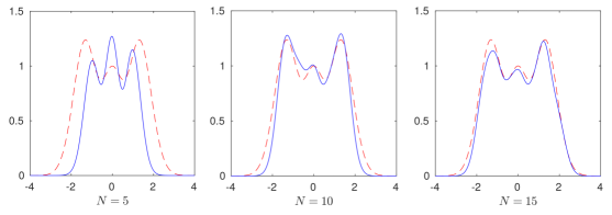
Figure 1: Reconstruction of $\gamma,$ given by equation (34), for increasing number of Fourier coefficients.

5.1. Examples with depth-dependent coefficients (see subsection 4.1)

In the following figures the true curve is represented by a dashed red line and the reconstructed by a solid blue line. Let $x\in\mathbbm{R}.$ In the first example we consider

$$\gamma(x)=(2x^{4}+1)\,\mathrm{e}^{-x^{2}},$$ (34)

and

$$\operatorname{\Im m}(\psi(\omega,x))=h_{1}(\omega)(x^{4}+x^{3}+x^{2}+0.1)\,\mathrm{e}^{-2x^{2}}.$$

We set $\Omega=[-3.5,3.5]$ and $\Omega_{L}=[-4,4]$ such that $\operatorname{supp}\psi(\omega,\cdot)\subset\Omega,$ and $\operatorname{supp}\gamma\subset\Omega_{L},$ and we restrict ourselves to $\omega\in\mathcal{W}:=[-4,4].$ We consider data with $\delta_{p}=\delta_{m}=3\%$ noise. The results are presented in Figure 1 for regularization parameter $\lambda=10^{-4}$ and different values of $N.$ Here, we see the improvement in the reconstructions as $N$ increases.

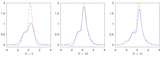
Figure 2: Reconstruction of $\gamma,$ given by equation (35), for increasing number of Fourier coefficients.

In the second example, we use the same function $\psi$ and we consider as $\gamma$ the function

$$\gamma(x)=h_{0}(x)+h_{0}(2x)+h_{1}(3x).$$ (35)

We keep all the parameters the same as in the first example. In Figure 2, we see the reconstructions for different number of coefficients.

In the third example, we consider

$$\operatorname{\Im m}(\psi(\omega,x))=(h_{1}(\omega)+h_{1}(2\omega))(x^{2}+0.1)\,\mathrm{e}^{-2x^{2}},$$ (36)

such that again $\operatorname{supp}\psi(\omega,\cdot)\subset[-3.5,3.5],$ see the left picture in Figure 3. We present the reconstructions of $\operatorname{\Im m}(\psi)$ using the form (34) for $\gamma,$ while keeping all the other parameters the same. We set $N=15$ coefficients. We present the results for $\operatorname{\Im m}(\psi(\omega,1)),\,\omega\in\mathcal{W},$ (center picture) and $\operatorname{\Im m}(\psi(3,x)),\,x\in\Omega,$ (right picture) in Figure 3.

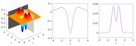
Figure 3: Reconstruction of $\operatorname{\Im m}(\psi),$ see equation (36), for $N=15$. The true imaginary part (left), the cross section of the reconstruction at the line $x=1$ (center) and at the line $\omega=3$ (right).

5.2. Examples with coefficients constant in one direction (see subsection 4.2)

Here, the measurements are given at points on a line. We consider the minimum amount of measurement points in order to have an exactly determined system (32) in our examples. In the following examples we keep the same noise levels $\delta_{p}=\delta_{m}=3\%$ and we obtain the regularization parameter using the L-curve criterion [18].

Let $x,y\in\mathbbm{R}.$ In the fourth example, we consider

$$\gamma(x,y)=\mathrm{e}^{-(x+1.5)^{2}-(y+1.5)^{2}},$$ (37)

and

$$\operatorname{\Im m}(\psi(\omega,x,y))=0.7(h_{1}(\omega)+h_{1}(2\omega))\,\mathrm{e}^{-(x+1.6)^{4}-\tfrac{1}{2}(y+1.6)^{4}}.$$ (38)

We set $\Omega=[-4,4]^{2},\,\Omega_{L}=[-4.5,4.5]^{2}$ and $\mathcal{W}=[-3,3].$ The reconstructions of $\gamma$ for $N=5$ and $\vartheta^{(1)}=(0,\,0,\,1)^{\top}$ are presented in Figure 4. The results for the cross-section of the imaginary part of $\psi$, given by equation (38), at frequency $\omega=0$ are presented in Figure 5.

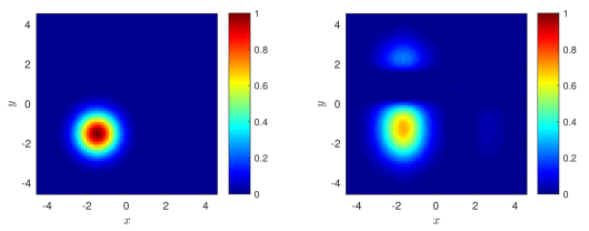
Figure 4: The exact function $\gamma,$ see equation (37), (left) and the reconstructed for $N=5$ and one measurement point (right).

In the last example the unknown function is given by

$$\gamma(x,y)=\mathrm{e}^{-(x+0.5)^{2}-(y+2)^{2}}+0.8\,\mathrm{e}^{-(x+2)^{2}-(y+0.5)^{2}}+\mathrm{e}^{-(x-2)^{2}-(y-2)^{2}}.$$ (39)

The size of the medium is kept the same as in the previous example and we set $\mathcal{W}=[-2,2]$. Here, we want to test the performance of our numerical scheme with respect to the number of the detection directions $\vartheta^{(k)}.$ In the case of three measurement directions, see (32), we consider

$$\vartheta^{(1)}=\left(0,\,\cos(\tfrac{5\pi}{12}),\,\sin(\tfrac{5\pi}{12})\right)^{\top},\quad\vartheta^{(2)}=\left(0,\,0,\,1\right)^{\top},\quad\vartheta^{(3)}=\left(0,\,-\cos(\tfrac{5\pi}{12}),\,\sin(\tfrac{5\pi}{12})\right)^{\top}.$$

The reconstructions for $N=5$ coefficients are presented in Figure 6, where we set to zero the negative values. We set the imaginary part of $\psi$ to be

$$\operatorname{\Im m}(\psi(\omega,x,y))=h_{1}(\omega)\left(\mathrm{e}^{-(x+0.5)^{4}-(y+2)^{4}}+\mathrm{e}^{-0.6(x+2)^{4}-(y+0.5)^{4}}+0.8\,\mathrm{e}^{-(x-2)^{4}-(y-2)^{4}}\right).$$ (40)

The reconstruction for $\mathcal{W}=[-3,3]$ are given in Figure 7, where we see the improvement of the results with respect to the Fourier coefficients. In the first case we set $N=5$ and we consider one detection direction. In the second case, we use $N=10$ coefficients and two measurement points in the directions:

$$\vartheta^{(1)}=\left(0,\,\cos(\tfrac{7\pi}{16}),\,\sin(\tfrac{7\pi}{16})\right)^{\top},\quad\vartheta^{(2)}=\left(0,\,-\cos(\tfrac{7\pi}{16}),\,\sin(\tfrac{7\pi}{16})\right)^{\top}.$$

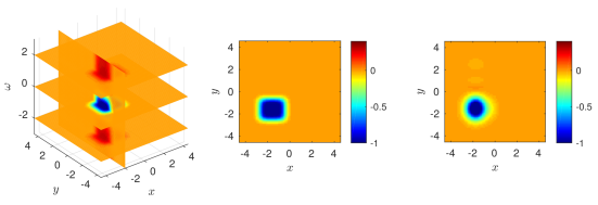
Figure 5: Reconstruction of $\operatorname{\Im m}(\psi),$ given by equation (38), for $N=5$. The true imaginary part (left), the cross section of the true value at the plane $\omega=0$ (center) and the reconstructed (right).

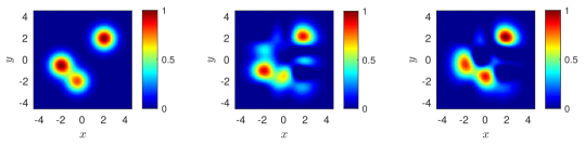
Figure 6: The exact function $\gamma,$ see equation (39), (left) and the reconstructed for $N=5$ and one measurement point $K=1$ (center) and $K=3$ (right).

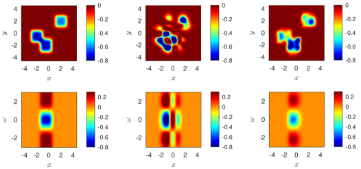
Figure 7: Reconstruction of $\operatorname{\Im m}(\psi),$ see equation (40). In the left column we see the cross-section of the true imaginary part at the plane $\omega=0$ (first row) and at the plane $y=-2$ (second row). The reconstructions for $N=5$ and one detection direction are presented in the second column. The results in the third column are for $N=10$ and two detection directions.

6. Conclusions

In this work we considered the inverse problem to reconstruct quantitatively the electric susceptibility and the Grüneisen parameter of a non-magnetic linear dielectric medium from measurements with the multi-modal tomographic system of Photoacoustic and Optical Coherence Tomography. Our scheme is based on the numerical solution of a Fredholm integral equation of the first kind for the Grüneisen parameter using a Galerkin type method. We presented numerical results for different kinds of media.

Appendix

We recall Hermite functions and we present their properties which are used in this work. We connect the Fourier and Hilbert transforms of a function with expansions in terms of Hermite functions.

Let $x\in\mathbbm{R}.$ The normalized Hermite functions $h_{k},\,k\in\mathbbm{N}_{0}$ are eigenfunctions of the inverse Fourier transform

$$\check{f}(x)=\frac{1}{2\pi}\int_{\mathbbm{R}}\hat{f}(\omega)\mathrm{e}^{-\mathrm{i}\omega t}\,\mathrm{d}\omega,$$

meaning they satisfy

$$\check{h}_{k}(x)=(-\mathrm{i})^{k}h_{k}(x).$$

The product of two Hermite polynomials admits the following series expansion

$$H_{k}(x)H_{l}(x)=k!l!\sum_{m=0}^{\min(k,l)}\frac{2^{m}}{m!(k-m)!(l-m)!}H_{k+l-2m}(x),$$

also known as Feldheim’s identity. Using (16) we see that the product of two Hermite functions can be written as

$$h_{k}(x)h_{l}(x)=\mathrm{e}^{-\tfrac{x^{2}}{2}}\sum_{m=0}^{\min(k,l)}\beta_{k,l,m}h_{k+l-2m}(x),$$ (41)

for

$$\beta_{k,l,m}=\pi^{-\tfrac{1}{4}}\frac{(k!l!(k+l-2m)!)^{\tfrac{1}{2}}}{m!(k-m)!(l-m)!}$$

We recall the addition formula [13, 24]

$$H_{k}(x+y)=\sum_{m=0}^{k}\frac{k!}{(k-m)!m!}(2y)^{k-m}H_{m}(x),$$ (42)

the multiplication formula

$$H_{k}(\rho x)=k!\sum_{m=0}^{\left[\tfrac{k}{2}\right]}\frac{\rho^{k}}{m!(k-2m)!}\left(1-\frac{1}{\rho^{2}}\right)^{m}H_{k-2m}(x),$$

and the inverse explicit expression

$$x^{k}=\frac{k!}{2^{k}}\sum_{m=0}^{\left[\tfrac{k}{2}\right]}\frac{1}{m!(k-2m)!}H_{k-2m}(x).$$ (43)

Let $f\in L^{2}(\mathbbm{R}).$ We consider the expansion

$$f(x)=\sum_{k=0}^{\infty}f_{k}h_{k}(x),$$

where the coefficients $f_{k}$ are defined by

$$f_{k}=\int_{\mathbbm{R}}f(x)h_{k}(x)\,\mathrm{d}x.$$

The Hilbert transform of $f$ admits the expansion

$$\mathcal{H}[f](x)=\sum_{k=0}^{\infty}\tilde{f}_{k}h_{k}(x),$$ (44)

where $\tilde{f}_{k}$ are given by [26]

$$\tilde{f}_{k}=(-\mathrm{i})^{k+1}\sum_{m=0}^{\infty}f_{m}(-\mathrm{i})^{m}\int_{\mathbbm{R}}\operatorname{sign}(x)h_{k}(x)h_{m}(x)\,\mathrm{d}x.$$ (45)

For $\bm{k}\in\mathbbm{N}_{0}^{d}$ and $x\in\mathbbm{R}^{d},$ we define the $\bm{k}$th Hermite polynomial as

$$H_{\bm{k}}(x)=\prod_{j=1}^{d}H_{k_{j}}(x_{j}).$$ (46)

Now we present the proof of Lemma 4.1.

Proof (Lemma 4.1):

We consider the convolution theorem for the inverse Fourier transform and the above properties.

$$\int_{\mathbbm{R}}\mathrm{e}^{-\tfrac{x^{2}}{2}}h_{k}(x)\mathrm{e}^{-\mathrm{i}\omega x}\,\mathrm{d}x =\left(\int_{\mathbbm{R}}\mathrm{e}^{-\tfrac{x^{2}}{2}}\mathrm{e}^{-\mathrm{i}\omega x}\,\mathrm{d}x\right)\ast\check{h}_{k}(\omega)$$

$$=2\pi(-\mathrm{i})^{k}\mathrm{e}^{-\tfrac{\omega^{2}}{2}}\ast h_{k}(\omega)$$

$$=2\pi(-\mathrm{i})^{k}\int_{\mathbbm{R}}\mathrm{e}^{-\tfrac{(\omega-y)^{2}}{2}}h_{k}(y)\,\mathrm{d}y$$

$$=2\pi(-\mathrm{i})^{k}\alpha_{k}\mathrm{e}^{-\tfrac{\omega^{2}}{4}}\int_{\mathbbm{R}}\mathrm{e}^{-(y-\tfrac{\omega}{2})^{2}}H_{k}(y)\,\mathrm{d}y$$

$$=2\pi(-\mathrm{i})^{k}\alpha_{k}\mathrm{e}^{-\tfrac{\omega^{2}}{4}}\int_{\mathbbm{R}}\mathrm{e}^{-z^{2}}H_{k}(z+\tfrac{\omega}{2})\,\mathrm{d}z.$$

To compute the last integral we apply the formula (42)

$$\int_{\mathbbm{R}}\mathrm{e}^{-z^{2}}H_{k}(z+\tfrac{\omega}{2})\,\mathrm{d}z =\sum_{m=0}^{k}\frac{k!}{(k-m)!m!}\omega^{k-m}\int_{\mathbbm{R}}\mathrm{e}^{-z^{2}}H_{m}(z)\,\mathrm{d}z$$

$$=\sum_{m=0}^{k}\frac{k!}{(k-m)!m!}\omega^{k-m}\int_{\mathbbm{R}}\mathrm{e}^{-z^{2}}H_{m}(z)H_{0}(z)\,\mathrm{d}z$$

$$=\sum_{m=0}^{k}\frac{k!}{(k-m)!m!}\omega^{k-m}a_{m}^{-2}\delta_{m,0}$$

$$=\sqrt{\pi}\omega^{k}.$$

The last two equations result to (20).

References

References

- [1] S. Arridge and O Scherzer “Imaging from coupled physics” In Inverse Probl. 28.8 IOP Publishing, 2012, pp. 080201 DOI: 10.1088/0266-5611/28/8/080201
- [2] G. Bal “Hybrid inverse problems and internal functionals” In Inverse Problems and Applications: Inside Out II 60, Mathematical Sciences Research Institute Publications Cambridge: Cambridge University Press, 2012, pp. 325–368
- [3] G. Bal and K. Ren “Multi-source quantitative photoacoustic tomography in a diffusive regime” In Inverse Problems 27.7, 2011, pp. 075003 DOI: 10.1088/0266-5611/27/7/075003
- [4] G. Bal, K. Ren, G. Uhlmann and T. Zhou “Quantitative thermo-acoustics and related problems” In Inverse Problems 27, 2011, pp. 055007
- [5] G. Bal and G. Uhlmann “Reconstructions for some coupled-physics inverse problems” In Applied Mathematics Letters 25.7, 2012, pp. 1030–1033 DOI: 10.1016/j.aml.2012.03.005
- [6] G. Bal and T. Zhou “Hybrid inverse problems for a system of Maxwell’s equations” In Inverse Problems 30, 2014, pp. 055013
- [7] M.. Brezinski “Optical Coherence Tomography Principles and Applications” New York: Academic Press, 2006
- [8] D. Colton and R. Kress “Inverse acoustic and electromagnetic scattering theory” 93, Applied Mathematical Sciences Berlin: Springer-Verlag, 1998
- [9] W. Drexler and J.. Fujimoto “Optical Coherence Tomography: Technology and Applications” Switzerland: Springer International Publishing, 2015
- [10] W. Drexler et al. “Optical coherence tomography today: speed, contrast, and multimodality” In Journal of Biomedical Optics 19.7 SPIE, 2014, pp. 071412
- [11] P. Elbau, L. Mindrinos and O. Scherzer “Inverse problems of combined photoacoustic and optical coherence tomography” In Math. Methods Appl. Sci. 40.3, 2017, pp. 505–522 DOI: 10.1002/mma.3915
- [12] P. Elbau, L. Mindrinos and O. Scherzer “Mathematical Methods of Optical Coherence Tomography” In Handbook of Mathematical Methods in Imaging Springer New York, 2015, pp. 1169–1204 DOI: 10.1007/978-1-4939-0790-8˙44
- [13] E. Feldheim “Relations entre les polynomes de Jacobi, Laguerre et Hermite” In Acta Mathematica 75, 1943, pp. 117–138
- [14] A.. Fercher “Optical coherence tomography” In Journal of Biomedical Optics 1.2 SPIE, 1996, pp. 157–173
- [15] D.. Friedrich “Two-photon molecular spectroscopy” In Journal of Chemical Education 59.6, 1982, pp. 472 DOI: 10.1021/ed059p472
- [16] W. Hackbusch “Integral Equations. Theory and Numerical Treatment” Basel: Birkhäuser, 1995
- [17] M. Haltmeier, O. Scherzer, P. Burgholzer and G. Paltauf “Thermoacoustic computed tomography with large planar receivers” In Inverse Probl. 20.5, 2004, pp. 1663–1673 DOI: 10.1088/0266-5611/20/5/021
- [18] P.. Hansen and D.. O’Leary “The Use of the L-Curve in the Regularization of Discrete Ill-Posed Problems” In SIAM Journal on Scientific Computing 14.6, 1993, pp. 1487–1503 DOI: 10.1137/0914086
- [19] R. Kress “Linear Integral Equations” Berlin: Springer Verlag, 1999
- [20] P. Kuchment “Mathematics of hybrid imaging: a brief review” In The Mathematical Legacy of Leon Ehrenpreis Berlin: Springer, 2012, pp. 183–208
- [21] M. Liu et al. “Combined multi-modal photoacoustic tomography, optical coherence tomography (OCT) and OCT angiography system with an articulated probe for in vivo human skin structure and vasculature imaging” In Biomedical Optics Express 7.9 OSA, 2016, pp. 3390–3402
- [22] M. Liu et al. “In vivo spectroscopic photoacoustic tomography imaging of a far red fluorescent protein expressed in the exocrine pancreas of adult zebrafish” In Proceedings of SPIE 8943, 2014, pp. 142
- [23] M. Liu et al. “In vivo three dimensional dual wavelength photoacoustic tomography imaging of the far red fluorescent protein E2-Crimson expressed in adult zebrafish” In Biomedical Optics Express 4.10 OSA, 2013, pp. 1846–1855
- [24] W. Magnus, F. Oberhettinger and R.P. Soni “Formulas and Theorems for the Special Functions of Mathematical Physics” Berlin Heidelberg: Springer, 1966
- [25] A. Polyanin and A. Manzhirov “Handbook of Integral Equations”, Mathematics in Science and Engineering London, New York, Washington D.C.: CRC Press, 1998
- [26] I. Porras, C.. Schuster and F.. King “Convergence Accelerator Approach to the Numerical Evaluation of Hilbert Transforms Based on Expansions in Hermite Functions” In International Journal of Applied Mathematics 41.3, 2013, pp. 252–259
- [27] K. Ren and R. Zhang “Nonlinear quantitative photoacoustic tomography with two-photon absorption”, 2016
- [28] L.. Wang “Prospects of photoacoustic tomography” In Medical Physics 35.12 American Association of Physicists in Medicine, 2008, pp. 5758–5767 DOI: 10.1118/1.3013698
- [29] T. Widlak and O. Scherzer “Hybrid tomography for conductivity imaging” In Inverse Probl. 28.8 IOP Publishing Ltd, 2012, pp. 084008 DOI: 10.1088/0266-5611/28/8/084008
- [30] M. Xu and L.. Wang “Photoacoustic imaging in biomedicine” In Review of Scientific Instruments 77.4, 2006 DOI: 10.1063/1.2195024
- [31] E.. Zhang et al. “Multimodal photoacoustic and optical coherence tomography scanner using an all optical detection scheme for 3D morphological skin imaging” In Journal of Biomedical Optics 2.8 SPIE, 2011, pp. 2202–2215 DOI: 10.1364/BOE.2.002202