Approximate Likelihood Approaches for Detecting the Influence of Primordial Gravitational Waves in Cosmic Microwave Background Polarization

Abstract

One of the major targets for next-generation cosmic microwave background (CMB) experiments is the detection of the primordial B-mode signal. Planning is under way for Stage-IV experiments that are projected to have instrumental noise small enough to make lensing and foregrounds the dominant source of uncertainty for estimating the tensor-to-scalar ratio $r$ from polarization maps. This makes delensing a crucial part of future CMB polarization science. In this paper we present a likelihood method for estimating the tensor-to-scalar ratio $r$ from CMB polarization observations, which combines the benefits of a full-scale likelihood approach with the tractability of the quadratic delensing technique. This method is a pixel space, all order likelihood analysis of the quadratic delensed B modes, and it essentially builds upon the quadratic delenser by taking into account all order lensing and pixel space anomalies. Its tractability relies on a crucial factorization of the pixel space covariance matrix of the polarization observations which allows one to compute the full Gaussian approximate likelihood profile, as a function of $r$, at the same computational cost of a single likelihood evaluation.

I Introduction

The inflation paradigm has successfully explained the origin of primordial density perturbations that grew into the Cosmic Microwave Background (CMB) anisotropies and large scale structure we observe (e.g. Mukhanov and Chibisov, 1981; Guth, 1981; Linde, 1982; Albrecht and Steinhardt, 1982; Lidsey et al., 1997; Lyth and Riotto, 1999). A key prediction of inflation is the background of primordial gravitational waves (GWs) or tensor-mode perturbations (e.g. Starobinskii, 1979; Rubakov et al., 1982; Fabbri and Pollock, 1983; Abbott and Wise, 1984; Starobinskii, 1985), which imprints a unique polarization pattern, called a primordial B mode, on the CMB anisotropies Stebbins (1996); Kamionkowski et al. (1997a, b); Seljak and Zaldarriaga (1997); Seljak (1997); Zaldarriaga and Seljak (1997). Further, detection of a nearly scale-invariant background of GWs would severely challenge non-inflationary models (e.g. Khoury et al., 2001a, b, 2003; Steinhardt and Turok, 2002; Boyle et al., 2004). The strength of primordial gravitational waves or tensor-mode power is commonly quantified by the tensor-to-scalar ratio $r$. Joint analysis of BICEP2/Keck Array and Planck data yields an upper bound $r<0.12$ at $95\%$ confidence level (BICEP2/Keck Array and Planck Collaborations, 2015), the bound is slightly tightened when the Planck high-$\ell$ polarization data are included (Planck Collaboration XX, 2016), and BICEP2/Keck Collaboration gives the latest upper bound $r<0.09$ at $95\%$ confidence level (BICEP2/Keck Array Collaborations, 2016). Fourth generation experiments, including COrE, LiteBird, and CMB Stage-IV, are expected to constrain $r$ with uncertainty $\sigma(r)\simeq 0.001$ (COrE Collaboration, 2011; LiteBird Collaboration, 2014; Ishino et al., 2016; CMB-S4 Collaboration, 2016; Cabass et al., 2016; Kamionkowski and Kovetz, 2016; Delabrouille et al., 2017).

The primordial B modes are contaminated by several sources: emission from galactic dust and other foregrounds Hildebrand et al. (1999); Draine (2004); Benoît et al. (2004); Mortonson et al. (2014); Niemack et al. (2015); Planck Collaboration XXX (2016); Planck Collaboration L (2016); Krachmalnicoff et al. (2016), instrumental noise, and gravitational lensing of scalar CMB perturbations. The B modes generated by gravitational lensing of the CMB have been detected (Hanson et al., 2013; POLARBEAR Collaboration, 2014; van Engelen et al., 2015; Story et al., 2015; BICEP2/Keck Array and Planck Collaborations, 2015; Planck Collaboration XV, 2016). The lensed B-mode power spectrum is nearly a constant at small multipoles ($\ell\lesssim 1000$) and therefore manifests as an effective white noise with amplitude $\sim 5$ $\mu$K-arcmin (Lewis and Challinor, 2006; Sherwin and Schmittfull, 2015). For CMB Stage-IV, we expect to decrease the instrumental noise to $\sim 1\ \mu$K-arcmin (CMB-S4 Collaboration, 2016). Then, the lensing B noise (and foregrounds) would become the dominant noise source limiting the primordial B-mode survey.

Fortunately, the lensing B noise is well understood. Up to leading order, one can effectively delense observed B modes by utilizing a quadratic combination of observed E modes and an estimate of the lensing potential field $\phi^{\rm est}$ (Knox and Song, 2002; Kesden et al., 2002; Seljak and Hirata, 2004; Simard et al., 2015; Sherwin and Schmittfull, 2015). We find that the validity of the quadratic delenser crucially depends on a partial cancellation of higher order lensing terms (see Section IV.3 for details). However, in the regime of low instrumental noise and small lensing potential field estimate uncertainty, higher-order lensing terms, ignored by the quadratic delensing technique, can have an appreciable effect. These higher order terms not only induce a delensing bias but also contain information on primordial B modes. In addition, experimental complexities such as non-stationary noise and sky cuts become non-trivial for spectral based methods such as the quadratic delenser.

As an alternative, a full-scale likelihood analysis of the tensor-to-scalar ratio $r$ can, in principle, optimally account for all the Gaussian and non-Gaussian information in the CMB observations. Unfortunately, a full likelihood analysis requires computation resources beyond what is available in the near future. In this paper, we introduce a likelihood approximation which is modified from the full-scale likelihood, so as to be computationally tractable.

We start with introducing a Gaussian likelihood incorporating all the 2-point information. A key element of our likelihood analysis is the covariance matrix of the polarization maps. For each data pair ($d_{i},d_{j}$) ($d$ can be $Q$ or $U$), its covariance depends on the primordial polarization power spectra $C_{\ell}^{EE}$ and $C_{\ell}^{BB,r}$, lensing potential field $\phi(x)$ (and instrumental noise $N^{QQ}$ and $N^{UU}$), where the E-mode power $C_{\ell}^{EE}$ has been well constrained (e.g. Planck Collaboration XI, 2016; Planck Collaboration XIII, 2016), while the primordial B-mode signal has not been detected. Following the prediction of the inflation paradigm, we assume the tensor perturbations to be scale-invariant and Gaussian. Hence all the primordial B-mode information is encoded in the single parameter $r$, the tensor-to-scalar ratio at $k=0.05$ Mpc^-1. Then the covariance matrix $\tilde{\Sigma}_{r,\phi}$ depends on the unknown parameter $r$ and the underlying lensing potential field $\phi(x)$, where $\phi(x)$ can be estimated from exterior tracers, e.g. cosmic infrared background (CIB) (Song et al., 2003; Dole et al., 2006; Planck Collaboration XVII, 2014; Planck Collaboration XV, 2016; Larsen et al., 2016; Manzotti et al., 2017) or from intrinsic CMB via, e.g. quadratic estimators (Hu, 2001; Hu and Okamoto, 2002) or Bayesian approach (Hirata and Seljak, 2003a, b; Anderes et al., 2011, 2015; Millea et al., 2017). We obtain a covariance matrix $\Sigma_{r}$ depending only on $r$ by marginalizing $\tilde{\Sigma}_{r,\phi}$ over uncertainties in the lensing potential field estimate $\phi^{\rm est}$. With this full covariance matrix $\Sigma_{r}$, it is then straightforward to compute the likelihood of $r$ for given data vector $d$ by approximating $d$ as a Gaussian vector.

In principle, this Gaussian likelihood method can exploit all the 2-point $r$ information from the polarization maps, but usually the computation resource demands are still excessive. For example, to constrain $r$ from some polarization maps with $p$ pixels, we need to compute the full likelihood profile $L(r|d)$ as a function of $r$, which in practice requires computing the likelihood on a range of $r$ values, say $50$ values evenly distributed in the interval $[0,0.2]$. For each different $r$, we need to compute the quadratic form $d^{\intercal}\Sigma_{r}^{-1}d$ and the determinant $\det(\Sigma_{r})$, due to the $r$ dependence of the covariance matrix. In any realistic experiments with $p\gtrsim 10^{4}$, it is a huge amount of work to compute and invert the covariance matrix of dimension $2p\times 2p$ for that many $r$ values, where the factor $2$ comes from two observables $Q$ and $U$ on each pixel.

In this paper, we present a modified Gaussian likelihood tailoring the full-scale likelihood analysis so as to be computationally tractable. The method consists of two parts. In the first part, we decompose the covariance matrix $\Sigma_{r}$ as $\Sigma^{\rm en}+r\Sigma^{\rm b}$, where $\Sigma^{\rm en}$ is the contribution from E modes and instrumental noise, and $r\Sigma^{\rm b}$ is the contribution from B modes. This decomposition allows us to compute the covariance $\Sigma_{r}$, as a function of $r$, at the same computational cost of a single covariance matrix computation. In the second part, we suppress data size by tracking only $s$ high signal-to-noise modes, say the large-scale quadratic delensed B modes. We project out the lensing-generated B modes and obtain the delensed modes $B^{\rm del}$ from the polarization data $d$ via a projection matrix $v$, $(^{0}B^{\rm del}_{\bm{\ell}})_{s}=(v^{\intercal})_{s\times 2p}d_{2p}$, with $s\sim 500$ and the upper left index ⁰ denoting the projected data vector limited to the $s$ lowest frequency modes available. Then, the covariance matrix of the projected data vector ${}^{0}B^{\rm del}_{\bm{\ell}}$ is given by $v^{\intercal}\Sigma_{r}v$, with which the computation of the $r$ likelihood $L(r|^{0}B^{\rm del}_{\bm{\ell}})$ given the projected data vector turns out to be tractable. This method can be naturally extended to incorporate higher frequency modes, as we describe in Section III.

The paper is organized as follows. We introduce the quadratic delenser and the likelihood based delenser in Section II and Section III, respectively. In Section IV, we apply the two $r$ constraining techniques on simulations mimicking Stage III and IV CMB surveys, and compare their $r$ constraints. We conclude with Section V. For reference, we derive the analytic expression for the covariance matrices of the polarization maps, and the eigenvalue method for inverting large matrices in Appendices A, B and C, respectively.

II Quadratic Delenser

For simplicity, we assume no contamination of foregrounds throughout this paper. Then the observed B modes can generally be expressed as

$$B^{\rm obs}=B^{r}+B^{\rm len}+N^{B},$$ (1)

where $B^{r},B^{\rm len},N^{B}$ are primordial B signal, lensing B noise and instrumental B noise, respectively. To constrain the primordial B signal, delensing is essential, where we obtain an estimate of the lensing B noise and subtract it off from the observed B modes. Here we introduce a quadratic delenser.

Accurate to the leading order of the lensing potential $\phi_{\bm{\ell}}$, $B^{\rm len}$ is the convolution of the lensing potential and primordial E modes, i.e.,

$$B^{\rm len}_{\bm{\ell}}=\int\frac{d^{2}\bm{\ell}^{\prime}}{2\pi}\bm{\ell}^{\prime}\cdot(\bm{\ell}-\bm{\ell}^{\prime})\sin(2\varphi_{\bm{\ell},\bm{\ell}^{\prime}})E_{\bm{\ell}^{\prime}}\phi_{\bm{\ell}-\bm{\ell}^{\prime}}.$$ (2)

Usually, the underlying lensing potential is not known a priori, but can be estimated from either intrinsic CMB or from external tracers. From an estimated lensing potential $\phi^{\rm est}_{\bm{\ell}}$ and observed modes $E_{\bm{\ell}}^{\rm obs}$, we construct a quadratic estimate of the lensing B noise

$$B^{\rm len,est}_{\bm{\ell}}=\int\frac{d^{2}\bm{\ell}^{\prime}}{2\pi}f_{\bm{\ell},\bm{\ell}^{\prime}}\bm{\ell}^{\prime}\cdot(\bm{\ell}-\bm{\ell}^{\prime})\sin(2\varphi_{\bm{\ell},\bm{\ell}^{\prime}})E^{\rm obs}_{\bm{\ell}^{\prime}}\phi^{\rm est}_{\bm{\ell}-\bm{\ell}^{\prime}},$$ (3)

where $\varphi_{\bm{\ell},\bm{\ell}^{\prime}}=\varphi_{\bm{\ell}}-\varphi_{\bm{\ell}^{\prime}}$, $E^{\rm obs}$ is the observed E modes (to the lowest order, the difference between lensed E and primordial E can be neglected), and the weighting function $f_{\bm{\ell},\bm{\ell}^{\prime}}$ is to be determined by minimizing the residual, $B_{\bm{\ell}}^{\rm res}=B^{\rm len}_{\bm{\ell}}-B^{\rm len,est}_{\bm{\ell}}$. If we define the correlation coefficient of $\phi_{\bm{\ell}}$ and $\phi^{\rm est}_{\bm{\ell}}$

$$\rho_{\ell}=\frac{C_{\ell}^{\phi,\phi^{\rm est}}}{\sqrt{C_{\ell}^{\phi\phi}C_{\ell}^{\phi^{\rm est}\phi^{\rm est}}}},$$ (4)

the optimal weight at leading order was proved to be (Sherwin and Schmittfull, 2015)

$$f_{\bm{\ell},\bm{\ell}^{\prime}}=\frac{C_{l^{\prime}}^{EE}}{C_{l^{\prime}}^{EE}+N_{l^{\prime}}^{EE}}\rho_{|\bm{\ell}-\bm{\ell}^{\prime}|}^{2},$$ (5)

which enables a minimal residual power spectrum

$$C_{\bm{\ell}}^{BB,{\rm res}} =\int\frac{d^{2}\bm{\ell}^{\prime}}{(2\pi)^{2}}\left[\bm{\ell}^{\prime}\cdot(\bm{\ell}-\bm{\ell}^{\prime})\sin(2\varphi_{\bm{\ell},\bm{\ell}^{\prime}})\right]^{2}$$ (6)

$$\times C_{\bm{\ell}^{\prime}}^{EE}C^{\phi\phi}_{\bm{\ell}-\bm{\ell}^{\prime}}(1-f_{\bm{\ell},\bm{\ell}^{\prime}}).$$

After subtracting off the template $B_{\bm{\ell}}^{\rm len,est}$, we obtain a quadratic delensed B-mode map

$$B_{\bm{\ell}}^{\rm del}=B_{\bm{\ell}}^{\rm obs}-B_{\bm{\ell}}^{\rm len,est}=B_{\bm{\ell}}^{r}+B_{\bm{\ell}}^{\rm res}+N_{\bm{\ell}}^{B},$$ (7)

and its power spectrum

$$C_{\ell}^{BB,{\rm del}}=C_{\ell}^{BB,r}+C_{\ell}^{BB,{\rm res}}+N^{BB}_{\ell}.$$ (8)

From the delensed B modes, one can better constrain $r$ due to the suppressed lensing B noise. Note that in the evaluation of the residual lensing B power $C_{\ell}^{BB,{\rm res}}$ of Eq. (6) we have made two approximations: 1) we keep only the linear order lensing in $B^{\rm len}$; 2) we completely ignore the lensing in $E^{\rm obs}$.

III Gaussian Likelihood Delenser

In contrast to the quadratic delenser, the likelihood analysis works on observables $Q^{\rm obs}$ and $U^{\rm obs}$ in pixel space. Concatenating the polarization data on all pixels yields a length-$2p$ data vector

$$d=[Q^{\rm obs}(x_{1})\cdots Q^{\rm obs}(x_{p}),U^{\rm obs}(x_{1})\cdots U^{\rm obs}(x_{p})]^{\intercal},$$ (9)

with $p$ being the number of pixels. We first evaluate the covariance matrix of the data vector, which depends on the primordial polarization power spectra $C_{\ell}^{EE}$ and $C_{\ell}^{BB,r}$, lensing potential field $\phi(x)$ (and instrumental noise). With $C_{\ell}^{EE}$ being well-determined, and $C_{\ell}^{BB,r}$ being parametrized by the tensor-to-scalar ratio $r$, we marginalize the covariance matrix $\tilde{\Sigma}_{r,\phi}$ over uncertainties in $\phi(x)$ estimate, and obtain a covariance matrix $\Sigma_{r}$ depending only on $r$. Then it is straightforward to compute the approximate likelihood of $r$ for given data $d$ by approximating $d$ as a Gaussian vector, i.e.,

$$-2\log L(r|d)=d^{\intercal}\Sigma^{-1}_{r}d+\log\det\Sigma_{r},$$ (10)

up to a constant term.

III.1 Comparison with the Quadratic Delenser

Before delving into the details of the Gaussian likelihood delenser, it would be useful to do a brief comparison with the quadratic delenser (see Table 1):

• The Quadratic Delenser works on the delensed modes $B^{\rm del}_{\bm{\ell}}$ in Fourier space, and approximates these modes as stationary and Gaussian, i.e.,

  $$\begin{pmatrix}\vdots\\ B^{\rm del}_{\bm{\ell}}\\ \vdots\end{pmatrix}\sim N(0,\begin{bmatrix}\ddots&0&0\\ 0&C^{BB,\rm del}_{\ell}&0\\ 0&0&\ddots\end{bmatrix}),$$

  where the power spectrum $C^{BB,\rm del}_{\ell}$, derived in Eq. (8), only takes into account the leading-order in $\phi$. Therefore, the quadratic delenser exploits the 2-point information in a biased way by ignoring the non-stationarity and higher-order lensing in the power spectrum.

• The Gaussian Likelihood Delenser works on the observables $d$ in pixel space, and approximates the data vector $d$ as Gaussian after marginalizing over uncertainties in the $\phi$ estimate. In the computation of the covariance matrix $\Sigma_{r}$, all-order lensing is taken into account and no stationarity assumption is made. Therefore, the Gaussian likelihood delenser naturally incorporates all the 2-point information.

Delenser	Quadratic Delenser	Gaussian Likelihood
working space	Fourier	pixel
power spectrum / cov. matrix	leading order	all order
non-stationarity	✗	$\checkmark$
non-Gaussianity	✗	✗

Table 1: A brief comparison of the two delensers.

The Gaussian likelihood is potentially favored in several aspects, but usually is computationally excessive. As explained in the Introduction, the bottleneck of the likelihood analysis is the covariance matrix $\Sigma_{r}$ related computation, which is of large size $2p\times 2p$, and is a function of $r$. Here we introduce a modified Gaussian likelihood method. The method consists of two parts, covariance decomposition and data compression, where the former allows us to compute the covariance matrix $\Sigma_{r}$, as a function of $r$, at the computation cost of a single covariance matrix computation; and the latter allows us to compress the covariance matrix by tracking a small number of high $S/N$ modes.

III.2 Covariance Decomposition

To avoid repeating the computation of the covariance matrix $\Sigma_{r}$ for each different $r$, we find it is possible to single out the $r$ dependence by decomposing the covariance matrix as

$$\Sigma_{r}=\Sigma^{\rm en}+r\Sigma^{\rm b},$$ (11)

where $\Sigma^{\rm en}$ is the contribution from E modes and instrumental noise, and $r\Sigma^{\rm b}$ is the contribution from primordial B modes. With this decomposition, we can obtain the covariance matrix $\Sigma_{r}$ as a function of $r$, as long as the $r$-independent components $\Sigma^{\rm en}$ and $\Sigma^{\rm b}$ are obtained.

For the covariance decomposition of Eq. (11), we first decompose observables $Q^{\rm obs}$ and $U^{\rm obs}$ as linear combinations of E modes and B modes. Stokes parameters $Q$ and $U$ are related to coordinate independent quantities $E$ and $B$ via (Stebbins, 1996; Kamionkowski et al., 1997a, b; Seljak, 1997)

$$Q_{\bm{\ell}} =-\cos(2\varphi_{\bm{\ell}})E_{\bm{\ell}}+\sin(2\varphi_{\bm{\ell}})B_{\bm{\ell}},$$ (12)

$$U_{\bm{\ell}} =-\sin(2\varphi_{\bm{\ell}})E_{\bm{\ell}}-\cos(2\varphi_{\bm{\ell}})B_{\bm{\ell}}.$$

We define the following modulated E/B modes

$$SE_{\bm{\ell}} \equiv-\sin(2\varphi_{\bm{\ell}})E_{\bm{\ell}},\quad SB_{\bm{\ell}}\equiv+\sin(2\varphi_{\bm{\ell}})B_{\bm{\ell}},$$ (13)

$$CE_{\bm{\ell}} \equiv-\cos(2\varphi_{\bm{\ell}})E_{\bm{\ell}},\quad CB_{\bm{\ell}}\equiv-\cos(2\varphi_{\bm{\ell}})B_{\bm{\ell}},$$

then the observables $Q^{\rm obs}$ and $U^{\rm obs}$ are consequently expressed as

$$Q^{\rm obs}(x) =\widetilde{CE}(x)+\sqrt{r}\widetilde{SB^{0}}(x)+N^{Q}(x),$$ (14)

$$U^{\rm obs}(x) =\widetilde{SE}(x)+\sqrt{r}\widetilde{CB^{0}}(x)+N^{U}(x),$$

where $B^{0}$ denotes fiducial B modes with unity power spectrum $C_{\ell}^{BB,r=1}$, tildes denote lensed fields $\widetilde{X}(x)=X(x+\nabla\phi(x))$ ($X=CE,SE,CB,SB$), and $N^{Q,U}$ is the $Q/U$ noise.

With above decomposition, we find the data vector $d$ is Gaussian with covariance $\tilde{\Sigma}_{r,\phi}$ for given $r$ and $\phi(x)$, i.e., $d\sim N(0,\tilde{\Sigma}_{r,\phi})$, where

$$\tilde{\Sigma}_{r,\phi}\equiv\left[\begin{tabular}[]{cc}$\tilde{\Sigma}^{Q^{\rm obs},Q^{\rm obs}}$&$\tilde{\Sigma}^{Q^{\rm obs},U^{\rm obs}}$\\ $\tilde{\Sigma}^{Q^{\rm obs},U^{\rm obs}}$&$\tilde{\Sigma}^{U^{\rm obs},U^{\rm obs}}$\end{tabular}\right]_{r,\phi}$$ (15)

and the covariance matrix is naturally expressible in the form of Eq. (11), i.e.,

$$\tilde{\Sigma}^{Q^{\rm obs},Q^{\rm obs}} =\tilde{\Sigma}^{CE,CE}+r\tilde{\Sigma}^{SB^{0},SB^{0}}+\Sigma^{NQ,NQ},$$ (16)

$$\tilde{\Sigma}^{Q^{\rm obs},U^{\rm obs}} =\tilde{\Sigma}^{CE,SE}+r\tilde{\Sigma}^{SB^{0},CB^{0}},$$

$$\tilde{\Sigma}^{U^{\rm obs},U^{\rm obs}} =\tilde{\Sigma}^{SE,SE}+r\tilde{\Sigma}^{CB^{0},CB^{0}}+\Sigma^{NU,NU}.$$

In a more practical case, we only have an estimate of lensing potential $\phi_{\bm{\ell}}^{\rm est}$ which is a noisy version of the true $\phi_{\bm{\ell}}$, i.e., $\phi_{\bm{\ell}}^{\rm est}=\phi_{\bm{\ell}}+n^{\phi}_{\bm{\ell}}$, where $n^{\phi}_{\bm{\ell}}$ is the uncertainty of the $\phi$ estimate and its power spectrum $N_{\ell}^{\phi\phi}$ is usually an output of the lensing estimator used. For an unbiased estimator with Gaussian uncertainty, one can write $n^{\phi}_{\bm{\ell}}\sim N(0,N_{\ell}^{\phi\phi})$. Then the correlation coefficient of $\phi$ and $\phi^{\rm est}$ defined in Eq. (4) now is explicitly known as

$$\rho_{\ell}=\sqrt{\frac{C_{\ell}^{\phi\phi}}{C_{\ell}^{\phi\phi}+N_{\ell}^{\phi\phi}}}.$$ (17)

In this context, one can treat $\phi^{\rm est}$ as data and compute the posterior on $\phi$ given $\phi^{\rm est}$, i.e.,

$$P(\phi_{\bm{\ell}}|\phi^{\rm est}_{\bm{\ell}})\sim N\left(\mu\phi_{\bm{\ell}},C_{\ell}^{n\phi,n\phi}\right).$$ (18)

with

$$\mu\phi_{\bm{\ell}} =\frac{C_{\ell}^{\phi\phi}}{C_{\ell}^{\phi\phi}+N_{\ell}^{\phi\phi}}\phi_{\bm{\ell}}^{\rm est}=\rho_{\ell}^{2}\phi_{\bm{\ell}}^{\rm est},$$ (19)

$$C_{\ell}^{n\phi,n\phi} =\frac{C_{\ell}^{\phi\phi}}{C_{\ell}^{\phi\phi}+N_{\ell}^{\phi\phi}}N_{\ell}^{\phi\phi}=\rho_{\ell}^{2}N_{\ell}^{\phi\phi},$$

Therefore a sample $\phi_{\bm{\ell}}\sim P(\phi_{\bm{\ell}}|\phi^{\rm est}_{\bm{\ell}})$ can be writen as

$$\phi_{\bm{\ell}}=\mu\phi_{\bm{\ell}}+n\phi_{\bm{\ell}},$$ (20)

with $n\phi_{\bm{\ell}}\sim N(0,C_{\ell}^{n\phi,n\phi})$.

Marginalizing $\tilde{\Sigma}_{r,\phi}$ over $n\phi$, we obtain a covariance matrix only depending on $r$, i.e., $\Sigma_{r}\equiv\langle\tilde{\Sigma}_{r,\phi}\rangle_{n\phi}$, where its analytic form is presented in Appendices A and B. The computation of its inverse matrix $\Sigma_{r}^{-1}$ is presented in Appendix C.

III.3 Data Compression

III.3.1 idea

To compress the data, we project the original length-$2p$ data vector $d$ to a length-$s$ data ($s\sim 500$) via a projection matrix $v$, and apply the likelihood analysis on the projected data $\hat{d}_{s}=(v^{\intercal})_{s\times 2p}d_{2p}$. Let $\Sigma_{r}$ be the covariance matrix of data vector $d$, then $v^{\intercal}\Sigma_{r}v$ is the covariance matrix of projected data vector $\hat{d}$, i.e., $d\sim N\left(0,\Sigma_{r}\right)$, and $\hat{d}\sim N\left(0,v^{\intercal}\Sigma_{r}v\right)$. Then the likelihood of $r$ given projected data $\hat{d}$ is simply

$$-2\log L(r|\hat{d})=\hat{d}^{\intercal}(v^{\intercal}\Sigma_{r}v)^{-1}\hat{d}+\log\det(v^{\intercal}\Sigma_{r}v),$$ (21)

up to a constant term.

The goal is to find a projection matrix $v$ such that $\hat{d}$ is highly informative for $r$. Since the primordial B modes at large scales are less contaminated by the lensing B noise, a natural choice is to project the polarization data to the large-scale quadratic delensed modes defined in Equation (7), i.e., $\hat{d}^{0}=$ ${}^{0}B_{\bm{\ell}}^{\rm del}$, where the upper index ⁰ denotes the projected data vector limited to the $s$ lowest frequency modes available (Figure 1). The method can be naturally extended to higher frequency modes, $\hat{d}^{i}=\ ^{i}B^{\rm del}_{\bm{\ell}}$ $(i=1,2,\dots)$ with $\bm{\ell}$ running over the $s$ next/next-next/$\dots$ lowest frequency modes. With these projected data vectors $\hat{d}^{i}=\ ^{i}B^{\rm del}_{\bm{\ell}}=(v^{\intercal})^{i}d$, the total likelihood is given by

$$\log L(r|d)\approx\sum_{i=0}^{i_{\rm max}}\log L(r|\hat{d}^{i}),$$ (22)

assuming negligible correlation for different projected vectors. We will confirm the validity of ignoring the cross correlation via simulations in Section IV.

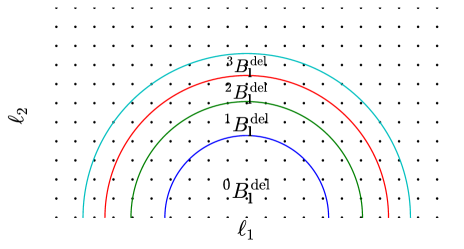
Figure 1: The modes covered by each different projected vector ${}^{i}B_{\bm{\ell}}^{\rm del}(i=0,1,2,\cdots)$. Here we only show the modes with $\ell_{2}\geq 0$, since our observables $Q^{\rm obs}$ and $U^{\rm obs}$ are real numbers.

We find that the modified Gaussian likelihood method works better if we incorporate the same number of E modes and delensed B modes in each projected vector, i.e.,

$$[\hat{d}^{i}]_{2s}=\begin{bmatrix}(^{i}B^{\rm del}_{\bm{\ell}})_{s}\\ (^{i}E^{\rm obs}_{\bm{\ell}})_{s}\end{bmatrix}=\begin{bmatrix}(v_{b}^{\intercal})^{i}_{s\times 2p}\\ (v_{e}^{\intercal})^{i}_{s\times 2p}\end{bmatrix}d_{2p}=(v^{\intercal})^{i}_{2s\times 2p}d_{2p}.$$ (23)

III.3.2 projection matrix

In this subsection, we focus on the computation of the projection matrix. As described in Section II, the quadratic delenser is actually a linear operator, i.e.,

$$d=(Q^{\rm obs},U^{\rm obs})^{\intercal} \xrightarrow{{\rm Eq.}(\ref{eq:queb})}(E^{\rm obs},B^{\rm obs}),$$ (24)

$$\xrightarrow{{\rm Eq.}(\ref{eq:wconvol})}(B^{\rm len,est},B^{\rm obs}),$$

$$\xrightarrow{{\rm Eq.}(\ref{eq:bdel})}B^{\rm obs}-B^{\rm len,est}=B^{\rm del}.$$

Therefore we can formally write the quadratic delensing as $(B^{\rm del}_{\bm{\ell}})_{2p}=\mathcal{P}_{2p\times 2p}d_{2p}$, where $\mathcal{P}$ is a concatenation of the three linear operations above, and its matrix elements can be found by recording the impulse response of the delensed modes to each element in the data vector. For example, we first do the quadratic delensing to a “data vector” $\delta_{1}=(1,0,\dots,0)^{\intercal}_{2p}$ and denote the corresponding delensed modes as $(B^{\rm del}_{\bm{\ell}}|_{\delta_{1}})$, i.e.,

$$(B^{\rm del}_{\bm{\ell}}|_{\delta_{1}})_{2p}=\mathcal{P}_{2p\times 2p}(\delta_{1})_{2p}=\textrm{1st col. of}\ \mathcal{P}.$$ (25)

where $(B^{\rm del}_{\bm{\ell}}|_{\delta_{1}})$ is obtained via delensing of Eq. (24). In this way, we obtain the matrix $\mathcal{P}$.

It is clear that the projection matrices of vectors ${}^{i}B^{\rm del}_{\bm{\ell}}$ correspond to row blocks of $\mathcal{P}$. Explicitly, we write $(B^{\rm del}_{\bm{\ell}})_{2p}=\mathcal{P}_{2p\times 2p}d_{2p}$ as

$$\begin{pmatrix}(^{0}B_{\bm{\ell}}^{\rm del})_{s}\\ (^{1}B_{\bm{\ell}}^{\rm del})_{s}\\ (^{2}B_{\bm{\ell}}^{\rm del})_{s}\\ \dots\end{pmatrix}=\mathcal{P}_{2p\times 2p}d_{2p}=\begin{pmatrix}(^{0}\mathcal{P})_{s\times 2p}\\ (^{1}\mathcal{P})_{s\times 2p}\\ (^{2}\mathcal{P})_{s\times 2p}\\ \dots\end{pmatrix}d_{2p}.$$ (26)

and therefore we obtain $(v_{b}^{\intercal})^{i}_{s\times 2p}=(^{i}\mathcal{P})_{s\times 2p}$. The projection matrices $(v_{e}^{\intercal})^{i}$ can be obtained in a similar way.

IV Simulations

In this section, we apply the quadratic delenser and the modified Gaussian likelihood method on CMB polarization simulations, and compare the resulting $r$ constraints. The fiducial cosmology we use is a flat $\Lambda$CDM cosmology with a baryon density $\omega_{\rm b}=0.02246$, a cold dark matter density $\omega_{\rm c}=0.1185$, a reionization optical depth $\tau=0.1283$, an angular size of sound horizon at recombination $100\theta_{\star}=1.0410$, an amplitude and a spectral index of the primordial scalar the perturbation power spectrum $10^{9}A_{\rm s}=2.1333,n_{\rm s}=0.9686$, and a tensor-to-scalar ratio $r$ in the range of $[0.001,0.1]$. For each different $r$, we simulate $500$ realizations of primordial polarization fields $Q(x)$ and $U(x)$, then lense these fields via the same lensing potential field $\phi(x)$. All the power spectra used in simulations are computed from the Boltzmann code CLASS (Lesgourgues, 2011).

IV.1 Two Surveys

		$\Delta_{\rm T}(\mu$K-arcmin)	$\theta_{\rm FWHM}$	$f_{\rm sky}$
Lb	$\phi$	0.5	$2^{\prime}$	$2.7\%$
	$B$	0.5	$10^{\prime}$
La	$\phi$	1	$2^{\prime}$	$2.7\%$
	$B$	1	$10^{\prime}$
N	$\phi$	10	$2^{\prime}$	$2.7\%$
	$B$	10	$10^{\prime}$

Table 2: The three scenarios we simulated.

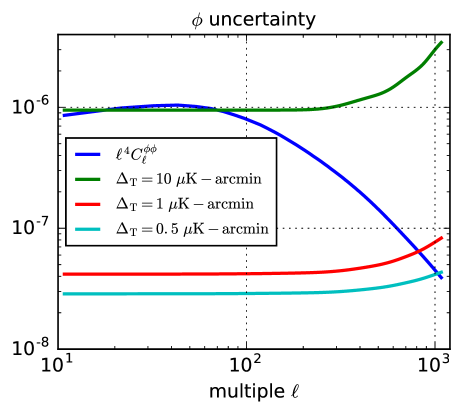
Figure 2: The $\phi(x)$ reconstruction noises for Scenario N ($\Delta_{\rm T}=10$ $\mu$K-arcmin), La ($\Delta_{\rm T}=1$ $\mu$K-arcmin) and Lb ($\Delta_{\rm T}=0.5$ $\mu$K-arcmin) surveys.

We consider a survey strategy consisting of two different surveys of the same area of sky, differing in angular resolution. The main goal of the higher-resolution survey is to allow for a reconstruction of the lensing potential. Such reconstructions benefit from reaching an angular scale comparable to the typical lensing deflection angle of $\sim 2$ arcmin. In contrast, the primordial B-mode signal is on fairly large angular scales of greater than a degree. In principal, one high-resolution survey could be used both for the lensing reconstruction and for sensitivity to the primordial B-mode signal. However, there are advantages to using a survey dedicated to the large-scale signals. These advantages do not appear in the idealized analyses that we perform here, as they are related to systematic error control and foreground cleaning, as we now explain briefly. The large-scale survey can be achieved with a smaller telescope with a simplified optics chain. Having a smaller telescope facilitates boresight rotation, which BICEP2/Keck have used for null tests to bound certain systematic errors. Foreground cleaning is also likely to be more of a challenge at larger angular scales than it is for the smaller-angular scales with the bulk of the lensing information, and serves as a further driver of differences in optimal design for the two surveys. For these reasons a two-survey approach is likely to be a part of the strawman concepts for the CMB Stage-IV instrument soon to emerge from the CMB Stage-IV Concept Definition Taskforce.

In this paper, we simulate three scenarios. We consider a scenario ‘N’ in which the B-mode instrument noise power is larger than the B-mode lensing power, and two scenarios ‘La’ and ‘Lb’ with the opposite situation. The more sensitive scenarios La and Lb are motivated by potential CMB-S4 scenarios. Each scenario consists of two surveys, a high-resolution survey for $\phi$ reconstruction and a low-resolution survey capturing the B-mode signal, covering the same patch of the sky (see Table 2 for the survey configurations in detail). For the high-resolution surveys, the lensing potential reconstruction noise expected from the EB quadratic estimator (Hu, 2001; Hu and Okamoto, 2002; Anderes, 2013) is shown in Figure 2.

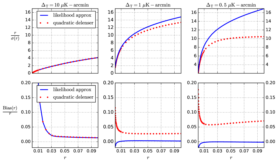
Figure 3: Upper three panels show the detection levels $r/\sigma(r)$ expected from surveys of Scenario N, La, and Lb, and lower three panels show the corresponding bias levels ${\rm Bias(r)}/r$.

IV.2 $r$ Constraints

For each simulated CMB realization, we first reconstruct the lensing potential field from the $\phi$ survey (high resolution survey) using the EB quadratic estimator, then use the reconstructed lensing field $\phi^{\rm est}(x)$ to delense the low resolution polarization maps using the quadratic delenser (Section II) and the modified Gaussian likelihood method (Section III), and finally compare their $r$ constraints from the two delensers.

In Figure 3, we show the detection level $r/\sigma(r)$ and bias level ${\rm Bias}(r)/r$ obtained from the quadratic delenser and from the modified Gaussian likelihood method, where $\sigma(r)$ and ${\rm Bias}(r)$ are the standard error and the average bias of the $500$ best-fit $r$ values (from $500$ CMB realizations), respectively. For Scenario N, both methods obtain similar $r$ detection levels, while the modified Gaussian likelihood method shows its advantages in the Scenario La and Lb. We find that in the regime of low map noise ($\lesssim 1$ $\mu$K-arcmin), the bias of the modified Gaussian likelihood method is appreciably smaller than that of the quadratic delenser (see next subsection for the detailed bias analysis for the quadratic delenser).

For Scenario La with map noise $\Delta_{\rm T}=1$ $\mu$K-arcmin and sky coverage $f_{\rm sky}=2.7\%$, we expect to detect the primordial B-mode signal at $\sim 1\ \sigma$ level for $r=0.001$ and at $\sim 15\ \sigma$ level for $r=0.1$. The lower noise Scenario Lb with map noise $\Delta_{\rm T}=0.5$ $\mu$K-arcmin and the same sky coverage, only marginally increases the detection level, due to the saturation of cosmic variance.

IV.3 Bias Analysis for the Quadratic Delenser

In this subsection, we aim to quantify the bias of the quadratic delenser introduced by ignoring the lensing in E modes and higher order lensing in B modes. For clarity, we use the following notation to denote the connection between lensed and primordial variables

$$\widetilde{E}=E+\delta E_{\text{\rm from E}}+\delta E_{\text{\rm from B}},$$ (27)

$$\widetilde{B}=B+\delta B_{\text{\rm from E}}+\delta B_{\text{\rm from B}},$$

where $\delta X_{\text{\rm from Y}}$ is the lensing in (lensed) $X$ from (primordial) $Y$. In addition, $\delta E_{\text{\rm from B}}$ and $\delta B_{\text{\rm from B}}$ are much smaller than their counterparts $\delta E_{\text{\rm from E}}$ and $\delta B_{\text{\rm from E}}$, so we simply ignore them in this subsection.

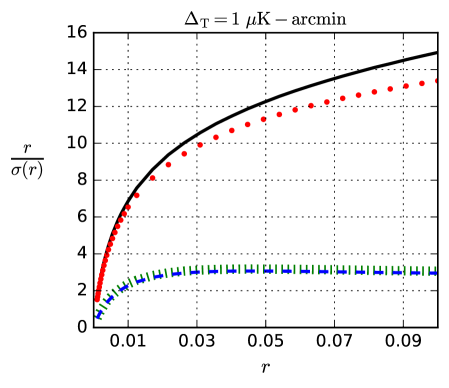
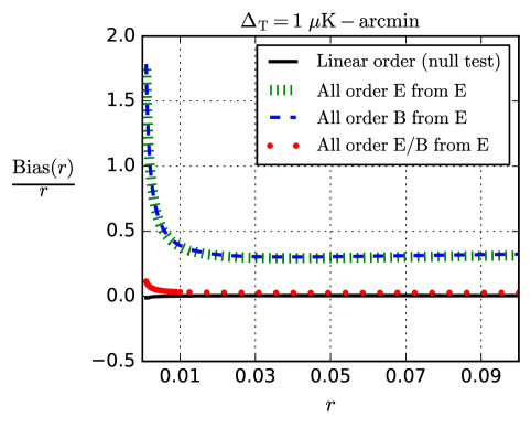
Figure 4: Bias analysis of the quadratic delenser via simulations under different assumptions: (black/solid lines) null test assuming $E^{\rm obs}=E+N^{E}$ and $B^{\rm obs}=B+\delta^{1}B_{\text{\rm from E}}+N^{B}$; (green/bar lines) all order E from E test assuming $E^{\rm obs}=E+\delta E_{\text{\rm from E}}+N^{E}$, $B^{\rm obs}=B+\delta^{1}B_{\text{\rm from E}}+N^{B}$; (blue/dashed lines) all order B from E test assuming $E^{\rm obs}=E+N^{E}$ and $B^{\rm obs}=B+\delta B_{\text{\rm from E}}+N^{B}$; (red/dots) all order E/B from E test assuming $E^{\rm obs}=E+\delta E_{\text{\rm from E}}+N^{E}$ and $B^{\rm obs}=B+\delta B_{\text{\rm from E}}+N^{B}$.

1. First we do a null test. In accordance with the two approximations made in the quadratic delenser (Section II), we completely drop lensing in E modes and only keep linear order lensing in B modes, i.e., we simulate polarization maps assuming $E^{\rm obs}=E+N^{E}$ and $B^{\rm obs}=B+\delta^{1}B_{\text{\rm from E}}+N^{B}$, where $N^{E/B}$ is the E/B map noise, and $\delta^{1}B_{\text{\rm from E}}$ is the linear order lensing in B from E. As expected, we find the quadratic delenser is not biased in this context (Figure 4, black/solid lines).

2. To scrutinize the bias introduced by ignoring lensing in E modes, we keep all order lensing in E modes and linear order lensing in B modes, i.e., we simulate polarization maps assuming $E^{\rm obs}=E+\delta E_{\text{\rm from E}}+N^{E}$ and $B^{\rm obs}=B^{r}+\delta^{1}B_{\text{\rm from E}}+N^{B}$. In this context, the quadratic delenser is highly biased (Figure 4, green/bar lines).

3. In the same way, to test the bias introduced by ignoring high order lensing terms in B modes, we ignore lensing in E modes and keep all order lensing in B modes, i.e., we do simulations assuming $E^{\rm obs}=E+N^{E}$ and $B^{\rm obs}=B+\delta B_{\text{\rm from E}}+N^{B}$. In this context, we also find the quadratic delenser is highly biased. More interestingly, we find that the bias level almost exactly matches that of ignoring lensing in E modes (Figure 4, blue/dashed lines).

4. The final step is to check the interaction between the two bias terms from (iii) and (iv). For this purpose, we keep all order lensing in E modes and all order lensing in B modes, i.e., we simulate polarization maps assuming $E^{\rm obs}=E+\delta E_{\text{\rm from E}}+N^{E}$, and $B^{\rm obs}=B+\delta B_{\text{\rm from E}}+N^{B}$. We find that the two bias contributions cancel to a high precision and therefore the net bias is strongly suppressed (Figure 4, red/dots).

   To make sense of the bias cancellation, we do a simple magnitude analysis. In the quadratic delenser, we delense the B modes via a quadratic template subtraction $B^{\rm res}=B_{\text{\rm from E}}-E^{\rm obs}*\phi^{\rm est}$, and assume a residual power spectrum $C^{BB,{\rm res}}_{\ell}=\langle|\delta^{1}B_{\text{\rm from E}}-E*\phi^{\rm est}|_{\ell}^{2}\rangle$, where $*$ denotes the convolution defined in Equation (2,3), in the $\delta^{1}B_{\text{\rm from E}}$ term we ignore the second (and higher) order lensing in B modes $\delta^{2}B_{\text{\rm from E}}$, and in the $E*\phi$ term we ignore the difference of $E$ and $\widetilde{E}$. Therefore the template subtraction used has an error $\delta^{2}B_{\text{\rm from E}}-\delta^{1}E_{\text{\rm from E}}*\phi$, where both error terms are of the same order $O(E\phi^{2})$ considering that

   $$(\delta^{2}B_{\text{\rm from E}})_{\bm{\ell}}$$ (28)

   $$= -\frac{1}{2}\int\frac{d^{2}{\bm{\ell}_{1}}d^{2}{\bm{\ell}_{2}}}{(2\pi)^{2}}[({\bm{\ell}_{1}}+{\bm{\ell}})\cdot({\bm{\ell}_{1}}+{\bm{\ell}_{2}})]$$

   $$[({\bm{\ell}_{1}}+{\bm{\ell}})\cdot{\bm{\ell}_{2}}]E_{{\bm{\ell}_{1}}+{\bm{\ell}}}\sin(2\varphi_{{\bm{\ell}_{1}}+{\bm{\ell}},{\bm{\ell}}})\phi^{*}_{{\bm{\ell}_{1}}+{\bm{\ell}_{2}}}\phi_{\bm{\ell}_{2}},$$

   and

   $$(\delta^{1}E_{\text{\rm from E}})_{\bm{\ell}}$$ (29)

   $$= \int\frac{d^{2}{\bm{\ell}^{\prime}}}{2\pi}{\bm{\ell}^{\prime}}\cdot({\bm{\ell}^{\prime}}+\bm{\ell})E_{{\bm{\ell}^{\prime}}+\bm{\ell}}\cos(2\varphi_{{\bm{\ell}^{\prime}}+\bm{\ell},\bm{\ell}})\phi^{*}_{\bm{\ell}^{\prime}}.$$

To summarize, in the quadratic delenser,

$$B^{\rm del}_{\bm{\ell}}=B^{r}_{\bm{\ell}}+B^{\rm res}_{\bm{\ell}}+N^{B}_{\bm{\ell}},$$ (30)

we have ignored lensing in E modes and high order lensing in B modes when estimating the residual power spectrum $\langle|B^{\rm res}_{\bm{\ell}}|^{2}\rangle$. We find that each of the two approximation introduces a strong bias in the $r$ estimate, while the two bias contributions cancel to a high precision, and the validity of the quadratic delenser sensitively depends on the cancellation.

According to the above analysis, the bias in the residual power estimate in principle is independent of primordial B-mode signal $B^{r}$, therefore we naively expect a $r$-independent bias ${\rm Bias}(r)$ and therefore a bias level ${\rm Bias}(r)/r$ decaying with growing $r$, which is indeed the behavior we observe for $r\lesssim 0.01$ (Figure 3 and 4). But the bias level does not dies down for even greater $r$, since the $r$ constraints become more sensitive to higher frequency regime where the bias is stronger. Here we give an informal analysis of the bias level behavior. From a single delensed B modes $B^{\rm del}_{\bm{\ell}}$, we can estimate the primordial B-mode power spectrum with root variance $\Delta C_{\bm{\ell}}=C^{BB,r}_{\bm{\ell}}+C^{BB,{\rm res}}_{\bm{\ell}}+N^{BB}_{\bm{\ell}}$, and consequently estimate $r$ with mean value

$$r^{\rm est}_{\bm{\ell}}=\frac{|B^{\rm del}_{\bm{\ell}}|^{2}-C^{BB,{\rm res}}_{\bm{\ell}}-N^{BB}_{\bm{\ell}}}{C^{BB,r=1}_{\bm{\ell}}},$$ (31)

and with root variance $\sigma_{\bm{\ell}}(r)=\Delta C_{\bm{\ell}}/C^{BB,r=1}_{\bm{\ell}}$. These estimators from different modes can be added with inverse-variance weighting $r^{\rm est}=\sum_{\bm{\ell}}W_{\bm{\ell}}r^{\rm est}_{\bm{\ell}}$, where

$$W_{\bm{\ell}}(r)=\frac{\frac{1}{\sigma^{2}_{\bm{\ell}}(r)}}{\sum_{\bm{\ell}}\frac{1}{\sigma^{2}_{\bm{\ell}}(r)}}.$$ (32)

It is straightforward to understand that $W_{\bm{\ell}}(r)$ increases with $r$ for large $|{\bm{\ell}}|$ where $C^{BB,{\rm res}}_{\bm{\ell}}+N^{BB}_{\bm{\ell}}$ dominates $\Delta C_{\bm{\ell}}$, and decreases with $r$ for small $|{\bm{\ell}}|$ where $C^{BB,r}_{\bm{\ell}}$ dominates $\Delta C_{\bm{\ell}}$. In addition, we know that the quadratic delenser is a biased estimator, i.e.,

$$\langle|B^{\rm del}_{\bm{\ell}}|^{2}\rangle=C^{BB,{\rm res}}_{\bm{\ell}}+N^{BB}_{\bm{\ell}}+C^{BB,r}_{\bm{\ell}}+C^{BB,{\rm bias}}_{\bm{\ell}},$$ (33)

and

$$\langle r^{\rm est}_{\bm{\ell}}\rangle=\frac{C^{BB,r}_{\bm{\ell}}+C^{BB,{\rm bias}}_{\bm{\ell}}}{C^{BB,r=1}_{\bm{\ell}}}=r+r^{\rm bias}_{\bm{\ell}},$$ (34)

where $r^{\rm bias}_{\bm{\ell}}$ increases with $|{\bm{\ell}}|$. Therefore, we have $\langle r^{\rm est}\rangle=\sum_{\bm{\ell}}W_{\bm{\ell}}\langle r^{\rm est}_{\bm{\ell}}\rangle=r+\sum_{\bm{\ell}}W_{\bm{\ell}}(r)r^{\rm bias}_{\bm{\ell}}=r+{\rm Bias}(r)$, with ${\rm Bias}(r)$ increasing with $r$. It also explains the increasing bias level ${\rm Bias}(r)$ with decreasing map noise $N^{BB}_{\bm{\ell}}$ (see Figure 3). Note that we do not expect the quadratic delenser to exactly match the inverse-variance weighted estimator described above, but the latter should a good proxy for interpreting the bias behavior.

IV.4 Non-stationary Noise

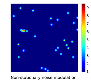
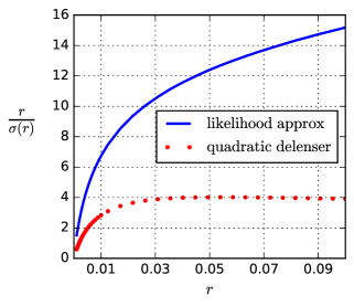
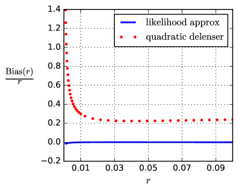
Figure 5: The impact of non-stationary map noise on the $r$ constraints for the Scenario La experiments ($\Delta_{\rm T}=1\ \mu$K-arcmin). Left panel: the non-stationary noise modulation $\sigma(\mathbf{x})$. Middle/Right panel: the detection/bias level of $r$ constraints inferred from the two delensers.

The modified Gaussian likelihood works not only as a correction to the quadratic template subtraction estimator, but also shows its advantage in dealing with realistic experiment complexities, e.g., non-stationary noise and sky cuts. Here we explore an example of non-stationary noise with pixel dependent noise, i.e., $\left<n(\mathbf{x})n(\mathbf{y})\right>=\sigma^{2}(\mathbf{x})\Delta_{\rm P}^{2}\delta_{D}(\mathbf{x}-\mathbf{y})$, with $\Delta_{\rm P}=\sqrt{2}\ \Delta_{\rm T}=\sqrt{2}\ \mu$K-arcmin, and $\sigma(\mathbf{x})$ a pixel-dependent modulation (Figure 5). We expect the likelihood based estimator to work robustly in the presence of non-stationary noise, as long as we take the pixel dependent noise into account when calculating the covariance matrix of noise (see Appendix B). But the non-stationary noise becomes troublesome for the quadratic delenser in Fourier space.

Applying the two estimators on simulations with non-stationary noise, we find that the modified Gaussian likelihood method works as well as in the case of stationary noise, while the quadratic delenser is significantly biased (Figure 5).

V Summary and Conclusions

Delensing is a crucial part for future CMB experiments aiming to detect a primordial B-mode signal. Up to linear order, one can effectively delense observed B-modes by utilizing a quadratic combination of observed E-modes and an estimate of the lensing potential. This is the underlying idea of the quadratic delenser. However, in the regime of small map noise, the lensing in E modes, and higher order lensing in B modes ignored by the quadratic delenser, significantly bias the $r$ constraint. We investigated the bias induced by each of the two approximations via simulations, finding that each of two approximations induce a large bias, while the two bias terms partly cancel and therefore the net bias is moderately suppressed. The validity of the quadratic delenser sensitively depends on the cancellation.

Alternatively, a full-scale likelihood analysis of the tensor-to-scalar ratio $r$ can, in principle, optimally account for all the $r$ information in the CMB observations and remedy possible bias problems. Unfortunately, a full likelihood analysis requires computation resources beyond what is available in the near future. In this paper, we presented a modified Gaussian likelihood method. This method consists of two parts, covariance decomposition and data compression. In the first part, we decomposed the covariance matrix in the form of $\Sigma_{r}=\Sigma^{\rm en}+r\Sigma^{\rm b}$, which allows us to compute the covariance matrix $\Sigma_{r}$, as a function of $r$, at the computational cost of a single covariance matrix evaluation. In the second part, we compressed the data size by keeping only $s\sim 500$ high signal-to-noise modes, say the large-scale quadratic delensed B modes. We obtained these B modes from polarization data $d$ via a projection matrix $v$, $(^{0}B^{\rm del}_{\bm{\ell}})_{s}=(v^{\intercal})_{s\times 2p}d_{2p}$, and applied the likelihood analysis on the projected data vector. This method can be naturally extended to incorporate higher frequency modes.

Finally, we applied the quadratic delenser and the modified Gaussian likelihood method on simulated CMB observations mimicking experiments of Scenario N, La, and Lb, and compare the resulting $r$ constraints. We found that, the two methods have similar performance in constraining $r$ for Scenario N, while the quadratic delenser does not perform as well for the lower-noise Scenario La and Lb due to a strong $r$ constraint bias in the regime of low map noise. For Scenario La, we expected to detect the primordial B-mode signal at $\sim 1\sigma$ level for $r=0.001$, and at $\sim 15\sigma$ level for $r=0.1$, from the modified Gaussian likelihood method. For Scenario Lb with even lower map noise and the same sky coverage, the detection level only marginally increases due to the saturation of cosmic variance. Therefore it would be valuable to optimize the survey configurations (${\Delta_{\rm T},f_{\rm sky}}$) for the coming CMB experiments given a fixed amount of survey time (CMB-S4 Collaboration, 2016).

We also explored the impact of realistic experiment complexities: in the presence of non-stationary noise, the modified Gaussian likelihood method also works robustly as long as we slightly modify the noise covariance matrix to take into account the pixel dependent noise.

Appendix A Signal Covariance Matrix

There are eight different terms in the map covariance matrix $\Sigma_{r}$: $\{\tilde{\Sigma}^{SE,SE},\tilde{\Sigma}^{CE,SE},\tilde{\Sigma}^{CE,CE}\}$, $\{\tilde{\Sigma}^{SB,SB},\tilde{\Sigma}^{CB,SB},\tilde{\Sigma}^{CB,CB}\}$, and $\{\Sigma^{NQ,NQ},\Sigma^{NU,NU}\}$ (see Equations (16)). In this subsection, we show how the marginalization over uncertainty in the $\phi$ estimate is done for the six lensed signal terms, and leave the two noise terms to the next subsection. Take $\tilde{\Sigma}^{XX}(X=SE)$ as an example,

$$\left<\tilde{\Sigma}^{XX}_{r,\phi}\right>_{n\phi} =\left<\widetilde{X}(\mathbf{x})\widetilde{X}(\mathbf{y})\right>_{n\phi}$$ (35)

$$=\left<X(x+\nabla\mu\phi(\mathbf{x})+\nabla n\phi(\mathbf{x}))X(\mathbf{y}+\nabla\mu\phi(\mathbf{y})+\nabla n\phi(\mathbf{y}))\right>_{n\phi}$$

$$=\int\frac{d^{2}\bm{\ell}}{(2\pi)^{2}}e^{i\bm{\ell}\cdot(\mathbf{x}-\mathbf{y}+\nabla\mu\phi(\mathbf{x})-\nabla\mu\phi(\mathbf{y}))}C_{\ell}^{XX}\left<e^{i\bm{\ell}\cdot(\nabla n\phi(\mathbf{x})-\nabla n\phi(\mathbf{y}))}\right>_{n\phi}$$

$$=\int\frac{d^{2}\bm{\ell}}{(2\pi)^{2}}e^{i\bm{\ell}\cdot(\mathbf{x}-\mathbf{y}+\nabla\mu\phi(\mathbf{x})-\nabla\mu\phi(\mathbf{y}))}C_{\ell}^{XX}\exp\{-\bm{\ell}\cdot\left[\Sigma^{n\phi}(0)-\Sigma^{n\phi}(\mathbf{x}-\mathbf{y})\right]\cdot\bm{\ell}\}$$

$$\simeq\int\frac{d^{2}\bm{\ell}}{(2\pi)^{2}}e^{i\bm{\ell}\cdot(\mathbf{x}-\mathbf{y}+\nabla\mu\phi(\mathbf{x})-\nabla\mu\phi(\mathbf{y}))}C_{\ell}^{XX}\left(1-\bm{\ell}\cdot\left[\Sigma^{n\phi}(0)-\Sigma^{n\phi}(\mathbf{x}-\mathbf{y})\right]\cdot\bm{\ell}\right)$$

$$=\int\frac{d^{2}\bm{\ell}}{(2\pi)^{2}}e^{i\bm{\ell}\cdot(\mathbf{x}-\mathbf{y}+\nabla\mu\phi(\mathbf{x})-\nabla\mu\phi(\mathbf{y}))}C_{\ell}^{XX}$$

$$-\sum_{p,q=1}^{2}\left[\Sigma^{n\phi}(0)-\Sigma^{n\phi}(\mathbf{x}-\mathbf{y})\right]_{p,q}\int\frac{d^{2}\bm{\ell}}{(2\pi)^{2}}\ell_{p}\ell_{q}e^{i\bm{\ell}\cdot(\mathbf{x}-\mathbf{y}+\nabla\mu\phi(\mathbf{x})-\nabla\mu\phi(\mathbf{y}))}C_{\ell}^{XX}$$

$$={\rm Cov}(X(\mathbf{w}),X(0))+\sum_{p,q=1}^{2}\left[\Sigma^{n\phi}(0)-\Sigma^{n\phi}(\mathbf{x}-\mathbf{y})\right]_{p,q}\partial_{p,q}{\rm Cov}(X(\mathbf{w}),X(0))$$

where we have used cumulant expansion at the 4th equal sign, $\left[\Sigma^{n\phi}(\mathbf{x}-\mathbf{y})\right]_{p,q}$ is the covariance of $\nabla(n\phi)$, i.e.,

$$\left[\Sigma^{n\phi}(\mathbf{x}-\mathbf{y})\right]_{p,q} =\left<\nabla_{p}n\phi(\mathbf{x})\nabla_{q}n\phi(\mathbf{y})\right>_{n\phi}=\int\frac{d^{2}\bm{\ell}}{(2\pi)^{2}}\ell_{p}\ell_{q}e^{i\bm{\ell}\cdot(\mathbf{x}-\mathbf{y})}N_{\ell}^{\phi\phi},$$ (36)

and ${\rm Cov}(X(\mathbf{w}),X(0))$ is the covariance of $X$ at separation $\mathbf{w}=\mathbf{x}-\mathbf{y}+\nabla\mu\phi(\mathbf{x})-\nabla\mu\phi(\mathbf{y})$,

$${\rm Cov}(X(\mathbf{w}),X(0))=\int\frac{d^{2}\bm{\ell}}{(2\pi)^{2}}e^{i\bm{\ell}\cdot\mathbf{w}}C_{\ell}^{XX}.$$ (37)

The above two dimensional integrals (Equations (36-37)) can be simplified as one dimensional integrals as follows. Take Equation (37) as an example,

$${\rm Cov}\left(X(\mathbf{w}),X(0)\right) =4\partial_{1}^{2}\partial_{2}^{2}\int\frac{d^{2}\bm{\ell}}{(2\pi)^{2}}e^{i\bm{\ell}\cdot\mathbf{w}}C_{\ell}^{\mathcal{E}\mathcal{E}}$$ (38)

$$\equiv 4\partial_{1}^{2}\partial_{2}^{2}K^{\mathcal{E}}(w),$$

where we have used $C_{\ell}^{XX}=4\ell_{1}^{2}\ell_{2}^{2}(C_{\ell}^{EE}/\ell^{4})$ and defined $C_{\ell}^{\mathcal{E}\mathcal{E}}\equiv C_{\ell}^{EE}/\ell^{4}$. Exploiting the integral representation of Bessel functions, we rewrite $K^{\mathcal{E}}(\mathbf{w})$ as a one dimensional integral

$$K^{\mathcal{E}}(\mathbf{w}) =\int\frac{d^{2}\bm{\ell}}{(2\pi)^{2}}e^{i\bm{\ell}\cdot\mathbf{w}}C_{\ell}^{\mathcal{E}\mathcal{E}}$$ (39)

$$=\frac{1}{2\pi}\int J_{0}\left(\ell w\right)C_{\ell}^{\mathcal{E}\mathcal{E}}\ell d\ell,$$

which has no angular dependence. For derivative calculation, we define $\hat{K}(w^{2})\equiv K^{\mathcal{E}}(\mathbf{w})$, then

$$\partial_{1}^{2}\partial_{2}^{2}K^{\mathcal{E}}(\mathbf{w})=\partial_{1}^{2}\partial_{2}^{2}\hat{K}(w^{2})$$ (40)

$$=16w_{1}^{2}w_{2}^{2}\ \hat{K}^{(4)}(w^{2})$$

$$+8(w_{1}^{2}+w_{2}^{2})\ \hat{K}^{(3)}(w^{2})+4\hat{K}^{(2)}(w^{2}).$$

Using the property

$$\frac{d}{dz}z^{-s}J_{s}(z)=-z^{-s}J_{s+1}(z),$$ (41)

the $n$-th order derivative $\hat{K}^{(n)}$ is explicitly expressed as

$$\hat{K}^{(n)}(w^{2})=\frac{1}{2\pi}\int\left(-\frac{\ell}{2w}\right)^{n}J_{n}(\ell w)\ell d\ell.$$ (42)

Collecting Equations (38, 40, 42), ${\rm Cov}\left(X(\mathbf{w}),X(0)\right)$ is decomposed into a few one dimensional integrals. The calculation of $\partial_{p,q}{\rm Cov}\left(X(\mathbf{w}),X(0)\right)$ and $\left[\Sigma^{n\phi}(\mathbf{x}-\mathbf{y})\right]_{p,q}$ is conducted in the same way. For other lensed terms, the above formulas apply similarly.

Appendix B Noise Covariance Matrix

In Section A, we completely ignore the consequence of the finite beam size in the signal covariance evaluation, since the signal suppression by the beam convolution can be interpreted as the noise enhancement by the beam deconvolution. For noise field $n(\mathbf{x})$, we denote the deconvolved noise field as $X(\mathbf{x})=\varphi^{-1}_{x}[n(\mathbf{x})]$, with

$$\varphi^{-1}_{x}[n(\mathbf{x})] =\int\frac{d^{2}\bm{\ell}}{2\pi}e^{i\bm{\ell}\cdot\mathbf{x}}\frac{n_{\bm{\ell}}}{\varphi_{\bm{\ell}}}$$ (43)

$$=\int\frac{d^{2}\bm{\ell}}{2\pi}\frac{d^{2}\mathbf{x}^{\prime}}{2\pi}e^{i\bm{\ell}\cdot(\mathbf{x}-\mathbf{x}^{\prime})}\frac{n(\mathbf{x}^{\prime})}{\varphi_{\bm{\ell}}},$$

where for Gaussian beam profile $\varphi(\mathbf{x})=\frac{1}{2\pi\sigma_{b}^{2}}\exp\left(-\frac{\mathbf{x}^{2}}{2\sigma_{b}^{2}}\right)$, $\varphi_{\bm{\ell}}=\exp\left(-\frac{l^{2}\sigma_{b}^{2}}{2}\right)$, and $\sigma_{b}^{2}=\theta^{2}_{\rm FWHM}/(8\ln 2)$. Then

$$\Sigma^{XX}=\left<X(\mathbf{x})X(\mathbf{y})\right> =\int\frac{d^{2}\bm{\ell}}{2\pi}\frac{d^{2}\mathbf{x}^{\prime}}{2\pi}\frac{d^{2}\mathbf{k}}{2\pi}\frac{d^{2}\mathbf{y}^{\prime}}{2\pi}e^{i\bm{\ell}\cdot(\mathbf{x}-\mathbf{x}^{\prime})}e^{i\mathbf{k}\cdot(\mathbf{y}-\mathbf{y}^{\prime})}\frac{1}{\varphi_{\bm{\ell}}\varphi_{\mathbf{k}}}\left<n(\mathbf{x}^{\prime})n(\mathbf{y}^{\prime})\right>,$$ (44)

For simple white noise $\left<n(\mathbf{x})n(\mathbf{y})\right>=\Delta_{\rm P}^{2}\delta_{D}(\mathbf{x}-\mathbf{y})$, we have

$$\left<X(\mathbf{x})X(\mathbf{y})\right> =\int\frac{d^{2}\bm{\ell}}{(2\pi)^{2}}e^{i\bm{\ell}\cdot(\mathbf{x}-\mathbf{y})}\frac{\Delta_{\rm P}^{2}}{\varphi_{\bm{\ell}}\varphi_{-\bm{\ell}}}=\Delta_{\rm P}^{2}\int\frac{d^{2}\bm{\ell}}{(2\pi)^{2}}e^{i\bm{\ell}\cdot(\mathbf{x}-\mathbf{y})}\ e^{\ell^{2}\sigma_{b}^{2}},$$ (45)

where $\Delta_{\rm P}$ is polarization noise and we usually take $\Delta_{\rm P}=\sqrt{2}\Delta_{\rm T}$. For more realistic non-stationary noise $\left<n(\mathbf{x})n(\mathbf{y})\right>=\sigma^{2}(\mathbf{x})\Delta_{\rm P}^{2}\delta_{D}(\mathbf{x}-\mathbf{y})$, the covariance matrix of the deconvolved noise field $X(\mathbf{x})$ is written as

$$\left<X(\mathbf{x})X(\mathbf{y})\right> =\left<\varphi_{x}^{-1}[n(\mathbf{x})]\ \varphi_{y}^{-1}[n(\mathbf{y})]\right>$$ (46)

$$=\left<\varphi_{x}^{-1}[n(\mathbf{x})]\ \int\frac{d^{2}\bm{\ell}}{2\pi}\frac{d^{2}\mathbf{y}^{\prime}}{2\pi}e^{i\bm{\ell}\cdot(\mathbf{y}-\mathbf{y}^{\prime})}\frac{n(\mathbf{y}^{\prime})}{\varphi_{\bm{\ell}}}\right>$$

$$=\varphi_{x}^{-1}\left[\int\frac{d^{2}\bm{\ell}}{2\pi}\frac{d^{2}\mathbf{y}^{\prime}}{2\pi}e^{i\bm{\ell}\cdot(\mathbf{y}-\mathbf{y}^{\prime})}\frac{1}{\varphi_{\bm{\ell}}}\left<n(\mathbf{x})n(\mathbf{y}^{\prime})\right>\right]$$

$$=\varphi_{x}^{-1}\left[\sigma^{2}(\mathbf{x})\Delta_{\rm P}^{2}\int\frac{d^{2}\bm{\ell}}{(2\pi)^{2}}e^{i\bm{\ell}\cdot(\mathbf{y}-\mathbf{x})}e^{\frac{\ell^{2}\sigma_{b}^{2}}{2}}\right]$$

where we have exchanged the order of deconvolution and ensemble average at the 3rd equal sign, since deconvolution is a linear operator.

$$\left<X(\mathbf{x})X(\mathbf{y})\right> =\Delta_{\rm P}^{2}\int\frac{d^{2}\bm{\ell}}{(2\pi)^{2}}\frac{d^{2}\mathbf{k}}{2\pi}e^{i\bm{\ell}\cdot\mathbf{x}}e^{i\mathbf{k}\cdot\mathbf{y}}\varphi_{\bm{\ell}}\varphi_{\mathbf{k}}\left[\int\frac{d^{2}\mathbf{x}^{\prime}}{2\pi}e^{-i(\bm{\ell}+\mathbf{k})\cdot\mathbf{x}^{\prime}}\delta^{2}(\mathbf{x}^{\prime})\right]$$ (47)

$$=\Delta_{\rm P}^{2}\int\frac{d^{2}\bm{\ell}}{(2\pi)^{2}}\frac{d^{2}\mathbf{k}}{2\pi}e^{i\bm{\ell}\cdot\mathbf{x}}e^{i\mathbf{k}\cdot\mathbf{y}}\varphi_{\bm{\ell}}\varphi_{\mathbf{k}}\ (\delta^{2})_{\bm{\ell}+\mathbf{k}}$$

$$=\Delta_{\rm P}^{2}\int\frac{d^{2}\bm{\ell}}{(2\pi)^{2}}e^{i\bm{\ell}\cdot\mathbf{x}}\varphi_{\bm{\ell}}\int\frac{d^{2}\mathbf{k}}{2\pi}e^{i\mathbf{k}\cdot\mathbf{y}}\varphi_{\mathbf{k}}\ (\delta^{2})_{\bm{\ell}+\mathbf{k}}$$

Appendix C Inverse of Covariance Matrix

The inverse covariance matrix $\Sigma_{r}^{-1}$ evaluation is the key to the $r$ likelihood in Equation (10). To avoid repeating the similar computation for every different $r$, we can single out the $r$ dependence rewriting the covariance matrix in the form $\Sigma_{r}=\Sigma^{\rm en}+r\Sigma^{\rm b}$, where

$$\Sigma^{\rm en} =\left(\begin{tabular}[]{cc}$\tilde{\Sigma}^{CE,CE}+\Sigma^{NQ,NQ}$&$\tilde{\Sigma}^{CE,SE}$\\ $\tilde{\Sigma}^{CE,SE}$&$\tilde{\Sigma}^{SE,SE}+\Sigma^{NU,NU}$\end{tabular}\right),$$

$$\Sigma^{\rm b} =\left(\begin{tabular}[]{cc}$\tilde{\Sigma}^{SB^{0},SB^{0}}$&$\tilde{\Sigma}^{CB^{0},SB^{0}}$\\ $\tilde{\Sigma}^{CB^{0},SB^{0}}$&$\tilde{\Sigma}^{CB^{0},CB^{0}}$\end{tabular}\right).$$

Both $\Sigma^{\rm en}$ and $\Sigma^{\rm b}$ are symmetric and positive definite. We first decompose $\Sigma^{\rm b}$ as $\Sigma^{\rm b}=V\Lambda V^{\intercal}$, with $\Lambda$ being a diagonal matrix composed of its eigenvalues, and $V$ being a matrix composed of its eigenvectors. Now we do a little manipulation to the covariance matrix

$$\Sigma_{r} =\Sigma^{\rm en}+rV\Lambda V^{\intercal}$$ (48)

$$=V\sqrt{\Lambda}\left(\sqrt{\Lambda^{-1}}V^{\intercal}\Sigma^{\rm en}V\sqrt{\Lambda^{-1}}+rI\right)\sqrt{\Lambda}V^{\intercal},$$

where we have used the orthogonality $V^{\intercal}=V^{-1}$. One more eigendecomposition, $\sqrt{\Lambda^{-1}}V^{\intercal}\Sigma^{\rm en}V\sqrt{\Lambda^{-1}}=\hat{V}\hat{\Lambda}\hat{V}^{\intercal}$, enables us further transform $\Sigma_{r}$ as

$$\Sigma_{r} =V\sqrt{\Lambda}\hat{V}\left(\hat{\Lambda}+rI\right)\hat{V}^{\intercal}\sqrt{\Lambda}V^{\intercal}$$ (49)

$$=V\sqrt{\Lambda}\hat{V}\left(\hat{\Lambda}+rI\right)(V\sqrt{\Lambda}\hat{V})^{\intercal}.$$

Here we can obtain the inverse matrix $\Sigma_{r}^{-1}$ at little cost, using the orthogonality of $V$ and $\hat{V}$. And more beautifully, all the matrices $V,\Lambda$ and $\hat{V},\hat{\Lambda}$ have no $r$ dependence, hence we obtain the inverse covariance matrix as a function of $r$ at the same computation cost of a single inverse matrix computation.