Universality in Systems with Power-Law Memory and Fractional Dynamics

1 Introduction

Sir Robert M. May’s paper “Simple mathematical models with very complicated dynamics” published 41 years ago in “Nature” May is one of the most cited papers - 3057 citations are registered by the Web of Science at the moment I am writing this sentence. In this review the author, using the logistic map as an example, described the universal behavior typical for all nonlinear systems: transition to chaos through the period-doubling cascade of bifurcations. The main applications considered by the author are the biological (even the variable used in the text was treated as “the population”), economic, and social sciences. The major steps in the development of the notion of universality in non-linear dynamics are gathered in the reprinted selection of papers compiled by Predrag Cvitanovic Cvi , and applications of universality encompass all areas of science.

The logistic map is a very simple discrete non-linear model of dynamical evolution. More realistic models of biological, economic, and social systems are more complicated. One of the features, not reflected in this equation but which is present in all the abovementioned systems, is memory. Evolution of any social or biological system depends not only on the current state of a system but on the whole history of its development. In majority of cases this memory obeys the power law. There are many reviews on power-law distributions and memory in various social systems (see, e.g., Mach ). In papers Adaptation3 ; Adaptation4 ; Adaptation2 ; Adaptation5 ; Adaptation1 ; Adaptation6 the power-law adaptation has been used to describe the dynamics of biological systems. The impotence and origin of the memory in biological systems can be related to the presence of memory at the level of individual cells: it has been shown recently that processing of external stimuli by individual neurons can be described by fractional differentiation Neuron3 ; Neuron4 ; Neuron5 . The orders of fractional derivatives $\alpha$ derived for different types of neurons fall within the interval [0,1], which implies power-law memory $\sim t^{\beta}$ with power $\beta=\alpha-1$, $\beta\in[-1,0]$. For neocortical pyramidal neurons the order of the fractional derivative is quite small: $\alpha\approx 0.15$. At the level of a human individual as a whole the power law appears in the study of human memory: forgetting - the accuracy on memory tasks decays as a power law with $\beta\in[-1,0]$ Kahana ; Rubin ; Wixted1 ; Wixted2 ; Adaptation1 ; learning - the reduction in reaction times that comes with practice is a power function of the number of training trials Anderson . Power-law memory appears in the study of the human organ tissues due to their viscoelastic properties (see, e.g., references in Chaos2015 ). This leads to their description by fractional differential equations with time fractional derivatives which implies the power-law memory. In most of the biological systems with the power-law behavior the power $\beta$ is between -1 and 1 ($0<\alpha<2$).

It is much easier to investigate general properties of discrete systems with power-law memory than properties of integro-differential equations with power-law kernel. In section 2 we review different ways to introduce or derive maps with power-law memory and their relation to fractional differential/difference equations. Periodic sinks and their stability (the stability of fixed points and asymptotic period two ($T=2$) sinks) in fractional systems are discussed in section 3. In section 4 we consider various forms (non-linearity parameter, two-dimensional, and memory parameter) of bifurcation diagrams and transition to chaos in discrete fractional systems. In the conclusion we discuss perspectives and application of the research on the universality in fractional systems.

2 Maps with power-law memory and fractional maps

In this section we consider various ways to introduce maps with power-law memory and fractional maps following ME2 ; ME3 ; ME4 ; ME6 ; ME7 ; ME8 ; ME9 ; Chaos2015 ; ME1 ; ME5 ; T2009a ; T2009b ; T2 ; T1 ; FallC ; Fall .

In the following we will use two definitions of fractional derivatives. They are based on the fractional integral introduced by Liouville, which is a generalization of the Cauchy formula for the n-fold integral

$${}_{a}I^{p}_{t}x(t)=\frac{1}{\Gamma(p)}\int^{t}_{a}\frac{x(\tau)d\tau}{(t-\tau)^{1-p}}~{},$$ (1)

where $p$ is a real number, $\Gamma()$ is the gamma function and we will assume $a=0$.

The first one is the left-sided Riemann-Liouville fractional derivative ${}_{0}D^{\alpha}_{t}x(t)$ defined for $t>0$ KST ; Podlubny ; SKM as

$${}_{0}D^{\alpha}_{t}x(t)=D^{n}_{t}\ {}_{0}I^{n-\alpha}_{t}x(t)=\frac{1}{\Gamma(n-\alpha)}\frac{d^{n}}{dt^{n}}\int^{t}_{0}\frac{x(\tau)d\tau}{(t-\tau)^{\alpha-n+1}}~{},$$ (2)

where $n-1\leq\alpha<n$, $n\in\mathbb{Z}$, $D^{n}_{t}=d^{n}/dt^{n}$.

The second one is the left-sided Caputo derivative, in which the order of integration and differentiation in Eq. (2) is switched KST

$${}_{0}^{C}D^{\alpha}_{t}x(t)=_{0}I^{n-\alpha}_{t}\ D^{n}_{t}x(t)=\frac{1}{\Gamma(n-\alpha)}\int^{t}_{0}\frac{D^{n}_{\tau}x(\tau)d\tau}{(t-\tau)^{\alpha-n+1}}\quad(n-1<\alpha\leq n).$$ (3)

2.1 Direct introduction of maps with power-law memory

The direct way to introduce maps with power-law memory is to define them as convolutions according to the formula (see Chaos2015 ; StanislavskyMaps )

$$x_{n}=\sum^{n-1}_{k=0}(n-k)^{\alpha-1}G_{K}(x_{k},h),$$ (4)

where $K$ is a parameter and $h$ is a constant time step between time instants $t_{n}$ and $t_{n+1}$. For a physical interpretation of this formula we consider a system which state is defined by the variable $x$ and evolution by the function $G_{K}(x)$. The value of the state variable at the time $t_{n}$ is a weighted total of the functions $G_{K}(x_{k})$ from the values of this variable at past time instants $t_{k}$, $0<k<n$, $t_{k}=kh$. The weights are the times between time instants $t_{n}$ and $t_{k}$ to the fractional power $\alpha-1$.

The more general form of this map considered in Chaos2015 ; StanislavskyMaps (see, e.g., Eq. (73) from Chaos2015 ) is

$$x_{n}=\sum^{\lceil\alpha\rceil-1}_{k=1}\frac{c_{k}}{\Gamma(\alpha-k+1)}(nh)^{\alpha-k}+\sum^{n-1}_{k=0}(n-k)^{\alpha-1}G_{K}(x_{k},h),$$ (5)

where $\alpha\in\mathbb{R}$. If we assume

$$G_{K}(x,h)=\frac{1}{\Gamma(\alpha)}h^{\alpha}G_{K}(x),$$ (6)

where $G_{K}(x)$ is continuous, and

$$x=x(t),\ \ x_{k}=x(t_{k}),\ \ t_{k}=a+kh,\ \ nh=t-a$$ (7)

for $0\leq k\leq n$, then this equation can be written as

$$x_{n}=\sum^{\lceil\alpha\rceil-1}_{k=1}\frac{c_{k}}{\Gamma(\alpha-k+1)}(nh)^{\alpha-k}+\frac{h^{\alpha}}{\Gamma({\alpha})}\sum^{n-1}_{k=0}(n-k)^{\alpha-1}G_{K}(x_{k}).$$ (8)

Eq.  (8) in the limit $h\rightarrow 0+$ will yield the Volterra integral equation of the second kind

$$x(t)=\sum^{\lceil\alpha\rceil-1}_{k=1}\frac{c_{k}}{\Gamma(\alpha-k+1)}(t-a)^{\alpha-k}+\frac{1}{\Gamma(\alpha)}\int^{t}_{a}\frac{G_{K}(\tau,x(\tau))d\tau}{(t-\tau)^{1-\alpha}},\ \ \ (t>a).$$ (9)

This equation is equivalent to the fractional differential equation with the Riemann-Liouville or Gr$\ddot{u}$nvald-Letnikov fractional derivative Chaos2015 ; KBT1 ; KBT2

$${}_{a}^{RL/GL}D^{\alpha}_{t}x(t)=G_{k}(t,x(t)),\ \ 0<\alpha$$ (10)

with the initial conditions

$$(_{a}^{RL/GL}D^{\alpha-k}_{t}x)(a+)=c_{k},\ \ \ k=1,2,...,\lceil\alpha\rceil.$$ (11)

For $\alpha\not\in\mathbb{N}$ we assume $c_{\lceil\alpha\rceil}=0$, which corresponds to a finite value of $x(a)$.

2.2 Universal map with power-law memory from fractional differential equations of systems with periodic delta-function kicks

The universal map and its particular form, the standard map, play an important role in the study of regular dynamical systems. Their fractional generalizations can be obtained in a way similar to the way in which the regular universal map is derived from the differential equation of a periodically (with the period $h$) kicked system in regular dynamics (see, e.g., ZasBook ). The two-dimensional fractional universal map obtained from the differential equation of the order $1<\alpha\leq 2$ was introduced in T1 , extended to any real $\alpha>1$ in T2009a ; T2009b ; T2 , and then to any $\alpha\geq 0$ in ME3 ; ME4 ; ME7 .

To derive the equations of the fractional universal map, which we’ll call the universal $\alpha$-family of maps ($\alpha$-FM) for $\alpha\geq 0$, we start with the differential equation

$$\frac{d^{\alpha}x}{dt^{\alpha}}+G_{K}(x(t-\Delta h))\sum^{\infty}_{k=-\infty}\delta\Bigl{(}\frac{t}{h}-(k+\varepsilon)\Bigr{)}=0,$$ (12)

where $\varepsilon>\Delta>0$, $\alpha\in\mathbb{R}$, $\alpha>0$, and consider it as $\varepsilon\rightarrow 0$. The initial conditions should correspond to the type of fractional derivative used in Eq. (12). The case $\alpha=2$, $\Delta=0$, and $G_{K}(x)=KG(x)$ corresponds to the equation whose integration yields the regular universal map.

Integration of Eq. (12) with the Riemann-Liouville fractional derivative ${}_{0}D^{\alpha}_{t}x(t)$ and the initial conditions

$$(_{0}D^{\alpha-k}_{t}x)(0+)=c_{k},$$ (13)

where $k=1,...,N$ and $N=\lceil\alpha\rceil$, yields the Riemann-Liouville universal $\alpha$-FM

$$x_{n+1}=\sum^{N}_{k=1}\frac{c_{k}}{\Gamma(\alpha-k+1)}h^{\alpha-k}(n+1)^{\alpha-k}-\frac{h^{\alpha}}{\Gamma(\alpha)}\sum^{n}_{k=0}G_{K}(x_{k})(n-k+1)^{\alpha-1}.$$ (14)

As in the Sec. 2.1, for $\alpha\not\in\mathbb{N}$ boundedness of $x(t)$ at $t=0$ requires $c_{N}=0$ and $x(0)=0$ (see KST ; Podlubny ; SKM ). Obtained in Sec. 2.1 Eq. (8) is identical to Eq. (14).

Integration of Eq. (12) with the Caputo fractional derivative ${}_{0}^{C}D^{\alpha}_{t}x(t)$ and the initial conditions $(D^{k}_{t}x)(0+)=b_{k}$, $k=0,...,N-1$, yields the Caputo universal $\alpha$-FM

$$x_{n+1}=\sum^{N-1}_{k=0}\frac{b_{k}}{k!}h^{k}(n+1)^{k}-\frac{h^{\alpha}}{\Gamma(\alpha)}\sum^{n}_{k=0}G_{K}(x_{k})(n-k+1)^{\alpha-1}.$$ (15)

Later in this paper we’ll refer to the maps Eqs. (8) and (14), the RL universal $\alpha$-FM, as the Riemann-Liouville universal map with power-law memory or the Riemann-Liouville universal fractional map; we’ll call the Caputo universal $\alpha$-FM, Eq. (15), the Caputo universal map with power-law memory or the Caputo universal fractional map.

In the case of integer $\alpha$ the universal map converges to

$$x_{n}=0\ \ {\rm for}\ \ \alpha=0\ \ {\rm and}\ \ x_{n+1}=x_{n}-hG_{K}(x_{n})\ \ {\rm for}\ \ \alpha=1,$$ (16)

and for $\alpha=N=2$ with $p_{n+1}=(x_{n+1}-x_{n})/h$

$$\begin{array}[]{c}\left\{\begin{array}[]{lll}p_{n+1}=p_{n}-hG_{K}(x_{n}),\ \ n\geq 0,\\ x_{n+1}=x_{n}+hp_{n+1},\ \ n\geq 0.\end{array}\right.\end{array}$$ (17)

N-dimensional, with $N\geq 2$, universal maps are investigated in ME4 , where it is shown that they are volume preserving.

2.3 Universal fractional difference map

The fractional sum ($\alpha>0$)/difference ($\alpha<0$) operator introduced by Miller and Ross in MR

$${}_{a}\Delta^{-\alpha}_{t}f(t)=\frac{1}{\Gamma(\alpha)}\sum^{t-\alpha}_{s=a}(t-s-1)^{(\alpha-1)}f(s)$$ (18)

can be considered as a fractional generalization of the $n$-fold summation formula ME9 ; GZ

$${}_{a}\Delta^{-n}_{t}f(t)=\frac{1}{(n-1)!}\sum^{t-n}_{s=a}(t-s-1)^{(n-1)}f(s)=\sum^{t-n}_{s^{0}=a}\sum^{s^{0}}_{s^{1}=a}...\sum^{s^{n-2}}_{s^{n-1}=a}f(s^{n-1}),$$ (19)

where $n\in\mathbb{N}$ and $s^{i}$, $i=0,1,...n-1$, are the summation variables. In Eq. (18) $f$ is defined on $\mathbb{N}_{a}$ and ${}_{a}\Delta^{-\alpha}_{t}$ on $\mathbb{N}_{a+\alpha}$, where $\mathbb{N}_{t}=\{t,t+1,t+2,...\}$. The falling factorial $t^{(\alpha)}$ is defined as

$$t^{(\alpha)}=\frac{\Gamma(t+1)}{\Gamma(t+1-\alpha)},\ \ t\neq-1,-2,-3,...$$ (20)

and is asymptotically a power function:

$$\lim_{t\rightarrow\infty}\frac{\Gamma(t+1)}{\Gamma(t+1-\alpha)t^{\alpha}}=1,\ \ \ \alpha\in\mathbb{R}.$$ (21)

For $\alpha>0$ and $m-1<\alpha<m$ the fractional (left) Riemann-Liouville difference operator is defined (see Atici1 ; Atici2 ) as

$${}_{a}\Delta^{\alpha}_{t}x(t)=\Delta^{m}_{a}\Delta^{-(m-\alpha)}_{t}x(t)=\frac{1}{\Gamma(m-\alpha)}\Delta^{m}\sum^{t-(m-\alpha)}_{s=a}(t-s-1)^{(m-\alpha-1)}x(s)$$ (22)

and the fractional (left) Caputo-like difference operator (see Anastas ) as

$${}_{a}^{C}\Delta^{\alpha}_{t}x(t)=_{a}\Delta^{-(m-\alpha)}_{t}\Delta^{m}x(t)=\frac{1}{\Gamma(m-\alpha)}\sum^{t-(m-\alpha)}_{s=a}(t-s-1)^{(m-\alpha-1)}\Delta^{m}x(s),$$ (23)

where $\Delta^{m}$ is the $m$-th power of the forward difference operator defined as $\Delta x(t)=x(t+1)-x(t)$. Due to the fact that ${}_{a}\Delta^{\lambda}_{t}$ in the limit $\lambda\rightarrow 0$ approaches the identity operator (see ME9 ; MR ), the definition Eq. (23) can be extended to all real $\alpha\geq 0$ with ${}_{a}^{C}\Delta^{m}_{t}x(t)=\Delta^{m}x(t)$ for $m\in\mathbb{N}_{0}$.

Fractional h-difference operators, which are generalizations of the fractional difference operators, were introduced and investigated in hdif1 ; hdif2 ; hdif3 ; hdif4 ; hdif4n ; hdif5 ; hdif6 . The h-sum operator is defined as

$$(_{a}\Delta^{-\alpha}_{h}f)(t)=\frac{h}{\Gamma(\alpha)}\sum^{\frac{t}{h}-\alpha}_{s=\frac{a}{h}}(t-(s+1)h)^{(\alpha-1)}_{h}f(sh),$$ (24)

where $\alpha\geq 0$, $(_{a}\Delta^{0}_{h}f)(t)=f(t)$, $f$ is defined on $(h\mathbb{N})_{a}$, and ${}_{a}\Delta^{-\alpha}_{h}$ on $(h\mathbb{N})_{a+\alpha h}$. $(h\mathbb{N})_{t}=\{t,t+h,t+2h,...\}$. The $h$-factorial $t^{(\alpha)}_{h}$ is defined as

$$t^{(\alpha)}_{h}=h^{\alpha}\frac{\Gamma(\frac{t}{h}+1)}{\Gamma(\frac{t}{h}+1-\alpha)}=h^{\alpha}\Bigl{(}\frac{t}{h}\Bigr{)}^{(\alpha)},\ \ \frac{t}{h}\neq-1,-2,-3,...$$ (25)

With $m=\lceil\alpha\rceil$ the Riemann-Liouville (left) h-difference is defined as

$$(_{a}\Delta^{\alpha}_{h}x)(t)=(\Delta^{m}_{h}(_{a}\Delta^{-(m-\alpha)}_{h}x))(t)$$

$$=\frac{h}{\Gamma(m-\alpha)}\Delta^{m}_{h}\sum^{\frac{t}{h}-(m-\alpha)}_{s=\frac{a}{h}}(t-(s+1)h)^{(m-\alpha-1)}_{h}x(sh)$$ (26)

and the Caputo (left) h-difference is defined as

$$(_{a}\Delta^{\alpha}_{h,*}x)(t)=(_{a}\Delta^{-(m-\alpha)}_{h}(\Delta^{m}_{h}x))(t)$$

$$=\frac{h}{\Gamma(m-\alpha)}\sum^{\frac{t}{h}-(m-\alpha)}_{s=\frac{a}{h}}(t-(s+1)h)^{(m-\alpha-1)}_{h}(\Delta^{m}_{h}x)(sh),$$ (27)

where $(\Delta^{m}_{h}x))(t)$ is the $m$th power of the forward $h$-difference operator

$$(\Delta_{h}x)(t)=\frac{x(t+h)-x(t)}{h}.$$ (28)

As it has been noted in hdif1 ; hdif3 ; hdif3n , due to the convergence of solutions of fractional Riemann-Liouville h-difference equations when $h\rightarrow 0$ to solutions of the corresponding differential equations, they can be used to solve fractional Riemann-Liouville differential equations numerically. A proof of the convergence (as $h\rightarrow 0$) of fractional Caputo h-difference operators to the corresponding fractional Caputo differential operators for $0<\alpha\leq 1$ can be found in hdif4n (Proposition 17).

In what follows, we will consider fractional Caputo difference maps - the only fractional difference maps which behavior has been investigated. The following theorem DifSum ; ME8 ; ME9 ; Fall is essential to derive the universal fractional difference map:

Theorem 2.1

For $\alpha\in\mathbb{R}$, $\alpha\geq 0$ the Caputo-like difference equation

$${}_{0}^{C}\Delta^{\alpha}_{t}x(t)=-G_{K}(x(t+\alpha-1)),$$ (29)

where $t\in\mathbb{N}_{m}$, with the initial conditions

$$\Delta^{k}x(0)=c_{k},\ \ \ k=0,1,...,m-1,\ \ \ m=\lceil\alpha\rceil$$ (30)

is equivalent to the map with falling factorial-law memory

$$x_{n+1}=\sum^{m-1}_{k=0}\frac{\Delta^{k}x(0)}{k!}(n+1)^{(k)}$$

$$-\frac{1}{\Gamma(\alpha)}\sum^{n+1-m}_{s=0}(n-s-m+\alpha)^{(\alpha-1)}G_{K}(x_{s+m-1}),$$ (31)

where $x_{k}=x(k)$, which is called the fractional difference Caputo universal $\alpha$-family of maps.

To consider h-differences, we will extend this theorem using the property (see hdif3 )

$$(_{0}\Delta^{\alpha}_{h,*}x)(t)={h^{-\alpha}}_{0}^{C}\Delta^{\alpha}_{t}\bar{x}\Bigl{(}\frac{t}{h}\Bigr{)},$$ (32)

where $x$ is defined on $(h\mathbb{N})_{a}$, ${}_{a}\Delta^{\alpha}_{h,*}$ on $(h\mathbb{N})_{a+\alpha h}$, and $\bar{x}(s)=x(sh)$. It is easy to show that the following theorem is a generalization of Theorem 2.1:

Theorem 2.2

For $\alpha\in\mathbb{R}$, $\alpha\geq 0$ the Caputo-like h-difference equation

$$(_{0}\Delta^{\alpha}_{h,*}x)(t)=-G_{K}(x(t+(\alpha-1)h)),$$ (33)

where $t\in(h\mathbb{N})_{m}$, with the initial conditions

$$(_{0}\Delta^{k}_{h}x)(0)=c_{k},\ \ \ k=0,1,...,m-1,\ \ \ m=\lceil\alpha\rceil$$ (34)

is equivalent to the map with $h$-factorial-law memory

$$x_{n+1}=\sum^{m-1}_{k=0}\frac{c_{k}}{k!}((n+1)h)^{(k)}_{h}$$

$$-\frac{h^{\alpha}}{\Gamma(\alpha)}\sum^{n+1-m}_{s=0}(n-s-m+\alpha)^{(\alpha-1)}G_{K}(x_{s+m-1}),$$ (35)

where $x_{k}=x(kh)$, which is called the $h$-difference Caputo universal $\alpha$-family of maps.

In the case of integer $\alpha$ the fractional difference universal map converges to

$$x_{n+1}=-G_{K}(x_{n})\ \ {\rm for}\ \ \alpha=0,\ \ {\rm to}\ \ x_{n+1}=x_{n}-hG_{K}(x_{n})\ \ {\rm for}\ \ \alpha=1,$$ (36)

and for $\alpha=N=2$, with $p_{n+1}=(x_{n+1}-x_{n})/h$, to

$$\begin{array}[]{c}\left\{\begin{array}[]{lll}p_{n+1}=p_{n}-hG_{K}(x_{n}),\ \ n\geq 1,\ \ p_{1}=p_{0},\\ x_{n+1}=x_{n}+hp_{n+1},\ \ n\geq 0.\end{array}\right.\end{array}$$ (37)

N-dimensional, with $N\geq 2$, difference universal maps are investigated in ME8 . They are volume preserving (as well as the N-dimensional universal maps of Section 2.2).

All the above considered universal maps in the case $\alpha=2$ yield the standard map if $G_{K}(x)=K\sin(x)$ (harmonic nonlinearity) and we’ll call them the standard $\alpha$-families of maps. When $G_{K}(x)=x-Kx(1-x)$ (quadratic nonlinearity) in the one-dimensional case all maps yield the regular logistic map and we’ll call them the logistic $\alpha$-families of maps.

3 Periodic sinks and their stability

As in regular dynamics, the notion of universality and transition to chaos in fractional dynamics is related to the dependence of the phase space structure of fixed and periodic points (sinks) on systems’ parameters. Presence of power-law memory leads to some new features that appear in fractional dynamics.

• In addition to the dependence on nonlinearity parameters, the phase space structure of fractional systems depends on a memory (an order of a fractional derivative) parameter.

• Periodic points in fractional dynamics exist in the asymptotic sense. As it has been shown in ZSE , effects of memory on the phase space structure of fractional systems of the order $\alpha\in(1,2)$ are similar to the effects of dissipation. But in fractional systems periodic sinks have their basins of attraction to which they themselves may not belong ME2 ; ME1 ; ME5 . In the latter case a trajectory that starts from a sink jumps out of the sink and may end up in a different sink.

• Evolution of systems with memory, in general, follows cascade of bifurcations type trajectories (CBTT). Two examples of CBTT are presented in Fig.1. As time (number of iterations $n$) increases, the trajectory bifurcates and may end as a periodic sink (Fig. 1 $a$) or as a chaotic trajectory (Fig. 1 $b$).

• Not only the time of convergence of trajectories to the periodic sinks but also the way in which convergence occurs depends on the initial conditions. As $n\rightarrow\infty$, all trajectories in Fig. 2 converge to the same period two ($T=2$) sink (as in Fig. 2 $c$), but for small values of initial conditions $x_{0}$ all trajectories first converge to a $T=1$ trajectory which then bifurcates and turns into the $T=2$ sink converging to its limiting value. As $x_{0}$ increases, the bifurcation point $n_{bif}$ gradually evolves from the right to the left (Fig. 2 $a$). Ignoring this feature may result (as, e.g., in FallC ; Fall ) in very messy bifurcation diagrams.

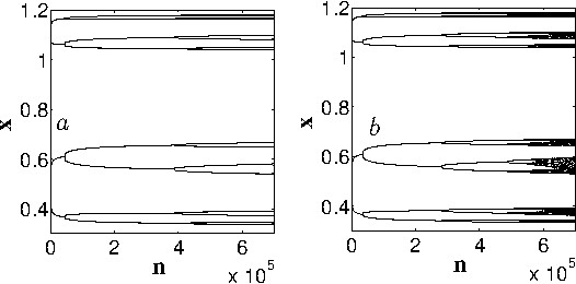
Figure 1: Two examples of cascade of bifurcations type trajectories in the Caputo logistic $\alpha$-family of maps (Eq.(15) with $T=1$ and $G_{K}(x)=x-Kx(1-x)$ ) with $\alpha=0.1$ and $x_{0}=0.001$: (a) for the nonlinearity parameter $K=22.39$ the last bifurcation from period $T=16$ to period $T=32$ occurs after approximately $7\times 10^{5}$ iterations; (b) when $K=22.416$ the trajectory becomes chaotic after approximately $6\times 10^{5}$ iterations.

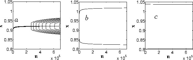
Figure 2: Asymptotically period two trajectories for the Caputo logistic $\alpha$-family of maps with $\alpha=0.1$ and $K=15.5$: (a) nine trajectories with initial conditions $x_{0}$ from 0.29 (the rightmost bifurcation) to 0.37 (the leftmost bifurcation) with the step 0.01; (b) $x_{0}=0.74$; (c) $x_{0}=0.94$.

3.1 $T=2$ sinks and stability of fixed points

Stability of fixed points in fractional dynamical systems was investigated in multiple publications, see, e.g., articles StA ; StL ; StM , chapter 4 in book Petras , and review StRev2013 ; for stability in discrete fractional systems see, e.g., StB ; ME1 ; StDis1 . There are various ways to define stability and various methods and criteria to analyze it. In this paper we consider an asymptotic stability of periodic points. A periodic point is asymptotically stable if there exists an open set such that all trajectories with initial conditions from this set converge to this point as $t\rightarrow\infty$. It is known from the study of the ordinary nonlinear dynamical systems that as a nonliniearity parameter increases the system bifurcates. This means that at the point (value of the parameter) of birth of the $T=2^{n+1}$ sink, the $T=2^{n}$ sink becomes unstable. In this section we will investigate the $T=2$ sinks of discrete fractional systems and apply our results to analyze stability of the systems’ fixed points. As all published results on the existence and stability of the $T=2$ point were obtained for $h=1$, in this section we assume $h=1$.

All published results on the asymptotic stability of the stable fixed point and $T=2$ sink were obtained for the fractional and fractional difference standard and logistic $\alpha$-families of maps.

Fractional standard map ($1<\alpha<2$)

First results on the first bifurcation and stability of the fixed point in discrete fractional systems were obtained in ME2 ; ME1 ; ME5 for the Riemann-Liouville standard $\alpha$-family of maps ($G_{K}(x)=K\sin(x)$) for $1<\alpha<2$. In this case the map Eq. (14) can be written as a two-dimensional map considered on a cylinder

$$p_{n+1}=p_{n}-K\sin x_{n},$$ (38)

$$x_{n+1}=\frac{1}{\Gamma(\alpha)}\sum_{i=0}^{n}p_{i+1}V^{1}_{\alpha}(n-i+1),\ \ \ \ ({\rm mod}\ 2\pi),$$ (39)

where

$$V^{k}_{\alpha}(m)=m^{\alpha-k}-(m-1)^{\alpha-k}$$ (40)

and the momentum $p(t)$ is defined as

$$p(t)=\,_{0}D^{\alpha-1}_{t}x(t).$$ (41)

The Caputo standard $\alpha$-family of maps from Eq. (15) can be considered on a torus and written as

$$p_{n+1}=p_{n}-\frac{K}{\Gamma(\alpha-1)}\Bigl{[}\sum_{i=0}^{n-1}V^{2}_{\alpha}(n-i+1)\sin x_{i}+\sin x_{n}\Bigr{]},\ \ ({\rm mod}\ 2\pi),$$ (42)

$$x_{n+1}=x_{n}+p_{0}-\frac{K}{\Gamma(\alpha)}\sum_{i=0}^{n}V^{1}_{\alpha}(n-i+1)\sin x_{i},\ \ ({\rm mod}\ 2\pi).$$ (43)

Both maps have the fixed point in the origin $(0,0)$. Numerical simulations show that both maps also have two $T=2$ sinks: the antisymmetric sink, with

$$p_{n+1}=-p_{n},\ \ x_{n+1}=-x_{n},$$ (44)

and the $\pi$-shift sink, with

$$p_{n+1}=-p_{n},\ \ x_{n+1}=x_{n}-\pi.$$ (45)

For the Riemann-Liouville family of maps there are two types of convergence of the trajectories to the fixed point and the $T=2$ sinks: fast (from the basins of attraction) with

$$\delta x_{n}\sim n^{-1-\alpha},\ \ \delta p_{n}\sim n^{-\alpha}$$ (46)

and slow with

$$\delta x_{n}\sim n^{-\alpha},\ \ \delta p_{n}\sim n^{1-\alpha}.$$ (47)

For the Caputo family of maps

$$\delta x_{n}\sim n^{1-\alpha},\ \ \delta p_{n}\sim n^{1-\alpha}.$$ (48)

The antisymmetric $T=2$ sink $(x_{l},p_{l})$ and $(-x_{l},-p_{l})$, Eq. (44), can be found considering the $n\rightarrow\infty$ limit in Eqs. (38) and (39):

$$p_{l}=\frac{K}{2}\sin(x_{l}),$$ (49)

$$x_{l}=\frac{K}{2\Gamma(\alpha)}V_{\alpha l}\sin(x_{l}),$$ (50)

where

$$V_{\alpha l}=\sum_{k=1}^{\infty}(-1)^{k+1}V_{\alpha}^{1}(k).$$ (51)

A high accuracy algorithm for calculating the slow converging series in Eq. (51) can be found in the Appendix section of ME4 . Eq. (50) has a solution and the $T=2$ sink exists when

$$K\geq K_{s1}(\alpha)=\frac{2\Gamma(\alpha)}{V_{\alpha l}}.$$ (52)

The opposite condition, as found in ME1 , is the condition of the stability of the $(0,0)$ fixed point. The same condition can be shown for the Caputo standard $\alpha$-family of maps. It is used to plot the part $1<\alpha\leq 2$ of the bottom thin line in Fig. 5 $a$, which is a two-dimensional ($\alpha-K$) bifurcation diagram. The fixed point (0,0) is stable below this line.

$\pi$-shift $T=2$ sink

$$p_{n}=(-1)^{n}p_{l},\ \ x_{n}=x_{l}-\frac{\pi}{2}[1-(-1)^{n}]$$ (53)

can be found plugging the asymptotic expression for $x_{n}$ from Eq. (53) and

$$p_{n}=(-1)^{n}p_{l}+An^{1-\alpha}$$ (54)

into Eqs. (38) and (39) and considering $n\rightarrow\infty$ limit. This gives

$$p_{l}=K/2\sin(x_{l}),\ \ A=\frac{2x_{l}-\pi}{2\Gamma(2-\alpha)},$$ (55)

$$\sin(x_{l})=\frac{\pi\Gamma(\alpha)}{KV_{\alpha l}},$$ (56)

which has solutions for

$$K>K_{s2}=\frac{\pi\Gamma(\alpha)}{V_{\alpha l}}=\frac{\pi}{2}K_{s1}.$$ (57)

$K_{s2}(\alpha)$ is used to plot the part $1<\alpha\leq 2$ of the middle thin line in Fig. 5 $a$.

Fractional logistic map ($1<\alpha\leq 2$)

A fractional generalization of the logistic map became possible after a small time delay was introduced into the differential equation describing a periodically kicked system Eq. (12) (see ME4 ). The logistic Riemann-Liouville $\alpha$-family of maps ($G_{K}(x)=x-Kx(1-x)$) can be written as

$$p_{n+1}=p_{n}+Kx_{n}(1-x_{n})-x_{n},$$ (58)

$$x_{n+1}=\frac{1}{\Gamma(\alpha)}\sum_{i=0}^{n}p_{i+1}V^{1}_{\alpha}(n-i+1).$$ (59)

Numerical simulations show that for $0<K\leq 1$ all converging trajectories converge to the fixed point $(0,0)$ as $x\sim n^{-\alpha-1}$, $p\sim n^{-\alpha}$. For $1<K<K_{l1}$ the only stable periodic sink is the fixed point $((K-1)/K,0)$. The rate of convergence to this fixed point is $\delta x\sim n^{-\alpha}$, $p\sim n^{-\alpha+1}$. At $K=K_{l1}$ the fixed point becomes unstable and the stable antisymmetric in $p$ period two sink appears. From the results of numerical simulations ME4 , the asymptotic behavior of converging to the $T=2$ sink trajectories follows the power law

$$p_{n}=p_{l}(-1)^{n}+\frac{A}{n^{\alpha-1}}.\ \$$ (60)

Substituting this expression for $p_{n}$ into Eq. (59) and considering even values of $n$, we obtain

$$x_{lo}=\lim_{n\rightarrow\infty}x_{2n+1}=\frac{p_{l}}{\Gamma(\alpha)}\lim_{n\rightarrow\infty}\sum^{2n+1}_{k=1}(-1)^{k}V_{\alpha}^{1}(k)$$

$$+\frac{A}{\Gamma(\alpha)}\lim_{n\rightarrow\infty}\sum^{2n-1}_{k=1}\frac{\alpha-1}{k^{\alpha-1}(2n-k)^{2-\alpha}}=-\frac{p_{l}}{\Gamma(\alpha)}V_{\alpha l}$$ (61)

$$+\frac{(\alpha-1)A}{\Gamma(\alpha)}\int^{1}_{0}\frac{x^{1-\alpha}dx}{(1-x)^{2-\alpha}}=-\frac{p_{l}}{\Gamma(\alpha)}V_{\alpha l}+A\Gamma(2-\alpha).$$

Here we took into account that the sum on the second line of the last equation is the Riemann sum for the integral on the third line, which is equal to the Beta-function $B(2-\alpha,\alpha-1)=\Gamma(2-\alpha)\Gamma(\alpha-1)$. Similarly,

$$x_{le}=\lim_{n\rightarrow\infty}x_{2n}=\frac{p_{l}}{\Gamma(\alpha)}V_{\alpha l}+A\Gamma(2-\alpha).$$ (62)

Then, in the limit $n\rightarrow\infty$, Eq. (58) gives

$$-2p_{l}=Kx_{le}(1-x_{le})-x_{le},$$ (63)

$$2p_{l}=Kx_{lo}(1-x_{lo})-x_{lo}.$$ (64)

Two fixed points, $x_{lo}=x_{le}=p_{l}=A=0$ and $x_{lo}=x_{le}=x_{l}=(K-1)/K$, $p_{l}=0$, $A=x_{l}/\Gamma(2-\alpha)$, are the two expected solutions of the system of four equations Eqs. (61)-(64). For the two remaining solutions with $x_{lo}\neq x_{le}$

$$A=\frac{K-1+\frac{2\Gamma(\alpha)}{V_{\alpha l}}}{2K\Gamma(2-\alpha)}$$ (65)

and the quadratic equation defining $x_{le}$ and $x_{lo}$ can be written as

$$x_{lo,le}^{2}-\Bigl{(}\frac{2\Gamma(\alpha)}{V_{\alpha l}K}+\frac{K-1}{K}\Bigr{)}x_{lo,le}+\frac{2\Gamma^{2}(\alpha)}{(V_{\alpha l}K)^{2}}+\frac{(K-1)\Gamma(\alpha)}{V_{\alpha l}K^{2}}=0.$$ (66)

The solutions of this equation

$$x_{lo,le}=\frac{K_{s1}+K-1\pm\sqrt{(K-1)^{2}-K_{s1}^{2}}}{2K}$$ (67)

are defined when

$$K\geq 1+\frac{2\Gamma(\alpha)}{V_{\alpha l}}=1+K_{s1}\ \ {\rm or}\ \ K\leq 1-\frac{2\Gamma(\alpha)}{V_{\alpha l}}=1-K_{s1}.$$ (68)

From $V_{\alpha l}<1$ and $\Gamma(\alpha)>0.885$ for $\alpha>0$ follows that $2\Gamma(\alpha)/V_{\alpha l}>1$ and, considering only $K>0$, we may ignore the second of the inequalities in Eq. (68). We may also note that the fixed point $x=(K-1)/K$ is stable when

$$1\leq K<K_{l1}=1+\frac{2\Gamma(\alpha)}{V_{\alpha l}}=1+K_{s1}.$$ (69)

$K_{l1}(\alpha)$ is used to plot the part $1<\alpha\leq 2$ of the bottom thin line in Fig. 5 $b$.

Fractional and fractional difference standard $\alpha$-families of maps for $0<\alpha<1$

In this and the next sections we will follow the results obtained in ME8 . For $0<\alpha<1$ fractional and fractional difference maps, Eq. (15) and Eq. (35), can be written (with $h=1$ and $G_{K}(x)=K\sin(x)$) in the universal form

$$x_{n}=x_{0}-\frac{K}{\Gamma(\alpha)}\sum^{n-1}_{k=0}W_{\alpha}(n-k)\sin{(x_{k})},$$ (70)

where $W_{\alpha}(s)=s^{\alpha-1}$ for the fractional map and $W_{\alpha}(s)={\Gamma(s+\alpha-1)}/{\Gamma(s)}$ for the fractional difference map.

For $\alpha=0$ the Caputo fractional standard map is identically zero and fractional difference is the sine map

$$x_{n+1}=-K\sin(x_{n}),\ \ \ ({\rm mod}\ 2\pi).$$ (71)

For $\alpha=1$ both maps converge to the circle map with zero driven phase

$$x_{n+1}=x_{n}+K\sin(x_{n}),\ \ \ \ ({\rm mod}\ 2\pi).$$ (72)

In the sine map and in the circle map with zero driven phase, when the $x=0$ sink becomes unstable, it bifurcates into the symmetric $T=2$ sink in which $x_{n+1}=-x_{n}$. Following the results of ME8 , let’s assume that this property persists (asymptotically) for $\alpha\in(0,1)$. Eq. (70) can be written as

$$x_{n+1}=x_{n}-\frac{K}{\Gamma(\alpha)}\Bigl{\{}W_{\alpha}(1)\sin{(x_{n})}$$

$$+\sum^{n-1}_{k=0}\sin{(x_{k})}[W_{\alpha}(n-k+1)-W_{\alpha}(n-k)]\Bigr{\}}.$$ (73)

Because $W_{\alpha}(n-k+1)-W_{\alpha}(n-k)\rightarrow 0$ when $n\rightarrow\infty$, substituting $j=n-k$, asymptotically for large $n$ Eq. (73) can be written as

$$x_{n}=\frac{K}{2\Gamma(\alpha)}\Bigl{\{}W_{\alpha}(1)+\sum^{\infty}_{j=1}(-1)^{j}[W_{\alpha}(j+1)-W_{\alpha}(j)]\Bigr{\}}\sin{(x_{n})},$$ (74)

where the alternating series on the right side converges because its terms converge to 0 monotonically. This equation has real non-trivial solutions when

$$K>K_{s1}=\frac{2\Gamma(\alpha)}{W_{\alpha}(1)+\sum^{\infty}_{j=1}(-1)^{j}[W_{\alpha}(j+1)-W_{\alpha}(j)]}.$$ (75)

This expression for $K_{s1}$ is used to plot the parts $0<\alpha\leq 1$ of the bottom thin and bold lines in Fig. 5 $a$.

When the symmetric $T=2$ sink becomes unstable it gives birth to the $\pi$-shift $T=2$ sink in which $|x_{n+1}-x_{n}|=\pi$. The asymptotic analysis similar to the above performed for the symmetric $T=2$ sink yields the following equation to define the asymptotic values for this sink

$$\pm\pi=\frac{K}{\Gamma(\alpha)}\Bigl{\{}W_{\alpha}(1)+\sum^{\infty}_{j=1}(-1)^{j}[W_{\alpha}(j+1)-W_{\alpha}(j)]\Bigr{\}}\sin{(x_{n})},$$ (76)

which has solutions when

$$K>K_{s2}=\pi K_{s1}/2.$$ (77)

This expression for $K_{s2}$ is used to plot the part $0<\alpha\leq 1$ of the middle thin line in Fig. 5 $a$. It also could be used to calculate the middle bold line, but in this paper we use the results of the direct numerical calculations ME8 instead. The difference between the results of the direct numerical simulations and the calculations using Eq. (77) is evident when $\alpha<0.15$. This difference is due to the slow, as $n^{-\alpha}$, convergence of trajectories.

Fractional difference standard $\alpha$-families of maps for $1<\alpha<2$

When $1<\alpha<2$ the fractional difference Caputo standard $\alpha$-FM Eq. (35) can be written as a two-dimensional map ME8

$$p_{n}=p_{1}-\frac{K}{\Gamma(\alpha-1)}\times\sum^{n}_{s=2}\frac{\Gamma(n-s+\alpha-1)}{\Gamma(n-s+1)}\sin(x_{s-1}),\ \ ({\rm mod}\ 2\pi),$$ (78)

$$x_{n}=x_{n-1}+p_{n},\ \ ({\rm mod}\ 2\pi),\ \ n\geq 1,$$ (79)

where $p_{n}=\Delta x_{n-1}=x_{n}-x_{n-1}$.

As in the fractional standard map, in the fractional difference standard map, when the $(0,0)$ fixed point becomes unstable, it bifurcates into the $T=2$ antisymmetric sink $x_{n+1}=-x_{n}$, $p_{n+1}=-p_{n}$, which later, at $K$ for which $x_{n}=\pi/2$, turns into two $\pi$-shift $T=2$ sinks ME8 . For the anti-symmetric sink, in the limit $n\rightarrow\infty$ Eq. (79) yields $p_{n}=2x_{n}$ and Eq. (78)

$$p_{n}=\frac{K}{2\Gamma(\alpha-1)}\Bigl{\{}W_{\alpha-1}(1)+\sum^{\infty}_{j=1}(-1)^{j}[W_{\alpha-1}(j+1)-W_{\alpha-1}(j)]\Bigr{\}}\sin{(x_{n})},$$ (80)

where, as in Eq (70), $W_{\alpha}(s)={\Gamma(s+\alpha-1)}/{\Gamma(s)}$. The equations for the antisymmetric $T=2$ sink $(x_{n},p_{n})$ are

$$x_{n}=\frac{K}{4\Gamma(\alpha-1)}\Bigl{\{}W_{\alpha-1}(1)+\sum^{\infty}_{j=1}(-1)^{j}[W_{\alpha-1}(j+1)-W_{\alpha-1}(j)]\Bigr{\}}\sin{(x_{n})},$$ (81)

$$p_{n}=2x_{n}.$$ (82)

They have solutions for

$$K>K_{s1}(\alpha)=2K_{s1}(\alpha-1),$$ (83)

where $K_{c1d}(\alpha-1)$ is defined by Eq. (75). This result is used to plot the part $1<\alpha\leq 2$ of the bottom bold line in Fig. 5 $a$.

Equations defining the $\pi$-shift $T=2$ sink can be written as

$$\pm\pi=\frac{K}{2\Gamma(\alpha-1)}\Bigl{\{}W_{\alpha-1}(1)+\sum^{\infty}_{j=1}(-1)^{j}[W_{\alpha-1}(j+1)-W_{\alpha-1}(j)]\Bigr{\}}\sin{(x_{n})},$$ (84)

$$p_{n}=\pm\pi.$$ (85)

$\pi$-shift sink exists when

$$K>K_{s2}(\alpha)=\frac{\pi}{2}K_{s1}(\alpha).$$ (86)

This result is used to plot the part $1<\alpha\leq 2$ of the middle bold line in Fig. 5 $a$.

The fixed point in the origin is stable for $K<K_{s1}$ and the convergence of trajectories to the fixed point follows the power law $x_{n}\sim n^{1-\alpha}$ and $p_{n}\sim n^{-\alpha}$.

3.2 $T=2^{n}$ sinks

Investigation of the $T=2^{n}$-sinks’ stability with $n>2$ by analytic methods is complicated. In papers ME2 ; ME3 ; ME4 ; ME6 ; ME7 ; ME8 ; ME9 ; Chaos2015 ; ME1 ; ME5 this is done by numerical simulations on individual trajectories with various values of parameters ($K$ and $\alpha$) and initial conditions. As in the case of the fixed point and $T=2$-sink, stability of the high order sinks is asymptotic. Trajectories, which converge to $T=2^{n}$-sinks ($n^{th}$ order sinks) stable in the limit $n\rightarrow\infty$, may first converge to low order sinks and then, through cascades of period doubling bifurcations, converge to the sinks of the $n^{th}$ order. Cascade of bifurcations type trajectories are the fundamental features of the discrete fractional systems. Their presence makes drawing of various kinds of fractional bifurcation diagrams (the subject of the next section) difficult. Fractional bifurcation diagrams strongly depend on the number of iterations and initial conditions of individual trajectories used in the analysis. The larger the number of iterations used in the calculations, the closer the calculated values of the sinks to their limiting values.

4 Fractional bifurcation diagrams

Fractional maps demonstrate the universal scenario of transition to chaos through the period doubling cascade of bifurcations with the change in a nonlinearity parameter, similar to the one described in May . This is illustrated in Fig. 3, in which the bifurcation diagrams ($x$ vs. $K$) for various considered families of maps with $\alpha=0.8$ are presented. Compared to the integer case $\alpha=1$, bifurcation diagrams for the fractional maps are stretched along the $K$ axis while bifurcation diagrams for the fractional difference maps are contracted. The existence of self-similarity, corresponding constants (analogs of the Feigenbaum constants), and their dependence on $\alpha$ in fractional maps are not investigated.

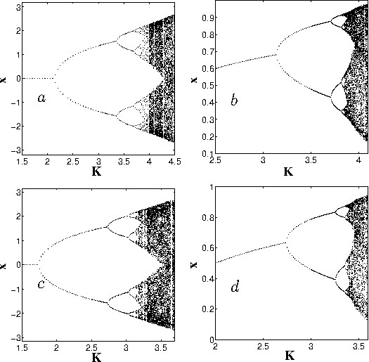
Figure 3: The bifurcation diagrams for fractional Caputo standard (a) and logistic (b) maps and for fractional difference Caputo standard (c) and logistic (d) maps with $\alpha=0.8$.

The dependence of the bifurcation diagrams on the number of iterations is demonstrated in Fig. 4. Bifurcation diagrams obtained after five thousand iteration look much nicer than those obtained after two hundred. But, as it follows from Figs. 1 and 2, even 5000 iterations are not enough for computation of the asymptotic bifurcation diagrams.

The two-dimensional bifurcation diagrams Fig. 5 are obtained by combining the results of the computations of the bifurcation ($x$ vs. $K$) diagrams after 5000 iterations for fixed values of $\alpha$. Because for small $\alpha$ convergence of trajectories to their asymptotic values is very slow, the results in the diagrams for $\alpha<0.15$ do not represent well the asymptotic values and can be improved in future.

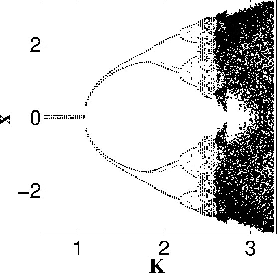
Figure 4: Two bifurcation diagrams for the fractional difference Caputo Standard $\alpha$FM with $\alpha=0.1$ and $x_{0}=0.1$ calculated after 200 iterations (regular points) and 5000 iterations (bold points). This figure is reprinted from ME8 , with the permission of AIP Publishing.

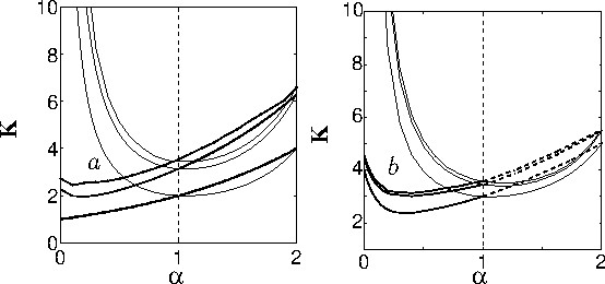
Figure 5: 2D bifurcation diagrams for fractional (thing lines) and fractional difference (bold lines) Caputo standard (a) and logistic (b) maps. First bifurcation, transition from the stable fixed point to the stable period two ($T=2$) sink, occurs on the bottom curves. $T=2$ sink (in the case of the standard $\alpha$-families of maps, antisymmetric T=2 sink with $x_{n+1}=-x_{n}$) is stable between the bottom and the middle curves. Transition to chaos occurs on the top curves. Period doubling bifurcations leading to chaos occur in the narrow band between the middle and the top curves. The bottom curves in (a) are obtained using Eqs. (52), (75), and (83). The thin middle curve in (a) is obtained using Eqs. (57) and (77). The $1<\alpha\leq 2$ part of the middle bold line in (a) is obtained using Eq. (86). The $1<\alpha\leq 2$ part of the bottom thin line in (b) is obtained using Eq. (69). The remaining curves, except the bold dashed curves in (b), are results of the direct numerical simulations. The bold dashed curves in (b) are obtained by interpolation.

Looking at the 2D bifurcation diagrams one may note that systems with power-law memory should demonstrate bifurcations with changes in the memory parameter $\alpha$ when the nonlinearity parameter $K$ stays constant. This property of systems with power-law memory is demonstrated in Fig. 6 and it may explain how changes/failures in live biological species can be caused by changes in their memory and nervous system. This also may explain how some diseases may be treated by treating the nervous system.

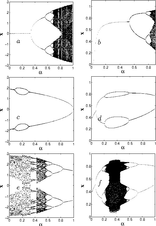
Figure 6: The memory $\alpha$-bifurcation diagrams for fractional Caputo standard (a) and logistic (b) maps and for fractional difference Caputo standard (c) and (e) and logistic (d) and (f) maps obtained after 5000 iteration. $K=4.2$ in (a), $K=3.8$ in (b), $K=2.0$ in (c), $K=3.1$ in (d), $K=2.8$ in (e), and $K=3.2$ in (7).

5 Conclusion

The following citation from Wikipedia, “universality is the observation that there are properties for a large class of systems that are independent of the dynamical details of the system”, defines the notion of the universality in dynamical systems. The universality in systems with power-law memory goes beyond the period doubling with changes in nonlinearity and memory parameters and the universal scenario of transition to chaos. Individual trajectories of such systems also demonstrate cascade of bifurcations type behavior. In regular dynamics the universality has a mathematical expression in the form of the Feigenbaum function and constants. This is only the beginning of the research on fractional universality and most of the results are obtained by numerical simulations. Those results introduce more questions than answers. Some of those questions are:

• What is the nature and the corresponding analytic description of the bifurcations on a single trajectory of a fractional system?

• What kind of self-similarity can be found in CBTT?

• How to describe a self-similar behavior corresponding to the bifurcation diagrams of fractional systems? Can constants, similar to the Feigenbaum constants be found?

• Can cascade of bifurcations type trajectories be found in continuous systems?

Behavior of fractional systems at low values of $\alpha$ ($0<\alpha<0.15$) is very important in biological applications but is not well established and requires an additional investigation.

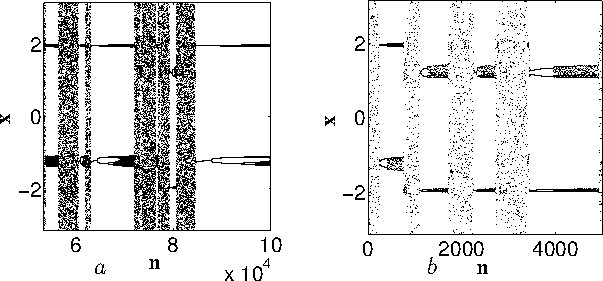
Figure 7: Intermittent cascade of bifurcations type trajectories for the Caputo ($a$) and fractional difference Caputo ($b$) Standard $\alpha$FMs. In ($a$) $\alpha=1.65$, $K=4.5$, $x_{0}=0.$, and $p_{0}=0.3$. In ($b$) $\alpha=1.5$, $K=4.82$, $x_{0}=0.$, and $p_{0}=0.01$. This figure is reprinted from ME9 , with the permission of L&H Scientific Publishing.

As mentioned in the introduction, there is a possibility for multiple applications of the fractional universality in biology. The human body is a system with power-law memory, which implies the possibility of medical applications. Fig. 2 $a$ suggests that, assuming some distribution (e.g., uniform) of the initial conditions of an asymptotically $T=2$ system with power-law memory, it is possible to calculate the probability distribution of times before the stable fixed point behavior of the system bifurcates. Comparison of probability distributions for various values of $K$ and $\alpha$ to the statistics of the times before sudden changes (e.g., deaths) after serious surgeries (e.g., heart transplants) may help to understand the state of a human body after the surgery and suggest some remedies.

The intermittent cascade of bifurcations type behavior is typical for systems with power-law memory (see Fig. 7). May this intermittency explain the intermittent behavior, transitions from stability to chaos and back to stability, in various socio-economic systems, which are systems with power-law memory? May the history of human society, with repeating periods of dictatorship, democracy, and chaos, be modeled by the equations with power-law memory? There are many questions related to the topic of this review which motivate research on systems with power-law memory.

- (1) Aguila-Camacho, N. and Duarte-Mermoud, M.A., and Gallegos, J.A.: Lyapunov functions for fractional order systems. Commun. Nonlin. Sci. Numer. Simul. 19, 2951 -2957 (2014)
- (2) Anderson, J.R.: Learning and memory: An integrated approach. Wiley, New York 1(995)
- (3) Anastassiou, G.A.: Nabla discrete fractional calculus and nabla inequalities. Math. Comput. Modelling 51, 562–571 (2010)
- (4) Atici, F. and Eloe P.: Initial value problems in discrete fractional calculus. Proc. Am. Math. Soc. 137, 981–989 (2009)
- (5) Atici, F. and Eloe P.: Discrete fractional calculus with the nabla operator. Electron. J. Qual. Theory Differ. Equ. Spec. Ed. I3, 1–12 (2009)
- (6) Baleanu, D., Wu, G.-C., Bai, Y.-R., and Chen, F.-L.: Stability analysis of Caputo-like discrete fractional systems. Commun. Nonlin. Sci. Numer. Simul. 48, 520–530 (2017)
- (7) Bastos, N.R.O., Ferreira, R.A.C., and Torres D.F.M.: Discrete-time fractional variational problems. Signal Processing 91, 513–524 (2011)
- (8) Bastos, N.R.O., Ferreira, R.A.C., and Torres D.F.M.: Necessary optimality conditions for fractional difference problems of the calculus of variations. Discrete Contin. Dyn. Syst. 29, 417–437 (2011)
- (9) Chen, F., Luo, X., and Zhou, Y.: Existence Results for Nonlinear Fractional Difference Equation. Adv.Differ.Eq. 2011, 713201, (2011)
- (10) Cvitanovic, P.: Universality in Chaos. Adam Hilger, Bristol and New York (1989)
- (11) Edelman,M.: Fractional Standard Map: Riemann-Liouville vs. Caputo. Commun. Nonlin. Sci. Numer. Simul. 16, 4573–4580 (2011)
- (12) Edelman, M.: Fractional Maps and Fractional Attractors. Part I: -Families of Maps. Discontinuity, Nonlinearity, and Complexity 1, 305–324 (2013)
- (13) Edelman, M.: Universal Fractional Map and Cascade of Bifurcations Type Attractors. Chaos 23, 033127 (2013)
- (14) Edelman, M.: Universality in fractional dynamics. International Conference on Fractional Differentiation and Its Applications (ICFDA), 2014, DOI: 10.1109/ICFDA.2014.6967376, (2014), Page(s): 1–6
- (15) Edelman, M.: Fractional Maps as Maps with Power-Law Memory. In: Eds.: Afraimovich, A., Luo, A.C.J., Fu, X. (eds.): Nonlinear Dynamics and Complexity; Series: Nonlinear Systems and Complexity, 79–120, New York, Springer (2014)
- (16) Edelman, M.: Caputo standard -family of maps: Fractional difference vs. fractional. Chaos 24, 023137 (2014)
- (17) Edelman, M.: Fractional Maps and Fractional Attractors. Part II: Fractional Difference -Families of Maps. Discontinuity, Nonlinearity, and Complexity 4, 391–402 (2015)
- (18) Edelman, M.: On the fractional Eulerian numbers and equivalence of maps with long term power-law memory (integral Volterra equations of the second kind) to Grnvald-Letnikov fractional difference (differential) equations. Chaos 25, 073103 (2015).
- (19) Edelman, M., Tarasov, V.E.: Fractional standard map. Phys. Lett. A 374, 279–285 (2009)
- (20) Edelman, M., Taieb, L.A.: New types of solutions of non-linear fractional differential equations. In: Almeida, A., Castro, L., Speck F.-O. (eds.) Advances in Harmonic Analysis and Operator Theory; Series: Operator Theory: Advances and Applications. 229, 139–155 Springer, Basel (2013)
- (21) Fairhall, A.L., Lewen, G.D., Bialek, W., de Ruyter van Steveninck R.R.: Efficiency and Ambiguity in an Adaptive Neural Code. Nature 787–792 (2001)
- (22) Ferreira, R.A.C. and Torres D.F.M.: Fractional h-difference equations arising from the calculus of variations. Appl. Anal. Discrete Math. 5, 110–121 (2011)
- (23) Frederico, G.S.F. and Torres D.F.M.: A formulation of Noether’s theorem for fractional problems of the calculus of variations. J. Math. Appl. Anal. Appl. 334, 834–846 (2007)
- (24) Gray, H.L. and Zhang, N.-F.: On a new definition of the fractional difference. Math. Comput. 50, 513–529 (1988)
- (25) Kahana, M.J.: Foundations of human memory. Oxford University Press, New York (2012)
- (26) Kilbas, A.A., Bonilla, B., and Trujillo, J.J.: Nonlinear differential equations of fractional order is space of integrable functions. Dokl. Math. 62, 222–226 (2000)
- (27) Kilbas, A.A., Bonilla, B., and Trujillo, J.J.: Existence and uniqueness theorems for nonlinear fractional differential equations. Demonstratio Math. 33, 583–602 (2000)
- (28) Kilbas, A.A., Srivastava, H.M., and Trujillo, J.J.: Theory and Application of Fractional Differential Equations. Elsevier, Amsterdam (2006)
- (29) Leopold D.A., Murayama, Y,, Logothetis, N.K.: Very slow activity fluctuations in monkey visual cortex: implications for functional brain imaging. Cerebr Cortex 413, 422–433 (2003)
- (30) Li, Y., Chen, Y.Q., and Podlubny, I.: Stability of fractional-order nonlinear dynamic systems: Lyapunov direct method and generalized Mittag-Leffler stability. Comput. Math. Appl. 59, 1810 -21 (2010)
- (31) Lundstrom, B.N., Fairhall, A.L., Maravall, M.: Multiple time scale encoding of slowly varying whisker stimulus envelope incortical and thalamic neurons in vivo. J. Neurosci 30, 5071–5077 (2010)
- (32) Lundstrom, B.N., Higgs, M.H., Spain, W.J., Fairhall, A.L.: Fractional differentiation by neocortical pyramidal neurons. Nat Neurosci 11, 1335–1342 (2008)
- (33) Machado,J.A. Tenreiro, Pinto, Carla M.A., Lopes, A. Mendes: A review on the characterization of signals and systems by power law distributions. Signal Process 107, 246–253 (2015)
- (34) Matignon, D.: Stability properties for generalized fractional differential systems. ESAIM Proc. 5, 145–58 (1998)
- (35) May, R.M.: Simple mathematical models with very complicated dynamics. Nature 261, 459–467 (1976)
- (36) Miller, K.S. and Ross, B.: Fractional Difference Calculus. In: Srivastava, H.M. and Owa, S. (eds.) Univalent Functions, Fractional Calculus, and Their Applications. 139–151 Ellis Howard, Chichester, (1989)
- (37) Mozyrska, D. and Girejko, E.: Overview of the fractional h-difference operators. In: Almeida, A., Castro, L., Speck F.-O. (eds.) Advances in Harmonic Analysis and Operator Theory; Series: Operator Theory: Advances and Applications. 229, 253–267 Springer, Basel (2013)
- (38) Mozyrska, D. and Girejko, E., and Wirwas, M.: Fractional nonlinear systems with sequential operators. Cent. Eur. J. Phys. 11, 1295–1303 (2013)
- (39) Mozyrska, D. and Pawluszewicz E.: Local controllability of nonlinear discrete-time fractional order systems. Bull. Pol. Acad. Sci. Techn. Sci. 61, 251–256 (2013)
- (40) Mozyrska, D., Pawluszewicz E., and Girejko, E.: Stability of nonlinear h-difference systems with N fractional orders. Kibernetica 51, 112–136 (2015)
- (41) Petras, I.: Fractional-Order Nonlinear Systems. Springer, Berlin, (2011)
- (42) Podlubny, I.: Fractional Differential Equations. Academic Press, San Diego (1999)
- (43) Pozzorini, C., Naud, R., Mensi, S., Gerstner, W.: Temporal whitening by power-law adaptation in neocortical neurons. Nat Neurosci 16, 942–948 (2013)
- (44) Rivero, M., Rogozin, S.V., Machado, J.A.T., and Trujilo, J.J.: Stability of fractional order systems. Math. Probl. Eng. 2013, 356215 (2013)
- (45) Rubin, D.C., Wenzel, A.E.: One Hundred Years of Forgetting: A Quantitative Description of Retention. Psychol Rev 103, 743–760 (1996)
- (46) Samko, S.G., Kilbas, A.A., and Marichev, O.I.: Fractional Integrals and Derivatives Theory and Applications. Gordon and Breach, New York (1993)
- (47) Stanislavsky, A.A: Long-term memory contribution as applied to the motion of discrete dynamical system. Chaos 16, 043105 (2006)
- (48) Tarasov, V.E.: Differential equations with fractional derivative and universal map with memory. J. Phys. A 42, 465102 (2009)
- (49) Tarasov, V.E.: Discrete map with memory from fractional differential equation of arbitrary positive order J. Math. Phys. 50, 122703 (2009)
- (50) Tarasov, V.E.: Fractional Dynamics: Application of Fractional Calculus to Dynamics of Particles, Fields and Media. HEP, Springer, Beijing, Berlin, Heidelberg (2011)
- (51) Tarasov, V.E., Zaslavsky, G.M.: Fractional equations of kicked systems and discrete maps. J. Phys. A 41, 435101 (2008)
- (52) Toib, A., Lyakhov, V., Marom, S.: Interaction between duration of activity and recovery from slow inactivation in mammalian brain Na+ channels. J Neurosci 18, 1893–1903 (1998)
- (53) Ulanovsky, N., Las, L., Farkas, D., Nelken, I.: Multiple time scales of adaptation in auditory cortex neurons. J Neurosci 24, 10440–10453 (2004)
- (54) Wixted, J.T.: Analyzing the empirical course of forgetting. J Exp Psychol Learn Mem Cognit 16, 927–935 (1990)
- (55) Wixted, J.T., Ebbesen, E.: On the form of forgetting. Psychol Sci 2, 409–415 (1991).
- (56) Wixted, J.T., Ebbesen, E.: Genuine power curves in forgetting. Mem Cognit 25, 731–739 (1997)
- (57) Wu, G.-C., Baleanu, D.: Discrete fractional logistic map and its chaos. Nonlin. Dyn. 75, 283–287 (2014)
- (58) Wu, G.-C., Baleanu, D., Zeng, S.-D.: Discrete chaos in fractional sine and standard maps. Phys. Lett. A 378, 484–487 (2014)
- (59) Wyrwas, M., Pawluszewicz, E., and Girejko, E.: Stability of nonlinear -difference systems with fractional orders. Kybernetika 15, 112–136 (2015)
- (60) Zaslavsky, G.M.: Hamiltonian Chaos and Fractional Dynamics. Oxford University Press, Oxford (2005)
- (61) Zaslavsky, G.M., Stanislavsky, A.A., and Edelman, M: Chaotic and pseudochaotic attractors of perturbed fractional oscillator. Chaos 16, 013102 (2006)
- (62) Zilany, M.S., Bruce, I.C., Nelson, P.C., Carney, L.H.: A phenomenological model of the synapse between the inner hair cell and auditory nerve: long-term adaptation with power-law dynamics. J. Acoust. Soc. Am. 126, 2390–2412 (2009)