Two-Sample Instrumental Variable Analyses using Heterogeneous Samples

Abstract

Instrumental variable analysis is a widely used method to estimate causal effects in the presence of unmeasured confounding. When the instruments, exposure and outcome are not measured in the same sample, Angrist and Krueger (1992) suggested to use two-sample instrumental variable (TSIV) estimators that use sample moments from an instrument-exposure sample and an instrument-outcome sample. However, this method is biased if the two samples are from heterogeneous populations so that the distributions of the instruments are different. In linear structural equation models, we derive a new class of TSIV estimators that are robust to heterogeneous samples under the key assumption that the structural relations in the two samples are the same. The widely used two-sample two-stage least squares estimator belongs to this class. It is generally not asymptotically efficient, although we find that it performs similarly to the optimal TSIV estimator in most practical situations. We then attempt to relax the linearity assumption. We find that, unlike one-sample analyses, the TSIV estimator is not robust to misspecified exposure model. Additionally, to nonparametrically identify the magnitude of the causal effect, the noise in the exposure must have the same distributions in the two samples. However, this assumption is in general untestable because the exposure is not observed in one sample. Nonetheless, we may still identify the sign of the causal effect in the absence of homogeneity of the noise.

, , , and

1 Introduction

When randomized controlled experiments are not feasible, instrumental variable (IV) analysis is a widely used method to estimate causal effect in the presence of unmeasured confounding. A typical instrumental variable estimator such as the two-stage least squares (TSLS) uses sample moments (e.g. covariance matrices) of the instrument-exposure relationship and the instrument-outcome relationship. In an influential article, Angrist and Krueger (1992) noticed that the two sets of moments can indeed be estimated from different samples, though this idea can be dated back to at least Klevmarken (1982). This method, often referred to as the two-sample instrumental variable (TSIV) estimator, is frequently used in econometrics (Inoue and Solon, 2010).

One of the most exciting recent applications of IV analysis is in genetic epidemiology where genetic variants are used as the instruments (Davey Smith and Ebrahim, 2003, Lawlor et al., 2008, Burgess et al., 2015). This method is known as “Mendelian randomization” to epidemiologists, because the genotypes are governed by Mendel’s Second Law of independent assortment and thus have a strong rationale for being independent of common postnatal source of confounding. More recently, there has been growing interest in using two-sample Mendelian randomization that take advantage of large existing Genome-Wide Association Studies (GWAS), as it is often easier to find two GWAS in which one measures the genotypes and the exposure and the other one measures the genotypes and the disease than to find a single GWAS that measures all three types of variables (Pierce and Burgess, 2013, Davey Smith and Hemani, 2014, Burgess et al., 2015, Gamazon et al., 2015, Lawlor, 2016).

Since Mendelian randomization is a special case of instrumental variable analysis in which genetic variants are used as instruments, one would expect that two-sample Mendelian randomization is merely a different application of the existing TSIV estimators. However, there is a subtle but important difference between two-sample Mendelian randomization and the existing applications of TSIV in economic applications. To the best of our knowledge, with the exception of Graham et al. (2016) who considered a general data combination problem including just-identified TSIV, all the TSIV estimators previously proposed in econometrics assumed that the two datasets are sampled from the same population (Angrist and Krueger, 1992, Ridder and Moffitt, 2007, Inoue and Solon, 2010, Pacini and Windmeijer, 2016). This is usually not a problem in the economic applications using time-invariant instrumental variables (Jappelli et al., 1998) such as quarter of birth (Angrist and Krueger, 1992) and sex composition of the children in the household (Currie and Yelowitz, 2000). However, this assumption does not hold in two-sample Mendelian randomization, as the two GWAS usually consist of different cohort studies and thus represent different populations. Table 1 shows an example of two-sample Mendelian randomization in which the distribution of the genetic instruments are clearly different in the different populations.

Table 1: Heterogeneous distribution of genetic instruments in different populations. The minor allele frequencies in Table 1(a) and link disequilibrium $r^{2}$ in Table 1(b) are obtained from the 1000 Genome Project available in online databases dbSNP (Sherry et al., 2001) and LDlink (Machiela and Chanock, 2015). The SNPs are selected from the real data analysis in Section 8.

(a) Minor allele frequencies in different populations.

		Minor allele frequency
		African	East Asian	European	South Asian	American
		($n=1322$)	($n=1008$)	($n=1006$)	($n=978$)	($n=694$)
	rs13021737	0.095	0.087	0.174	0.13	0.14
SNP	rs1421085	0.056	0.169	0.432	0.31	0.24
	rs6567160	0.220	0.183	0.240	0.32	0.13

(b) Linkage disequilibrium (measured by $r^{2}$, the square of the correlation coefficient of allele indicators) in different populations.

		Linkage disequilibrium ($r^{2}$)
		African	East Asian	European	South Asian	American
		($n=1322$)	($n=1008$)	($n=1006$)	($n=978$)	($n=694$)
	(rs13021737, rs6731348)	0.378	1.0	0.993	0.865	0.965
SNP pair	(rs13021737, rs4854344)	0.917	1.0	0.993	0.865	0.988
	(rs6731348, rs4854344)	0.387	1.0	0.986	1.0	0.953

The goal of this paper is to clarify the consequences of heterogeneous samples to the identification, estimation, and robustness of TSIV analyses. After setting up the TSIV problem and reviewing the literature (Section 2), we will derive a new class of TSIV estimators using the generalized method of moments (GMM) that can utilize two heterogeneous samples under a linear IV model (Section 3). The commonly-used two-sample two-stage least squares (TSTSLS) belongs to this class of estimators, but unlike the case with homogeneous samples, it is no longer the most efficient estimator in this class. Another interesting question raised by epidemiologists and geneticists is how far we can get by using just public summary statistics of GWAS (Lawlor, 2016, Barbeira et al., 2016). Our calculations show that, to use correlated genetic IVs without individual-level data, it is necessary to use their covariance matrices (in both samples) to compute any TSIV estimator and its asymptotic variance. Unfortunately, the covariance information is often unavailable in the current GWAS summary databases, though it is possible to approximate the covariance matrices using external datasets such as the 1000 Genomes Project Consortium (2015).

We will then turn to relax the linearity assumption in Sections 4, 5 and 6. Compared to the same problem in the one-sample or the homogeneous two-sample setting, a key distinction is that we also need the structural relationships between the IV and the exposure and the distributions of the noise variables to be invariant in the two samples. Unfortunately, these assumptions are untestable using empirical data because we do not observe the exposure in both samples. In the absence of these assumptions, we show that one may still identify the sign of the causal effect.

Next we will use simulations to study the numerical properties of the TSIV estimators (Section 7). We find that although the asymptotic efficiency of TSTSLS is suboptimal theoretically, the difference in practice is most of the time minuscule. We will also examine the bias of the TSIV estimators when the instrument-exposure equation is misspecified or the “homogeneous noise” assumption is violated. We will also compare the results of the TSIV analyses with the classical one-sample analyses using a real Mendelian randomization dataset (Section 8). Finally, we will summarize the theoretical and empirical findings in Section 9. Although we will be using Mendelian randomization as the motivating application in the investigation below, we expect the statistical methods, identification results and high-level conclusions in this paper can be applied to TSIV analyses in other fields as well.

2 Background on TSIV analyses

In this section we set up the TSIV problem and review the related literature. For simplicity of exposition, throughout the paper we consider only one endogenous exposure variable and no other exogenous covariates for adjustment. Most of our derivations can be easily generalized to the case of multiple endogenous variables and multiple exogenous covariates.

2.1 Problem setup

We begin by introducing some notational conventions. We use lower-case letters, bold lower-case letters, bold upper-case letters, and Greek letters to indicate, respectively, deterministic or random scalars, vectors, matrices, and parameters in the model. Superscripts $s$, $a$, $b$ are reserved to indicate the sample. Subscripts are used to index the observations in each sample.

Suppose we have independent samples $(\mathbf{z}_{i}^{s},x_{i}^{s},y_{i}^{s}),~{}i=1,2,\dotsc,n^{s}$, from two populations, $s=a$ and $s=b$, where $\mathbf{z}\in\mathbb{R}^{q}$ is a vector of instrumental variables, $x$ is the exposure variable, and $y$ is the outcome variable. More compactly, we can write the data in each sample as a matrix $\mathbf{Z}^{s}\in\mathbb{R}^{n^{s}\times q}$ and two vectors $\mathbf{x}^{s},\mathbf{y}^{s}\in\mathbb{R}^{n^{s}}$. Next we describe the general setting in this paper.

Assumption 1.

The data are generated from the following nonparametric structural equation model (SEM). For $s\in\{a,b\}$,

$$y_{i}^{s} =g^{s}(x_{i}^{s},\mathbf{z}_{i}^{s},u_{i}^{s}),$$ (1)

$$x_{i}^{s} =f^{s}(\mathbf{z}_{i}^{s},v_{i}^{s}),$$ (2)

where the functions $g^{s}$, $f^{s}$ are unknown and the random variables $(u^{s}_{i},v^{s}_{i},\mathbf{z}^{s}_{i}),~{}i=1,\dotsc,n^{s}$ are independent and identically distributed within each sample.

Hereafter, (1) will be called the exposure-outcome equation or simply the outcome equation, and (2) the instrument-exposure equation or the exposure equation. The exposure variable $x$ is called endogenous if $v\not\mathchoice{\mathrel{\hbox to0.0pt{$\displaystyle\perp$\hss}\mkern 2.0mu{\displaystyle\perp}}}{\mathrel{\hbox to0.0pt{$\textstyle\perp$\hss}\mkern 2.0mu{\textstyle\perp}}}{\mathrel{\hbox to0.0pt{$\scriptstyle\perp$\hss}\mkern 2.0mu{\scriptstyle\perp}}}{\mathrel{\hbox to0.0pt{$\scriptscriptstyle\perp$\hss}\mkern 2.0mu{\scriptscriptstyle\perp}}}u$ (so $x\not\mathchoice{\mathrel{\hbox to0.0pt{$\displaystyle\perp$\hss}\mkern 2.0mu{\displaystyle\perp}}}{\mathrel{\hbox to0.0pt{$\textstyle\perp$\hss}\mkern 2.0mu{\textstyle\perp}}}{\mathrel{\hbox to0.0pt{$\scriptstyle\perp$\hss}\mkern 2.0mu{\scriptstyle\perp}}}{\mathrel{\hbox to0.0pt{$\scriptscriptstyle\perp$\hss}\mkern 2.0mu{\scriptscriptstyle\perp}}}u$). In this case, a plain regression of $y$ on $x$ would lead to biased estimate of the causal effect of $x$.

There are three necessary conditions for $\mathbf{z}$ to be valid instrumental variables: $\mathbf{z}$ must be correlated with $x$, $\mathbf{z}$ must be independent of the unmeasured confounder(s), and $\mathbf{z}$ must affect the outcome $y$ only through $x$ (exclusion restriction). These assumptions are usually stated in the potential outcome language (Angrist et al., 1996). Translating these into structural equation models, we need to assume the following core IV assumptions:

Assumption 2.

(Validity of IV) For $s\in\{a,b\}$, the exposure equation $f^{s}$ is a non-constant function on the support of $\mathbf{z}^{s}$, $\mathbf{z}_{i}^{s}\mathchoice{\mathrel{\hbox to0.0pt{$\displaystyle\perp$\hss}\mkern 2.0mu{\displaystyle\perp}}}{\mathrel{\hbox to0.0pt{$\textstyle\perp$\hss}\mkern 2.0mu{\textstyle\perp}}}{\mathrel{\hbox to0.0pt{$\scriptstyle\perp$\hss}\mkern 2.0mu{\scriptstyle\perp}}}{\mathrel{\hbox to0.0pt{$\scriptscriptstyle\perp$\hss}\mkern 2.0mu{\scriptscriptstyle\perp}}}(u_{i}^{s},v_{i}^{s})$, and the outcome equation $g^{s}$ does not depend on $\mathbf{z}^{s}$.

Next we describe the one-sample and two-sample IV problems:

The classical IV problem: Suppose we observe $\mathbf{Z}^{a}$, $\mathbf{x}^{a}$, and $\mathbf{y}^{a}$ in the first sample. If $x$ is endogenous, what can we learn about the outcome equation (1) (how $g^{a}$ behaves as a function of $x^{a}$, a.k.a. the “causal effect” of $x$ on $y$) by using the instrumental variables $\mathbf{Z}^{a}$?

The two-sample IV problem: Suppose only $\mathbf{Z}^{a}$, $\mathbf{x}^{a}$, $\mathbf{Z}^{b}$, and $\mathbf{y}^{b}$ are observed (in other words $\mathbf{y}^{a}$ and $\mathbf{x}^{b}$ are not observed). If $x$ is endogenous, what can we learn about the outcome equation (1)?

In the classical one-sample setting, the valid IV assumption (Assumption 2) is not sufficient to identify the causal effect of $x$ on $y$. Further assumptions are required to identify the causal effect. The simplest and most widely studied setting is when the instrument-exposure and exposure-outcome equations are both linear (linearity of the exposure equation is not necessary, see Section 5):

Assumption 3.

(Linearity) For $s\in\{a,b\}$, (3-1) $g^{s}(x_{i},u_{i})=\beta^{s}x_{i}+u_{i}$; and (3-2) $f^{s}(\mathbf{z}_{i},v_{i})=(\bm{\gamma}^{s})^{T}\mathbf{z}_{i}+v_{i}$.

Under Assumption 3, the structural equations (1) and (2) can be written in a more compact form: for $s\in\{a,b\}$,

$$\begin{split}&\mathbf{y}^{s}=\mathbf{x}^{s}\beta^{s}+\mathbf{u}^{s},\\ &\mathbf{x}^{s}=\mathbf{Z}^{s}\bm{\gamma}^{s}+\mathbf{v}^{s}.\end{split}$$ (3)

Without loss of generality, we assume the expected values of $\mathbf{z}$, $u$ and $v$ in both samples are $0$. Otherwise we can just add intercept terms to (3).

Another commonly used assumption is monotonicity which leads to the identification of the local average treatment effect (LATE), see Assumption 7 in Section 6. We will see that in the two-sample setting, even more assumptions are needed to identify the causal effect.

2.2 Literature review

Next we give a literature review on instrumental variables regression. Our goal is to not give the most comprehensive review of this massive literature, but rather to outline some key ideas to aid us in the investigation of the TSIV estimators using heterogeneous samples. We will also discuss problems (such as weak IV bias and invalid IV bias) that are commonly encountered in Mendelian randomization studies.

2.2.1 One-sample IV estimators.

IV methods were developed in early research on structural/simultaneous equation modeling by Wright (1928), Anderson et al. (1949), Theil (1958) among many others. For simplicity, when considering the one-sample IV problem below we shall ignore the superscript $a$. The most important and widely used estimator in the classical setting is the two-stage least squares (TSLS), where the exposure $x$ is first regressed on the IVs $\bm{z}$ (first-stage regression) using least squares and the outcome $y$ is then regressed on the predicted exposure from the first-stage regression using another least squares. The TSLS estimator can be concisely written using the projection matrix $\mathbf{P}_{\mathbf{z}}=\mathbf{Z}(\mathbf{Z}^{T}\mathbf{Z})^{-1}\mathbf{Z}^{T}$:

$$\hat{\beta}_{\text{TSLS}}=(\mathbf{x}^{T}\mathbf{P}_{\mathbf{z}}\mathbf{x})^{-1}(\mathbf{x}^{T}\mathbf{P}_{\mathbf{z}}\mathbf{y}).$$

Other classical IV estimators include the limited information maximum likelihood (LIML) (Anderson et al., 1949) and Fuller (1977)’s modified LIML estimator. All these estimators belong to the general $K$-class estimators (Theil, 1958). For a more comprehensive textbook treatment of the classical IV estimators, we refer the reader to Davidson and MacKinnon (1993).

There is also considerable effort to relax the homogeneous causal effect assumption in (3). The most influential approach is the LATE framework (Imbens and Angrist, 1994, Baker and Lindeman, 1994, Angrist et al., 1996) that will be discussed in detail in Section 6. See Abadie (2003), Ogburn et al. (2015) for some recent methodological developments in this direction. Another approach is to assume all the effect modifiers in the exposure- and outcome-equations are observed (Hernán and Robins, 2006, Wang and Tchetgen Tchetgen, 2018). Baiocchi et al. (2014) gives a comprehensive review of one-sample IV estimators in biomedical applications.

2.2.2 Two-sample IV estimators.

The idea of using different samples to estimate moments can be dated back to Klevmarken (1982) and this proposal becomes popular in econometrics after Angrist and Krueger (1992). In a later article, Angrist and Krueger (1995) further argued to routinely use the split-sample TSLS estimator so that weak instrument biases the estimator towards $0$ instead of towards the ordinary least squares (OLS) estimator. Inoue and Solon (2010) compared the asymptotic distributions of alternative TSIV estimators. They found that the TSTSLS estimator is not only more efficient than the covariance-based TSIV estimator, but also achieves asymptotic efficiency in the class of limited information estimators. Ridder and Moffitt (2007) considered a more general form of TSIV estimator and derived its asymptotic distribution. More recently, Pacini and Windmeijer (2016) derived heteroskedasticity-robust variance estimator of TSTSLS and Pacini (2018) derived a semiparametrically efficient TSIV estimator with interval-censored covariates. All the references above considered the TSIV problem with homogeneous samples. The only exceptions we know are Graham et al. (2016) who considered a general data combination problem which includes the just-identified TSIV, and a working version of Inoue and Solon (2010) who considered different sampling rates dependent on the instruments.

2.2.3 Summary-data Mendelian randomization.

Since Mendelian randomization is just a special case of IV analyses where genetic variation is used as the IV, all the one-sample or two-sample methods mentioned above can be directly applied. However, when conducting Mendelian randomization studies we only have access to “summary data” that only contain the marginal regression coefficients and their standard errors. For example, let the estimated regression coefficient of $\bm{y}$ on $\bm{Z}_{\cdot j}$ be $\hat{\Gamma}_{j}$ and the coefficient of $\bm{x}$ on $\bm{Z}_{\cdot j}$ be $\hat{\gamma}_{j}$. Then Wald (1940)’s ratio estimator of the causal effect using the $j$-th instrument is given by $\hat{\beta}_{j}=\hat{\Gamma}_{j}/\hat{\gamma}_{j}$. This is equivalent to using a single instrument in TSLS. The statistical problem is then to combine the individual estimators, like in a meta-analysis, to produce a single efficient and robust estimator.

The above summary-data Mendelian randomization design has wide applicability in practice (Burgess et al., 2015) and there is a lot of ongoing efforts in developing public databases and software platforms (Hemani et al., 2018). In human genetics, Mendelian randomization is used as a tool for gene testing and discovery (Gamazon et al., 2015). On the methodological side, the commonly used meta-analysis estimators in this problem include Egger regression (Bowden et al., 2015) and weighted median (Bowden et al., 2016). More recently, Zhao et al. (2018) proposed to treat summary-data Mendelian randomization as a errors-in-variables regression problem to develop more efficient and robust estimators.

2.2.4 Weak IVs and invalid IVs.

Finally we want to briefly mention a critical problem that plagues many IV analyses—invalidity of the instruments. One such problem is the weak instrument bias that occurs when the IVs $\bm{z}$ are only weakly associated with the exposure $x$. In this case, the classical IV estimators are usually biased towards the OLS estimator in one-sample setting or towards 0 in the two sample setting. This problem has been well studied in the one-sample setting, see Stock et al. (2002) for a comprehensive survey. In Mendelian randomization it is common to have many weak instruments. In this regime, LIML-like estimators are asymptotically unbiased but the asymptotic variance needs to be carefully derived (Hansen et al., 2008). More recently, Choi et al. (2018) studied this problem in the two-sample setting and Zhao et al. (2018) proposed robust statistical inference in summary-data Mendelian randomization with many weak instruments.

Compared to weak IV bias, more serious problems can be caused by invalid instruments that are dependent on unmeasured confounders or violate the exclusion restriction assumption. In classical IV analyses with one or just a few IVs, the analyst must use domain knowledge to justify the validity of the instruments. In Mendelian randomization, the exclusion restriction assumption may be violated due to a genetic phenomenon called pleiotropy (Davey Smith and Ebrahim, 2003). Fortunately we often have dozens and hundreds of independent genetic instruments, and it is possible to use additional assumptions such as sparsity of invalid IVs (Kang et al., 2016) or balanced direct effects (Bowden et al., 2015) to identify and estimate the causal effect.

For the rest of this paper, we will assume all the IVs are strong and valid. Our goal is to show that, in addition to the weak and invalid IV problems mentioned above, heterogeneity of the samples can bring new challenges to the inference and interpretation of TSIV analyses.

3 Linear TSIV estimators using heterogeneous samples

In Assumptions 1, 2 and 3, we have been stating our assumptions separately for each sample. If the structural relationships can be arbitrarily different in the two samples, it is obviously hopeless to solve the endogeneity problem with two partially observed samples. We use the next two assumptions to link the structural equations in the two samples.

Assumption 4.

(Structural invariance) $g^{a}=g^{b}$, $f^{a}=f^{b}$.

Assumption 5.

(Sampling homogeneity of the noise variables) $(u_{i}^{a},v_{i}^{a})\overset{d}{=}(u_{j}^{b},v_{j}^{b})$ for any $i=1,\dotsc,n^{a}$, $j=1,\dotsc,n^{b}$.

Both assumptions put restrictions on the heterogeneity of the two samples. To distinguish structural and distributional assumptions, we use different words—“invariance” and “homogeneity”—to refer to these assumptions. Under Assumptions 4 and 5, the only heterogeneity between the two samples comes from the distribution of the instruments. In linear SEMs, Assumption 5 is not required (see Section 4), but it is generally necessary in nonparametric SEMS because we do not specify the forms of the functions $f$ and $g$ in Assumptions 1 and 4.

In this Section we will study TSIV estimators in the linear SEM (3). In this case, structural invariance or Assumption 4 implies that $\beta^{a}=\beta^{b}=\beta$, $\bm{\gamma}^{a}=\bm{\gamma}^{b}=\bm{\gamma}$. Our inferential target is the parameter $\beta$, which is interpreted as the causal effect of $x$ on $y$.

We introduce some notations for the covariance parameters in this model. For $s\in\{a,b\}$, denote the population covariances as $\mathrm{Cov}(\mathbf{Z}^{s})=\bm{\Sigma}^{s}_{zz}$, $\mathrm{Cov}(\mathbf{Z}^{s},\mathbf{x}^{s})=\bm{\Sigma}_{zx}^{s}$, $\mathrm{Var}(\mathbf{u}^{s})=(\sigma_{uu}^{s})^{2}$, $\mathrm{Var}(\mathbf{v}^{s})=(\sigma_{vv}^{s})^{2}$, $\mathrm{Cov}(\mathbf{u}^{s},\mathbf{v}^{s})=\sigma_{uv}^{s}$. Denote the sample covariance matrices as (recall that we assume all the random variables have mean $0$)

$$\mathbf{S}^{s}_{zy}=(\mathbf{Z}^{s})^{T}\mathbf{y}^{s}/n^{s},~{}\mathbf{S}^{s}_{zx}=(\mathbf{Z}^{s})^{T}\mathbf{x}^{s}/n^{s},~{}\mathbf{S}^{s}_{zz}=(\mathbf{Z}^{s})^{T}\mathbf{Z}^{s}/n^{s}.$$

We use the generalized method of moments (GMM) in Hansen (1982) to estimate $\beta$ under Assumptions 1, 2, 4, 5 and 3. Consider the following moment function of $\beta$:

$$\mathbf{m}_{n}(\beta)=(\mathbf{S}^{b}_{zz})^{-1}\mathbf{S}^{b}_{zy}-(\mathbf{S}^{a}_{zz})^{-1}\mathbf{S}^{a}_{zx}\beta.$$

Compared to the moment function defined in Angrist and Krueger (1992), we added the normalization terms $(\mathbf{S}^{a}_{zz})^{-1}$ and $(\mathbf{S}^{b}_{zz})^{-1}$ because $\bm{\Sigma}_{zz}^{a}$ and $\bm{\Sigma}_{zz}^{b}$ can be different in the heterogeneous two-sample setting. To differentiate between an arbitrary value of $\beta$ and the true value of $\beta$, we use $\beta_{0}$ to denote the true value in this section. First, we check the moment conditions $\mathbb{E}[\mathbf{m}_{n}(\beta)]=\mathbf{0}$ identifies $\beta_{0}$ by showing $\mathbf{m}_{n}(\beta_{0})\overset{d}{\to}\mathbf{0}$. To see this, notice that

$$\begin{split}\mathbf{m}_{n}(\beta)&=(\mathbf{S}^{b}_{zz})^{-1}(\mathbf{Z}^{b})^{T}(\mathbf{Z}^{b}\bm{\gamma}\beta_{0}+\mathbf{v}^{b}\beta_{0}+\mathbf{u}^{b})/n_{b}-(\mathbf{S}^{a}_{zz})^{-1}(\mathbf{Z}^{a})^{T}(\mathbf{Z}^{a}\bm{\gamma}+\mathbf{v}^{a})\beta/n_{a}\\ &=\bm{\gamma}(\beta_{0}-\beta)+(\mathbf{S}^{b}_{zz})^{-1}(\mathbf{Z}^{b})^{T}(\mathbf{v}^{b}\beta+\mathbf{u}^{b})/n_{b}-(\mathbf{S}^{a}_{zz})^{-1}(\mathbf{Z}^{a})^{T}\mathbf{v}^{a}\beta/n_{a}.\end{split}$$ (4)

It is easy to see that $\mathbf{m}_{n}(\beta_{0})$ has mean $0$ and converges to $0$ in probability. The key in (4) is that the normalization by $(\mathbf{S}^{a}_{zz})^{-1}$ and $(\mathbf{S}^{b}_{zz})^{-1}$ makes sure the first term on the right hand side is $0$ when $\beta=\beta_{0}$.

Next, let $\mathbf{W}\in\mathbb{R}^{q\times q}$ be a positive definite weighting matrix. The class of TSIV estimators of $\beta$ is given by

$$\begin{split}\hat{\beta}_{n,\mathbf{W}}&=\operatorname*{arg\,min}_{\beta}\,\mathbf{m}_{n}(\beta)^{T}\mathbf{W}\mathbf{m}_{n}(\beta)\\ &=[(\mathbf{S}^{a}_{zx})^{T}(\mathbf{S}^{a}_{zz})^{-1}\mathbf{W}(\mathbf{S}^{a}_{zz})^{-1}\mathbf{S}^{a}_{zx}]^{-1}[(\mathbf{S}^{a}_{zx})^{T}(\mathbf{S}^{a}_{zz})^{-1}\mathbf{W}(\mathbf{S}^{b}_{zz})^{-1}\mathbf{S}^{b}_{zy}].\end{split}$$ (5)

Using the general theory for GMM (Hansen, 1982), the asymptotic variance of $\hat{\beta}_{n,\mathbf{W}}$ is given by

$$\begin{split}&\mathrm{Var}(\hat{\beta}_{n,\mathbf{W}})\approx\\ &[(\mathbf{S}^{a}_{zx})^{T}(\mathbf{S}^{a}_{zz})^{-1}\mathbf{W}(\mathbf{S}^{a}_{zz})^{-1}\mathbf{S}^{a}_{zx}]^{-1}(\mathbf{S}^{a}_{zx})^{T}(\mathbf{S}^{a}_{zz})^{-1}\mathbf{W}\bm{\Omega}_{n}\mathbf{W}(\mathbf{S}^{a}_{zz})^{-1}\mathbf{S}^{a}_{zx}[(\mathbf{S}^{a}_{zx})^{T}(\mathbf{S}^{a}_{zz})^{-1}\mathbf{W}(\mathbf{S}^{a}_{zz})^{-1}\mathbf{S}^{a}_{zx}]^{-1},\end{split}$$ (6)

where $\bm{\Omega}_{n}$ is the variance of $\mathbf{m}_{n}(\beta_{0})$.

The optimal $\mathbf{W}$ in this class of estimators is given by $\mathbf{W}\propto\bm{\Omega}_{n}^{-1}$. Next we compute $\bm{\Omega}_{n}$. It is easy to see that

$$\mathrm{Var}(\mathbf{m}_{n}(\beta_{0})\,|\,\mathbf{Z}^{a},\mathbf{Z}^{b})= \mathrm{Var}((\mathbf{S}^{b}_{zz})^{-1}\mathbf{S}^{b}_{zy}|\mathbf{Z}^{b})+\mathrm{Var}((\mathbf{S}^{a}_{zz})^{-1}\mathbf{S}^{a}_{zx}\beta_{0}|\mathbf{Z}^{a})$$

$$= \frac{1}{n_{b}}(\mathbf{S}_{zz}^{b})^{-1}[\beta_{0}^{2}(\sigma_{v}^{b})^{2}+2\beta_{0}\sigma_{uv}^{b}+(\sigma_{u}^{b})^{2}]+\frac{1}{n_{a}}(\mathbf{S}_{zz}^{a})^{-1}[\beta_{0}^{2}(\sigma_{v}^{a})^{2}]$$

$$= \frac{1}{n_{b}}(\mathbf{S}_{zz}^{b})^{-1}\mathrm{Var}(y_{i}^{b}|\mathbf{z}_{i}^{b})+\frac{1}{n_{a}}(\mathbf{S}_{zz}^{a})^{-1}\beta_{0}^{2}\mathrm{Var}(x_{i}^{a}|\mathbf{z}_{i}^{a}).$$ (7)

In other words, the conditional variance of $\mathbf{m}_{n}(\beta_{0})$ is the sum of the variance of the coefficient of the outcome-instrument regression (in sample $b$) and $\beta_{0}^{2}$ times the variance of the coefficient of the exposure-instrument regression (in sample $a$). Equation (7) means that to estimate $\mathbf{\Omega}_{n}$ and the variance of $\hat{\beta}_{n,\mathbf{W}}$ for any given $\mathbf{W}$, we just need to estimate the noise variances of the outcome-instrument and exposure-instrument regressions. Weak instrument bias may occur when the magnitude of $\bm{\gamma}$ is small comparing to $\sigma_{v}^{2}$. In this case the asymptotics presented here may be inaccurate and the TSIV estimators are biased towards 0.

The asymptotically efficient two-sample IV estimator is $\hat{\beta}_{n,\hat{\bm{\Omega}}_{n}^{-1}}$. Its asymptotic variance is given by

$$\mathrm{Var}(\hat{\beta}_{n,\hat{\bm{\Omega}}_{n}^{-1}}Z)\approx[(\bm{\Sigma}^{a}_{zx})^{T}(\bm{\Sigma}^{a}_{zz})^{-1}\bm{\Omega}^{-1}_{n}(\bm{\Sigma}^{a}_{zz})^{-1}\bm{\Sigma}^{a}_{zx}]^{-1},$$ (8)

which can be consistently estimated by $[(\hat{\bm{\gamma}}^{a})^{-1}\hat{\bm{\Omega}}_{n}^{-1}\hat{\bm{\gamma}}^{a}]^{-1}$.

We would like to make five remarks on the new class of TSIV estimators.

Remark 1.

When the weighting matrix $\bm{W}$ is chosen as $\mathbf{S}_{zz}^{b}$, the estimator reduces to the two-sample two-stage least squares (TSTSLS) estimator. To see this, let $\hat{\bm{\gamma}}=(\mathbf{S}^{a}_{zz})^{-1}\mathbf{S}^{a}_{zx}$ and $\hat{\mathbf{x}}^{b}=\mathbf{Z}^{b}\hat{\bm{\gamma}}$ be the predicted values. Then the TSTSLS estimator is defined as

$$\hat{\beta}_{\text{TSTSLS}}=[(\hat{\mathbf{x}}^{b})^{T}\hat{\mathbf{x}}^{b}]^{-1}(\hat{\mathbf{x}}^{b})^{T}\mathbf{y}^{b}.$$

It is easy to verify that $\hat{\beta}_{n,\mathbf{S}_{zz}^{b}}=\hat{\beta}_{\text{TSTSLS}}$. Thus unlike in the classical one-sample and homogeneous two-sample settings, TSTSLS is generally not efficient in the class of linear TSIV estimators when the two-samples are heterogeneous. To the best of our knowledge, this results is not known previously. Also, notice that the conventional covariance estimator based on sample covariance matrices is generally biased. In the exact-identified case ($q=1$), the two-sample covariance estimator is

$$\hat{\beta}_{\text{TSCOV}}=(\mathbf{s}^{a}_{zx})^{-1}\mathbf{s}^{b}_{zy}\overset{p}{\to}\beta_{0}\cdot(\sigma^{b}_{zz}/\sigma^{a}_{zz}).$$

In the homogeneous TSIV problem, the TSCOV estimator is not biased but less efficient than TSTSLS (Inoue and Solon, 2010). The inconsistency of TSCOV in heterogeneous TSIV problem is also noticed in Inoue and Solon (2010, footnote 1).

Remark 2.

Notice that $\bm{\Omega}_{n}$ is a weighted sum of $(\bm{\Sigma}_{zz}^{a})^{-1}$ and $(\bm{\Sigma}_{zz}^{b})^{-1}$. In the homogeneous TSIV problem where $\bm{\Sigma}_{zz}^{a}=\bm{\Sigma}_{zz}^{b}$, we have $\bm{\Sigma}_{zz}^{b}\propto\bm{\Omega}_{n}^{-1}$ and hence the TSTSLS estimator is efficient in the class of TSIV estimator (5). This is consistent with the conclusions of Inoue and Solon (2010, Theorem 1). In general, the efficiency of the TSTSLS estimator (relative to the most efficient TSIV estimator $\hat{\beta}_{n,\hat{\bm{\Omega}}_{n}^{-1}}$) depends on the difference between $(\bm{\Sigma}_{zz}^{a})^{-1}$ and $(\bm{\Sigma}_{zz}^{b})^{-1}$, the ratio of $n^{a}$ and $n^{b}$, and the ratio of $\mathrm{Var}(y_{i}^{b}|\mathbf{z}_{i}^{b})$ and $\beta_{0}^{2}\mathrm{Var}(x_{i}^{b}|\mathbf{x}_{i}^{b})$. In most cases we expect the covariance structures of the instrumental variables are not too different in the two samples and the last ratio to be not too small, so the TSTSLS estimator has great relative efficiency. We will see that TSTSLS and the optimal TSIV estimator have very similar performance in simulations (Section 7).

Remark 3.

A naive estimator of the asymptotic variance of $\hat{\beta}_{\text{TSTSLS}}$ is simply the variance of the coefficient in the second-stage regression:

$$\hat{\sigma}^{2}_{\text{naive}}(\hat{\beta}_{\text{TSTSLS}})=[(\hat{\mathbf{x}}^{b})^{T}\hat{\mathbf{x}}^{b}]^{-1}\widehat{\mathrm{Var}}(y_{i}^{b}|\hat{x}^{b}_{i})\to[(\bm{\Sigma}^{a}_{zx})^{T}(\bm{\Sigma}^{a}_{zz})^{-1}\tilde{\bm{\Omega}}_{n}^{-1}(\bm{\Sigma}^{a}_{zz})^{-1}\bm{\Sigma}^{a}_{zx}]^{-1}$$

where

$$\tilde{\bm{\Omega}}_{n}=\frac{1}{n_{b}}(\bm{\Sigma}^{b}_{zz})^{-1}\mathrm{Var}(y_{i}^{b}|\mathbf{z}_{i}^{b})\geq\bm{\Omega}_{n}.$$

Compared to (8), it is larger than the variance of the efficient TSIV estimator. However, since the asymptotic variance of TSTSLS is larger than the efficient TSIV estimator, $\hat{\sigma}^{2}_{\text{naive}}(\hat{\beta}_{\text{TSTSLS}})$ may or may not over-estimate the variance of $\hat{\beta}_{\text{TSLS}}$. The naive variance estimator is used by Gamazon et al. (2015) for gene testing. This is okay because under the null hypothesis $\beta_{0}=0$, we have $\tilde{\bm{\Omega}}_{n}=\bm{\Omega}_{n}$. However, the variance estimator is likely too small when constructing confidence intervals of $\beta$.

Remark 4.

When $q=1$, the covariance matrices all become scalars. The GMM estimator $\hat{\beta}_{n,\mathbf{W}}$ no longer depends on $\mathbf{W}$ and is always equal to the two-sample Wald ratio estimator. To see this, all the matrices in (5) become scalars and

$$\hat{\beta}_{n}=(s_{zy}^{b}/s_{zz}^{b})/(s_{zx}^{a}/s_{zz}^{a}).$$

The asymptotic variance of $\hat{\beta}_{n}$ is given by (6), which can be simplified to

$$\mathrm{Var}(\hat{\beta}_{n})\approx\omega_{n}/(s_{zx}^{a}/s_{zz}^{a})^{2}.$$

The asymptotic variance in this special case can be derived more directly by the delta method as well (Burgess et al., 2015).

Remark 5.

When $q>1$, our results mean that the covariance matrices of $\mathbf{Z}$ are needed to compute any IV estimator and its asymptotic variance (unless only a single IV is used). Just observing the marginal regression coefficients is not enough. In situations where only the $\mathbf{S}_{zx}^{a}$ and $\mathbf{S}_{zy}^{b}$ are available (for example many GWAS only report summary statistics), one may estimate $\mathbf{S}_{zz}^{a}$ and $\mathbf{S}_{zz}^{b}$ (which reflects linkage disequilibrium in mendelian randomization) from additional datasets drawn from the same population. A similar idea of estimating linkage disequilibrium from additional dataset can be found in the context of multiple-SNP analysis in GWAS (Yang et al., 2012). In the context of Mendelian randomization, this means we can still compute the TSTSLS estimator by plugging in estimates of $\mathbf{\Sigma}_{zz}^{a}$ and $\mathbf{\Sigma}_{zz}^{b}$ obtained from other samples, but to compute the asymptotic variance, the matrix $\bm{\Omega}$ is not directly estimable because $\mathrm{Var}(y^{b}_{i}|\mathbf{z}^{b}_{i})$ and $\mathrm{Var}(x^{b}_{i}|\mathbf{z}^{b}_{i})$ are unknown. Nonetheless, one can still obtain a conservative estimate of $\bm{\Omega}$ from (7) using $\mathrm{Var}(y^{b}_{i}|\mathbf{z}^{b}_{i})\leq\mathrm{Var}(y^{b}_{i})$ and $\mathrm{Var}(x^{b}_{i}|\mathbf{z}^{b}_{i})\leq\mathrm{Var}(x^{b}_{i})$. This upper bound is usually not too conservative in Mendelian randomization since genetic variants identified so far usually only explain a small portion of the variability of complex diseases and traits (Manolio et al., 2009).

4 Relaxing invariance and homogeneity assumptions

Apart from the structural model and validity of IV (Assumptions 1 and 2) that are necessary in the one-sample setting, in Section 3 we used additional invariance/homogeneity and linearity assumptions (Assumptions 4, 5 and 3) to identify and estimate the causal effect in the heterogeneous TSIV setting. Next we attempt to relax these assumptions. Our main new identification results in the next three sections are summarized in Table 2.

Table 2: Summary of some identification results and assumptions made in this paper.

Assumption	Detail	Prop. 1	Prop. 2	Prop. 3
		(Sec. 4)	(Sec. 5)	(Sec. 6)
(1) Structural equation model	$y_{i}^{s}=g^{s}(x_{i}^{s},u_{i}^{s})$, $x_{i}^{s}=f^{s}(\mathbf{z}_{i}^{s},v_{i}^{s})$	✓	✓	✓
(2) Validity of IV	$\mathbf{z}_{i}^{s}\mathchoice{\mathrel{\hbox to0.0pt{$\displaystyle\perp$\hss}\mkern 2.0mu{\displaystyle\perp}}}{\mathrel{\hbox to0.0pt{$\textstyle\perp$\hss}\mkern 2.0mu{\textstyle\perp}}}{\mathrel{\hbox to0.0pt{$\scriptstyle\perp$\hss}\mkern 2.0mu{\scriptstyle\perp}}}{\mathrel{\hbox to0.0pt{$\scriptscriptstyle\perp$\hss}\mkern 2.0mu{\scriptscriptstyle\perp}}}(u_{i}^{s},v_{i}^{s})$	✓	✓	✓
(3-1) Linearity of outcome eq.	$g^{b}(x_{i},u_{i})=\beta^{b}x_{i}+u_{i}$	✓	✓
(3-2) Linearity of exposure eq.	$f^{s}(\mathbf{z}_{i},v_{i})=(\bm{\gamma}^{s})^{T}\mathbf{z}_{i}+v_{i}$	✓
(4) Structural invariance	$f^{a}=f^{b}$	✓	✓	✓
(5) Sampling homogeneity of noise	$v_{i}^{a}\overset{d}{=}v^{b}_{i}$			✓
(6) Additivity of exposure eq.	$f^{s}(\mathbf{z},v)=f^{s}_{z}(\mathbf{z})+f^{s}_{v}(v)$		✓
(7) Monotonicity	$f^{s}(z,v)$ is monotone in $z$			✓
Identifiable estimand		$\beta^{b}$	$\beta^{b}$	$\beta^{b}_{\mathrm{LATE}}$

First of all, notice that we did not use invariance of $g$ and $u$ in the calculation above. Because $y^{a}$ is not observed, we do not need to consider the exposure-outcome relation in sample $a$. In fact, $u^{a}$ never appears in the calculation above, so we can replace $\beta$ by $\beta^{b}$ and all the arguments in Section 3 still go through under the same assumptions. For example, it is easy to verify using (4) that $\mathbf{m}_{n}(\beta^{b})$ still has mean $\mathbf{0}$ and converges to $\mathbf{0}$ in probability. Therefore, the estimand of the TSIV estimators is indeed $\beta^{b}$ and we do not need to assume $\beta^{a}=\beta^{b}$ or $u^{a}\overset{d}{=}u^{b}$. In fact, $\beta^{a}$ is not identifiable from the data unless we link it to $\beta^{b}$.

Second, sampling homogeneity of the noise variable $v$ (Assumption 5) is not crucially important in the above linear structural equation models (3). When the expected values of $v^{a}$ and $v^{b}$ are different, they can be absorbed in an intercept term and this does not affect the identification and estimation of $\beta^{b}$. Also, our calculations above have already considered the possibility that the variance of $v^{a}$ and $v^{b}$ are different. To summarize, we have just shown that

Proposition 1.

Under Assumptions 1, 2, 3-1 (for sample $b$), 3-2 (for both samples) and 4, the TSIV estimators in Section 3 can consistently estimate $\beta^{b}$.

Thus noise homogeneity (Assumption 5) is not necessary when the structural relations are linear. However, we will see in the next two Sections that Assumption 5 is quite important when the structural relations are not linear.

5 Relaxing linearity of the instrument-exposure equation

In one-sample IV analyses, correct specification of the instrument-exposure model is not necessary for consistent estimation of the causal effect. To see this, suppose the linear exposure-outcome model is correctly specified in (3) (i.e. Assumption 3-2 holds). In the one-sample problem, the parameter $\beta$ can be identified by the following moment condition

$$\mathbb{E}[h(\mathbf{z})\cdot(y-x\beta)]=0$$

for any function $h(\mathbf{z})$ due to the independence of $\mathbf{z}$ and $u$ as long as $\mathrm{Cov}(x,h(\mathbf{z}))\neq 0$. This results in the class of instrumental variable estimators

$$\hat{\beta}_{h}=\Big{[}\sum_{i=1}^{n}y_{i}h(\mathbf{z}_{i})\Big{]}\Big{/}\Big{[}\sum_{i=1}^{n}x_{i}h(\mathbf{z}_{i})\Big{]}.$$ (9)

The TSLS estimator is a special case of (9) when $h(\mathbf{z})=\mathbf{z}^{T}\bm{\gamma}$ and $\bm{\gamma}$ is estimated from the first stage regression. In general, $\hat{\beta}_{h}$ is consistent and asymptotically normal. The asymptotic variance of $\hat{\beta}_{h}$ depends on the choice of $h$. The optimal choice of $h$, often called the optimal instrument, is the conditional expectation of $x$ given $\mathbf{z}$: $h^{*}(\mathbf{z})=\mathrm{E}[x|\mathbf{z}]$. To summarize, in the one-sample problem, the TSLS estimator is consistent for $\beta$ even if the linear instrument-exposure model is misspecified, although in that case the TSLS estimator may be less efficient than the optimal instrumental variable estimator. We refer the reader to Vansteelandt and Didelez (2015) for a recent discussion on robustness and efficiency of one-sample IV estimators under various types of model misspecification.

This robustness property of TSLS does not carry to the two-sample setting due to a phenomenon known as the “conspiracy” of model misspecification and random design (White, 1980, Buja et al., 2014). Under the general instrument-exposure equation $x_{i}^{s}=f^{s}(\mathbf{z}_{i}^{s},v_{i}^{s})$ in (2), the best linear projection (in Euclidean distance)

$$\bm{\gamma}^{s}=\operatorname*{arg\,min}_{\bm{\gamma}}\mathrm{E}\big{\{}[(\mathbf{z}_{i}^{s})^{T}\bm{\gamma}-f^{s}(\mathbf{z}_{i}^{s},v_{i}^{s})]^{2}\big{\}}$$ (10)

depends on the structural function $f^{s}$, the distribution of the noise variable $v^{s}$, and the distribution of the instrumental variables $\mathbf{z}_{i}^{s}$. Therefore, even if structural invariance (Assumption 4) and sampling homogeneity of the noise variables (Assumption 5) are satisfied, the best linear approximations $\bm{\gamma}^{a}$ and $\bm{\gamma}^{b}$ can still be different if the sampling distributions of $\mathbf{z}$ are different. In extreme cases, $\bm{\gamma}^{a}$ and $\bm{\gamma}^{b}$ can even have different signs; see Figure 1 for an example. Since the TSTSLS estimator converges to $\gamma^{b}\beta^{b}/\gamma^{a}$ when the instrumental variable is univariate, the TSTSLS estimator and other TSIV estimators are biased and may even estimate the sign of $\beta^{b}$ incorrectly.

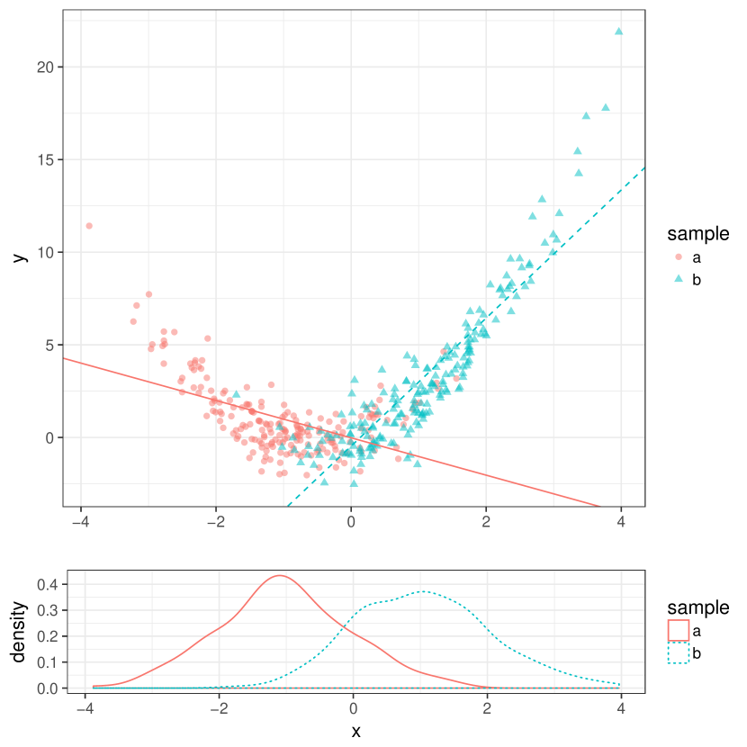
(a) Before matching.

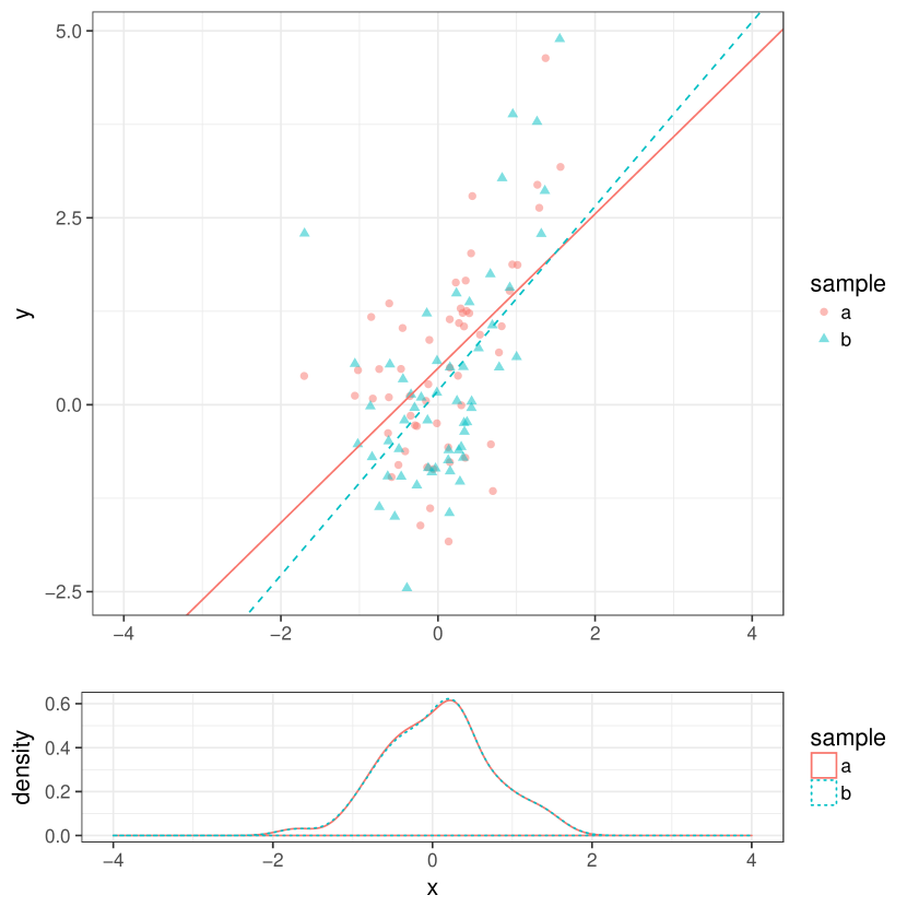
(b) After nearest neighbor matching (pairs are kept if the absolute within pair difference is less than $0.1$).

Figure 1: “Conspiracy” of model misspecification and random design. In this example, $f^{a}(z,v)=f^{b}(z,v)=z^{2}+z+v$ where $v^{a}\overset{d}{=}v^{b}\sim\mathrm{N}(0,1)$, $z^{a}\sim\mathrm{N}(-1,1)$, and $z^{b}\sim\mathrm{N}(1,1)$. If the model is misspecified and a linear model is used as an approximation, $f^{s}(z,v)\approx\eta^{s}+\gamma^{s}z^{s}$, the projections $\gamma^{a}$ and $\gamma^{b}$ depends on the distribution of $z^{a}$ and $z^{b}$ and have different signs in this example. By only considering the common support of the two samples and matching the observations, the projections $\gamma^{a}$ and $\gamma^{b}$ are much closer.

There are two ways to mitigate the issue of non-linearity of the instrument-exposure equation. The first is to only consider the common support of $\mathbf{z}^{a}$ and $\mathbf{z}^{b}$ as suggested by Lawlor (2016) and match or weight the observations so that $\mathbf{z}^{a}$ and $\mathbf{z}^{b}$ have the same distribution. This ensures the projections $\bm{\gamma}^{a}$ and $\bm{\gamma}^{b}$ are the same and is illustrated in Figure 1. The second solution is to nonparametrically model the instrument-exposure relation to avoid the drawback of using the linear approximations. However, this is difficult if the dimension of the IVs is high.

We want to emphasize that, unlike the scenario with linear instrument-exposure equation in Section 3, both solutions above still hinge on sampling invariance of noise variables (Assumption 5). Even if the distributions of $\mathbf{z}^{a}$ and $\mathbf{z}^{b}$ are the same and $f^{a}$ is modeled nonparametrically, the best linear or nonlinear approximation still depends on the distribution of the noise variable $v$. If Assumption 5 is violated so $v^{a}$ and $v^{b}$ have different distributions, the TSIV estimators are still generally biased, though the bias is unlikely to be extremely large. It is also worth noting that sampling homogeneity of the noise variables (Assumption 5) is untestable in the two sample setting because $\mathbf{x}^{b}$ is not observed.

One way to relax Assumption 5 is to assume the instrument-exposure equation is additive:

Assumption 6.

(Additivity of the instrument-exposure equation) $f^{s}(\mathbf{z},v)=f^{s}_{z}(\mathbf{z})+f^{s}_{v}(v)$.

Under Assumption 6, we may non-parametrically estimate $f_{z}^{s}(\mathbf{z})$ and then estimate $\beta^{b}$ by regressing $y_{i}^{b}$ on the predicted $f_{z}^{a}(\mathbf{z}_{i}^{b})$. This is consistent for $\beta^{b}$ if $f_{z}^{a}$ is estimated consistently, because

$$y_{i}^{b}=\beta^{b}x_{i}^{b}+u_{i}^{b}=\beta^{b}f^{b}_{z}(\mathbf{z}_{i}^{b})+\beta^{b}f^{b}_{v}(v_{i}^{b})+u_{i}^{b}=\beta^{b}f^{a}_{z}(\mathbf{z}_{i}^{b})+(\beta^{b}f^{a}_{v}(v_{i}^{b})+u_{i}^{b}).$$

The last equation used structural invariance (Assumption 4). Even if the noise variables $u$ and $v$ may have different distributions in the two samples, the estimation of $\beta^{b}$ is not affected (see Section 4). To summarize, we have shown that

Proposition 2.

In Proposition 1 and absence of noise homogeneity, $\beta^{b}$ can still be identified if the exposure equation is additive.

6 Relaxing linearity of the exposure-outcome equation

6.1 LATE in the one-sample setting

When the exposure-outcome equation is nonlinear, an additional assumption called homogeneity is usually needed to identify the causal effect. Next we review this approach in the one-sample setting when the instrument and the exposure are both binary. In this case, we can define four classes of observations based on the instrument-exposure equation: for $s=a,b$,

$$t^{s}(v)=\begin{cases}\mathrm{always~{}taker~{}(at)},&\mathrm{if}~{}f^{s}(0,v)=1,~{}f^{s}(1,v)=1,\\ \mathrm{complier~{}(co)},&\mathrm{if}~{}f^{s}(0,v)=0,~{}f^{s}(1,v)=1,\\ \mathrm{never~{}taker~{}(nt)},&\mathrm{if}~{}f^{s}(0,v)=0,~{}f^{s}(1,v)=0,\\ \mathrm{defier~{}(de)},&\mathrm{if}~{}f^{s}(0,v)=1,~{}f^{s}(1,v)=0.\\ \end{cases}$$

Classes are important to remove endogeneity since conditioning on the class, the exposure $x$ is no longer dependent on the noise variable $u$, that is

$$x^{s}\mathchoice{\mathrel{\hbox to0.0pt{$\displaystyle\perp$\hss}\mkern 2.0mu{\displaystyle\perp}}}{\mathrel{\hbox to0.0pt{$\textstyle\perp$\hss}\mkern 2.0mu{\textstyle\perp}}}{\mathrel{\hbox to0.0pt{$\scriptstyle\perp$\hss}\mkern 2.0mu{\scriptstyle\perp}}}{\mathrel{\hbox to0.0pt{$\scriptscriptstyle\perp$\hss}\mkern 2.0mu{\scriptscriptstyle\perp}}}u^{s}\,|\,t^{s}(v^{s}).$$ (11)

The last equation is true because given $t^{s}(v^{s})$ and hence the values of $f^{s}(0,v)$ and $f^{s}(1,v)$, the only randomness of $x^{s}$ comes from $z^{s}$ which is independent of $u^{s}$. If the classes were observable, (11) implies that we can identify the class-conditional average outcome $\mathrm{E}[g^{s}(x,u^{s})|t^{s}=t]$ for $(t,x)$ in the support of $(t^{s},x^{s})$, which is a subset of $\{at,co,nt,de\}\times\{0,1\}$. More specifically, since $\mathrm{P}(x^{s}=0|t^{s}=at)=0$ and $\mathrm{P}(x^{s}=1|t^{s}=nt)=0$, the support of $(t^{s},x^{s})$ contains $6$ elements, $\mathrm{supp}(t^{s},x^{s})=\{(at,1),(co,0),(co,1),(nt,0),(de,0),(de,1)\}$. However, the classes are not directly observable, and in fact we can only identify four conditional expectations $\mathrm{E}[y^{s}|x^{s}=x,z^{s}=z]=\mathrm{E}[g^{s}(x,u^{s})|x^{s}=x,z^{s}=z]$ from the data. This means that the class-conditional average outcomes are not identifiable, because in the following system of equations,

$$\begin{split}\mathrm{E}[g^{s}(0,u^{s})|x^{s}=0,z^{s}=0]&=\mathrm{E}[g^{s}(0,u^{s})|t^{s}=nt]\cdot\mathrm{P}(t^{s}=nt)+\mathrm{E}[g^{s}(0,u^{s})|t^{s}=co]\cdot\mathrm{P}(t^{s}=co),\\ \mathrm{E}[g^{s}(0,u^{s})|x^{s}=0,z^{s}=1]&=\mathrm{E}[g^{s}(0,u^{s})|t^{s}=nt]\cdot\mathrm{P}(t^{s}=nt)+\mathrm{E}[g^{s}(0,u^{s})|t^{s}=de]\cdot\mathrm{P}(t^{s}=de),\\ \mathrm{E}[g^{s}(1,u^{s})|x^{s}=1,z^{s}=0]&=\mathrm{E}[g^{s}(1,u^{s})|t^{s}=at]\cdot\mathrm{P}(t^{s}=at)+\mathrm{E}[g^{s}(1,u^{s})|t^{s}=de]\cdot\mathrm{P}(t^{s}=de),\\ \mathrm{E}[g^{s}(1,u^{s})|x^{s}=1,z^{s}=1]&=\mathrm{E}[g^{s}(1,u^{s})|t^{s}=at]\cdot\mathrm{P}(t^{s}=at)+\mathrm{E}[g^{s}(1,u^{s})|t^{s}=co]\cdot\mathrm{P}(t^{s}=co),\end{split}$$ (12)

there are six class-conditional average outcomes but only four equations. Note that to derive (12) we have used Assumption 2 which asserts $z^{s}\mathchoice{\mathrel{\hbox to0.0pt{$\displaystyle\perp$\hss}\mkern 2.0mu{\displaystyle\perp}}}{\mathrel{\hbox to0.0pt{$\textstyle\perp$\hss}\mkern 2.0mu{\textstyle\perp}}}{\mathrel{\hbox to0.0pt{$\scriptstyle\perp$\hss}\mkern 2.0mu{\scriptstyle\perp}}}{\mathrel{\hbox to0.0pt{$\scriptscriptstyle\perp$\hss}\mkern 2.0mu{\scriptscriptstyle\perp}}}t^{s}=t^{s}(v^{s})$ and $z^{s}\mathchoice{\mathrel{\hbox to0.0pt{$\displaystyle\perp$\hss}\mkern 2.0mu{\displaystyle\perp}}}{\mathrel{\hbox to0.0pt{$\textstyle\perp$\hss}\mkern 2.0mu{\textstyle\perp}}}{\mathrel{\hbox to0.0pt{$\scriptstyle\perp$\hss}\mkern 2.0mu{\scriptstyle\perp}}}{\mathrel{\hbox to0.0pt{$\scriptscriptstyle\perp$\hss}\mkern 2.0mu{\scriptscriptstyle\perp}}}u^{s}$, so $\mathrm{E}[g^{s}(x,u^{s})|z^{s},t^{s}]=\mathrm{E}[g^{s}(x,u^{s})|t^{s}]$ and $\mathrm{P}(t^{s}=t|z^{s})=\mathrm{P}(t^{s}=t)$ for any fixed $x$ and $t$.

The monotonicity assumption is used to reduce the number of free parameters in (12).

Assumption 7.

(Monotonicity) $f^{s}(z,v)$ is a monotone function of $z$ for any $v$ and $s=a,b$.

Without loss of generality, we will assume $f^{s}(z,v)$ is an increasing function of $z$, otherwise we can use $-x^{s}=-f^{s}(z^{s},v^{s})$ as the exposure. In the context of binary instrument and binary exposure, Assumption 7 means that $\mathrm{P}(t^{s}=de)=0$ and is often called the no-defiance assumption (Balke and Pearl, 1997). This eliminates two class-conditional average outcomes, $\mathrm{E}[g^{s}(0,u^{s})|t^{s}=de]$ and $\mathrm{E}[g^{s}(1,u^{s})|t^{s}=de]$, leaving us four equations and four class-conditional average outcomes. Therefore, using (12), we can identify the so called local average treatment effect (LATE), $\mathrm{E}[g^{s}(1,u^{s})-g^{s}(0,u^{s})|t^{s}=co]$ (Angrist et al., 1996). In particular, under Assumptions 1, 2 and 7, one can show that the TSLS estimator in sample $s$ converges to

$$\begin{split}\beta_{\mathrm{LATE}}^{s}=&\frac{\mathrm{E}[y^{s}|z^{s}=1]-\mathrm{E}[y^{s}|z^{s}=0]}{\mathrm{E}[x^{s}|z^{s}=1]-\mathrm{E}[x^{s}|z^{s}=0]}\\ =&\frac{\mathrm{E}[g^{s}(1,u^{s})-g^{s}(0,u^{s})|t^{s}=co]\cdot\mathrm{P}(t^{s}=co)}{\mathrm{P}(t^{s}=co)}\\ =&\mathrm{E}[g^{s}(1,u^{s})-g^{s}(0,u^{s})|t^{s}=co].\end{split}$$ (13)

See (14) below for proof this result.

When the exposure $x$ is continuous, we may still define the class $t$ such that (11) holds and identify the class-conditional average outcomes on the joint support of $x$ and $t$. This support may be very limited when the instrument $z$ is binary. We refer the reader to Imbens (2007) for further detail and discussion. In this case, the instrumental variable estimator $\hat{\beta}_{h}$ in (9) converges in probability to a weighted average of local average treatment effects (Angrist et al., 2000). Note that in order for the weights to be non-negative, ordering the instruments by $\mathrm{E}[x^{s}|z^{s}=z]$ must simultaneously order the instruments by the value of $h(z)$ (Angrist et al., 2000, Theorem 2,3). A preferable choice of $h(z)$ is the conditional expectation $\mathrm{E}[x^{s}|z^{s}=z]$.

6.2 LATE in the two-sample setting

We can still follow the LATE framework in the two-sample setting considered in this paper. When the instrument and the exposure are both binary, the TSTSLS estimator converges to a modification of (13) by taking the expectations in the numerator over sample $a$ and the expectations in the denominator over sample $b$,

$$\begin{split}\beta_{\mathrm{LATE}}^{ab}=&\frac{\mathrm{E}[y^{b}|z^{b}=1]-\mathrm{E}[y^{b}|z^{b}=0]}{\mathrm{E}[x^{a}|z^{a}=1]-\mathrm{E}[x^{a}|z^{a}=0]}\\ =&\frac{\mathrm{E}[g^{b}(1,u^{b})-g^{b}(0,u^{b})|t^{b}=co]\cdot\mathrm{P}(t^{b}=co)}{\mathrm{P}(t^{a}=co)}\\ =&\beta_{\mathrm{LATE}}^{b}\cdot\frac{\mathrm{P}(t^{b}=co)}{\mathrm{P}(t^{a}=co)}.\end{split}$$ (14)

Next we prove the second equality in (14). First we consider the numerator

$$\begin{split}&\mathrm{E}[y^{b}|z^{b}=1]-\mathrm{E}[y^{b}|z^{b}=0]\\ =&\sum_{t\in\{at,co,nt,de\}}\big{(}\mathrm{E}[y^{b}|z^{b}=1,t^{b}=t]-\mathrm{E}[y^{b}|z^{b}=0,t^{b}=t]\big{)}\cdot\mathrm{P}(t^{b}=t)\\ =&\sum_{t\in\{at,co,nt\}}\big{(}\mathrm{E}[y^{b}|z^{b}=1,t^{b}=t]-\mathrm{E}[y^{b}|z^{b}=0,t^{b}=t]\big{)}\cdot\mathrm{P}(t^{b}=t)\\ \end{split}$$

where the first equality is due to the law of total expectation and the second equality uses Assumption 7. Next, notice that $y^{b}\mathchoice{\mathrel{\hbox to0.0pt{$\displaystyle\perp$\hss}\mkern 2.0mu{\displaystyle\perp}}}{\mathrel{\hbox to0.0pt{$\textstyle\perp$\hss}\mkern 2.0mu{\textstyle\perp}}}{\mathrel{\hbox to0.0pt{$\scriptstyle\perp$\hss}\mkern 2.0mu{\scriptstyle\perp}}}{\mathrel{\hbox to0.0pt{$\scriptscriptstyle\perp$\hss}\mkern 2.0mu{\scriptscriptstyle\perp}}}z^{b}|t^{b}=at$, because $\mathrm{P}(x^{b}=1|t^{b}=at)=1$ and by the exclusion restriction (implied from Assumption 2), $y^{b}$ only depends on $z^{b}$ through $x^{b}$. Similarly, $y^{b}\mathchoice{\mathrel{\hbox to0.0pt{$\displaystyle\perp$\hss}\mkern 2.0mu{\displaystyle\perp}}}{\mathrel{\hbox to0.0pt{$\textstyle\perp$\hss}\mkern 2.0mu{\textstyle\perp}}}{\mathrel{\hbox to0.0pt{$\scriptstyle\perp$\hss}\mkern 2.0mu{\scriptstyle\perp}}}{\mathrel{\hbox to0.0pt{$\scriptscriptstyle\perp$\hss}\mkern 2.0mu{\scriptscriptstyle\perp}}}z^{b}|t^{b}=ne$. Therefore, we are left with just the compliers

$$\begin{split}&\mathrm{E}[y^{b}|z^{b}=1]-\mathrm{E}[y^{b}|z^{b}=0]\\ =&\big{(}\mathrm{E}[y^{b}|z^{b}=1,t^{b}=co]-\mathrm{E}[y^{b}|z^{b}=0,t^{b}=co]\big{)}\cdot\mathrm{P}(t^{b}=co)\\ =&\big{(}\mathrm{E}[g^{b}(1,u^{b})|z^{b}=1,t^{b}=co]-\mathrm{E}[g^{b}(0,u^{b})|z^{b}=0,t^{b}=co]\big{)}\cdot\mathrm{P}(t^{b}=co)\\ =&\big{(}\mathrm{E}[g^{b}(1,u^{b})|t^{b}=co]-\mathrm{E}[g^{b}(0,u^{b})|t^{b}=co]\big{)}\cdot\mathrm{P}(t^{b}=co).\\ \end{split}$$

In the last equation we have again used the exclusion restriction. Similarly, the denominator in (14) is

$$\begin{split}&\mathrm{E}[x^{b}|z^{b}=1]-\mathrm{E}[x^{b}|z^{b}=0]\\ =&\sum_{t\in\{at,co,nt\}}\big{(}\mathrm{E}[x^{b}|z^{b}=1,t^{b}=t]-\mathrm{E}[x^{b}|z^{b}=0,t^{b}=t]\big{)}\cdot\mathrm{P}(t^{b}=t)\\ =&(1-1)\cdot\mathrm{P}(t^{b}=at)+(1-0)\cdot\mathrm{P}(t^{b}=co)+(0-0)\cdot\mathrm{P}(t^{b}=nt)\\ =&\mathrm{P}(t^{b}=co).\end{split}$$

Finally, note that similar to the one-sample case, (14) only uses Assumptions 1, 2 and 7.

When structural invariance of the instrument-exposure equation $f$ (Assumption 4) and sampling homogeneity of the noise variable $v$ (Assumption 5) hold, we have $t^{a}\overset{d}{=}t^{b}$ because the class $t^{s}$ is a function of $f^{s}$ and $v^{s}$. Therefore $\beta_{\mathrm{LATE}}^{ab}=\beta_{\mathrm{LATE}}^{b}$ by equation (14). To summarize, we have just shown that

Proposition 3.

When there is one binary instrument and one binary exposure, under Assumptions 1, 2, 5 and 7, the TSTSLS estimator identifies $\beta^{b}_{\text{LATE}}$.

In general, the estimand of TSTSLS is a scaling of the LATE in the sample $b$. Since $f^{a}$ and $f^{b}$ are non-trivial functions of $z$ by Assumption 2, the proportions of compliers are positive and hence the ratio $\mathrm{P}(t^{b}=co)/\mathrm{P}(t^{a}=co)>0$. This means that $\beta_{\mathrm{LATE}}^{ab}$ has the same sign as $\beta_{\mathrm{LATE}}^{b}$.

When the exposure is continuous, most of the arguments in Angrist et al. (2000) would still hold as they were proved separately for the numerator and the denominator just like our proof of (14). Similarly, the TSTSLS estimator converges in probability to the estimand of the TSLS estimator in sample $b$ times a scaling factor, and the scaling factor is equal to $1$ under Assumptions 4 and 5. However, the scaling factor is not always positive because in the absence of Assumption 5, the conditional expectation $\mathrm{E}[x^{s}|z^{s}]$ can be different in the two samples (same issue as in Section 5). Similar to Section 5, this can be resolved by assuming additivity (Assumption 6).

7 Simulation

We evaluate the efficiency and robustness of the linear TSIV estimators using numerical simulation. In all simulations we consider $10$ binary instrumental variables generated by

$$\mathbf{z}_{i}^{s}=\mathrm{sign}(\mathbf{z}_{i}^{s*}),~{}\mathbf{z}_{i}^{s*}\overset{i.i.d.}{\sim}\mathrm{N}(\mathbf{1},\bm{\Sigma}^{s}),~{}\Sigma_{jk}^{s}=(\rho^{s})^{|j-k|},~{}s=a,b.$$ (15)

We first verify the asymptotic results regarding the TSIV estimators in Section 3. In our first simulation, the exposures and the outcomes are generated by

$$x_{i}^{s} =0.2\cdot(\mathbf{1}^{T}\mathbf{z}_{i}^{s})+v_{i}^{s},$$ (16)

$$y_{i}^{s} =x_{i}^{s}+u_{i}^{s},$$ (17)

$$(v_{i}^{s},u_{i}^{s}) \overset{i.i.d.}{\sim}\mathrm{N}\left(\begin{pmatrix}0\\ 0\\ \end{pmatrix},\begin{pmatrix}1&\sigma_{uv}\\ \sigma_{uv}&1\\ \end{pmatrix}\right),~{}i=1,\dotsc,n^{s},~{}s=a,b.$$ (18)

In this simulation we used $\rho^{a}=0.5$, $\rho^{b}=0.5$, $0$, or $-0.5$, $n^{a}=1000$ or $5000$, $n^{b}=1000$ or $5000$, and $\sigma_{uv}=0.5$.

In Table 3, we compare the performance of the TSTSLS estimator and the optimal TSIV estimator after centering the variables. In particular, we report the bias, standard deviation (SD), average standard error (SE), and coverage of the 95% asymptotic confidence interval. When $\rho^{a}=\rho^{b}=0.5$, the two estimators are asymptotically equivalent by (7). This is verified by Table 3 as the two estimators have the same bias, variance, and coverage in this case. When $\rho^{a}$ and $\rho^{b}$ are different, the optimal TSIV estimator should be more efficient than TSTSLS (at least theoretically). In the simulations we find that in almost all cases the two estimators have the same variance, but the optimal TSIV estimator has smaller finite sample bias. The difference between the optimal TSIV estimator and the TSTSLS estimator is substantial only if $\bm{\Sigma}^{a}$ and $\bm{\Sigma}^{b}$ (in this simulation, $\rho^{a}$ and $\rho^{b}$) are very different and $n^{b}$ is much larger than $n^{a}$. This phenomenon can also be seen from (7) as discussed in Remark 2.

Table 3: Simulation 1: Asymptotic efficiency of the TSTSLS and optimal TSIV estimators. The reported numbers are obtained by 10000 realizations of data simulated from equations (15), (19), (17), and (18).

					TSTSLS				Optimal TSIV
$\beta$	$\rho^{a}$	$\rho^{b}$	$n^{a}$	$n^{b}$	Bias	SD	SE	Cover	Bias	SD	SE	Cover
1	0.5	0.5	1000	1000	$-0.020$	$0.100$	$0.100$	$0.941$	$-0.020$	$0.100$	$0.100$	$0.941$
				5000	$-0.021$	$0.062$	$0.063$	$0.924$	$-0.021$	$0.062$	$0.063$	$0.923$
			5000	1000	$-0.006$	$0.090$	$0.090$	$0.949$	$-0.006$	$0.090$	$0.090$	$0.949$
				5000	$-0.004$	$0.045$	$0.045$	$0.948$	$-0.004$	$0.045$	$0.045$	$0.948$
		0	1000	1000	$-0.046$	$0.126$	$0.126$	$0.928$	$-0.039$	$0.127$	$0.126$	$0.933$
				5000	$-0.047$	$0.072$	$0.072$	$0.875$	$-0.029$	$0.072$	$0.071$	$0.909$
			5000	1000	$-0.012$	$0.121$	$0.120$	$0.948$	$-0.011$	$0.121$	$0.120$	$0.947$
				5000	$-0.010$	$0.057$	$0.057$	$0.947$	$-0.008$	$0.057$	$0.057$	$0.948$
		-0.5	1000	1000	$-0.058$	$0.135$	$0.135$	$0.918$	$-0.045$	$0.137$	$0.134$	$0.924$
				5000	$-0.058$	$0.077$	$0.075$	$0.851$	$-0.031$	$0.076$	$0.074$	$0.907$
			5000	1000	$-0.012$	$0.130$	$0.129$	$0.951$	$-0.011$	$0.130$	$0.129$	$0.951$
				5000	$-0.013$	$0.060$	$0.061$	$0.947$	$-0.010$	$0.061$	$0.061$	$0.949$
10	0.5	0.5	1000	1000	$-0.197$	$0.726$	$0.726$	$0.929$	$-0.197$	$0.724$	$0.724$	$0.929$
				5000	$-0.194$	$0.548$	$0.548$	$0.915$	$-0.192$	$0.544$	$0.545$	$0.916$
			5000	1000	$-0.036$	$0.577$	$0.578$	$0.949$	$-0.036$	$0.577$	$0.578$	$0.949$
				5000	$-0.037$	$0.327$	$0.327$	$0.948$	$-0.037$	$0.327$	$0.327$	$0.948$
		0	1000	1000	$-0.468$	$0.867$	$0.866$	$0.898$	$-0.330$	$0.870$	$0.860$	$0.920$
				5000	$-0.475$	$0.596$	$0.585$	$0.836$	$-0.249$	$0.587$	$0.574$	$0.900$
			5000	1000	$-0.096$	$0.755$	$0.754$	$0.947$	$-0.086$	$0.756$	$0.753$	$0.948$
				5000	$-0.102$	$0.393$	$0.393$	$0.938$	$-0.072$	$0.394$	$0.392$	$0.941$
		-0.5	1000	1000	$-0.586$	$0.932$	$0.915$	$0.876$	$-0.380$	$0.933$	$0.902$	$0.907$
				5000	$-0.575$	$0.626$	$0.610$	$0.808$	$-0.254$	$0.598$	$0.585$	$0.902$
			5000	1000	$-0.112$	$0.807$	$0.807$	$0.948$	$-0.093$	$0.808$	$0.807$	$0.948$
				5000	$-0.118$	$0.420$	$0.415$	$0.934$	$-0.071$	$0.419$	$0.413$	$0.943$

In the second simulation, we examine how misspecification of the instrument-exposure equation may bias the TSIV estimator. The data are generated in the same way as in the first simulation except that we add interaction terms in the instrument-exposure equation. More specifically, (16) is replaced by

$$x_{i}^{s}=0.2\cdot(\mathbf{1}^{T}\mathbf{z}_{i}^{s})+0.02\cdot\sum_{j\neq k}z_{ij}^{s}z_{ik}^{s}+v_{i}^{s}.$$ (19)

The results of the second simulation are reported in Table 4. When $\rho^{a}=\rho^{b}=0.5$, the TSTSLS and the optimal TSIV estimators are still unbiased and the confidence intervals provide desired coverage. This is because the best linear approximations of the instrument-exposure equation are the same in the two samples. However, when $\rho^{a}\neq\rho^{b}$, the TSTSLS and the optimal TSIV estimators are biased and failed to cover the true parameter at the nominal $95\%$ rate. As discussed in Section 5, this is because the best linear approximations of the instrument-exposure equation are different in the two samples. In addition, note that the optimal TSIV estimator tends to have larger bias in this simulation.

Table 4: Simulation 2: When the instrument-exposure equation is misspecified, the TSIV estimators can be biased. The reported numbers are obtained by 10000 realizations of data simulated from equations (15), (20), (17), and (21).

					TSTSLS				Optimal TSIV
$\beta$	$\rho^{a}$	$\rho^{b}$	$n^{a}$	$n^{b}$	Bias	SD	SE	Cover	Bias	SD	SE	Cover
1	0.5	0.5	1000	1000	$-0.009$	$0.069$	$0.067$	$0.938$	$-0.009$	$0.068$	$0.067$	$0.940$
				5000	$-0.011$	$0.044$	$0.042$	$0.922$	$-0.010$	$0.044$	$0.042$	$0.922$
			5000	1000	$-0.001$	$0.061$	$0.060$	$0.946$	$-0.001$	$0.061$	$0.060$	$0.946$
				5000	$-0.002$	$0.031$	$0.030$	$0.942$	$-0.002$	$0.031$	$0.030$	$0.942$
		0	1000	1000	$\phantom{-}0.041$	$0.086$	$0.085$	$0.927$	$\phantom{-}0.046$	$0.086$	$0.085$	$0.920$
				5000	$\phantom{-}0.042$	$0.051$	$0.050$	$0.878$	$\phantom{-}0.052$	$0.051$	$0.049$	$0.827$
			5000	1000	$\phantom{-}0.059$	$0.081$	$0.080$	$0.885$	$\phantom{-}0.060$	$0.081$	$0.080$	$0.884$
				5000	$\phantom{-}0.060$	$0.039$	$0.038$	$0.665$	$\phantom{-}0.061$	$0.039$	$0.038$	$0.651$
		-0.5	1000	1000	$\phantom{-}0.050$	$0.092$	$0.091$	$0.919$	$\phantom{-}0.059$	$0.093$	$0.091$	$0.904$
				5000	$\phantom{-}0.051$	$0.054$	$0.052$	$0.847$	$\phantom{-}0.067$	$0.054$	$0.052$	$0.755$
			5000	1000	$\phantom{-}0.074$	$0.086$	$0.086$	$0.860$	$\phantom{-}0.075$	$0.086$	$0.086$	$0.859$
				5000	$\phantom{-}0.075$	$0.041$	$0.041$	$0.561$	$\phantom{-}0.077$	$0.041$	$0.041$	$0.535$

Table 5: Simulation 3: Even if the instruments have the same distribution and all other assumptions are met, the TSIV estimators can still be biased if Assumption 5 (sampling homogeneity of noise) is violated. The reported numbers are obtained by 10000 realizations of data simulated from equations (15), (16), (17), and (18).

					TSTSLS				Optimal TSIV
$\beta$	$\rho^{a}$	$\rho^{b}$	$n^{a}$	$n^{b}$	Bias	SD	SE	Cover	Bias	SD	SE	Cover
1	0.5	0.5	1000	1000	$-0.14$	$0.279$	$0.268$	$0.899$	$-0.14$	$0.279$	$0.268$	$0.898$
				5000	$-0.13$	$0.145$	$0.131$	$0.761$	$-0.13$	$0.145$	$0.131$	$0.762$
				20000	$-0.14$	$0.097$	$0.082$	$0.555$	$-0.14$	$0.096$	$0.082$	$0.552$
			5000	1000	$-0.10$	$0.294$	$0.268$	$0.892$	$-0.10$	$0.294$	$0.268$	$0.892$
				5000	$-0.09$	$0.123$	$0.122$	$0.867$	$-0.09$	$0.123$	$0.122$	$0.867$
				20000	$-0.10$	$0.067$	$0.065$	$0.667$	$-0.10$	$0.067$	$0.065$	$0.669$
			20000	1000	$-0.08$	$0.271$	$0.266$	$0.939$	$-0.08$	$0.271$	$0.266$	$0.939$
				5000	$-0.08$	$0.127$	$0.120$	$0.886$	$-0.08$	$0.127$	$0.120$	$0.886$
				20000	$-0.09$	$0.062$	$0.061$	$0.707$	$-0.09$	$0.062$	$0.061$	$0.707$

Even if $\mathbf{z}_{i}^{a}\overset{d}{=}\mathbf{z}_{i}^{b}$, the TSIV estimators can still be biased if $v_{i}^{a}$ and $v_{i}^{b}$ have different distributions and the instrument-exposure equation is not additive (see the discussion after Assumption 6). In our third and final simulation, we generate the data from equations (15) and (17) but replace equations (16) and (18) with

$$x_{i}^{s} =I(0.2\cdot(\mathbf{1}^{T}\mathbf{z}_{i}^{s})+v_{i}^{s}>0),$$ (20)

$$(v_{i}^{s},u_{i}^{s}) \overset{i.i.d.}{\sim}\mathrm{N}\left(\begin{pmatrix}0\\ 0\\ \end{pmatrix},\begin{pmatrix}\sigma_{vv}^{s}&\sigma_{uv}^{s}\\ \sigma_{uv}^{s}&1\\ \end{pmatrix}\right),~{}i=1,\dotsc,n^{s},~{}s=a,b.$$ (21)

In this simulation we use $\rho^{a}=\rho^{b}=0.5$, $\sigma_{vv}^{a}=1$, $\sigma_{vv}^{b}=2$, and $\sigma_{uv}^{s}=0.5\sqrt{\sigma_{vv}^{s}}$, $s=a,b$.

The results of the third simulation are reported in Table 5. Even though $\mathbf{z}_{i}^{a}\overset{d}{=}\mathbf{z}_{i}^{b}$ in this simulation, the TSIV estimators are still biased because the best linear approximations of the instrument-exposure equation depend on the distributions of $v$, which are different in the two samples.

8 Application: The causal effect of body mass index on systolic blood pressure

We apply the one-sample and two-sample IV methods to estimate the causal effect of body mass index (BMI) on systolic blood pressure (SBP) using a real dataset obtained from UK Biobank with 358,928 samples. As benchmarks, we first apply ordinary least squares (OLS) and two IV methods (TSLS and LIML) to the entire dataset with 407 correlated SNPs identified from a previous GWAS of BMI (Locke et al., 2015). The results are reported in the first block in Table 6. The point estimate and confidence interval obtained by OLS are much larger than those obtained by TSLS and LIML, indicating there may be confounding in the observational data. Unsurprisingly, the one-sample IV estimates agree with the two-sample IV estimates using a random 50-50 split (second block in Table 6) and the summary-data MR estimate reported in Zhao et al. (2018) (third block in Table 6).

Next we illustrate the performance of TSIV estimators with heterogeneous samples. Because the UK Biobank population is mostly homogeneous (most of samples are Europeans), we decide to subsample half of the dataset in order to change the distribution of $9$ selected SNPs. This artificially created subsample is then used as the exposure (fourth block in Table 6) or the outcome (fifth block in Table 6), while the other half of the dataset remains unchanged and is used as the other sample in TSIV analyses. We find that the TSIV point estimates using the two heterogeneous samples are different from the benchmarks, though the differences are not statistically significant due to increased standard error. Another observation from Table 6 is that the TSTSLS estimator and the optimal TSIV estimator always give very similar answers. This is not surprising following the discussion in Remark 2.

Table 6: Results of the one-sample and two-sample IV analyses of the UK Biobank data.

Data	# SNPs	Method	Estimate	Standard error	95% CI
One-sample	407	OLS	0.7852	0.0068	[0.7719, 0.7985]
		TSLS	0.4463	0.0366	[0.3746, 0.5180]
		LIML	0.3946	0.0392	[0.3178, 0.4714]
Two-sample (50-50 split)	407	TSTSLS	0.4273	0.0514	[0.3266, 0.5280]
		Optimal TSIV	0.4274	0.0514	[0.3267, 0.5281]
Two-sample (summary data)	160	MR-RAPS (Zhao et al., 2018)	0.4017	0.1063	[0.1934, 0.6100]
Two-sample (subsampled exp.)	9	TSTSLS	0.5199	0.1651	[0.1963, 0.8435]
		Optimal TSIV	0.5210	0.1651	[0.1974, 0.8446]
Two-sample (subsampled out.)	9	TSTSLS	0.6500	0.1975	[0.2629, 1.0371]
		Optimal TSIV	0.6489	0.1975	[0.2618, 1.0360]

9 Summary and discussion

In this paper we have derived a class of linear TSIV estimators when the two samples are heterogeneous. Although the TSTSLS estimator is not asymptotically efficient in general, it usually has great relative efficiency and performs very similarly to the optimal TSIV estimator in the numerical examples. Therefore there is little reason to abandon the already widely-used TSTSLS in practice.

However, when trying to relax the linearity assumption, our theoretical investigation suggests there are additional concerns about using a two-sample IV analysis with heterogeneous samples.

1. Our (in fact any) TSIV analysis can only identify causal effect in the instrument-outcome sample (sample $b$). This is because we do not observe the outcome in sample $a$. This might limit the generalizability of the results of a real study.

2. Compared to the classical one-sample analysis, the TSIV analysis requires additional assumptions to link the two samples. One of the key assumptions is structural invariance (Assumption 4), which might be reasonable in some applications but unreasonable in others (especially if the two populations are drastically different).

3. Another important assumption in the two-sample setting is homogeneity of the distributions of the noise variables (Assumption 5), which is necessary when the exposure equation is not additive. However, this assumption is untestable since we do not observe the exposure variable in one of the samples.

4. Unlike one-sample IV analysis, the heterogeneous two-sample IV analysis generally needs correct specification of the instrument-exposure equation.

Our simulation examples show that violation of any of these three requirements can lead to biased estimates and invalid statistical inference. More real data examples are needed to evaluate the importance of these concerns in practice.

The last point, that is the non-robustness of TSIV to model misspecification and heterogeneous samples, is related to the notion of “invariant prediction” (Peters et al., 2016), “autonomy” (Haavelmo, 1944), or “stability” (Pearl, 2009). These notions are generally stronger as they require invariance of the model under causal interventions. In the problem considered in this paper, we require the exposure predictions are invariant in the two heterogeneous samples. In this view, the structural invariance (Assumption 4) is also not necessary for the identification results. What’s important is the “predictive invariance” in the two samples. In other words, even when Assumption 4 is violated so $f^{a}\neq f^{b}$, the causal effect may still be identifiable if the best linear approximations $\bm{\gamma}^{a}$ and $\bm{\gamma}^{b}$ defined in (10) are the same. We thank an associate editor for pointing out this connection.

References

- 1000 Genomes Project Consortium (2015) 1000 Genomes Project Consortium (2015). A global reference for human genetic variation. Nature 526(7571), 68.
- Abadie (2003) Abadie, A. (2003). Semiparametric instrumental variable estimation of treatment response models. Journal of Econometrics 113(2), 231–263.
- Anderson et al. (1949) Anderson, T. W., H. Rubin, et al. (1949). Estimation of the parameters of a single equation in a complete system of stochastic equations. Annals of Mathematical Statistics 20(1), 46–63.
- Angrist et al. (2000) Angrist, J. D., K. Graddy, and G. W. Imbens (2000). The interpretation of instrumental variables estimators in simultaneous equations models with an application to the demand for fish. Review of Economic Studies 67(3), 499–527.
- Angrist et al. (1996) Angrist, J. D., G. W. Imbens, and D. B. Rubin (1996). Identification of causal effects using instrumental variables. Journal of the American Statistical Association 91(434), 444–455.
- Angrist and Krueger (1992) Angrist, J. D. and A. B. Krueger (1992). The effect of age at school entry on educational attainment: an application of instrumental variables with moments from two samples. Journal of the American Statistical Association 87(418), 328–336.
- Angrist and Krueger (1995) Angrist, J. D. and A. B. Krueger (1995). Split-sample instrumental variables estimates of the return to schooling. Journal of Business & Economic Statistics 13(2), 225–235.
- Baiocchi et al. (2014) Baiocchi, M., J. Cheng, and D. S. Small (2014). Instrumental variable methods for causal inference. Statistics in Medicine 33(13), 2297–2340.
- Baker and Lindeman (1994) Baker, S. G. and K. S. Lindeman (1994). The paired availability design: a proposal for evaluating epidural analgesia during labor. Statistics in Medicine 13(21), 2269–2278.
- Balke and Pearl (1997) Balke, A. and J. Pearl (1997). Bounds on treatment effects from studies with imperfect compliance. Journal of the American Statistical Association 92(439), 1171–1176.
- Barbeira et al. (2016) Barbeira, A., K. P. Shah, J. M. Torres, H. E. Wheeler, E. S. Torstenson, T. Edwards, T. Garcia, G. I. Bell, D. Nicolae, N. J. Cox, et al. (2016). MetaXcan: Summary statistics based gene-level association method infers accurate PrediXcan results. bioRxiv: 045260.
- Bowden et al. (2015) Bowden, J., G. Davey Smith, and S. Burgess (2015). Mendelian randomization with invalid instruments: effect estimation and bias detection through egger regression. International Journal of Epidemiology 44(2), 512–525.
- Bowden et al. (2016) Bowden, J., G. Davey Smith, P. C. Haycock, and S. Burgess (2016). Consistent estimation in mendelian randomization with some invalid instruments using a weighted median estimator. Genetic Epidemiology 40(4), 304–314.
- Buja et al. (2014) Buja, A., R. Berk, L. Brown, E. George, E. Pitkin, M. Traskin, L. Zhao, and K. Zhang (2014). Models as approximations, part i: A conspiracy of nonlinearity and random regressors in linear regression. arXiv:1404.1578.
- Burgess et al. (2015) Burgess, S., R. A. Scott, N. J. Timpson, G. D. Smith, S. G. Thompson, E.-I. Consortium, et al. (2015). Using published data in Mendelian randomization: a blueprint for efficient identification of causal risk factors. European Journal of Epidemiology 30(7), 543–552.
- Burgess et al. (2015) Burgess, S., D. S. Small, and S. G. Thompson (2015). A review of instrumental variable estimators for Mendelian randomization. Statistical Methods in Medical Research.
- Choi et al. (2018) Choi, J., J. Gu, and S. Shen (2018). Weak-instrument robust inference for two-sample instrumental variables regression. Journal of Applied Econometrics 33(1), 109–125.
- Currie and Yelowitz (2000) Currie, J. and A. Yelowitz (2000). Are public housing projects good for kids? Journal of Public Economics 75(1), 99–124.
- Davey Smith and Ebrahim (2003) Davey Smith, G. and S. Ebrahim (2003). “Mendelian randomization”: can genetic epidemiology contribute to understanding environmental determinants of disease? International Journal of Epidemiology 32(1), 1–22.
- Davey Smith and Hemani (2014) Davey Smith, G. and G. Hemani (2014). Mendelian randomization: genetic anchors for causal inference in epidemiological studies. Human Molecular Genetics 23(R1), R89–98.
- Davidson and MacKinnon (1993) Davidson, R. and J. G. MacKinnon (1993). Estimation and inference in econometrics. Oxford University Press.
- Fuller (1977) Fuller, W. A. (1977). Some properties of a modification of the limited information estimator. Econometrica, 939–953.
- Gamazon et al. (2015) Gamazon, E. R., H. E. Wheeler, K. P. Shah, S. V. Mozaffari, K. Aquino-Michaels, R. J. Carroll, A. E. Eyler, J. C. Denny, D. L. Nicolae, N. J. Cox, et al. (2015). A gene-based association method for mapping traits using reference transcriptome data. Nature Genetics 47(9), 1091–1098.
- Graham et al. (2016) Graham, B. S., C. C. d. X. Pinto, and D. Egel (2016). Efficient estimation of data combination models by the method of auxiliary-to-study tilting (ast). Journal of Business & Economic Statistics 34(2), 288–301.
- Haavelmo (1944) Haavelmo, T. (1944). The probability approach in econometrics. Econometrica: Journal of the Econometric Society 12, S1–S115.
- Hansen et al. (2008) Hansen, C., J. Hausman, and W. Newey (2008). Estimation with many instrumental variables. Journal of Business & Economic Statistics 26(4), 398–422.
- Hansen (1982) Hansen, L. P. (1982). Large sample properties of generalized method of moments estimators. Econometrica 50(4), 1029–1054.
- Hemani et al. (2018) Hemani, G., J. Zheng, B. Elsworth, K. H. Wade, V. Haberland, D. Baird, C. Laurin, S. Burgess, J. Bowden, R. Langdon, et al. (2018). The mr-base platform supports systematic causal inference across the human phenome. eLife 7, e34408.
- Hernán and Robins (2006) Hernán, M. A. and J. M. Robins (2006). Instruments for causal inference: an epidemiologist’s dream? Epidemiology, 360–372.
- Imbens and Angrist (1994) Imbens, G. and J. Angrist (1994). Identification and estimation of local average treatment effects. Econometrica 62, 467–475.
- Imbens (2007) Imbens, G. W. (2007). Nonadditive models with endogenous regressors. In R. Blundell, W. Newey, and T. Persson (Eds.), Advances in Economics and Econometrics, Volume 3, pp. 17—46. Cambridge University Press.
- Inoue and Solon (2010) Inoue, A. and G. Solon (2010). Two-sample instrumental variables estimators. The Review of Economics and Statistics 92(3), 557–561.
- Jappelli et al. (1998) Jappelli, T., J.-S. Pischke, and N. S. Souleles (1998). Testing for liquidity constraints in Euler equations with complementary data sources. Review of Economics and Statistics 80(2), 251–262.
- Kang et al. (2016) Kang, H., A. Zhang, T. T. Cai, and D. S. Small (2016). Instrumental variables estimation with some invalid instruments and its application to mendelian randomization. Journal of American Statistical Association 111(513), 132–144.
- Klevmarken (1982) Klevmarken, A. (1982, April). Missing Variables and Two-Stage Least-Squares Estimation from More than One Data Set. Working Paper Series 62, Research Institute of Industrial Economics.
- Lawlor (2016) Lawlor, D. A. (2016). Commentary: Two-sample Mendelian randomization: opportunities and challenges. International Journal of Epidemiology 45(3), 908.
- Lawlor et al. (2008) Lawlor, D. A., R. M. Harbord, J. A. Sterne, N. Timpson, and G. Davey Smith (2008). Mendelian randomization: using genes as instruments for making causal inferences in epidemiology. Statistics in Medicine 27(8), 1133–1163.
- Locke et al. (2015) Locke, A. E., B. Kahali, S. I. Berndt, A. E. Justice, T. H. Pers, F. R. Day, C. Powell, S. Vedantam, M. L. Buchkovich, J. Yang, et al. (2015). Genetic studies of body mass index yield new insights for obesity biology. Nature 518(7538), 197–206.
- Machiela and Chanock (2015) Machiela, M. J. and S. J. Chanock (2015). Ldlink: a web-based application for exploring population-specific haplotype structure and linking correlated alleles of possible functional variants. Bioinformatics 31(21), 3555–3557.
- Manolio et al. (2009) Manolio, T. A., F. S. Collins, N. J. Cox, D. B. Goldstein, L. A. Hindorff, D. J. Hunter, M. I. McCarthy, E. M. Ramos, L. R. Cardon, A. Chakravarti, et al. (2009). Finding the missing heritability of complex diseases. Nature 461, 747–753.
- Ogburn et al. (2015) Ogburn, E. L., A. Rotnitzky, and J. M. Robins (2015). Doubly robust estimation of the local average treatment effect curve. Journal of the Royal Statistical Society: Series B (Statistical Methodology) 77(2), 373–396.
- Pacini (2018) Pacini, D. (2018). The two-sample linear regression model with interval-censored covariates.
- Pacini and Windmeijer (2016) Pacini, D. and F. Windmeijer (2016). Robust inference for the two-sample 2SLS estimator. Economics Letters 146, 50–54.
- Pearl (2009) Pearl, J. (2009). Causality. Cambridge University Press.
- Peters et al. (2016) Peters, J., P. Bühlmann, and N. Meinshausen (2016). Causal inference by using invariant prediction: identification and confidence intervals (with discussion). Journal of the Royal Statistical Society: Series B (Statistical Methodology) 78(5), 947–1012.
- Pierce and Burgess (2013) Pierce, B. L. and S. Burgess (2013). Efficient design for Mendelian randomization studies: subsample and 2-sample instrumental variable estimators. American Journal of Epidemiology 178(7), 1177–1184.
- Ridder and Moffitt (2007) Ridder, G. and R. Moffitt (2007). The econometrics of data combination. Handbook of Econometrics 6, 5469–5547.
- Sherry et al. (2001) Sherry, S. T., M.-H. Ward, M. Kholodov, J. Baker, L. Phan, E. M. Smigielski, and K. Sirotkin (2001). dbsnp: the ncbi database of genetic variation. Nucleic Acids Research 29(1), 308–311.
- Stock et al. (2002) Stock, J. H., J. H. Wright, and M. Yogo (2002). A survey of weak instruments and weak identification in generalized method of moments. Journal of Business & Economic Statistics 20(4), 518–529.
- Theil (1958) Theil, H. (1958). Economic forecasts and policy.
- Vansteelandt and Didelez (2015) Vansteelandt, S. and V. Didelez (2015). Robustness and efficiency of covariate adjusted linear instrumental variable estimators. arXiv preprint arXiv:1510.01770.
- Wald (1940) Wald, A. (1940). The fitting of straight lines if both variables are subject to error. Annals of Mathematical Statistics 11(3), 284–300.
- Wang and Tchetgen Tchetgen (2018) Wang, L. and E. Tchetgen Tchetgen (2018). Bounded, efficient and multiply robust estimation of average treatment effects using instrumental variables. Journal of the Royal Statistical Society: Series B (Statistical Methodology) 80(3), 531–550.
- White (1980) White, H. (1980). Using least squares to approximate unknown regression functions. International Economic Review 21(1), 149–170.
- Wright (1928) Wright, P. G. (1928). Tariff on Animal and Vegetable Oils. Macmillan Company, New York.
- Yang et al. (2012) Yang, J., T. Ferreira, A. P. Morris, S. E. Medland, P. A. Madden, A. C. Heath, N. G. Martin, G. W. Montgomery, M. N. Weedon, R. J. Loos, et al. (2012). Conditional and joint multiple-snp analysis of GWAS summary statistics identifies additional variants influencing complex traits. Nature Genetics 44(4), 369–375.
- Zhao et al. (2018) Zhao, Q., J. Wang, J. Bowden, and D. S. Small (2018). Statistical inference in two-sample summary-data mendelian randomization using robust adjusted profile score. arXiv preprint arXiv:1801.09652.