Nonlinear plasma waves driven by short ultrarelativistic electron bunches

Abstract

We advance a theory of quasistatic approximation and investigate the excitation of nonlinear plasma waves by the driving beam of ultrarelativistic electrons using novel electrostatic-like particle-in-cell code. Assuming that the beam occupies an infinitesimally small volume, we find the radius and length of the plasma bubble formed in the wake of the driver for varying values of the beam charge. The mechanism of the bubble formation is explained by developing simple models of the bubble at large charges. Plasma electrons expelled by the driver charge excite secondary plasma waves which complicate the plasma electron flow near the bubble boundary.

I Introduction

Plasma-based accelerators are capable of producing much higher accelerating gradients than conventional radio frequency accelerating structures. In a plasma wakefield accelerator (PWA) an electron bunch  Chen_1985 ; Tajima_1979 drives a plasma wave propagating with phase velocity $v_{ph}\sim c$, where $c$ is the speed of light. This wave can create a wakefield accelerating gradient $E\sim\sqrt{n_{0}[cm^{-3}]}V/cm$, where $n_{0}$ is the density of plasma electrons. Recent experiments have demonstrated rapid wakefield acceleration of electrons to very high energies blumenfeld_energy_2007 in the strongly nonlinear ‘plasma bubble’ regime Rosenzweig_1991 with plasma electrons fully expelled from the wake of the driving beam.

Particle-in-cell (PIC) simulations fonseca_osiris_2002 ; Pukhov_code ; Nieter_2004 is an indispensable tool for studying interaction of the driving beam with plasma electrons, formation of the plasma bubble and acceleration of the witness beam by the bubble fields. When the driver velocity $v_{dr}\rightarrow c$, the description of the plasma response and the evolution of electromagnetic fields can be significantly simplified under the so called quasistatic approximation Sprangle_1990 ; Mora_1997 . This approximation is a powerful approach laying the foundation for a number of quasistatic codes Mora_1997 ; lotov_fine__2003 ; Huang_QUICK_2006 as well as simplified analytical models Kostyukov_phenomenological_2004 ; Lu_theory_2006 ; Yi_Analytic_2013 . However the equation for the magnetic field involves time derivatives, and therefore is not completely quasistatic. This deficiency complicates its numerical implementation and the overall physical picture.

The excitation of nonlinear plasma waves by an infinitesimally short driver of finite radius has been considered by Barov et al. barov_energy_2004 , and the momentum kick experienced by plasma electrons from the passing driver has been found analytically. Further simplification of the driver has been considered in Ref. stupakov_wake_2016 , where the beam radius is assumed to be the infinitesimally small. Such a ‘point-like’ beam of ultrarelativistic electrons is characterized by only one quantity - its normalized charge

$$Q=\frac{k_{p}^{3}q}{4\pi en_{0}},$$ (1)

where q is the beam charge, $k_{p}\equiv\omega_{p}/c$, $\omega_{p}=(4\pi e^{2}n_{0}/m)^{1/2}$ is the electron plasma frequency, and $c$ is the speed of light. It turns out that in the $Q\rightarrow 0$ limit the shape of the plasma bubble can be found analytically.

Beyond the pointlike beam approximation, an analytical model developed by Lu et al. Lu_theory_2006 predicts that the plasma bubble in the wake of the electron beam resembles a sphere at $Q\gg 1$. This model involves an assumption that the bubble boundary can be approximated by the trajectory of a single plasma electron. It is however unclear whether this approximation is justified for a point-like driver.

As we will see below, the pointlike driver with $Q\gg 1$ kicks plasma electrons at relatively small distances from the driver $r\sim k_{p}^{-1}$. Yet, the size of the plasma bubble observed in simulations Rosenzweig_2004 is much larger than $k_{p}^{-1}$. This discrepancy and underlying physics mechanism of the bubble formation are explained in the present paper.

We use the Vlasov equation for the electron distribution function under quasistatic approximation to describe the plasma response to the self-consistent electromagnetic field in the wake. We derive the quasistatic equations for electromagnetic fields, which do not involve time derivatives in the source terms. Thus, the problem is treated in the similar way as the electrostatic one Birdsall_book .

We incorporate the quasistatic approximation in a novel particle-in-cell (PIC) code. We investigate nonlinear plasma waves in the wake of the pointlike driver and find the radius and length of the plasma bubble for arbitrary values of the driver charge $Q$. We also develop phenomenological models for the plasma bubble in the $Q\gg 1$ limit and compare them with models Kostyukov_phenomenological_2004 ; Lu_theory_2006 .

The rest of the paper is organized as follows. In Sec. II we present the basic equations for the quasi-static theory. The main result of this section is the derivation of the Helmholtz-type equation for magnetic field, with a source term depending only on radial positions and momenta of the plasma electrons. This equation is used in Sec. III to find the initial momentum kick from the driver. We then discuss the wakefield in a ballistic regime (Sec. IV), and present results of the particle-in-cell simulations (Sec. V). In Section VI, we suggest simple models of the plasma bubble behind a large charge driver. These models capture essential features observed in PIC simulations. Finally, we summarize our findings in Sec. VII.

II Equations of quasistatic approximation.

This Section addresses the dynamics of plasma electrons behind a pointlike ultrarelativistic electron beam propagating along a positive direction of the $z$-axis in a cold homogeneous plasma. We adopt a quasistatic approximation by assuming that the driver velocity is equal to the speed of light.

In what following, we use dimensionless units normalizing time to $\omega_{p}^{-1}$, length to $k_{p}^{-1}$, and velocities to $c$. We also normalize the electron kinetic momentum ${\bf{p}}$ to $mc$, the fields ${\bf{E}}$ and ${\bf{B}}$ to $mc\omega_{p}/e$, the potentials $\phi$ and A to $mc^{2}/e$, the plasma density to $n_{0}$, and the current density ${\bf{j}}$ to $-en_{0}c$. In dimensionless units, the current and charge densities of the electron beam are given by

$$j_{dr}=\rho_{dr}=2(Q/r_{\perp})\delta(r_{\perp})\delta(t-z),$$ (2)

where $r=\sqrt{x^{2}+y^{2}}$.

The 3-dimensional motion of plasma electrons in the wake of the driver depends on a single dimensionless parameter $Q$, and is adequately described by the Vlasov kinetic equation for the electron distribution function $f_{e}$ complemented by Maxwell’s equations. We describe this motion under two assumptions: (I) the distribution function $f_{e}$ and electromagnetic fields depend on $t$ and $z$ only through a combination $\xi=t-z$, and (II) the motion is axially symmetric.

First, we simplify the kinetic equation

$$\frac{\partial{f}_{e}}{\partial t}+\frac{\partial H}{\partial{\bf{P}}}\cdot\frac{\partial f_{e}}{\partial{\bf{R}}}-\frac{\partial H}{\partial{\bf{R}}}\cdot\frac{\partial f_{e}}{\partial{\bf{P}}}=0,$$ (3)

where $H=[1+({\bf{P}}+{\bf{A}})^{2}]^{1/2}-\phi$ is the Hamiltonian ${\bf{P}}={\bf{p}}-{\bf{A}}$ is the canonical momentum, $\phi$ is the electric potential, and ${\bf{R}}=(x,y,z)$ is the electron radius vector. The trajectory of an individual electron in phase space $({\bf{R}},{\bf{P}})$ is determined by the equations of motion:

$$\frac{d{\bf{P}}}{dt}=-\frac{\partial H}{\partial{\bf{R}}},\quad\frac{d{\bf{R}}}{dt}=\frac{\partial H}{\partial{\bf{P}}}.$$ (4)

From the dependence of $H$ on $\xi=t-z$, we derive that $dH/dt={\partial H}/{\partial t}={\partial H}/{\partial\xi}$ and $dP_{z}/dt=-{\partial H}/{\partial z}={\partial H}/{\partial\xi}$. Hence, $H-P_{z}=const$. Due to cylindrical symmetry, the Hamiltonian $H$ does not depend on the azimuthal angle $\theta$, so that $d{{P}}_{\theta}/dt={\partial H}/{\partial\theta}=0$. Hence, the azimuthal momentum ${{P}}_{\theta}=const$. Since all electrons start their motion from cold homogenous plasma where $H=1$ and ${\bf{P}}=0$, these integrals of motion take the form:

$$H-P_{z}-1=0,\quad P_{\theta}=0.$$ (5)

In the cylindrical coordinates $(r,\theta,z)$, there are two non-vanishing components of the electric field ($E_{r}$ and $E_{z}$), and one non-vanishing component of the magnetic field ($B_{\theta}$). Using the gauge ${\bf{A}}_{\perp}=0$, we express the magnetic field as $B_{\theta}=-\partial A_{z}/\partial r$ and the transverse components of canonical momentum as ${{P}}_{\theta}={{p}}_{\theta}=xp_{y}-yp_{x}$ and $P_{r}=p_{r}=(xp_{x}+yp_{y})/r$.

Using assumptions (I) and (II) and conservations laws (5), the distribution function of electrons can be expressed in the form

$$f_{e}(t,{\bf{R}},{\bf{P}})=rf_{*}(\xi,{{r}},{{P}}_{r})\delta(H-P_{z}-1)\delta(P_{\theta}),$$ (6)

where $f_{*}$ represent a distribution function of macroparticles performing one dimensional radial motion; the factor $r$ in front of $f_{*}$ is introduced to take into account the particle weight in the cylindrical coordinates, and the variable $\xi$ plays now a role of a new ‘time’. Substituting Eq. (6) into (3), we find that $f_{*}$ satisfies the one-dimensional Vlasov equation (see Appendix A):

$$\frac{\partial}{\partial\xi}{f_{*}}+\frac{\partial H_{*}}{\partial{{p}}_{r}}\frac{1}{r}\frac{\partial}{\partial{{r}}}(rf_{*})-\frac{\partial H_{*}}{\partial{{r}}}\frac{\partial}{\partial{{p}}_{r}}f_{*}=0,$$ (7)

where

$$H_{*}(\xi,r,p_{r})=\frac{1+{{p}}_{r}^{2}+(1+\psi)^{2}}{2(1+\psi)}-\psi-A_{z}$$ (8)

is the Hamiltonian for cylindrically symmetric motion Mora_1997 . This Hamiltonian depends on $\xi$ and $r$ through the wakefield potential $\psi\equiv\phi-A_{z}$ and the vector potential $A_{z}$. The trajectory of an individual particle in the phase space $(r,p_{r})$ is determined by equations of motion

$$\frac{d}{d\xi}{p}_{r}=\frac{\gamma}{1+\psi}\frac{\partial}{\partial r}\psi-B_{\theta},\quad\frac{d}{d\xi}r=V(\xi,r,p_{r}),$$ (9)

where $\gamma=[{1+{{p}}_{r}^{2}+(1+\psi)^{2}}]/{2(1+\psi)}$ is the relativistic factor, and $V\equiv{p_{r}}/({1+\psi})$ is the particle ‘velocity’ in $r$-direction.

Integration of Eq. (7) over momentum $p_{r}$ gives the continuity equation:

$$\frac{\partial}{\partial\xi}n_{*}=-\frac{1}{r}\frac{\partial}{\partial{{r}}}r{{n}}_{*}\langle V\rangle,$$ (10)

where $n_{*}=\int d{{p}}_{r}f_{*}$ is the density of macroparticles, and the brackets denote averaging over transverse momentum $\langle V\rangle={{n}}_{*}^{-1}\int d{{p}}_{r}f_{*}V$. As seen from Eq. (10) that the total number of macroparticles is the same at each $\xi=const$ slice.

In addition to conservation of macroparticles, the total energy of macroparticles is conserved (see Appendix B and Ref. Mora_1997 ). For the point-like driver, this additional conservation law has the form

$$2\pi\int_{0}^{\infty}rdr\bigg{[}n_{*}\langle\gamma-1\rangle+\frac{E_{z}^{2}+(\partial\psi/\partial r)^{2}}{2}\bigg{]}=const.$$ (11)

We also note that the density and the current density of plasma electrons can be expressed through the distribution function $f_{*}$ as:

$$n_{e}=\frac{n_{*}\langle\gamma\rangle}{1+\psi},\quad j_{r}=n_{*}\langle V\rangle,\quad j_{z}=\frac{n_{*}\langle p_{z}\rangle}{1+\psi},$$ (12)

where $\langle p_{z}\rangle=\langle\gamma\rangle-\psi-1=[1+\langle p_{r}^{2}\rangle-(1+\psi)^{2}]/(2(1+\psi)$. Besides, $n_{e}-j_{z}=n_{*}$.

We now show that the wakefield potential $\psi$ and the electric field $E_{z}$ at a ‘time’ $\xi$ are determined only by positions and momenta of macroparticles at the same time, that is, by $f_{*}(\xi,r,p_{r})$. Using $\xi$ as a time-like variable, Maxwell’s equations in dimensionless variables take the following form:

$$\nabla\times{\bf{E}}=-\frac{\partial}{\partial\xi}{\bf{B}},$$ (13)

$$\nabla\times{\bf{B}}=\frac{\partial}{\partial\xi}{\bf{E}}-{\bf{j}}.$$ (14)

We find from Eq. (13) that $E_{r}=-\partial\psi/\partial r+B_{\theta}$ and $E_{z}=\partial\psi/\partial\xi$ in the axially symmetric problem. Substituting these expressions into Gauss’s law $\nabla\cdot{\bf{E}}=-n_{e}+1$ and using Eq. (14), we find the following equations:

$$\frac{1}{r}\frac{\partial}{\partial r}r\frac{\partial}{\partial r}\psi=n_{*}-1,\quad\frac{\partial}{\partial r}E_{z}=-n_{*}\langle V\rangle.$$ (15)

Their solution must satisfy the following boundary condition: $\psi\rightarrow 0$ and $E_{z}\rightarrow 0$ at $r\rightarrow\infty$. Note that the source term $n_{*}-1$ in equation for $\psi$ is fully determined by macroparticles’ positions while the source term $n_{*}\langle V\rangle$ in equation for $E_{z}$ requires knowledge of the macroparticles’ positions and momenta.

Taking a curl of the both sides of Eq. (14) and replacing $\nabla\times{\bf{E}}$ by $-\partial{\bf{B}}/\partial\xi$, we find an equation for the magnetic field $\Delta_{\perp}{\bf{B}}=\nabla\times{\bf{j}}$. Its angular component has the following form:

$$\frac{\partial}{\partial r}\frac{1}{r}\frac{\partial}{\partial r}r{{B}}_{\theta}=-\frac{\partial}{\partial r}j_{z}-\frac{\partial}{\partial\xi}j_{r},$$ (16)

where $j_{z}$ and $j_{r}$ are defined by Eq. (53). To obtain a closed form of the equation for magnetic field, we establish a relationship between the time derivative of the transverse current and the electromagnetic fields. Such a relationship is well-known for cold weakly perturbed plasma Keinigs_1986 : $\partial{\bf{j}}/\partial t=(\omega_{p}^{2}/4\pi){\bf{E}}$. To generalize it to strongly perturbed relativistic plasma, we multiply Eq. (7) by the ’velocity’ ${{V}}=\partial H_{*}(\xi,r,p_{r})/\partial{p_{r}}$ and integrate it over momentum $p_{r}$. After straightforward calculations we obtain

$$\frac{\partial}{\partial\xi}{{j}}_{r}=n_{*}\langle{{a}}\rangle-\frac{1}{r}\frac{\partial}{\partial r}rn_{*}\langle V^{2}\rangle\rangle,$$ (17)

where $a\equiv{d^{2}r}/{d\xi^{2}}$ is the particle ’acceleration’:

$${{a}}=-\frac{B_{\theta}}{1+\psi}+\tilde{a},$$ (18)

$$\tilde{a}=\frac{\gamma}{(1+\psi)^{2}}\frac{\partial\psi}{\partial r}-\frac{{{V}}}{1+\psi}\bigg{(}E_{z}+V\frac{\partial\psi}{\partial{{r}}}\bigg{)}.$$ (19)

We herein define $\tilde{a}$ as a part of ‘acceleration’ caused by the wakefield potential $\psi$ and $E_{z}$. Finally, substituting Eqs. (17) - (19) into Eq. (16) we find that the magnetic field satisfies the Helmholtz equation

$$\frac{\partial}{\partial r}\frac{1}{r}\frac{\partial}{\partial r}rB_{\theta}=\frac{n_{*}}{1+\psi}B_{\theta}-S,$$ (20)

where $S$ is the ‘source’ term

$$S=n_{*}\langle\tilde{a}\rangle+\frac{1}{r}\frac{\partial}{\partial r}rn_{*}\langle V^{2}\rangle+\frac{\partial}{\partial r}j_{z}.$$ (21)

Equation (20) needs to be solved with the boundary conditions $B_{\theta}\rightarrow 0$ at $r\rightarrow\infty$ and $B_{\theta}\rightarrow 0$ at $r\rightarrow 0$.

Shielding of the magnetic field by plasma is clearly seen from Eq. (20). Indeed, the coefficient in front of the first term on the right-hand side of this equation is proportional to $\delta_{s}^{-2}$, where $\delta_{s}$ is the skin depth of relativistic plasma. In dimensional variables,

$$k_{p}^{2}\frac{n_{*}}{1+\psi}=\frac{4\pi e^{2}n_{e}}{m\langle\gamma\rangle c^{2}}=\frac{1}{\delta_{s}^{2}}.$$ (22)

In quasi-static approximation all fields are determined from static Eqs. (15) and (20) by positions $r$ and momenta $p_{r}$ of macroparticles at given ‘time’ $\xi$. The source terms in these equations do not have ‘time’ derivatives of the fields or currents.

III Initial condition for distribution function

In this section we derive the initial kick from the driver experienced by plasma electrons.

The ultrarelativistic driver (45) does not change the density $n_{*}$ because $n_{dr}-j_{dr}=0$. The driver is included in quasi-static equations by replacing $j_{z}\rightarrow j_{z}+j_{dr}$ in Eq. (21). Since $j_{dr}\propto\delta(\xi)$, the $r$-coordinates of macroparticles and their density do not change during short interaction with the driver fields barov_energy_2004 . Therefore, $n_{*}|_{\xi=0+}=n_{*}|_{\xi=0-}=1$ and $\psi|_{\xi=0+}=0$. From Eqs. (20) and (21), we conclude that $B_{\theta}\propto\delta(\xi)$. It follows from Eqs. (9) that momentum $p_{r}$ changes by a finite quantity during short ‘time’ $\xi-0$ to $\xi+0$. Omitting finite terms in the source (21), we transform Eq. (20) in the vicinity of the point $\xi=0$ to the Helmholtz equation with constant coefficients:

$$\frac{\partial}{\partial r}\frac{1}{r}\frac{\partial}{\partial r}rB_{\theta}=B_{\theta}-\frac{\partial}{\partial r}j_{dr}.$$ (23)

The solution of this equation $B_{\theta}=-2QK_{1}(r)\delta(\xi)$, where $K_{1}(r)$ is the modified Bessel function of the second kind, determines the initial transverse momentum as a function of $r$:

$$p_{r}|_{\xi=0+}=2QK_{1}(r).$$ (24)

The corresponding initial distribution function is: $f_{*}|_{\xi=0+}=\delta[p_{r}-2QK_{1}(r)]$. Note that the initial ‘time’ derivative of $\psi$ does not vanish $E_{z}|_{\xi=0+}=2QK_{0}(r)$, although $\psi|_{\xi=0+}=0$. The initial longitudinal momentum and relativistic factor are

$$p_{z}|_{\xi=0+}=\gamma|_{\xi=0+}-1=\frac{1}{2}[2QK_{1}(r)]^{2}.$$ (25)

The initial density of plasma electrons $n_{e}|_{\xi=0+}=\gamma|_{\xi=0+}=1+\frac{1}{2}[2QK_{1}(r)]^{2}$ is apparently singular at $r=0$, but it turns out that this singularity does not affect the characteristics of the plasma flow at $\xi>0$.

IV Ballistic regime

Ballistic regime takes place during the initial stage of the plasma bubble formation ($\xi\ll 1$), when electromagnetic fields generated by plasma charges and currents do not yet affect the motion of the plasma electrons. These electrons move with constant velocity ($dp_{r}/d\xi=0$ and $dr/d\xi=p_{r}$) vacating the area close to axis of the driver propagation. The ballistic trajectory $r=r(\xi)$ starting from the initial position $r_{0}$ is a straight line in the plane $(\xi,r)$ determined by

$$r=r_{0}+2QK_{1}(r_{0})\xi.$$ (26)

The condition $dr_{0}/dr=0$ determines the envelope of these trajectories by the following parametric equations:

$$r_{bal}=r_{0}-K_{1}(r_{0})/K_{1}^{\prime}(r_{0}),$$ (27)

$$\xi=-1/[2QK_{1}^{\prime}(r_{0})],$$ (28)

where $r_{0}$ plays a role of an independent parameter. Note that envelopes at different $Q$ can be obtained from each other by rescaling the axis $\xi$. At small $\xi$, the envelope radius scales as $r\propto\xi^{1/2}$ while at large $\xi$ the radius changes logarithmically $r\sim\ln\xi$.

This envelope creates a boundary of the fully evacuated area: $0<\xi$, $r<r_{bal}(\xi)$. One could expect that electromagnetic fields excited during plasma electron motion should obstruct this motion, rendering plasma bubbles of smaller radii: $r_{b}(\xi)<r_{bal}(\xi)$. However, we find that this is not the case at large $Q$.

V PIC simulations of the electron plasma flow

Based on quasi-static approximation, we have developed in-house particle-in-cell (PIC) code that is similar to an electrostatic PIC code Birdsall_book : We define a grid that divides the radial simulation domain $(0,R_{\max})$, where $R_{\max}\sim 100-300$, into a set of small cells with size $\Delta r\sim 0.02$.

Assuming that positions and momenta of macroparticles are known at the ‘moment’ $\xi$, we calculate the the macroparticle density in each cell, solve Eq. (15), and determine $\psi$. After that we calculate the average ‘velocity’ in each cell $\langle V\rangle=\langle p_{r}\rangle/(1+\psi)$ and then find $E_{z}$. After calculating $\langle V^{2}\rangle=\langle p_{r}^{2}\rangle/(1+\psi)^{2}$ and $S$, we solve Eq. (20) and find $B_{\theta}$. To avoid accumulation of round-off errors, we solve the Helmholtz equation for magnetic field by the method of Gaussian elimination with partial pivoting burden_numerical_2015 . After finding fields $\psi$, $\partial\psi/\partial r$, and $B_{\theta}$, we use Eqs. (9) to push macroparticles to the next ‘moment’ $\xi+\Delta\xi$, where $\Delta\xi$ is the ‘time’ step that can be chosen by physical requirements at each moment $\xi$. We use the adaptive Runge-Kutta method for the ‘time’ integration, and vary the ’time’ step $\Delta\xi$ to accurately reproduce the frontal and rear parts of the plasma bubble where the bubble boundaries are steep.

V.1 Comparison of plasma bubbles at small and large driver charges

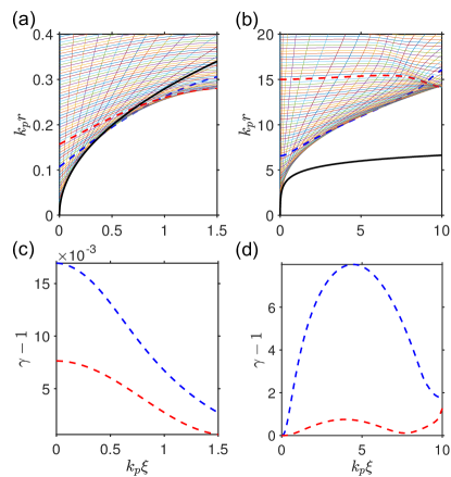
Figure 1: Trajectories of electrons near the frontal part of the plasma bubble obtained from quasistatic PIC simulations: (a) $Q=0.01$ and (b) $Q=25$. Blue and red dashed curves denote representative trajectories touching the bubble boundary at different points. Panels (c) Q=0.01 and (d) Q=25 show change of the particle energy along these trajectories. Black curves are the envelopes of ballistic trajectories determined by Eqs. (27) and (28). The driver is located at the point $(\xi,r)=(0,0)$.

It is instructive to compare the plasma bubbles at small and large values of $Q$. Figure 1 shows trajectories of particles near the frontal part of the bubble at $Q=0.01$ and $Q=25$. It also shows the envelopes of the ballistic trajectories.

When the driver charge is small, the electron velocities in the vicinity of the bubble are also small ($v_{r}\sim 2Q/r\ll 1$ and $v_{z}\approx v_{r}^{2}/2\ll v_{r}$). The magnetic field can therefore be neglected, so that the electrons experience only attraction to the axis by the bubble ions, a force proportional to $\partial_{r}\psi$. One can find then the transverse bubble radius $r_{\max}$ from simple estimates. During particle motion, its initial kinetic energy $T\sim(2Q/r)^{2}/2$ is transformed to the potential energy of this particle $U\sim\frac{1}{4}r^{2}$ at the point where the radius of the bubble reaches maximum value $r_{\max}$, see dashed trajectories in Fig. 1 (a) and corresponding lines in Fig. 1 (c). Substituting $r\sim r_{\max}$ in the expression for $T$ and $U$ we find that $r_{\max}$ scales with the charge as $r_{\max}\propto Q^{1/2}$. Note that the ion space charge puts the boundary of the plasma bubble below the envelope of ballistic trajectories [black curve in Fig. 1 (a)].

A large charge driver initiates a relativistic flow of electron plasma and creates a bubble of large dimensions, see Fig. 1 (b). If one were to estimate the bubble radius by equating the initial kinetic energy of a particle to its potential energy at the bubble center, they would find the bubble dimension close to the envelope of ballistic trajectories. In reality, the bubble boundary lies considerably above this envelope despite the fact that the initial kinetic energy of the particles between the dashed blue one and the dashed red one in Fig. 1 (b) is small (due to exponential decrease of Bessel function in Eq. (24)) and can be neglected in all estimates. Moreover, instead of losing, these particles gain some kinetic energy during initial stage of bubble formation, see Fig. 1 (d).

We can qualitatively explain this effect as follows. The electric field in the bubble at small $Q$ is created only by the electron and ion charges $E_{r}\approx-\partial\psi/\partial r$. Due to the surplus of ions this field always attracts electrons to the axis ($-E_{r}<0$), see Fig. 2 (a). In contrast, the electric field for large $Q$ has a contribution from the strong magnetic field $E_{r}=-\partial\psi/\partial r+B_{\theta}$, which determines the sign of the radial component ($-E_{r}>0$) at small $\xi$, see Fig. 2 (b). The resulting motion of electrons is governed by the radial Lorentz force $F_{r}=-E_{r}+v_{z}B_{\theta}$. Electrons with small energies (and small $v_{z}$) are repelled from the bubble axis ($F_{r}\approx-B_{\theta}>0$), while the energetic electrons ($v_{z}\approx 1$) are attracted, $F_{r}\approx\partial\psi/\partial r<0$. As a result, energetic electrons lose their energy in the region near the bubble front transferring part of it to cold electrons.

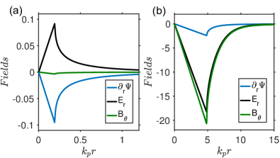
Figure 2: The radial electric field $E_{r}$, the radial gradient of the wakefield potential $\partial\psi/\partial r$ and azimuthal magnetic field $B_{\theta}$ as a function on radius $r$ at $\xi=0.5$: (a) $Q=0.01$ and (b) $Q=25$. Bubble boundaries are at $r\approx 0.19$ in (a) and $r\approx 5$ in (b).

V.2 Plasma bubble and secondary plasma waves.

Figure 3 shows characteristics of the plasma flow in the wake of pointlike bunch of ultrarelativistic electrons with $Q=25$ and $Q=100$. The scales of the panels suggest that the bubble dimensions are proportional to $Q^{1/2}$. The radius $R_{b}$ of the plasma bubble is slightly larger than half of the bubble length $L_{b}$; the bubble resembles a deformed sphere. Note that the bubble boundary has many kinks in its rear part where plasma streams inject electrons into the bubble (see panels (a) and (b) in Fig. 3).

The wakefield potential is positive inside the bubble and its maximum value is $\psi\propto R_{b}^{2}\propto Q$. The dashed white lines in Fig. 3 (c) and (d) border the areas where $\psi$ is large. The magnetic field is negative inside the bubble (see panels (e) and (f) in Fig. 3). It grows with the driver charge as $Q^{1/2}$.

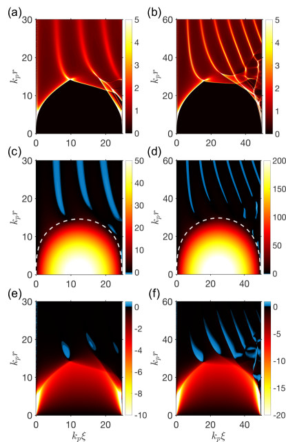
Figure 3: Plasma characterisics at large driver charge $Q=25$ (frist column) and $Q=100$ (second column): density $n_{e}$ (upper panels), wakefield potential $\psi$ ( middle panels), and magnetic field $B_{\theta}$ (lower panels). Red color on panels (e) and (f) denotes negative value of the magnetic field.

To verify the scaling laws, we have performed PIC simulations for a range of driver charges. Figure 4 (a) shows plasma bubble boundaries at large $Q$. The radius and length of the bubble are approximated at large $Q$ as $R_{b}\approx 2.8Q^{1/2}$ and $L_{b}\approx 4.9Q^{1/2}$.

It is noteworthy that the ratio $R_{b}/Q^{1/2}$ is nearly constant within the explored range of the driver charges as indicated by the blue curve in Fig. 4 (b). This ratio is 2.8 at small $Q$, reaches a minimum of $2.5$ at $Q\approx 1$ and then returns to the value $2.8$ at large $Q$. The length of the plasma bubble has a constant value stupakov_wake_2016 at small $Q$ and it is approximated as $L_{b}\approx 4.9Q^{1/2}$ at large $Q$. One can see in Figure 4 (a) exhibits some deviation of the bubble length from the $Q^{1/2}$-scaling already at $Q=5$.

Figure 3 also shows reveals oscillations of the plasma density $\delta n_{e}$ outside the bubble; these oscillations are correlated with the narrow stream of energetic particles expelled by the driver charge. Since the density of energetic (hot) electrons $n_{h}$ is small at large distances ($r\gg Q^{1/2}\gg 1$), the oscillations of cold plasma are weak and can be described in the linear approximation ($\psi<<1$, $\gamma\approx 1$, $\delta n_{e}=\delta n_{*}-\psi\ll 1$). Linearizing Eqs. (9), (15) and (20), we obtain:

$$\frac{\partial^{2}}{\partial\xi^{2}}\delta n_{e}+\delta n_{e}=-n_{h}.$$ (29)

The stream of energetic electrons is only weakly perturbed by the fields near the bubble. Consequently, we can use ballistic approximation to find $n_{h}$. Omitting the intermediate steps, we present the final approximate formula:

$$n_{h}=\frac{2Q^{2}}{r^{2}}F\bigg{(}\frac{Q\xi}{r}\bigg{)},\quad F\equiv\frac{1}{1+5(Q\xi/r)^{3/2}}.$$ (30)

Integrating Eq. (29) with initial conditions $\delta n_{e}|_{\xi=0+}=0$ and $(\partial\delta n_{e}/\partial\xi)|_{\xi=0+}=0$, we find that, at large $r$, its solution replicates the phase and amplitude of the plasma waves observed in the simulations. As predicted by Eq. (29), the plasma waves form vertical striations with a period $\Delta\xi=2\pi$. The number of striations scales with the driver charge as $L_{st}\propto L_{b}/2\pi\propto Q^{1/2}$. Therefore the flow pattern in the striation area lacks self-similarity.

At small distances from the bubble, the waves become nonlinear, and eventually brake. Merging with bubble boundary, the striations create kinks that destroy boundary smoothness.

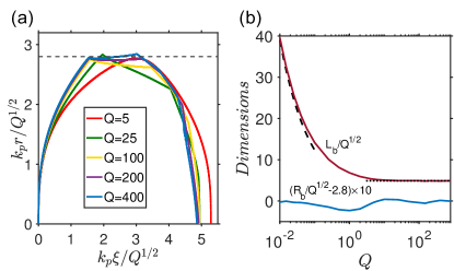
Figure 4: (a) Boundaries of plasma bubble at large $Q$ , and (b) dependence of the radius and length of the plasma bubble on $Q$ in the range $0.01\leq Q\leq 100$. Dashed line at the left corresponds to asymptote $L_{b}=3.8$ at small $Q$, while the right dashed line to asymptote $L_{b}=4.9Q^{1/2}$ at large $Q$.

One can show that small oscillations of the wakefield potential can be estimated as $\psi\approx-\delta n_{e}$, see Fig. 3 (c) and (d), while the magnetic field does not oscillate at all in the linear approximation [see Fig. 3 (e) and (f)].

VI Phenomenological models of plasma bubble at large $Q$

As already mentioned, the plasma bubble in the wake of the pointlike electron driver looks like a slightly deformed sphere when $Q$ is large. Yet, this small deformation brings new properties that are very different from those of spherical bubble Kostyukov_phenomenological_2004 . To demonstrate this difference, we develop a simple model that captures the essential features of the bubble observed in PIC simulations.

The simulations show that electromagnetic energy is mostly stored inside the bubble, where the electron density vanishes. To simplify the sheath structure, we assume that all fields vanish outside the bubble. Integration of Eq. (15) with $n_{*}=0$ gives the wakefield potential inside the bubble

$$\psi(\xi,r)=\psi(\xi,0)-\frac{1}{4}r^{2},$$ (31)

where $\psi(\xi,0)$ is an on-axis potential. It turns out that our simulation results suggest a very accurate approximation for the wakefield potential on the bubble axis. More specifically, $\psi(\xi,0)\cong\bar{\psi}(\xi)\equiv\frac{1}{4}\bar{r}_{b}(\xi)^{2}$ with $\bar{r}_{b}(\xi)$ defined by one-parameter equation

$$\frac{\bar{r}_{b}^{3}}{R_{b}^{3}}+{\bigg{(}1-\frac{\xi}{\xi_{c}}\bigg{)}^{2}}=1$$ (32)

where $\xi_{c}\equiv\frac{1}{2}L_{b}\approx(6Q)^{1/2}$ and $R_{b}\approx 3Q^{1/2}-0.2$. As seen in Fig. 5, Eq. (32) gives also a good approximation for $E_{z}(\xi,0)$. Function $\bar{r}_{b}(\xi)$ can be interpreted as a radius at which the wakefield potential $\psi(\xi,r)$ given by Eq. (31) formally vanishes. Such $\psi$-boundaries of the plasma bubble are smooth and denoted in Fig. 3 (c) and (d) by white dashed lines.

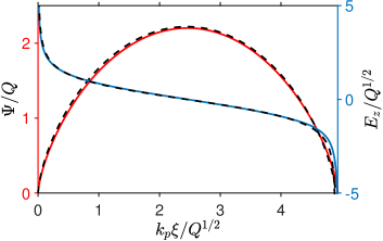
Figure 5: The wakefield potential $\psi$ (red) and the longitudinal electric field $E_{z}$ (blue) on the bubble axis obtained from PIC simulations at $Q=100$. Dashed lines correspond to fitting curves $\bar{\psi}(\xi)=\bar{r}_{b}^{2}(\xi)/4$ and $d\bar{\psi}(\xi)/d\xi$, where $\bar{r}_{b}(\xi)$ is defined by Eq. (32).

All fields inside the bubble can now be expressed through $\bar{r}_{b}(\xi)$:

$$\psi(\xi,r)=\bar{\psi}(\xi)-\frac{1}{4}r^{2},$$ (33)

$$\frac{\partial\psi}{\partial r}=-\frac{1}{2}r,\quad E_{z}=\frac{d\bar{\psi}(\xi)}{\partial\xi},\quad B_{\theta}=\frac{1}{2}\frac{\partial E_{z}}{\partial\xi}r,$$ (34)

where $r\leq\bar{r}_{b}(\xi)$, $0<\xi<2\xi_{c}$, and $\bar{\psi}(\xi)=\frac{1}{4}R_{b}^{2}[1-(1-\xi/\xi_{c})^{2}]^{2/3}$. Outside the bubble, these fields are set to zero. We see from these expressions, once again, that $\psi$ is proportional to $Q$ and $\partial_{r}\psi$, $E_{z}$, and $B_{\theta}$ are proportional to $Q^{1/2}$. These scalings do not hold in striations but the fields are relatively weak outside the bubble.

A spherical model of the bubble developed for a laser driver in Ref. Kostyukov_phenomenological_2004 suggests

$$\frac{\bar{r}_{b}^{2}}{R_{b}^{2}}+{\bigg{(}1-\frac{\xi}{R_{b}}\bigg{)}^{2}}=1,$$ (35)

where $R_{b}$ is the bubble radius and $0<\xi<2R_{b}$. In this case $\psi(\xi,r)=\frac{1}{4}[R_{b}^{2}-(R_{b}-\xi)^{2}-r^{2}]$ inside the bubble and $\psi(\xi,r)=0$ outside.

Equations (32) and (35) look very similar at first sight, especially if one takes into account that $\xi_{c}$ only slightly smaller than $R_{b}$. Despite this similarity, the fields are dramatically different at the bubble frontal parts. In the large charge model (32), we find that $\bar{r}_{b}\approx R_{b}(2\xi/\xi_{c})^{1/3}$ at $\xi\ll R_{b}$, and the magnetic field is very large: $B_{\theta}\approx-\frac{1}{9}r(R_{b}^{6}/\bar{r}_{b}^{4}\xi_{c}^{2})$. This field determines the radial electric field

$$E_{r}=-\partial\psi/\partial r+B_{\theta}\approx B_{\theta}$$ (36)

More accurate estimate shows that the radial electric field is negative up to $\xi=0.3\xi_{c}$. In contrast, $B_{\theta}\approx-\frac{1}{4}r$ in the spherical model, and the radial field is always positive $E_{r}=\frac{1}{4}r$.

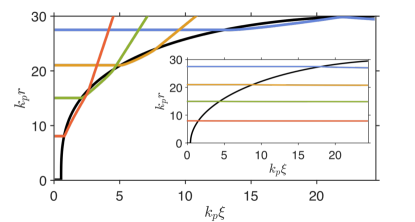
Figure 6: Trajectories of of test electrons initially placed at rest at different distances from the bubble axis. Electrons are repelled by the bubble in the large charge model (32) while the same electrons penetrate into the spherical bubble (35) (inset). In both models $R_{b}\approx 30$.

As a result, cold electrons experience strong repulsion at the frontal part of the bubble in the large charge model, while the same electrons are pulled inward in the spherical bubble case (see Fig. 6).

One can get a better understanding of the structural difference between these bubbles by examining a part of energy (11) associated with the wakefield potential:

$$U_{pot}=2\pi\int_{0}^{\infty}rdr\frac{[\nabla\psi(\xi,r)]^{2}}{2}$$ (37)

where $(\nabla\psi)^{2}=E_{z}^{2}+(\partial\psi/\partial r)^{2}$. At $\xi<<R_{b}$, the contribution from the radial gradient of the wakefield potential can be neglected. Hence, $(\nabla\psi)^{2}\approx E_{z}^{2}$ and $U_{pot}\approx\frac{1}{2}\pi E_{z}^{2}r_{b}^{2}$. Since $E_{z}^{2}\approx R_{b}^{2}/4$ and $r_{b}^{2}\approx 2R_{b}\xi$, the initial potential energy in the spherical model (35) vanishes: $U_{pot}|_{\xi=+0}=0$. In contrast, $E_{z}^{2}\propto 1/r_{b}^{2}$ and the initial potential energy is finite in the large charge model (32): $U_{pot}\approx 21Q^{2}$. This potential energy determines subsequent evolution of the plasma bubble: change in $E_{z}$ creates a displacement current $\partial E_{z}/\partial\xi$ that generates strong magnetic field $B_{\theta}$ which, in turn, induces the radial electric field $E_{r}$ (36).

Analysis of the bubble energy reveals additional interesting aspects of the bubble behind the large charge driver. Figure 7 shows that the total energy of the system in the quasistatic PIC simulations (plotted by black line) remains constant in agreement with Eq. (11). The potential energy in the $E_{z}$-component of the electric field approximately doubles during very short ‘time’ $\xi<<1$ via energy transfer from macroparticles. After that, $E_{z}$ field energy slowly, while the energy attributable to the radial gradient of the wakefield potential increases till $\xi<\xi_{c}$. Unexpectedly, variation of the total potential energy (plotted by red line) with ‘time’ $\xi$ is relatively small (within $17\%$). Note that the fields are nearly zero outside the bubble and $E_{z}=\frac{1}{2}\bar{r}_{b}(d\bar{r}_{b}/d\xi)$ and $\partial\psi/\partial r=-\frac{1}{2}r$ inside the bubble. Given that variation of the potential energy is relatively small, one can now write the energy balance equation as

$$\frac{1}{8}\pi\bar{r}_{b}^{4}\Big{(}\frac{d\bar{r}_{b}}{d\xi}\Big{)}^{2}+\frac{1}{16}\pi\bar{r}_{b}^{4}=\frac{1}{16}\pi R_{b}^{4}$$ (38)

where $\frac{1}{16}\pi R_{b}^{e}$ is the potential energy at $\xi=\xi_{c}$. A straighforward solution of this equation shows that the bubble is a deformed sphere with half length $\xi_{c}\approx 0.85R_{b}$ that is slightly longer than the length obtained from PIC simulations. Furthermore, differentiation of Eq. (38) with respect to $\xi$ gives

$$\bar{r}_{b}\frac{d^{2}\bar{r}_{b}}{d\xi^{2}}+2\Big{(}\frac{d\bar{r}_{b}}{d\xi}\Big{)}^{2}+1=0.$$ (39)

The same equation follows from the model developed by Lu et al. Lu_theory_2006 . Therefore, despite the fact that the boundary of the plasma bubble created by the pointlike driver is composed of many electron trajectories, the Lu model is supported by the approximate conservation of the potential energy.

Figure 7: Change of the energy with ‘time’ $\xi$ for (a) $Q=25$ and (b) $Q=100$ observed in PIC simulations: the kinetic energy of macroparticles in the region $r<2R_{b}$(brown), the potential energy stored in $E_{z}$ (green), potential energy stored in $\partial_{r}\psi$ (blue), total potential energy (red), and total energy of the system normalized by $2Q^{2}$ (black).

We conclude this section by noting that integral (11) logarithmically diverges at the lower limit at $\xi=0+$, because $\langle\gamma-1\rangle|_{\xi=0+}\approx 1/r^{2}$ at small $r$. For this reason, the total energy of the system increases with increase of simulation resolution. But this increase does not influence the plasma electron flow and does not change the ‘time’-evolution of the potential energy at sufficiently small size of the radial cell: $\Delta r\ll 1$.

VII Summary

We have advanced the nonlinear wakefield theory in quasistatic approximation and developed a novel PIC code in which all fields are determined from static equations. More specifically, the wakefield potential is found from the Poisson equation and the magnetic field is found from the Helmholtz equation. The source terms in these equations depend only on radial positions and momenta of macroparticles. This approach can be straightforwardly generalized to the case of nonaxisymmetric plasma flows, see Appendix C.

We have characterized the plasma flow in the wake of a pointlike bunch of ultrarelativistic electrons. The radius and the length of the plasma bubble are found for varying values of the bunch charge. We show that the normalized bubble radius $R_{b}/Q^{1/2}$ is approximately equal to $2.8$ for small and large values of $Q$, and only slightly deviates from $2.8$ at $Q\sim 1$. The normalized length of the bubble has a constant value 3.8 for $Q\ll 1$, and grows as $L_{b}\approx 4.9Q^{1/2}$ at $Q\gg 1$.

Our phenomenological models for large $Q$ explain how small deviation of the bubble from the spherical shape can dramatically change the bubble properties. by comparing a large charge model (32) with spherical one (35). These models reveal the governing role of the potential energy (37) on the bubble structure that reflects transformation from the energy stored in the field $E_{z}$ to the energy stored in the field $\partial_{r}\psi$, and vice versa.

Our simulations and analytical theory reveal plasma waves excited by energetic particles at large distances from the bubble. The amplitude of these waves becomes large near the bubble giving rise to wavebreaking. When present at the bubble boundary, striations of plasma waves create kinks destroying boundary smoothness.

This research was supported by DOE grants DE-SC0007889 and DE-SC0010622, and by an AFOSR grant FA9550-14-1-0045. B. Breizman was supported by the U.S. Department of Energy Contract No. DEFG02-04ER54742.

Appendix A Vlasov’s equation in the cylindrically symmetric form.

It is convenient to write Eq. (2) in the form:

$$\frac{\partial}{\partial t}{f_{e}}+\frac{\partial}{\partial{\bf{R}}}\cdot\bigg{(}\frac{\partial H}{\partial{\bf{P}}}f_{e}\bigg{)}-\frac{\partial}{\partial{\bf{P}}}\cdot\bigg{(}\frac{\partial H}{\partial{\bf{R}}}f_{e}\bigg{)}=0,$$ (40)

We replace $\partial/\partial t\rightarrow\partial/\partial\xi$ and $\partial/\partial z\rightarrow-\partial/\partial\xi$, substitute the electron distribution function $f_{e}$ using Eq. (6) and then integrate Eq. (40) over longitudinal and azimuthal momenta. Taking into account that the function $\delta(H-P_{z}-1)$ integrated over $P_{z}$ produces the factor $1/(1-v_{z})=\gamma/(1+\psi)$, we obtain:

$$\frac{\partial}{\partial\xi}{rf_{*}}+\frac{\partial}{\partial{r}}\bigg{(}\frac{\partial H}{\partial{p_{r}}}\frac{\gamma rf_{*}}{1+\psi}\bigg{)}-\frac{\partial}{\partial{p_{r}}}\bigg{(}\frac{\partial H}{\partial{r}}\frac{\gamma rf_{*}}{1+\psi}\bigg{)}=0,\,\,\,\,$$ (41)

Noting that Hamiltonian $H_{*}$ defined by Eq. (8) satisfies the relations:

$$\frac{\partial H_{*}}{\partial{p_{r}}}=\frac{\partial H}{\partial{p_{r}}}\frac{\gamma}{1+\psi},\quad\frac{\partial H_{*}}{\partial{r}}=\frac{\partial H}{\partial{r}}\frac{\gamma}{1+\psi},$$ (42)

one can straightforwardly transform Eq. (41) to Eq. (7).

Appendix B Conservation of energy of macroparticles.

Energy conservation in differential form is given by

$$\frac{\partial}{\partial t}\bigg{[}W+\frac{1}{2}(E^{2}+B^{2})\bigg{]}+\nabla\cdot({\bf{J}}+{\bf{E}}\times{\bf{B}})=0,$$ (43)

where $W=\int d^{3}{\bf{p}}f_{e}(\gamma-1)$ is the density of electron kinetic energy and ${\bf{J}}$ is its flux. Replacing $t$ and $-z$ by $\xi$ and performing integration in the transverse plane, we obtain

$$\frac{\partial}{\partial\xi}\int d^{2}{\bf{r}}_{\perp}\bigg{[}W-J_{z}+\frac{E^{2}+B^{2}}{2}-[{\bf{E}}\times{\bf{B}}]_{z}\bigg{]}=0.$$ (44)

One can directly check that $W-J_{z}=n_{*}\langle\gamma-1\rangle$ and $\frac{1}{2}(E^{2}+B^{2})-[{\bf{E}}\times{\bf{B}}]_{z}=\frac{1}{2}[E_{z}^{2}+(\partial_{r}\psi)^{2}]$ in the cylindrically symmetric case, i.e., Eq. (11) follows from Eq. (44).

Appendix C Nonaxisymmetric plasma flows

In this section we present a condensed derivation of the basic equations under quasistatic approximation for nonaxisymmetric plasma flows. The current density of the driving electron beam is given now by

$$j_{dr}=4\pi Q\delta(x)\delta(y)\delta(t-z).$$ (45)

Assuming that the distribution function $f_{e}$ and electromagnetic fields depend on t and z only through a combination $\xi=t-z$, we find that $H-P_{z}-1=0$. The distribution function of electrons can be expressed in the form

$$f_{e}(t,{\bf{R}},{\bf{P}})=f_{*}(\xi,{\bf{r}},{\bf{P}}_{\perp})\delta(H-P_{z}-1),$$ (46)

where $f_{*}$ represents now a distribution function of macroparticles performing two dimensional motion in the $(x,y)$-plane and ${\bf{r}}\equiv(x,y)$. Substituting Eq. (46) into (3), we find that $f_{*}$ satisfies the Vlasov equation:

$$\frac{\partial{f}_{*}}{\partial\xi}+\frac{\partial H_{*}}{\partial{\bf{P}}_{\perp}}\cdot\frac{\partial f_{*}}{\partial{\bf{r}}}-\frac{\partial H_{*}}{\partial{\bf{r}}}\cdot\frac{\partial f_{*}}{\partial{\bf{P}}_{\perp}}=0,$$ (47)

where

$$H_{*}=\frac{1+({\bf{P}}_{\perp}+{\bf{A}}_{\perp})^{2}+(1+\psi)^{2}}{2(1+\psi)}-\psi-A_{z}$$ (48)

is the Hamiltonian for the two-dimensional motion in the $(x,y)$-plane and $\psi=\phi-A_{z}$ is the wakefield potential. The trajectory of an individual particle in the phase space $({\bf{r}},{\bf{P}}_{\perp})$ is determined by equations of motion

$$\frac{d{\bf{P}}_{\perp}}{dt}=-\frac{\partial H}{\partial{\bf{r}}},\quad\frac{d{\bf{r}}}{dt}=\frac{\partial H}{\partial{\bf{P}}_{\perp}}.$$ (49)

By replacing ${\bf{P}}_{\perp}={\bf{p}}_{\perp}-{\bf{A}}_{\perp}$, these equations can be written in the form

$$\frac{d}{d\xi}{\bf{p}}_{\perp}=\frac{\gamma\nabla_{\perp}\psi}{1+\psi}+[{\bf{e}}_{z}\times{\bf{V}}]B_{z}+[{\bf{e}}_{z}\times{\bf{B}}_{\perp}],$$ (50)

$$\frac{d}{d\xi}{\bf{r}}_{\perp}\equiv{\bf{V}}_{\perp}=\frac{1}{1+\psi}{\bf{p}}_{\perp}$$ (51)

where $\gamma=[{1+{\bf{p}}_{\perp}^{2}+(1+\psi)^{2}}]/{2(1+\psi)}$ is the relativistic factor, and ${\bf{V}}\equiv{\bf{p}}_{\perp}/({1+\psi})$ is the particle ‘velocity’ in $(x,y)$-plane. Integration of Eq. (47) over $P_{x}$ and $P_{y}$ gives the continuity equation:

$$\frac{\partial}{\partial\xi}n_{*}=-\nabla_{\perp}\cdot(n_{*}\langle{\bf{V}}\rangle),$$ (52)

where $n_{*}=\int dP_{x}dP_{y}f_{*}$ is the density of macroparticles and the brackets denote averaging over transverse momentum $\langle{\bf{V}}\rangle={{n}}_{*}^{-1}\int dP_{x}dP_{y}f_{*}{\bf{V}}$.

We also note that the density and the current density of plasma electrons can be expressed through the distribution function $f_{*}$ as:

$$n_{e}=\frac{n_{*}\langle\gamma\rangle}{1+\psi},\quad{\bf{j}}_{\perp}=n_{*}\langle{\bf{V}}\rangle,\quad j_{z}=\frac{n_{*}\langle p_{z}\rangle}{1+\psi},$$ (53)

where $\langle p_{z}\rangle=\langle\gamma\rangle-\psi-1=[1+\langle{\bf{p}}_{\perp}^{2}\rangle-(1+\psi)^{2}]/(2(1+\psi)$. Besides, $n_{e}-j_{z}=n_{*}$.

Using the similar transformations as in Section II, we obtain the following equations

$$\Delta_{\perp}\psi=n_{*}-1,$$ (54)

$$\Delta_{\perp}E_{z}=-\nabla_{\perp}\cdot{\bf{j}}_{\perp},$$ (55)

$$\Delta_{\perp}B_{z}={\bf{e}}_{z}\cdot[\nabla_{\perp}\times{\bf{j}}_{\perp}],$$ (56)

$$\Delta_{\perp}{\bf{B}}_{\perp}=-[{\bf{e}}_{z}\times\nabla_{\perp}j_{z}]-\bigg{[}{\bf{e}}_{z}\times\frac{\partial}{\partial\xi}{\bf{j}}_{\perp}\bigg{]}.$$ (57)

The solutions of Poisson Eqs. (54) - (56) must vanish at $r\rightarrow\infty$. To obtain a closed form of Eq. (57), we multiply the Vlasov Eq. (47) by the ’velocity’ ${\bf{V}}_{\perp}=\partial H/\partial{\bf{P}}_{\perp}$ and integrate it over momentum. After straightforward calculations we find

$$\frac{\partial}{\partial\xi}{\bf{j}}_{\perp}=n_{*}\langle{\bf{a}}\rangle-\frac{\partial}{\partial x}n_{*}\langle V_{x}{\bf{V}}_{\perp}\rangle-\frac{\partial}{\partial y}n_{*}\langle V_{y}{\bf{V}}_{\perp}\rangle.$$ (58)

where ${\bf{a}}\equiv{d^{2}{\bf{r}}_{\perp}}/{d\xi^{2}}$ is the particle ’acceleration’:

$${\bf{a}}=\frac{[{\bf{e}}_{z}\times{\bf{B}}_{\perp}]}{1+\psi}+\frac{[{\bf{e}}_{z}\times{\bf{V}}_{\perp}]B_{z}}{(1+\psi)}+\tilde{\bf{a}},$$ (59)

$$\tilde{\bf{a}}=\frac{\gamma\nabla_{\perp}\psi}{(1+\psi)^{2}}-\frac{{\bf{V}}}{1+\psi}\bigg{(}E_{z}+{\bf{V}}\cdot\nabla_{\perp}\psi\bigg{)}.$$ (60)

Substituting ${\partial{\bf{j}}_{\perp}}/{\partial\xi}$ from Eq. (58) to Eq. (57) we obtain Helmholtz equation describing the transverse magnetic field:

$$\Delta_{\perp}{\bf{B}}_{\perp}=\frac{n_{*}}{1+\psi}{\bf{B}}_{\perp}-[{\bf{e}}_{z}\times{\bf{S}}]$$ (61)

with the source

$${\bf{S}}=\frac{[{\bf{e}}_{z}\times n_{*}\langle{\bf{V}}\rangle]B_{z}}{(1+\psi)}+n_{*}\langle\tilde{\bf{a}}\rangle-$$

$$\frac{\partial}{\partial x}n_{*}\langle V_{x}{\bf{V}}_{\perp}\rangle-\frac{\partial}{\partial y}n_{*}\langle V_{y}{\bf{V}}_{\perp}\rangle+\nabla_{\perp}j_{z}.$$ (62)

The solutions of Eq. (61) must vanish at $r\rightarrow\infty$. Thus, in quasi-static approximation all fields are determined from static Eqs. (54) - (56) and (61) by positions and momenta of macroparticles in the plane $(x,y)$ at given ‘time’ $\xi$. The source terms in these equations do not have ‘time’ derivatives of the fields or currents.

When these equations are incorporated in the PIC code, it is convenient to replace an averaging over transverse components of the canonical momentum by the averaging over corresponding components of the kinetic momentum. Indeed, since ${\bf{P}}_{\perp}={\bf{p}}_{\perp}-{\bf{A}}_{\perp}$ and averaging is performed at given point ${\bf{r}}$, we obtain

$$\frac{1}{n_{*}}\int dP_{x}dP_{y}f_{*}(\xi,{\bf{r}},{\bf{P}}_{\perp}){\bf{V}}=$$

$$\frac{1}{n_{*}}\int dp_{x}dp_{y}f_{*}(\xi,{\bf{r}},{\bf{p}}_{\perp}-{\bf{A}}_{\perp}){\bf{V}}.$$ (63)

References

- (1) P. Chen, J. M. Dawson, R. W. Huff, T. Katsouleas, ”Acceleration of Electrons by the Interaction of a Bunched Electron Beam with a Plasma,” Phys. Rev. Lett., vol. 54, 693 (1985).
- (2) T. Tajima, J. M. Dawson, ”Laser Electron Accelerator,” Phys. Rev. Lett, vol. 43, 267 (1979).
- (3) I. Blumenfeld, C. E. Clayton, F.-J. Decker, M. J. Hogan, C. Huang, R. Ischebeck, R. Iverson, C. Joshi, T. Katsouleas, N. Kirby, W. Lu, K. A. Marsh, W. B. Mori, P. Muggli, E. Oz, R. H. Siemann, D. Walz, M. Zhou, ”Energy doubling of 42 GeV electrons in a metre-scale plasma wakefield accelerator,” Nature, vol. 445, 741–744 (2007).
- (4) J. B. Rosenzweig, B. Breizman, T. Katsouleas, J. J. Su, ”Acceleration and focusing of electrons in two-dimensional nonlinear plasma wake fields,” Phys. Rev. A, vol. 44, R6189 (1991).
- (5) R. A. Fonseca, L. O. Silva, F. S. Tsung, V. K. Decyk, W. Lu, C. Ren, W. B. Mori, S. Deng, S. Lee, T. Katsouleas, J. C. Adam, ”OSIRIS: A Three-Dimensional Fully Relativistic Particle in Cell Code for Modeling Plasma Based Accelerators,” in: P.M.A. Sloot, C.J.K. Tan, J.J. Dongarra, A.G. Hoekstra (Eds.), Computational Science - ICCS 2002, Part III, Lecture Notes in Computational Science, vol. 2331, Springer, p. 342 (2002)
- (6) A. Pukhov, ”Three-dimensional electromagnetic relativistic particle-in-cell code VLPL (Virtual Laser Plasma Lab),” J. Plasma Physics vol. 61, 425-433 (1999).
- (7) C. Nieter, J. R. Cary, ”VORPAL: a versatile plasma simulation code,” J. Comput. Phys., vol. 196, 448 (2004).
- (8) P. Sprangle, E. Esarey, and A. Ting, ”Nonlinear Theory of Intense Laser-Plasma Interactions,” Phys. Rev. Lett. vol. 64, 2011 (1990).
- (9) P. Mora, T. M. Antonsen Jr., ”Kinetic modeling of intense, short laser pulses propagating in tenuous plasmas,” Phys. Plasmas vol. 4, 217 (1997).
- (10) K. V. Lotov, ”Fine wakefield structure in the blowout regime of plasma wakefield accelerators,” Phys. Rev. ST Accel. Beams, vol. 6, 061301 (2003).
- (11) C. Huang, V.K. Decyk, C. Ren, M. Zhou, W. Lu, W.B. Mori, J.H. Cooley, T.M. Antonsen Jr., T. Katsouleas, ”QUICKPIC: A highly efficient particle-in-cell code for modeling wakefield acceleration in plasmas,” J. Comp. Phys., vol. 217, 658-679 (2006).
- (12) I. Kostyukov, A. Pukhov, S. Kiselev, ”Phenomenological theory of laser-plasma interaction in “bubble” regime,” Phys. Plasmas vol. 11, 5256 (2004).
- (13) W. Lu, C. Huang, M. Zhou, M. Tzoufras, F. S. Tsung, W. B. Mori, T. Katsouleas, ”A nonlinear theory for multidimensional relativistic plasma wave wakefields,” Phys. Plasmas vol. 13, 056709 (2006).
- (14) S. A. Yi, V. Khudik, C. Siemon, G. Shvets, ”Analytic model of electromagnetic fields around a plasma bubble in the blow-out regime,” Phys. Plasmas vol. 20, 013108 (2013).
- (15) N. Barov, J. B. Rosenzweig, M. C. Thompson, R. B. Yoder, ”Energy loss of a high-charge bunched electron beam in plasma: Analysis,” Phys.Rev.ST Accel.Beams, vol. 7, 061301 (2004).
- (16) G. Stupakov, B. Breizman, V. Khudik, G. Shvets, ”Wake excited in plasma by an ultrarelativistic pointlike bunch,” Phys.Rev.ST Accel.Beams, vol. 19, 101302 (2016).
- (17) J. B. Rosenzweig, N. Barov, M. C. Thompson, R. B. Yoder, ”Energy loss of a high-charge bunched electron beam in plasma: Simulations, scaling, and accelerating wakefields,” Phys.Rev.ST Accel.Beams, vol. 7, 061302 (2004).
- (18) Charles K. Birdsall, A. Bruce Langdon, ”Plasma physics via computer simulation. CRC press,” (Adam Hilger, Bristol, 1991)
- (19) R. Keinigs, M. E. Jones, , ”Two-dimensional dynamics of the plasma wakefield accelerator,” Phys. Fluids vol. 30, 252 (1987).
- (20) R. L. Burden, J. D. Faires, A. M. Burden, ”Numerical Analysis,” (Cengage Learning, 2015)