Spin Ice Thin Films: Large-N Theory and Monte Carlo Simulations

Abstract

We explore the physics of highly frustrated magnets in confined geometries, focusing on the Coulomb phase of pyrochlore spin ices. As a specific example, we investigate thin films of nearest-neighbor spin ice, using a combination of analytic large-$N$ techniques and Monte Carlo simulations. In the simplest film geometry, with surfaces perpendicular to the $[001]$ crystallographic direction, we observe pinch points in the spin-spin correlations characteristic of a two-dimensional Coulomb phase. We then consider the consequences of crystal symmetry breaking on the surfaces of the film through the inclusion of orphan bonds. We find that when these bonds are ferromagnetic, the Coulomb phase is destroyed by the presence of fluctuating surface magnetic charges, leading to a classical $Z_{2}$ spin liquid. Building on this understanding, we discuss other film geometries with surfaces perpendicular to the $[110]$ or the $[111]$ direction. We generically predict the appearance of surface magnetic charges and discuss their implications for the physics of such films, including the possibility of an unusual $Z_{3}$ classical spin liquid. Finally, we comment on open questions and promising avenues for future research.

I Introduction

The emergence of gauge structures in strongly correlated systems has proven to be an essential thread in the fabric of modern condensed matter physics Kogut (1979); Nagaosa (1999); Wen (2004); Lee et al. (2006). In the prototypical example of a gauge theory – electromagnetism – boundary conditions can play a key role in the physics Jackson (2007). Indeed, realizations of gauge theories in systems with confined geometries can lead to rich and varied phenomena as, for example, in the Casimir effect Milton (2001); Bordag et al. (2001). In the same spirit, questions pertaining to surface effects in emergent gauge theories of strongly correlated systems, have only recently begun to be addressed Wang and Senthil (2016). A paradigmatic example where such an emergent $U(1)$ gauge theory arises is in spin ice materials Harris et al. (1997); Ramirez et al. (1999), a class of highly frustrated three-dimensional magnets. Given the level of maturity of research on spin ice Bramwell et al. (2004); Gingras (2011), with many theoretical successes and several well-understood experimental examples, it is a natural system to explore the effects of confined geometries in emergent gauge theories.

In the prototypical spin ice materials Dy₂Ti₂O₇ and Ho₂Ti₂O₇, the magnetic moments reside on the sites of a pyrochlore lattice, which is formed of corner-sharing tetrahedra, as shown in Fig. 1. At low temperatures, these magnetic moments are forced by the crystalline electric field Rau and Gingras (2015) to point either in or out of any given tetrahedron. The strongly frustrated interactions between the magnetic moments then give rise to a local “2-in/2-out” constraint on every tetrahedron in the ground state, a close of analogue of the arrangement of protons in common water ice Bramwell et al. (2004); Gingras (2011). This constraint can be rewritten in a form similar to Gauss’ law in electromagnetism Henley (2005), giving rise to an emergent Coulomb phase Henley (2010); Castelnovo et al. (2012) in these materials. This phase is characterized by algebraic spin correlations with fractionalized excitations taking the form of emergent magnetic monopoles Castelnovo et al. (2008, 2012). Furthermore, quantum models of spin ice materials have been suggested as promising platforms to realize a related quantum spin liquid phase Gingras and McClarty (2014).

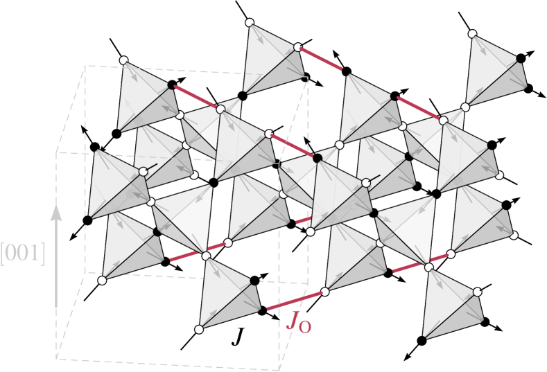
Figure 1: Spin ice film of thickness $L=1$. The magnetic ions form a pyrochlore lattice, composed of corner-sharing tetrahedra. Cleaving the surfaces perpendicular to the $[001]$ direction exposes orphan bonds on the top and bottom surfaces, not belonging to any complete tetrahedron (shown in red). These orphan bonds have an exchange coupling $J_{\rm O}$ distinct from that of the other bonds, $J$

Research on spin ice materials has so far mainly focused on bulk properties Gingras (2011). In water ice, some interesting physics has been found by looking at the effects of confined geometries. For example, by squeezing water between two sheets of graphene Algara-Siller et al. (2015), one finds that the water molecules form a square lattice, reminiscent of the six-vertex model. The investigation of spin ice films in such confined geometries – thin films, in particular – is now developing Bovo et al. (2014); Petrenko (2014); Leusink et al. (2014). Very recently, the first films of Dy₂Ti₂O₇ Bovo et al. (2014) and Ho₂Ti₂O₇ Leusink et al. (2014) were grown, with Ref. [Bovo et al., 2014] reporting a vanishing residual entropy at low temperature, in strong contrast with bulk physics . The theoretical work to date has tackled a variety of issues; for example, Refs. [She et al., 2017,Sasaki et al., 2014] considered heterostructures involving spin ice materials, while Jaubert et al. (2017) investigated the dipolar spin ice model in a thin film geometry using Monte Carlo methods. However, to the best of our knowledge, there currently is no theoretical understanding of even the simplest minimal model, that of nearest-neighbor spin ice films.

In this paper, we explore the physics of nearest-neighbor spin ice films, considering the fate of the three-dimensional Coulomb phase as well as the effects of different surface terminations. We take a two-pronged approach: we use the analytical large-$N$ method, which has been successful in applications to bulk spin ice Isakov et al. (2004) and films of ferromagnets Dantchev et al. (2014), and validate its predictions for nearest-neighbor spin ice films using Monte Carlo simulations. We focus our investigation on the simplest highly symmetric film geometry, with surfaces perpendicular to the crystallographic $[001]$ direction. We find that: (i) The characteristic pinch points found in the spin-spin correlations Henley (2005, 2010) of bulk spin ice remain intact for momenta parallel to the surfaces, a signature of a two-dimensional Coulomb phase (a classical $U(1)$ spin liquid). (ii) The direct space spin-spin correlations oscillate as a function of depth in the sample, with an amplitude that increases with decreasing temperature. (iii) By including orphan bonds to capture some of the crystal symmetry breaking of the film surfaces, we find that the Coulomb phase and its associated pinch points disappear when the exchange on the orphan bonds is ferromagnetic, yielding a classical $Z_{2}$ spin liquid Rehn et al. (2017). These results are summarized in the phase diagram shown in Fig. 2. Finally, building on this understanding, we extend these results to discuss the surface states of films with cleaved surfaces perpendicular to the $[110]$ or $[111]$ direction. From general considerations, we predict the appearance of surface magnetic charges in the ground state, akin to the monopoles realized as excitations in bulk spin ice. We discuss some implications of these surface charges, offering guidance for future studies on spin ice films with such geometries.

The rest of the paper is organized as follows: in Sec. II, we detail our model and then, in Sec. III, develop the large-$N$ formalism used to investigate spin ice films. In Sec. IV, we apply the large-$N$ method to films with surfaces perpendicular to the $[001]$ direction, and compare these results to those obtained from Monte Carlo simulations. In Sec. V, we discuss the topological order of the classical $U(1)$ and $Z_{2}$ spin liquids found in these films. Sec. VI briefly addresses other cleaving geometries, while Sec. VII offers concluding remarks and comments on possible avenues for future research. In Apps. A and B, we provide details of the large-$N$ theory for bulk spin ice and $[001]$ films. In App. C, we discuss the numerical solution of the large-$N$ saddle point equations. Finally, in App. D, we provide details of the Monte Carlo algorithm used to simulate Ising ($N=1$) spin ice films.

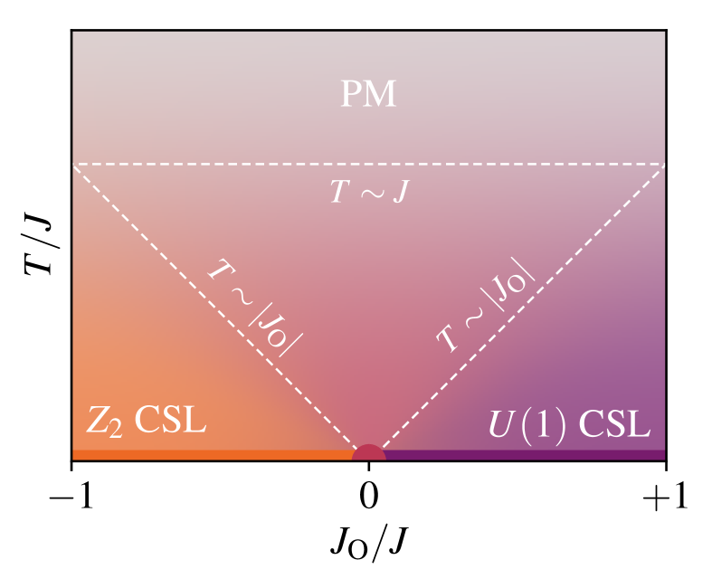
Figure 2: Phase diagram of $[001]$ thin films of spin ice as a function of temperature and orphan bond coupling $J_{\rm O}/J$ [see Eq. (2)]. The state at low temperature is either a classical $U(1)$ spin liquid ($J_{\rm O}/J>0)$ or a classical $Z_{2}$ spin liquid ($J_{\rm O}/J<0$). Two broad crossovers at $T\sim J$ and $T\sim|J_{\rm O}|$ (dashed lines) separate these phases from the high-temperature paramagnet (PM). For thick films, there is an additional crossover (not shown) where three-dimensional bulk spin ice behavior is recovered for $T\gtrsim J/\log L$.

II Model

II.1 Nearest-neighbor spin ice model

To set the stage, we first review the essential features of the nearest-neighbor ( nearest neighbor (NN)) spin ice model and then, in Sec. II.2, we minimally extend it to the context of films.

Recall that in classical spin ice Rau and Gingras (2015), the magnetic moments are represented by pseudospins $\bm{S}_{i}=\sigma_{i}\bm{\hat{z}}_{i}$ living on pyrochlore lattice sites labeled by $i$, where $\sigma_{i}=\pm 1$ is a classical Ising variable and $\hat{\bm{z}}_{i}$ are unit vectors along the local quantization axes (see App. A). In this work, we consider the simplest spin ice model, which only takes into account NN Ising exchange interactions. In the bulk this is the celebrated pyrochlore Ising antiferromagnet model Anderson (1956)

$$H=J\sum_{\langle ij\rangle}\sigma_{i}\sigma_{j},$$ (1)

where $J>0$, and the sum runs over NN bonds of the pyrochlore lattice. This Hamiltonian has a degenerate ground state manifold where every tetrahedron respects the local ice rules, i.e. the sum of Ising spins on every tetrahedron is zero. This realizes a classical $U(1)$ spin liquid, with an extensive ground-state degeneracy that remains down to zero temperature, thus giving a nonzero residual entropy.

The structure of the ground-state manifold can be formulated in terms of a coarse-grained effective “magnetic” field $\bm{B}(\bm{r})$ defined on each tetrahedron as $\bm{B}(\bm{r})\equiv(-1)^{\bm{r}}\sum_{i\in\bm{r}}\sigma_{i}\bm{\hat{z}}_{i}$, where the sign, $(-1)^{\bm{r}}$, depends on the sublattice of the tetrahedron in the dual diamond lattice (see Ref. [Henley, 2010] for a review). In terms of $\bm{B}$, the ice-rule constraint amounts to a divergence-free condition, $\bm{\nabla}\cdot\bm{B}=0$. Excitations above the spin ice ground-state manifold appear as pointlike sources or sinks of the field $\bm{B}$, behaving effectively as deconfined magnetic monopoles Castelnovo et al. (2008). At low temperatures, an analogue of classical magnetostatics thus emerges and induces a cooperative paramagnetic state dubbed a “Coulomb phase” Henley (2010). The divergence-free constraint also implies dipolar spin-spin correlations which manifest themselves as sharp “pinch points” in reciprocal space Henley (2005, 2010).

Even though it appears greatly simplified compared to dipolar spin-ice ( dipolar spin ice (DSI)) materials den Hertog and Gingras (2000) such as Dy₂Ti₂O₇ and Ho₂Ti₂O₇, the NN model captures much of the essential physics of the Coulomb phase shared with more realistic DSI models Castelnovo et al. (2008); den Hertog and Gingras (2000); Isakov et al. (2005); Gingras and den Hertog (2001). Although they are the best examples, dipolar interactions are not the only route to realizing spin ice. Rare-earth magnets where super-exchange is dominant could potentially host more faithful realizations of NN spin-ice [Eq. (1)] due to the short-range nature of the exchange physics. For example, the Pr₂M₂O₇ family Zhou et al. (2008); Kimura et al. (2013); Sibille et al. (2016), recently discussed as quantum spin-ice Gingras and McClarty (2014) candidates, are expected to have NN Ising exchange that is significantly larger than the magnetostatic dipolar interactions Onoda and Tanaka (2010, 2011).

II.2 Film geometries and boundary conditions

In order to model NN spin ice films, one must first define the boundary conditions, such as choosing a cleaving plane along which to cut the pyrochlore lattice, exposing free surfaces to a putative vacuum. For simplicity, we consider a free standing film and ignore complications arising from the presence of a substrate Bovo et al. (2014); Leusink et al. (2014). Three highly symmetric choices are planes normal to the $[001]$, $[110]$ and $[111]$ cubic crystallographic directions. We note that $[110]$ films of Dy₂Ti₂O₇ have been grown by Bovo et al. (2014), while films of Ho₂Ti₂O₇ for all three geometries have been grown by Leusink et al. (2014). In Sec. IV, we investigate the $[001]$ geometry in detail using the large-$N$ formalism and Monte Carlo simulations. Apart from being the simplest film geometry, it allows a direct comparison with the investigation of DSI films recently reported in Ref. [Jaubert et al., 2017]. We briefly explore other surface terminations, namely $[110]$ and $[111]$, in Sec. VI.

Exposing surfaces perpendicular to the $[001]$ direction amounts to cutting two spins for each surface tetrahedron, as shown in Fig. 1. The resulting slab is comprised of stacked planes, or layers, on which the spins form chains oriented in the $[110]$ or $[1\bar{1}0]$ directions, alternatively, as shown in Fig. 3. For simplicity, we consider thicknesses corresponding to an integer number $L$ of conventional cubic unit cells, comprising $4L$ spin layers (which we label by $l$) where the top chains are along $[1\bar{1}0]$ and the bottom chains run along $[110]$. The primitive unit cell of the film thus comprises $4L$ layers and $8L$ spins (see App. B). The associated conventional unit cells for film thicknesses $L=1,3,5$ are shown in Fig. 3.

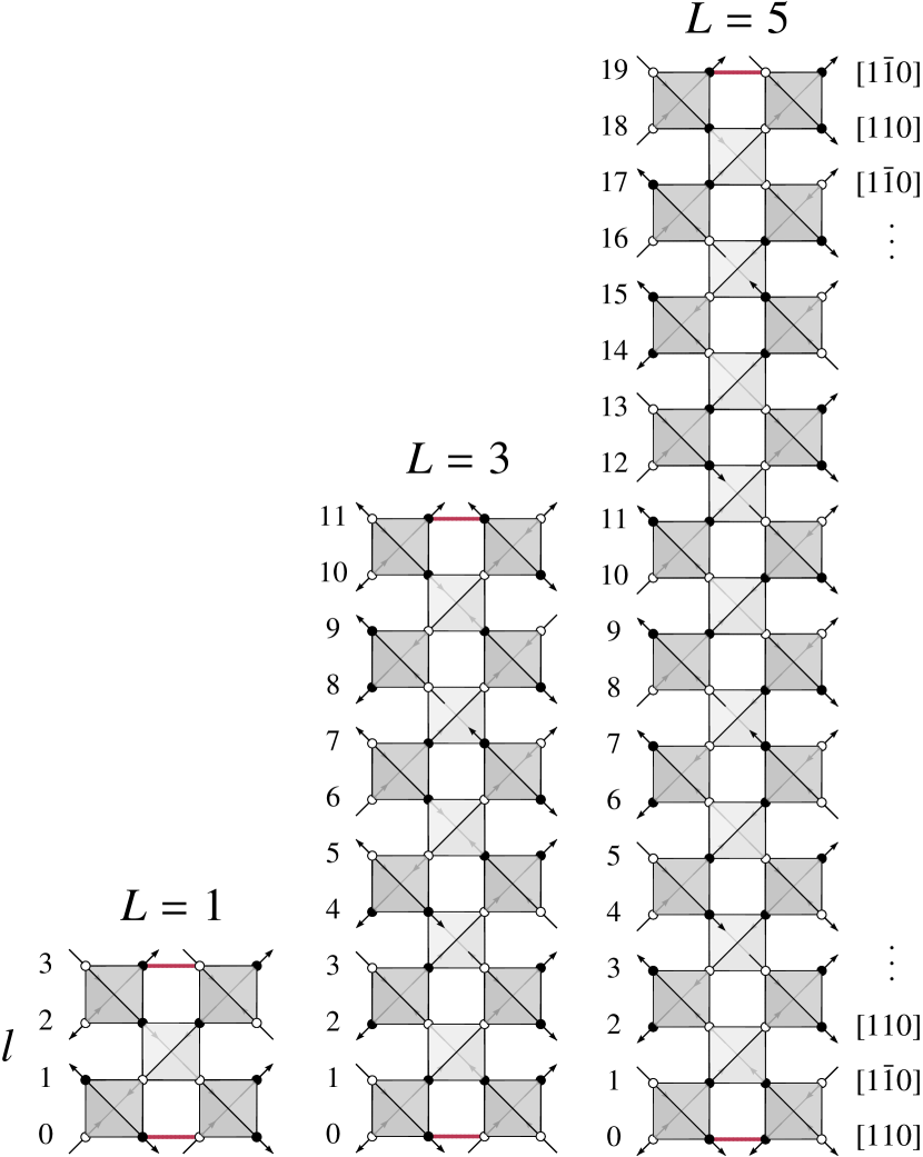
Figure 3: Structure of $[001]$ spin ice films for the three thicknesses discussed in the text ($L=1,3,5$). We show explicitly the layer index $l$ which runs from $l=0$ to $l=4L-1$ for a film of thickness $L$. Each layer contains two sublattices, $\alpha=2l,2l+1$, of the primitive cell of the film (see App. B). The one-dimensional chains that comprise each layer alternate between orientations $[110]$ and $[1\bar{1}0]$ from one layer to the next. Since the total number of layers, $4L$, is even, one surface has $[110]$ chains while the other has $[1\bar{1}0]$ chains.

As noted in Ref. [Jaubert et al., 2017], this cleaving renders some of the surface bonds locally inequivalent to those in the bulk. Generically, one expects the bonds that join the remaining spins of a cut-off tetrahedra, which we call orphan bonds following Ref. [Jaubert et al., 2017], to have an Ising coupling, $J_{\rm O}$, different than the other bonds in the film. We thus consider the following minimal model

$$H=J\sum_{\langle ij\rangle}\sigma_{i}\sigma_{j}+(J_{\rm O}-J)\sum_{\langle ij\rangle{\in\text{O}}}\sigma_{i}\sigma_{j},$$ (2)

where the first sum, $\langle ij\rangle$, runs over all NN bonds while the second sum, $\langle ij\rangle\in{\rm O}$, runs only over the orphan bonds .

III Methods

With our model of spin ice thin films defined, we now outline the methods used to tackle these systems. We first discuss the large-$N$ method and review its application to bulk spin ice. Next, we discuss the modifications needed for an application to spin ice thin films. Finally, we discuss the Monte Carlo methods used to simulate Ising ($N=1$) spin ice films directly.

III.1 Large-N method in bulk spin ice

The Hamiltonian for NN spin ice, Eq. (1), can be investigated using an analytically tractable approximation scheme, the so-called large-$N$ expansion. This method allows one to obtain semi-quantitative spin-spin correlation functions at low temperature Isakov et al. (2004). Consider the classical partition function, $\mathcal{Z}$, for the Hamiltonian in Eq. (1), written as

$$\mathcal{Z}=\sum_{\{\sigma_{i}\}=\pm 1}\exp\left\{-\frac{\beta J}{2}\sum_{ij}V_{ij}\sigma_{i}\sigma_{j}\right\},$$ (3)

where the sum over $i$ and $j$ runs over all pyrochlore lattice sites, and we have defined $V_{ij}=1$ when $i$ and $j$ are nearest-neighbors, and $V_{ij}=0$ otherwise. Replacing the classical Ising spins $\sigma_{i}$ by continuous variables $s_{i}$ and enforcing the unit spin length constraint leads to the partition function

$$\mathcal{Z}=\prod_{j}\int ds_{j}\ \delta(s_{j}^{2}-1)\exp\left\{-\frac{\beta J}{2}\sum_{ij}V_{ij}s_{i}s_{j}\right\}.$$ (4)

In this form, the length constraints render the partition function as intractable as the original model. The large-$N$ approach circumvents this problem by extending these real variables, $s_{i}$, to $N$-component vectors $\bm{s}_{i}$ subject to the constraint

$$|\bm{s}_{i}|^{2}=N.$$ (5)

The interaction between the spins is also extended to be $O(N)$ symmetric, with the resulting $\mathcal{Z}_{N}$ partition function now taking the form

$$\mathcal{Z}_{N}=\prod_{j}\int d\bm{s}_{j}\ \delta(|\bm{s}_{j}|^{2}-N)\exp\left\{-\frac{\beta J}{2}\sum_{ij}V_{ij}\bm{s}_{i}\cdot\bm{s}_{j}\right\}.$$ (6)

Clearly, if we set $N=1$, we recover the original Ising model with $\mathcal{Z}_{1}\equiv\mathcal{Z}$. The constraints at each site $i$ can be enforced using constraint fields $\mu_{i}$, so $\mathcal{Z}_{N}$ becomes

$$\int\mathcal{D}\bm{s}\mathcal{D}\mu\exp\left\{-\frac{1}{2}\sum_{j}i\mu_{j}\left(|\bm{s}_{j}|^{2}-N\right)-\frac{\beta J}{2}\sum_{ij}V_{ij}\bm{s}_{i}\cdot\bm{s}_{j}\right\},$$

where $\mathcal{D}\bm{s}\equiv\prod_{j}d\bm{s}_{j}$ and $\mathcal{D}\mu\equiv\prod_{j}d\mu_{j}$. Integrating out the $\bm{s}$ fields yields

$$\mathcal{Z}_{N}=\int\mathcal{D}\mu\exp\left\{-\frac{N}{2}{\rm Tr}\left[-i\mu+\log\left(i\mu+\beta JV\right)\right]\right\},$$ (7)

where we have defined the diagonal matrix $\mu$ with elements ${\mu}_{ij}\equiv\delta_{ij}\mu_{i}$. In this form, it is clear that as $N\rightarrow\infty$, the partition function is dominated by the saddle points of the exponential. In the saddle-point solutions, $\mu$ is purely imaginary, so we consider the real variable $\lambda\equiv i\mu$. The saddle-point equations are then given by

$$(\lambda+\beta JV)^{-1}_{ii}=1.$$ (8)

The correlation functions between the $\bm{s}_{i}$ can be readily obtained from Eqs. (6,7) by taking a derivative with respect to $V_{ij}$. One obtains

$$\langle s^{a}_{i}s^{b}_{j}\rangle=\delta_{ab}(\lambda+\beta JV)^{-1}_{ij},$$ (9)

where $a,b=1,\cdots N$ label the spin components. Note that by invoking this correlation function, the saddle-point condition can be interpreted as an average length constraint on the spins $\bm{s}_{i}$ with

$$\langle\bm{s}_{i}\cdot\bm{s}_{i}\rangle=N.$$ (10)

For bulk spin ice, the translation and rotation symmetries of the lattice enforce that the $\lambda_{i}$ are site independent with $\lambda_{i}\equiv\lambda_{0}$. We can then block diagonalize the interaction matrix $V$ using a Fourier transform which leads to

$$\langle{s^{a}_{\alpha}({\bm{q}})}^{*}s^{b}_{\beta}({\bm{q}})\rangle=\delta_{ab}\left[\lambda_{0}\bm{1}+\beta JV({\bm{q}})\right]^{-1}_{\alpha\beta},$$ (11)

where $\alpha,\beta=1,\dots,4$ index the four sublattices of the pyrochlore lattice, and the explicit form of the matrix $V(\bm{q})$ is given in App. A. The average length constraint [Eq. (10)] can then be expressed as

$$\frac{1}{n}\sum_{\alpha,{\bm{q}}}\langle{\bm{s}_{\alpha}({\bm{q}})}^{*}\cdot\bm{s}_{\alpha}({\bm{q}})\rangle=N.$$ (12)

where $n$ is the total number of spins in the system.

The previous derivation, leading to Eqs. (11) and (12), is equivalent (in outcome) to the so-called self-consistent Gaussian approximation or spherical approximation Stanley (1968). Perhaps surprisingly, this large-$N$ treatment has been found to provide semi-quantitative correlation functions when compared to Monte Carlo simulations of pyrochlore Ising ($N=1$) and Heisenberg ($N=3$) antiferromagnets Isakov et al. (2004). However, this method does not provide a good description of the physics for $N=2$ due to the manifestation of order-by-disorder Bramwell et al. (1994); Moessner and Chalker (1998a, b). In principle, a $1/N$ expansion Isakov et al. (2004) around this exactly solvable point would allow one to obtain more precise correlation functions for spins with finite $N$, but given the success of the $N\rightarrow\infty$ results, this seems unnecessary. The method has also been extended to include features found in more realistic models of spin ice; this includes further-neighbor exchange interactions Conlon and Chalker (2010); Silverstein et al. (2014) and dipolar interactions Sen et al. (2013).

III.2 Large-N method for spin-ice films

The application of the large-$N$ method to spin ice models in film geometries introduces additional complications to the methodology. In particular, the breaking of the translational symmetry in the finite direction of the film forbids a uniform constraint field, $\lambda_{0}$ (as is the case in bulk spin ice). However, one can still take advantage of the translational symmetry in the plane parallel to the surfaces, defining a constraint field on each layer $l$. Such layer-dependent constraint fields were used previously in Ref. Dantchev et al. (2014) to study Casimir effects in films of ferromagnets.

Proceeding as in the previous section, and integrating out the spin variables $\bm{s}_{i}$, we obtain the large-$N$ partition function

$$\mathcal{Z}_{N}=\int\mathcal{D}\lambda\exp\left\{-\frac{N}{2}{\rm Tr}\left[-\lambda+\log\left(\lambda+\beta JV\right)\right]\right\},$$ (13)

where the matrix $\lambda$ now has layer-resolved elements, $\lambda_{ij}=\lambda_{l}\delta_{ij}$, and the layer index $l$ is an implicit function of the lattice site $i$. Using the translational symmetry in the plane, the saddle-point solution [Eq. (10)] can be defined on each layer,

$$\frac{1}{n_{l}}\sum_{i\in l}\langle{\bm{s}_{i}\cdot\bm{s}_{i}}\rangle=N,$$ (14)

where $n_{l}$ is the number of spins on layer $l$. Spin-spin correlations in reciprocal space are obtained from Eq. (9) after performing a Fourier transform in the plane,

$$\bm{s}_{\alpha}(\bm{q}_{\perp}) =\frac{1}{\sqrt{n_{c}}}\sum_{\bm{r}}e^{-i(\bm{r}+\bm{r}_{\alpha})\cdot{\bm{q}_{\perp}}}\bm{s}_{\alpha}(\bm{r}),$$ (15)

where $\bm{r}$ runs over the $n_{c}$ primitive unit cells of the film, $\bm{q}_{\perp}$ are in-plane wave vectors, and $\bm{r}_{\alpha}$ are basis vectors locating each sublattice $\alpha$ within the unit cell. Note that we identified the pyrochlore lattice sites as $i\equiv(\mathbf{r},\alpha)$. One ultimately finds

$$\langle{s^{a}_{\alpha}({\bm{q}_{\perp}})}^{*}s^{b}_{\beta}({\bm{q}_{\perp}})\rangle=\delta_{ab}M^{-1}_{\alpha\beta}(\bm{q}_{\perp}),$$ (16)

where $M(\bm{q}_{\perp})\equiv\lambda+\beta JV(\bm{q}_{\perp})$, and $V(\bm{q}_{\perp})$ is the Fourier transform of the direct-space interaction matrix $V$. The numerical values of the constraint fields $\lambda_{l}$   are obtained by enforcing the saddle-point conditions, given in Eq. (14), which can be expressed as

$$\sum_{\alpha\in l}\sum_{\bm{q}_{\perp}}M^{-1}_{\alpha\alpha}(\bm{q}_{\perp})=n_{l},$$ (17)

for each layer $l$. We note that the framework provided by Eqs. (16) and (17) is completely general and does not suppose a particular choice of surface geometry, which appears in the definition of the unit cell and through the structure of the matrix $M(\bm{q}_{\perp})$. We also note that this analysis would carry through for spin ice films that include further-neighbor or dipolar interactions Jaubert et al. (2017), in their paramagnetic phases. One simply needs to compute the Fourier transform $V(\bm{q}_{\perp})$ of the corresponding interaction matrix in the chosen film geometry (see Refs. [Conlon and Chalker, 2010; Silverstein et al., 2014; Sen et al., 2013] for details in the bulk case). The inclusion of orphan bonds, as in Eq. (2), is also straightforward, with the corresponding interaction matrix $V(\bm{q})$ given in App. B.

III.3 Monte Carlo simulations

To confirm that the large-$N$ method correctly captures the physical behavior of the Ising ($N=1$) films at low temperatures, as it does in the bulk case Isakov et al. (2004), we perform a classical Monte Carlo simulation of the model of Eq. (2) for the appropriate film geometries. To avoid issues with equilibriation, we use a non-local Monte Carlo update. Specifically, we adapt the cluster algorithm of Ref. [Otsuka, 2014] to the film geometry. To implement the surfaces in the $[001]$ direction we consider a periodic system of cubic cells with dimensions $L_{\perp}\times L_{\perp}\times L$. This can be modified into the appropriate film geometry by cutting the bonds that pass through a plane with normal $\bm{\hat{z}}$ and changing the remaining two bonds to carry the orphan coupling, $J_{\rm O}$. This modifies the weights used for the surface tetrahedra in the cluster algorithm of Ref. [Otsuka, 2014], but otherwise leaves the algorithm unaffected for any choice of $J_{\rm O}/J$ (see App. D for further details). This cluster algorithm is closely related to the standard loop or worm algorithm used in spin ice simulations Melko et al. (2001); Melko and Gingras (2004), similar to the relationship between the Swensden-Wang Swendsen and Wang (1987) and Wolff Wolff (1989) cluster algorithms used in unfrustrated Ising models. For our purposes, one advantage of this formulation is the availability of an improved estimator Otsuka (2014) for the spin-spin correlation functions that allows to access larger system sizes at lower computational cost. Typically, accurate spin-spin correlations can be obtained with samples generated using only $10^{3}$ steps of the cluster algorithm when employing this improved estimator.

For the single-layer films ($L=1$), we considered systems up to $L_{\perp}=64$, while for the thicker films ($L=3$ and $L=5$) we considered sizes up to $L_{\perp}=32$. For a given system size $n=16L_{\perp}^{2}L$, we expect finite size effects to become important when the monopole density $\sim e^{-2J/T}$ Castelnovo et al. (2011) drops below $\sim 1/n$. Below the crossover temperature ${T}^{*}/J\sim 1/\log{n}$ one expects the system to be confined to the ice manifold itself and recover the $T=0$ behavior. For the lattice sizes of interest, the simulations become finite-size limited for temperatures less than ${T}^{*}/J\sim 0.1-0.2$. When considering the direct-space spin-spin correlators, we used smaller sizes of $L_{\perp}=16$, but with a larger number of samples, typically of order $10^{5}$, to ensure small statistical errors.

IV [001] spin ice films

To begin our exploration of spin ice films, we consider what is perhaps the simplest geometry: films with surfaces perpendicular to the $[001]$ crystallographic direction. We start with equivalent orphan and bulk bonds, $J_{\rm O}=J$, and then consider the more general and richer case, $J_{\rm O}\neq J$. In both cases, we apply the large-$N$ method described in Sec. III.2, and confirm its results via Monte Carlo simulations as described in Sec. III.3.

IV.1 Equivalent orphan and bulk bonds

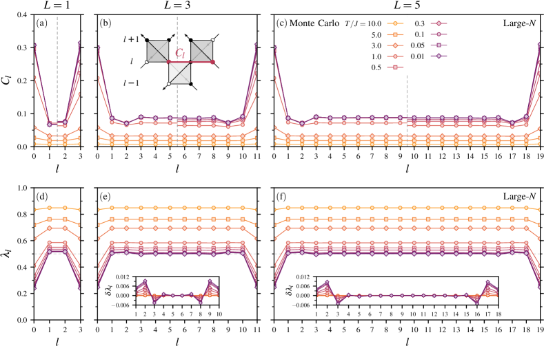
Figure 4: Layer-resolved real space correlations $C_{l}$ (a-c) [see the inset of (b) for a definition of $C_{l}$] and constraint fields $\lambda_{l}$ (d-f) of thin films of (a,d) 4 layers ($L=1$), (b,e) 12 layers ($L=3$) and (c,f) 20 layers ($L=5$), as a function of temperature $T/J$ and layer index $l$ (see Fig. 3). For the real space correlations the Monte Carlo result (left) is shown for a system size of $L_{\perp}=16$, while the large-$N$ results (right) are effectively in the thermodynamic limit ($L_{\perp}=\infty$). In panels (d-f), the dashed lines show the value $\lambda_{0}=1/2$ expected for bulk spin ice at $T/J=0$, and the insets show the deviation from the central layers, $\delta\lambda_{l}\equiv\lambda_{l}-\lambda_{2L}$.

We first consider films with the orphan bond coupling equal to that of the bulk ($J_{\rm O}=J$). We start with the thinnest films ($L=1$), where we expect the most pronounced effects when compared to the bulk case. To proceed, Eq. (17) must be solved numerically in order to obtain the set of constraint fields $\lambda_{l}$ as a function of $T/J$, which is needed to access all other observables. This is accomplished by applying the Newton-Raphson descent algorithm (see App. C). Although there are four spin layers, the symmetry of the slab leads to only two distinct constraint fields, as shown in Fig. 4(d). As $T/J\rightarrow 0$, the constraint fields for the middle layers approach the expected value for bulk spin ice, $\lambda_{0}=1/2$ Isakov et al. (2004), whereas the constraint fields for the surface layers converge to a significantly lower value. As a result, the in-plane spin-spin correlations acquire a layer-resolved character, with stronger correlations at the free surfaces than in the middle of the slab. As an example of this behavior, we show in Fig. 4(a) the direct space correlation function between second nearest neighbors on a given layer $l$, which we denote as $C_{l}$ [see inset of Fig. 4(b)]. We compute the same correlation function in the Monte Carlo simulations [see Fig. 4(a)] and find reasonable agreement.

To explore the fate of the key signature of the Coulomb phase, the presence of pinch points Henley (2005, 2010); Castelnovo et al. (2012), we consider the spin-spin correlation function, $S({\bm{q}})$, of the films in reciprocal space

$$S({\bm{q}})=\frac{1}{nN}\sum_{ij}\langle\bm{s}_{i}\cdot\bm{s}_{j}\rangle e^{i\bm{q}\cdot(\bm{r}_{i}-\bm{r}_{j})},$$ (18)

where $\bm{q}\equiv(\bm{q}_{\perp},q_{z})=2\pi(h\bm{\hat{x}}+k\bm{\hat{y}}+l\bm{\hat{z}})$ is a three-dimensional wave vector, expressed using Miller indices $[hkl]$. In terms of the spin-spin correlation matrix $M(\bm{q}_{\perp})$, we obtain

$$S({\bm{q}}) =\frac{1}{8L}\sum_{\alpha\beta}e^{iq_{z}(\bm{r}_{\alpha}-\bm{r}_{\beta})\cdot\bm{\hat{z}}}M_{\alpha\beta}^{-1}({\bm{q}_{\perp}}).$$ (19)

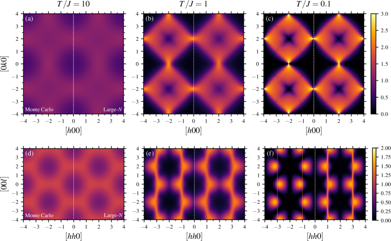
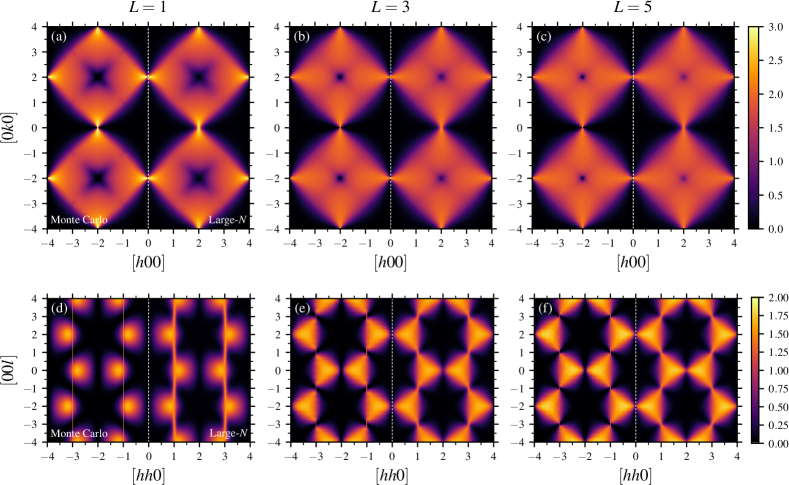
Figure 5: Spin-spin correlation functions, $S(\bm{q})$, [from large-$N$ (right) and Monte Carlo (left)] of spin ice films of thickness $L=1$, for temperatures (a,d) $T/J=10$, (b,e) $T/J=1$ and (c,f) $T/J=0.1$ in the (a-c) $[hk0]$ and (d-f) $[hhl]$ planes. Monte Carlo simulations were performed with $L_{\perp}=64$. For the temperatures considered, the large-$N$ results are (effectively) in the thermodynamic limit ($L_{\perp}\rightarrow\infty$).

Figure 6: Spin-spin correlation functions, $S(\bm{q})$, [from large-$N$ (right) and Monte Carlo (left)] of spin ice films of thickness (a,d) $L=1$, (b,e) $L=3$ and (c,f) $L=5$, for a temperature of $T/J=0.1$ in the (a-c) $[hk0]$ and (d-f) $[hhl]$ planes. Monte Carlo simulations were performed with $L_{\perp}=64$ (for $L=1$) and $L_{\perp}=32$ (for $L=3,5$). For $T/J=0.1$ the large-$N$ results are (effectively) in the thermodynamic limit ($L_{\perp}\rightarrow\infty$).

In Fig. 6, we show $S(\bm{q})$ for various temperatures $T/J$ in two high-symmetry planes: $[hk0]$ and $[hhl]$. Strikingly, the characteristic pinch-points remain intact in the $[hk0]$ scattering plane, parallel to the surfaces. However, as expected due to the finite extent in the $\bm{\hat{z}}$ direction, they are washed out in scattering planes with a non-zero $q_{z}$ component, normal to the film. We also observe “scattering rods” in the $q_{z}$ direction, and “secondary” pinch-points near $[110]$ and equivalent wave-vectors.

All these features are reproduced in Monte Carlo simulations for the same geometry. The only substantive difference between the Monte Carlo and large-$N$ results lies in the temperature dependence of the build up of spin-ice correlations, as found in the bulk case Isakov et al. (2004). For the large-$N$ case, due to the continuous nature of the spins, the correlation functions only approach the asymptotic $T=0$ result algebraically Henley (2005), while for discrete Ising spins this occurs exponentially . This can be seen explicitly in the pinch points; as $\sim\sqrt{T/J}\rightarrow 0$, their width decays as $\sim\sqrt{T/J}$ for the large-$N$ case, as compared to $\sim e^{-J/T}$ in the Monte Carlo simulations. This is most apparent in the $[hk0]$ plane, shown in Fig. 6(c) for $T/J=0.1$. In the Monte Carlo data, the pinch-point width is limited by the lateral system size $L_{\perp}$, while in the large-$N$ results there is an appreciable width. This difference in sharpness is also apparent in the width of the scattering rods in the $[hhl]$ plane [see Fig. 6(f)].

We now examine how the properties uncovered above change as the thickness is increased towards the bulk limit. Surprisingly, the numerical solution for the constraint fields $\lambda_{l}$ shows oscillations as a function of depth in the sample, as is illustrated in Fig. 4(e,f) for films with $L=3$ and $L=5$. These oscillations have increasing amplitude with decreasing temperature and a characteristic damping length scale which appears independent of thickness, indicative of a surface effect. They are also seen in the layer-resolved direct-space correlations $C_{l}$ and are well reproduced in the Monte Carlo simulations, as shown in Fig. 4(b,c), keeping in mind the difference in temperature dependence expected between the large-$N$ theory and the Ising model. We have verified that a large-$N$ treatment of thin films of a pyrochlore Ising ferromagnet [i.e. Eq. (1) with $J\rightarrow-J$] with the same geometry does not show oscillations in the constraint fields $\lambda_{l}$, but rather a monotonic behavior from the surface to the middle of the sample, as long as the system remains in the high-temperature paramagnetic phase. These results thus suggest that the oscillations are directly related to the geometrical frustration.

We also compute the spin-spin correlation functions $S(\bm{q})$ [given by Eq. (19)] at $T/J=0.1$, deep in the Coulomb phase, for thicknesses of $L=1,3$ and $5$ (see Fig. 6). In the $[hk0]$ plane, pinch-points are always present, with an increased contrast for thinner films. In the $[hhl]$ plane, the washed-out pinch-points are progressively restored with increasing thickness, as the system crosses over from a two-dimensional to three-dimensional Coulomb phase. The restoration of the “three-dimensional” pinch-points in the $[hhl]$ plane is set by the thickness of the film $L$ which cuts off the Coulomb correlations in the $\bm{\hat{z}}$ direction. Roughly, we expect quasi-two-dimensional behaviour when the correlation length, $\xi\sim e^{J/T}$, becomes of the order of the film thickness, $L$, giving a crossover temperature $T\sim J/\log{L}$. As with the $L=1$ films and bulk results, the Monte Carlo and large-$N$ results agree well, aside from the aforementioned temperature dependence (algebraic compared to exponential) of the build up of Coulomb correlations.

IV.2 Inequivalent orphan and bulk bonds

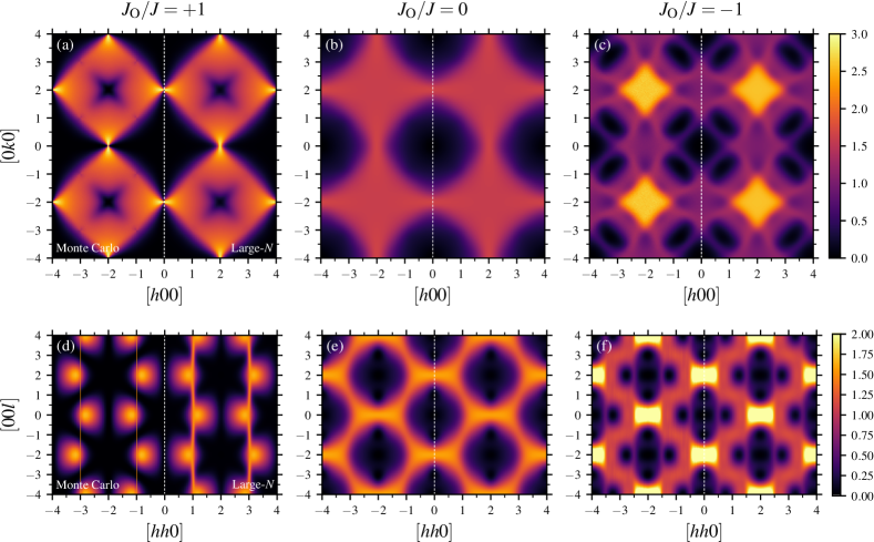
Figure 7: Spin-spin correlation functions, $S(\bm{q})$, [from large-$N$ (right) and Monte Carlo (left)] of spin ice films of thickness $L=1$ and temperature $T/J=0.1$ in the (a-c) $[hk0]$ and (d-f) $[hhl]$ planes. Orphan bond values of (a,d) $J_{\rm O}/J=1$, (b,e) $J_{\rm O}/J=0$ and (c,f) $J_{\rm O}/J=-1$ are shown. Monte Carlo simulations were performed with $L_{\perp}=64$ for all $J_{\rm O}/J$. For $T/J=0.1$ the large-$N$ results are (effectively) in the thermodynamic limit ($L_{\perp}\rightarrow\infty$).

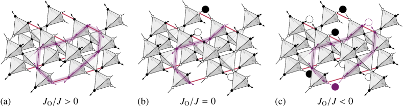
Figure 8: Representative ground states of $L=1$ $[001]$ films with $J_{\rm O}/J=+1,0,-1$. (a) When $J_{\rm O}/J>0$, the orphan-bond spins are anti-aligned, so that the flux lines run parallel to the surfaces. (b) When $J_{\rm O}=0$, no specific configuration of the orphan bond spins is preferred, so that half of the orphan bonds (on average) host surface charges. (c) When $J_{\rm O}/J<0$, the orphan-bond spins are aligned, leading to surface charges at the endpoints of flux lines. In cases (b,c), these fluctuating charges destroy the Coulomb phase and its associated pinch points. For each case we highlight a group of spins that can be flipped at zero energy cost.

We now move to the more general case and consider the influence of differing orphan and bulk bonds ($J_{\rm O}\neq J$), as defined in Eq. (2), on the physics of NN spin ice films. At low temperature ($T\ll|J_{\rm O}|,J$), we find that the system remains paramagnetic with the physics depending only on the sign of $J_{\rm O}$ (not on its magnitude). This is expected because the “bulk” ice rules are always compatible with minimizing the energy of the orphan bonds. We show the spin-spin correlations function, $S(\bm{q})$, for three representative values $J_{\rm O}/J=+1,0,-1$ in Fig. 7. The case $J_{\rm O}/J=1$ corresponds to the results of the previous section, with sharp pinch points characteristic of a two-dimensional Coulomb phase. However, these pinch points completely disappear for $J_{\rm O}/J=0$ and $J_{\rm O}/J=-1$, revealing only broad features in $S(\bm{q})$ in the low-temperature regime.

The preservation or destruction of the Coulomb phase (depending on the sign of $J_{\rm O}/J$) can be understood in terms of a simple picture of the ground state manifold for arbitrary film thicknesses. Note that for $J_{\rm O}/J>0$, the flux lines of the field $\bm{B}$ (see Sec. II.1) run along the surface and are then redirected back into the bulk of the film [see 8(a)]. This choice of orphan bond coupling is thus compatible with the (bulk) constraint $\bm{\nabla}\cdot\bm{B}=0$ and the Coulomb phase, now two-dimensional, is preserved. However, as discussed in Ref. [Jaubert et al., 2017], when $J_{\rm O}/J<0$, the orphan bonds host pairs of aligned spins which correspond to surface magnetic charges. These surface charges serve as endpoints to the “flux-lines” of the effective magnetic field $\bm{B}$ [see Fig. 8(c)]. Just as a finite density of thermally populated monopoles endows the pinch points in bulk spin ice with a finite width Henley (2010); Castelnovo et al. (2011), the finite density of these fluctuating surface charges broaden the pinch points in spin ice films. However, unlike the bulk case, these charges are present even at $T=0$ and thus destroy the Coulomb phase. We note that the destruction of the Coulomb phase is ultimately averted in Ref. Jaubert et al. (2017) by the ordering of the surface charges due to the long-range dipolar interactions. This static ordering inhibits thermal fluctuations of the surface charges and restores the two-dimensional Coulomb phase below the ordering temperature – a behavior reminiscent of magnetic fragmentation Brooks-Bartlett et al. (2014). In other words, the state we find for $J_{\rm O}/J<0$ can be viewed as the “parent” state out of which the ordering of Ref. [Jaubert et al., 2017] arises.

Finally, we consider the special case $J_{\rm O}/J=0$. Since the orphan bonds provide no energetic constraint, their spin configuration is essentially random. This leads to both the presence and absence of surface charges, as illustrated in Fig. 8(b). The finite density of these surface charges, while not maximal (as for $J_{\rm O}/J<0$), is sufficient to destroy the Coulomb phase. This results in the absence of pinch points in $S(\bm{q})$, as observed in Fig. 7(b).

We have verified that when $L$ is increased, the spin-spin correlation functions $S(\bm{q})$ approach the bulk result for any $J_{\rm O}/J$ (not shown). In particular, the gradual recovery of the pinch-points indicates that algebraic correlations are present up to a length scale set by the film thickness, $L$, even in the presence of surface charges. As mentioned above, this is analogous to the case of thermally activated charged defects (monopoles) in bulk spin ice which cut off the algebraic correlations at a length scale set by their average separation Castelnovo et al. (2011). We have also investigated the depth dependence of the constraint fields $\lambda_{l}$ and the layer-resolved correlators $C_{l}$; we find that these oscillate as a function of layer index $l$ (for $L>1$) for all values of $J_{\rm O}/J$ considered (not shown).

V Classical topological order in [001] films

The previous section has exposed, via large-$N$ and Monte Carlo results, how boundary conditions affect the Coulomb phase present in the parent bulk system. In this section, we relate these results to the topological order that characterizes different classical spin liquids Jaubert et al. (2013); Rehn et al. (2017). In particular, we argue that the low-temperature state of films with $J_{\rm O}/J<0$, while not a Coulomb phase, is nonetheless a non-trivial collective paramagnet – a classical $Z_{2}$ spin liquid Rehn et al. (2017).

First recall that in bulk spin ice, the spins can be mapped to dimers on the dual diamond lattice Hermele et al. (2004). Specifically, we identify $\sigma=+1$ with the presence of a dimer on the corresponding bond of the diamond lattice (similarly, $\sigma=-1$ is identified with the absence of such a dimer). The ice rules then correspond to the requirement that two dimers touch at each diamond lattice site. To move within the ice manifold, one uses “loop moves” that reverse all the spins on an alternating spin loop Melko et al. (2001); Melko and Gingras (2004). In the dimer picture, this corresponds to swapping the occupied and unoccupied bonds on this loop. Any “short” loop (not spanning the system) thus preserves three winding numbers, corresponding to the number of dimers crossing three planes oriented in the $\bm{\hat{x}}$, $\bm{\hat{y}}$ or $\bm{\hat{z}}$ directions. These winding numbers are topological invariants that characterize the classical $U(1)$ spin liquid (Coulomb phase), and can only be changed by “large” loops that wind around the periodic directions of the system .

How does this physics change for films? First, since our system is two-dimensional, we can define at most two distinct winding numbers. Second, in addition to the usual “bulk” loop moves, we can also construct zero-cost moves that involve the surface spins. When $J_{\rm O}/J>0$, the constraint of anti-aligned orphan bond spins only allows the construction of loops that run along the orphan bonds, as shown in Fig. 8(a). The two in-plane winding numbers thus remain topological invariants and we have a two-dimensional Coulomb phase, a classical $U(1)$ spin liquid.

The $J_{\rm O}/J<0$ case is more interesting. Here, to construct a zero-cost move, we must consider open strings of alternating spins that end in pairs on the orphan bonds, since preserving the surface constraint requires flipping both orphan bond spins. One can view such a pair of strings as a usual loop, where the alternation pattern is reversed when an orphan bond is encountered [see Fig. 8(c)]. Therefore, contributions from the two strings add up, and these moves can change the winding numbers only by even amounts, leading to the destruction of the aforementioned classical $U(1)$ topological order. However, not all is lost; one can still define two $Z_{2}$ topological invariants Rehn et al. (2017), corresponding to the two “winding parities”, that can only be changed by moves that wrap around the system. This leads us to identify the paramagnetic phase found for $J_{\rm O}/J<0$ films as a classical $Z_{2}$ spin liquid, consistent with the absence of pinch-points exposed in Sec. IV . A direct consequence of such (classical) $Z_{2}$ topological order is the predicted presence of fractionalized magnetic moments bound to vacancies in the film Rehn et al. (2017).

Finally, we turn to the $J_{\rm O}/J=0$ case. At this point the system is neither a $Z_{2}$ nor a $U(1)$ spin liquid. We can see this noting that strings of alternating spins terminating on the orphan bonds can be flipped at zero energy cost [see Fig. 8(b)]. Flipping these strings can change the winding numbers arbitrarily, even for short strings. We thus conclude that the $J_{\rm O}/J=0$ case does not support topological sectors. Given that this case sits at the critical point between the $U(1)$ and $Z_{2}$ spin liquids, its properties have more general implications for the regime where $|J_{\rm O}|\ll T\ll J$. In this limit, the orphan bonds are effectively at high temperature, so the system will behave more like the $J_{\rm O}/J=0$ point, rather than the classical $U(1)$ or $Z_{2}$ spin liquids (see the phase diagram in Fig. 2).

VI Magnetically charged surfaces in [110] and [111] films

In the previous section, we showed how specific boundary conditions (the orphan bond exchange $J_{\rm O}$) have, through the formation of fluctuating surface charges, dramatic effects on the properties of the film. With an understanding of the “simple” case of $[001]$ films, we now proceed to briefly discuss more complicated geometries, specifically films with surfaces perpendicular to the $[110]$ and $[111]$ directions. These geometries are obtained by cutting one (or three) spins per surface tetrahedron, as shown in Fig. 9. The resulting slab is comprised of alternating kagome and triangular layers for $[111]$ films, but has a somewhat more complicated geometry for $[110]$ films.

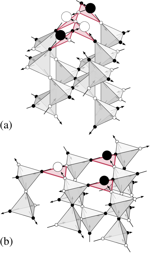
Figure 9: Representative ground states of films cleaved along the (a) $[110]$ or (b) $[111]$ directions. In both cases, the cleaving shown cuts one spin per surface tetrahedron, leaving orphan triangles at the surface. Flux lines are therefore required to have endpoints on each of these orphan triangles, leading to surface charges irrespective of the sign of $J_{\rm O}/J$.

These two geometries differ drastically from the $[001]$ films which, having two spins remaining per surface tetrahedron, can still (in principle) respect the divergence-free condition $\bm{\nabla}\cdot\bm{B}=0$ defining the Coulomb phase, by having one spin pointing in and one pointing out. Whether this is energetically favorable depends on the value of $J_{\rm O}/J$, as explained in Sec. IV. This is, however, impossible for $[110]$ or $[111]$ spin ice films, where the surface tetrahedra have either one or three spins remaining – in other words, the boundary conditions imposed on the $\bm{B}$ field at the surfaces are fundamentally incompatible with the divergence-free condition of the bulk. As a result, the surface tetrahedra must host a charge of the $\bm{B}$ field, irrespective of the value of $J_{\rm O}/J$, as illustrated in Fig. 9. In $[110]$ films, these effective magnetic charges sit on parallel “zig-zag” chains running on the surfaces [see Fig. 9(a)], whereas in $[111]$ films, they live on a triangular lattice [see Fig. 9(b)]. As discussed in Sec. IV, when these charges can fluctuate, they serve as free, zero-cost end-points for the (effective) magnetic flux lines. The presence of such zero-cost end points will generically destroy the two-dimensional Coulomb correlations. We thus expect any two-dimensional pinch-points to be destroyed for $[111]$ or $[110]$ films.

However, we do not expect a classical $Z_{2}$ spin liquid in these geometries. For $J_{\rm O}/J>0$, the surface monopoles are at the end of only one flux line. Thus, there is no constraint on changes of the winding numbers incurred by local updates. In contrast, for $J_{\rm O}/J<0$ the surface triangles consist of three aligned spins, and thus three strings must terminate at each triangle. Borrowing the arguments of Sec. V, this would imply the presence of a classical $Z_{3}$ spin liquid Motrunich (2003); Rehn et al. (2016) as the winding numbers can only change in multiples of three. Whether the physics discussed above extends to zero temperature, or is preempted by some ordering phenomena requires detailed numerical study, which we leave to future work.

While this picture of surface charges applies to the Ising case ($N=1$), the $N\geq 3$ cases should be qualitatively different. Consider as an example a $[111]$ film terminating on a kagome layer; while three Ising spins cannot add to zero on orphan triangles, thus requiring surface charges, three $N=3$ (or higher) vectors can sum to zero. This implies that such surface charge defects (i.e. a non-zero sum of spins) are not required for the $N=3$ (or higher) case. We thus expect that for $[110]$ and $[111]$ films with orphan triangles, the large-$N$ result will be qualitatively different than the Ising case, with the two-dimensional Coulomb phase not (necessarily) destroyed .

VII Discussion

We now discuss some potential extensions and implications of our work. In particular, we outline applications to continuous spin systems, possible extensions to dipolar spin ice films and the surfaces of bulk single crystal dipolar spin ices. In addition, we speculate on more theoretical aspects, such as the effects of a magnetic field and the physics of quantum spin ice films Gingras and McClarty (2014).

In view of making concrete contact with experimental realizations, we discuss some aspects of films of spin ice materials. There are several complications in connecting the ideas discussed in this work to the physics of these compounds. First, crystal symmetry breaking at the interface between spin ice and vacuum could weaken or even destroy the Ising nature of the spins and their interactions Rau and Gingras (2015) near the surfaces. For canonical spin ices such as Dy₂Ti₂O₇ and Ho₂Ti₂O₇, this may not be a serious concern. Since the crystal field ground doublets of Dy- and Ho-based pyrochlores are predominantly maximal-rank (mostly $J_{z}=\pm 15/2$ and $J_{z}=\pm 8$ respectively), strong perturbations to the crystal field would be necessary to generate significant effects on the single-ion or two-ion properties Rau and Gingras (2015). One might then expect that the induced transverse (quantum) exchange at the surfaces would be small for both compounds and that the splitting of the non-Kramers doublet expected in Ho₂Ti₂O₇ might be negligible. For the case of the Pr₂M₂O₇ family mentioned in Sec. II, these effects are likely to be more drastic. Indeed, the presence of large random transverse fields Wen et al. (2017) due to weak structural disorder appears to be a feature even in bulk samples. Given that the crystal field doublet in these non-Kramers compounds lacks the “axial protection” present in Ho₂Ti₂O₇ Rau and Gingras (2015), we expect these transverse fields to be further enhanced at any surfaces. These complications could be minimized through more clever engineering of the films. For example, one might consider heterostructures composed of a thin layer of a spin ice material sandwiched between layers of non-magnetic pyrochlore materials having the same crystal structure and similar lattice constant, such as La₂M₂O₇, Lu₂M₂O₇ and Y₂Ti₂O₇.

However, one serious difficulty with all of the proposals for spin ice thin films and heterostructures is the effect of substrate-induced strain. This could be due to a lattice constant mismatch, or simply to slight chemical bonding differences at the interface. The presence of such strain will generically strengthen some of the bonds and remove the ground state degeneracy and residual entropy Jaubert et al. (2010, 2017). In non-Kramers compounds, this could also induce a transverse field at each site (depending on the film geometry and strain direction); as in the case of surfaces, this could be negligible for Ho₂Ti₂O₇, but significant in the Pr₂M₂O₇ family. How this strain can be minimized, so that the intrinsic physics of spin ice films can be exposed, is an important but exciting challenge in the fabrication of these systems.

In dipolar spin ice such as Dy₂Ti₂O₇ or Ho₂Ti₂O₇, the long-range tail of dipolar interactions should have significant effects on the physics discussed here. For bulk spin ice, these differences are suppressed due to the structure of the spin-ice manifold – the dipolar interactions are effectively short-range when acting on ice states Gingras and den Hertog (2001); Isakov et al. (2005); this is the so-called self-screening or projective equivalence. Consequently, the splitting of the ice manifold is small, and the associated ordering due to the dipolar interactions only occurs at low temperature compared to the bare scale of the dipolar interactions Melko et al. (2001). However, when monopoles or surface charges are present, the dipolar interaction is significant, promoting the entropic Coulomb interaction between the defects into an energetic one. Indeed, it was found in Ref. [Jaubert et al., 2017] that for $[001]$ surfaces with ferromagnetic orphan bonds, this attraction induces a phase transition to long-range order of the surface charges into a checkerboard pattern. For films with $[110]$ or $[111]$ surfaces, the analogous physics is likely to be even richer. For example, in the $[111]$ geometry, the charges live on a triangular lattice, with either a single monopole or anti-monopole at each site. While each surface is not required to be neutral (due the presence of the other surface), this will be favored energetically. One thus expects a one-component Coulomb gas at half-filling (the other component being treated as background) on a triangular lattice. At the nearest neighbor level, this is equivalent to an anti-ferromagnetic triangular lattice Ising model and is highly frustrated, with a macroscopically degenerate set of ground states Wannier (1950). The effective long-range Coulomb interactions will presumably lift this degeneracy but, as in dipolar spin ice, only weakly, due to the approximate local charge neutrality.

Some of the physics discussed here is expected to carry over from the thin film context to that of exposed surfaces of bulk crystals of spin ice materials. For example, the presence of fluctuating surface charges in certain geometries may have screening effects on the fields from monopoles in the bulk.

As discussed in Sec. VI, the physics of different surface terminations depends strongly on the nature of the spins in question. While we have mainly discussed Ising spins here, it is known that the large-$N$ method also works well for $O(3)$ spins Isakov et al. (2004); Conlon and Chalker (2010). Examples of pyrochlore anti-ferromagnets with such continuous, classical spins include certain spinels Lee et al. (2010), as well as the recently discovered chemically disordered fluorine pyrochlores Krizan and Cava (2014, 2015). Thin films of such compounds may be an interesting playground to explore analogues of the physics discussed in this work. Other interesting avenues in this direction include the case of $O(2)$ spins, where the large-$N$ method is known to be unreliable due to the appearance of order-by-disorder Bramwell et al. (1994); Moessner and Chalker (1998b, a). Experimentally, there are several promising candidates; for example the bulk XY pyrochlores are known to exhibit rather exotic behaviors, from the order-by-disorder physics of Er₂Ti₂O₇ Champion et al. (2003); Zhitomirsky et al. (2012); Savary et al. (2012) to the unusual physics of the Yb₂M₂O₇ family, Yb₂Ge₂O₇ in particular Dun et al. (2014, 2015); Hallas et al. (2016) (see Ref. [Hallas et al., 2018] for a review). Further, the limit of an anti-ferromagnetic XY model has been found to harbor several exotic phases, including a spin liquid at intermediate temperature and a “hidden” quadrupolar order at low temperature Taillefumier et al. (2017); the effect of a film geometry would likely lead to rich physics.

On the more theoretical front, there are many fundamental open questions about spin ice films. For example, bulk spin ice shows a complex phase diagram in an external magnetic field, with the physics strongly dependent on the field direction Moessner and Sondhi (2003); Jaubert et al. (2008); Ruff et al. (2005); the effect of magnetic fields on films is likely to be similarly rich. The effects of transverse exchange also raises a host of interesting questions: in bulk spin ice this induces tunnelling between the ice states and stabilizes a $U(1)$ quantum spin liquid, quantum spin ice Gingras and McClarty (2014). However, the quantum analogue of the two dimensional Coulomb phase is fundamentally unstable Polyakov (1977), meaning that a direct two-dimensional analogue of quantum spin ice does not exist Henry and Roscilde (2014). The fate of quantum spin ice films is thus unclear; possibilities include magnetically ordered states, valence bond solids Henry and Roscilde (2014) or potentially a quantum $Z_{2}$ spin liquid, as found in related models on the kagome lattice Carrasquilla et al. (2015). How the resulting state in this quantum case depends on the film geometry and the choice of orphan bond exchange presents many directions to pursue in future studies. Given the ability to readily grow high quality rare-earth pyrochlore oxide films Leusink et al. (2014); Bovo et al. (2014), one might expect such theoretical investigations to motivate a range of experimental studies which will, in return, undoubtedly fuel new sets of theoretical questions.

The study of films of pyrochlore magnets is a nascent field with many open questions, and rapid development could be expected in the near future. We our hope that this work will help shed light onto these systems and provide guidance and motivation for upcoming experimental and theoretical work.

Appendix A Bulk spin ice

A.1 The pyrochlore lattice

The pyrochlore lattice is a face-centered cubic lattice decorated with a tetrahedron at each site. We take the conventional cubic unit cell of side length $a=1$; in this convention the nearest neighbor distance is $r_{\rm nn}=\sqrt{2}/4$. The primitive unit cell is an upwards-tetrahedron, with four sublattice sites located at each vertex, with the following sublattice vectors:

$$\bm{r}_{0} =\bm{0}, \bm{r}_{1} =\frac{\bm{\hat{x}}+\bm{\hat{y}}}{4}, \bm{r}_{2} =\frac{\bm{\hat{x}}+\bm{\hat{z}}}{4}, \bm{r}_{3} =\frac{\bm{\hat{y}}+\bm{\hat{z}}}{4}.$$ (20)

The local quantization axes for spin ice are defined with respect to the primitive unit cell,

$$\bm{\hat{z}}_{0} =\frac{\bm{\hat{x}}+\bm{\hat{y}}+\bm{\hat{z}}}{\sqrt{3}}, \bm{\hat{z}}_{1} =\frac{\bm{\hat{z}}-\bm{\hat{x}}-\bm{\hat{y}}}{\sqrt{3}},$$

$$\bm{\hat{z}}_{2} =\frac{\bm{\hat{y}}-\bm{\hat{z}}-\bm{\hat{x}}}{\sqrt{3}}, \bm{\hat{z}}_{3} =\frac{\bm{\hat{x}}-\bm{\hat{y}}-\bm{\hat{z}}}{\sqrt{3}},$$ (21)

where the indexing matches that of the sublattice vectors.

A.2 Interaction matrix

The explicit form of the interaction matrix $V(\bm{q})$ for NN bulk spin ice is

$$V({\bm{q}})=A({\bm{q}})+2\bm{1}_{4\times 4},$$ (22)

where the term proportional to the identity matrix makes the Lagrange multiplier $\lambda$ in the large-$N$ theory $\lambda$ consistent with the stiffness parameter of the Coulomb phase. The so-called adjacency matrix $A(\bm{q})$ is given by

$$A(\bm{q})=2\begin{pmatrix}0&c_{01}&c_{02}&c_{03}\\ c_{10}&0&c_{12}&c_{13}\\ c_{20}&c_{21}&0&c_{23}\\ c_{30}&c_{31}&c_{32}&0\end{pmatrix},$$ (23)

where $c_{\alpha\beta}\equiv\cos[\bm{q}\cdot(\bm{r}_{\alpha}-\bm{r}_{\beta})]$.

Appendix B [001] Films

B.1 Unit cell

For films with surfaces perpendicular to the $[001]$ direction, we use a primitive unit cell spanning the whole finite ($\bm{\hat{z}}$) direction, with $8L$ sublattices, where $L$ is the number of cubic (conventional) unit cells in the finite direction. The primitive lattice vectors are

$$\bm{a}_{1} =\bm{\hat{x}}, \bm{a}_{2} =\frac{\bm{\hat{x}}+\bm{\hat{y}}}{2},$$ (24)

and the sublattice vectors $\bm{r}_{\alpha}$ are given by

$$\bm{r}_{0} =\bm{0}, \bm{r}_{1} =\frac{\bm{\hat{x}}+\bm{\hat{y}}}{4},$$

$$\bm{r}_{2} =\frac{\bm{\hat{x}}+\bm{\hat{z}}}{4}, \bm{r}_{3} =\frac{\bm{\hat{y}}+\bm{\hat{z}}}{4},$$

$$\bm{r}_{4} =\frac{2\bm{\hat{x}}+2\bm{\hat{z}}}{4}, \bm{r}_{5} =\frac{3\bm{\hat{x}}+\bm{\hat{y}}+2\bm{\hat{z}}}{4},$$

$$\bm{r}_{6} =\frac{3\bm{\hat{x}}+3\bm{\hat{z}}}{4}, \bm{r}_{7} =\frac{2\bm{\hat{x}}+\bm{\hat{y}}+3\bm{\hat{z}}}{4},$$ (25)

for the first eight spins, and $\bm{r}_{\alpha+8k}=\bm{r}_{\alpha}+k\bm{\hat{z}}$, $k=1,..,L-1$ for the remaining spins. The corresponding conventional unit cell, showing the structure of stacked layers in the $\bm{\hat{z}}$ direction (each layer made of parallel chains in the $[110]$ or $[1\bar{1}0]$ direction, alternatively) is shown in Fig. 3.

B.2 Interaction matrix

Similar to the bulk theory, we define

$$V(\bm{q}_{\perp})=A(\bm{q}_{\perp})+2\bm{1}_{8L\times 8L}.$$ (26)

The adjacency matrix $A(\bm{q}_{\perp})$ is a $8L\times 8L$ matrix with a tridiagonal $8\times 8$ block structure – that is, only the diagonal blocks and next-to-diagonal blocks are non-trivial. For spins in the same cubic unit cell, the diagonal $8\times 8$ block reads

$$A_{\rm diag}(\bm{q}_{\perp})=\begin{pmatrix}0&2c_{01}&e_{02}&e_{03}&0&0&0&0\\ 2c_{10}&0&e_{12}&e_{13}&0&0&0&0\\ e_{20}&e_{21}&0&2c_{23}&e_{24}&e_{25}&0&0\\ e_{30}&e_{31}&2c_{32}&0&e_{34}&e_{35}&0&0\\ 0&0&e_{42}&e_{43}&0&2c_{45}&e_{46}&e_{47}\\ 0&0&e_{52}&e_{53}&2c_{54}&0&e_{56}&e_{57}\\ 0&0&0&0&e_{64}&e_{65}&0&2c_{67}\\ 0&0&0&0&e_{74}&e_{75}&2c_{76}&0\end{pmatrix},$$ (27)

where $e_{\alpha\beta}\equiv\exp[i\bm{q}_{\perp}\cdot\bm{r}_{\alpha\beta}]$, and $\bm{r}_{\alpha\beta}$ is the nearest-neighbor vector connecting sublattices $\alpha$ and $\beta$. The next-to-diagonal $8\times 8$ blocks are given by:

$$A(\bm{q}_{\perp})_{\text{upper}}=\begin{pmatrix}0&0&\cdots&0\\ \vdots&\vdots&\ddots&0\\ 0&0&\cdots&0\\ e_{60}&e_{61}&\cdots&0\\ e_{70}&e_{71}&\cdots&0\end{pmatrix},$$ (28)

$$A(\bm{q}_{\perp})_{\text{lower}}=\begin{pmatrix}0&\cdots&0&e_{06}&e_{07}\\ 0&\cdots&0&e_{16}&e_{17}\\ \vdots&\ddots&0&0&0\\ 0&\cdots&0&0&0\end{pmatrix}.$$ (29)

One can check that the complete adjacency matrix $A(\bm{q})$ is indeed Hermitian. All other couplings are zero.

B.3 Including orphan bonds

When including orphan bonds, with an Hamiltonian given by Eq. (2), the interaction matrix becomes

$$V(\bm{q}_{\perp})=A(\bm{q}_{\perp})+2\bm{1}_{8L\times 8L}+\left(\frac{J_{\rm O}-J}{J}\right)A_{\text{O}}(\bm{q}_{\perp}),$$ (30)

where the adjacency matrix corresponding to the orphan bond couplings, $A_{\text{O}}(\bm{q}_{\perp})$, has only the following non-zero matrix elements:

$$A_{\text{O}}(\bm{q}_{\perp})_{01} =\exp[-i\bm{q}_{\perp}\cdot(\bm{r}_{0}-\bm{r}_{1})],$$

$$A_{\text{O}}(\bm{q}_{\perp})_{10} =\exp[+i\bm{q}_{\perp}\cdot(\bm{r}_{0}-\bm{r}_{1})],$$

$$A_{\text{O}}(\bm{q}_{\perp})_{8L-2,8L-1} =\exp[-i\bm{q}_{\perp}\cdot(\bm{r}_{6}-\bm{r}_{7})],$$

$$A_{\text{O}}(\bm{q}_{\perp})_{8L-1,8L-2} =\exp[+i\bm{q}_{\perp}\cdot(\bm{r}_{6}-\bm{r}_{7})].$$ (31)

Appendix C Numerical solution of saddle-point equations

Here we briefly describe the method used to numerically solve Eq. (17):

$$\sum_{\alpha\in l}\sum_{\bm{q}_{\perp}}M^{-1}_{\alpha\alpha}({\bm{q}}_{\perp})=n_{l},$$ (32)

for each layer $l$. First, let us remark that the matrix $M(\bm{q}_{\perp})$ is not block-diagonal. Therefore, the spin-spin correlation matrix $M^{-1}(\bm{q}_{\perp})$ has diagonal elements that, in general, couple all coefficients $\lambda_{l}$ with $l~{}=~{}1,\>...\>,4L$. This means that one has to solve numerically for all the $4L$ self-consistent equations simultaneously.

We use the Newton-Raphson descent method, which allows one to find the zeros of a real-valued function. Consider

$$f_{l}(\bm{\Lambda})\equiv n_{l}-\sum_{\alpha\in l}\sum_{\bm{q}_{\perp}}M^{-1}_{\alpha\alpha}(\bm{q}_{\perp},\bm{\Lambda}),$$ (33)

where $\bm{\Lambda}~{}=~{}(\lambda_{1},\lambda_{2},...,\lambda_{4L})$. We wish to solve $\bm{f}(\bm{\Lambda})~{}=~{}\bm{0}$, with $\bm{f}=(f_{1},f_{2},...,f_{4L})$. We start with an initial configuration $\bm{\Lambda}^{(0)}$, chosen so that the eigenvalues of $M(\bm{q}_{\perp},\bm{\Lambda}^{(0)})$ are positive, iterating the configuration from step $n$ to step $n+1$ using

$$\bm{\Lambda}^{(n+1)}=\bm{\Lambda}^{(n)}-D^{-1}\cdot\bm{f}(\bm{\Lambda}^{(n)}),$$ (34)

where $D$ is the Jacobian matrix with elements

$$D_{ij}=\left[\frac{\partial f_{i}}{\partial\lambda_{j}}\right]_{\bm{\Lambda}^{(n)}},$$ (35)

until we reach the condition $\bm{f}(\bm{\Lambda})=\bm{0}$ to satisfactory numerical accuracy. As a stability check, we verify after each iteration that the matrix $M(\bm{q}_{\perp},\bm{\Lambda}^{(n)})$ has positive eigenvalues; if not, we restart the algorithm with a different initial configuration $\bm{\Lambda}^{(0)}$.

Appendix D Details of Monte Carlo algorithm

Here, we provide details of the Monte Carlo methods, reviewing and extending the method first introduced in Ref. [Otsuka, 2014]. This method decomposes the pyrochlore lattice into tetrahedral clusters; we label the sixteen states of each tetrahedron as $S^{Q}_{\mu}$ where $Q=0,\pm 1,\pm 2$ is the charge and the index $\mu$ runs over the number of distinct states with the given charge. For $Q=0$ one has six states, for $Q=+1$ or $-1$ one has four states each and for $Q=+2$ or $-2$ one has a single state each (see Fig. 10 for an illustration). Generally, we can write the partition function of a nearest neighbor model on the pyrochlore lattice as

$$Z\equiv\sum_{\sigma}\prod_{I}\omega(S^{Q_{I}}_{\mu_{I}})$$ (36)

where $I$ is a tetrahedron and $\omega(S^{Q_{I}}_{\mu_{I}})$ is the statistical weight of the configuration on that tetrahedron. For bulk nearest neighbour spin ice one can define the weights

$$\omega(S^{0}_{\mu}) =1, \omega(S^{\pm 1}_{\mu}) =z, \omega(S^{\pm 2}_{\mu}) =z^{4},$$ (37)

where $z\equiv e^{-2\beta J}$, since the energy depends only on the charge $Q_{I}$ of a given tetrahedron,

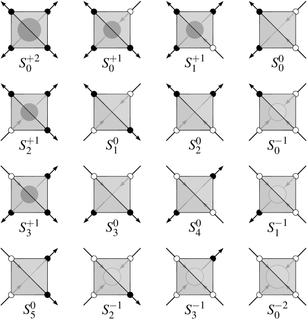
Figure 10: The sixteen states, $S^{Q}_{\mu}$, of a single tetrahedron organized by charge $Q=0,\pm 1,\pm 2$, as used in Eq. (37)

Films in the $[001]$ direction can be implemented simply using this formalism. First, consider (bulk) nearest neighbor spin ice composed of $L_{\perp}\times L_{\perp}\times L$ conventional cubic unit cells with periodic boundary conditions. The desired film geometry can then be realized by cutting the bonds that pass thorough a fixed plane with normal $\bm{\hat{z}}$, changing the remaining bonds on those cut tetrahedra to carry the orphan coupling $J_{\rm O}$. For $J_{\rm O}/J>0$ we define the weights, $\omega^{+}_{\rm O}(S^{Q}_{\mu})$, on such “orphan” tetrahedron to be

$${\omega}^{+}_{\rm O}(S^{0}_{1}) ={\omega}^{+}_{\rm O}(S^{0}_{4})=z_{\rm O}^{2},$$

$${\omega}^{+}_{\rm O}(S^{0}_{0}) ={\omega}^{+}_{\rm O}(S^{0}_{2})={\omega}^{+}_{\rm O}(S^{0}_{3})={\omega}^{+}_{\rm O}(S^{0}_{5})=1,$$

$${\omega}^{+}_{\rm O}(S^{\pm 1}_{\mu}) =z_{\rm O},$$

$${\omega}^{+}_{\rm O}(S^{\pm 2}_{\mu}) =z_{\rm O}^{2},$$ (38)

where $z_{\rm O}\equiv e^{-2\beta|J_{\rm O}|}$. Similarly, for $J_{\rm O}/J<0$ the weights, $\omega^{-}_{\rm O}(S^{Q}_{\mu})$, can be defined as

$${\omega}^{-}_{\rm O}(S^{0}_{1}) ={\omega}^{-}_{\rm O}(S^{0}_{4})=1,$$

$${\omega}^{-}_{\rm O}(S^{0}_{0}) ={\omega}^{-}_{\rm O}(S^{0}_{2})={\omega}^{-}_{\rm O}(S^{0}_{3})={\omega}^{-}_{\rm O}(S^{0}_{5})=z_{\rm O}^{2},$$

$${\omega}^{-}_{\rm O}(S^{\pm 1}_{\mu}) =z_{\rm O},$$

$${\omega}^{-}_{\rm O}(S^{\pm 2}_{\mu}) =1,$$ (39)

after a constant shift of the energy. The remaining non-orphan tetrahedra simply have the bulk weights given in Eq. (37) independent of $J_{\rm O}/J$.

Figure 11: Tetrahedron graphs for the (a) bulk and (b) orphan tetrahedra for $[001]$ spin ice films, as used in Eq. (40).

Next we define the probabilistic graph assignments that define the clusters, following the framework of Refs. [Kandel and Domany, 1991,Evertz, 2003]. To this end, we decompose a weight as

$$\omega(S^{Q}_{\mu})\equiv\sum_{G}\Delta(S^{Q}_{\mu},G)W(G),$$ (40)

where $G$ is a graph defined on a tetrahedron and the $\Delta(S^{Q}_{\mu},G)=0$ or $1$ are compatibility factors, with zero being incompatible and one being compatible. For our purposes, these graphs consist of isolated spins or possible pairings of two spins, as illustrated in Fig. 11(a). For the orphan tetrahedra, we do not include graphs that connect spins across the cut; the allowed graphs are shown in Fig. 11(b). The bulk tetrahedra and the $J_{\rm O}/J>0$ orphan tetrahedra graphs are defined to be compatible with a state if the pairs of spins joined take on opposite values while, for the $J_{\rm O}/J<0$ graphs, the two joined spins must be equal.

With these definitions, one can solve Eq. (40) to obtain the graph weights $W(G)$. As in the case of the partition function weights, we denoted the orphan tetrahedra to have graph weights as $W^{\pm}_{\rm O}(G)$. A solution for the bulk tetrahedra is given in Ref. [Otsuka, 2014] as

$$W(G^{0,0}) =z^{4},$$

$$W(G^{1,a}) =(z-z^{4})/3,$$

$$W(G^{2,a}) =(3-4z+z^{4})/6.$$ (41)

At low temperature, $T\ll J$, one has $z\rightarrow 0$ and thus only the three ”icelike” graphs ($G^{2,a}$) have non-zero assignment probability. In this limit, the algorithm (for the bulk case) reduces to a variant of the usual loop algorithm Melko et al. (2001). For the orphan tetrahedra one finds a solution

$$W^{\pm}_{\rm O}(G^{0,0}_{\rm O}) =z_{\rm O}^{2},$$

$$W^{\pm}_{\rm O}(G^{1,a}_{\rm O}) =z_{\rm O}(z_{\rm O}-1),$$

$$W^{\pm}_{\rm O}(G^{2,0}_{\rm O}) =(z_{\rm O}-1)^{2}.$$ (42)

These weights are positive and satisfy the required sum rules for any choice of $J_{\rm O}$ Otsuka (2014). At low temperature, $T\ll J_{\rm O}$, one has $z_{\rm O}\rightarrow 0$, with only the two pair graphs ($G^{2,0}_{\rm O}$) having non-zero probability. For $J_{\rm O}/J>0$ this corresponds to continuing the usual loops along the surface, while for the $J_{\rm O}/J<0$ case it corresponds to a loop where the alternation pattern is reversed when an orphan bond is encountered, as discussed in Sec. V [see Fig. 8(c)]. For $J_{\rm O}/J=0$, one has $z_{\rm O}=1$ and thus only the free graph ($G^{0,0}_{\rm O}$) has non-zero assignment probability. This corresponds to allowing the strings of alternating spins to end at the orphan bonds. Note that these probabilities factorize; we could also define the weights on the orphan bonds separately at each surface, rather than using a combined orphan tetrahedron.

The method then proceeds as usual, as discussed in Refs. [Kandel and Domany, 1991,Evertz, 2003,Otsuka, 2014]. A Monte Carlo step consists of first assigning graphs to each tetrahedron following the probabilities, $W(G)$, given in Eq. (41) and (42). When assigned to the whole lattice, these graphs form clusters, in this case strings and loops, which are identified and then flipped or not flipped with equal probability Swendsen and Wang (1987).

References

- Kogut (1979) John B. Kogut, “An introduction to lattice gauge theory and spin systems,” Rev. Mod. Phys. 51, 659–713 (1979).
- Nagaosa (1999) N. Nagaosa, Quantum Field Theory in Strongly Correlated Electronic Systems (Springer-Verlag, Berlin, Heidelberg, 1999).
- Wen (2004) X.-G. Wen, Quantum Field Theory of Many-body Systems (Oxford University Press Inc., New York, 2004).
- Lee et al. (2006) Patrick A. Lee, Naoto Nagaosa, and Xiao-Gang Wen, “Doping a mott insulator: Physics of high-temperature superconductivity,” Rev. Mod. Phys. 78, 17–85 (2006).
- Jackson (2007) John David Jackson, Classical electrodynamics (John Wiley & Sons, 2007).
- Milton (2001) Kimball A Milton, The Casimir effect: physical manifestations of zero-point energy (World Scientific, 2001).
- Bordag et al. (2001) Michael Bordag, Umar Mohideen, and Vladimir M Mostepanenko, “New developments in the casimir effect,” Phys. Rep. 353, 1–205 (2001).
- Wang and Senthil (2016) Chong Wang and T. Senthil, “Time-reversal symmetric quantum spin liquids,” Phys. Rev. X 6, 011034 (2016).
- Harris et al. (1997) M. J. Harris, S. T. Bramwell, D. F. McMorrow, T. Zeiske, and K. W. Godfrey, “Geometrical Frustration in the Ferromagnetic Pyrochlore Ho2Ti2O7,” Phys. Rev. Lett. 79, 2554–2557 (1997).
- Ramirez et al. (1999) A. P. Ramirez, A. Hayashi, R. J. Cava, R. Siddharthan, and B. S. Shastry, “Zero-point entropy in ‘spin ice’,” Nature 399, 333–335 (1999).
- Bramwell et al. (2004) S. T. Bramwell, M. J. P. Gingras, and P. C. W. Holdsworth, “Spin Ice,” in Frustrated Spin Systems, edited by H.-T. Diep (World Scientific Publishing Co, 2004) pp. 367–456.
- Gingras (2011) Michel J. P. Gingras, “Spin ice,” in Introduction to Frustrated Magnetism: Materials, Experiments, Theory, edited by Claudine Lacroix, Philippe Mendels, and Frédéric Mila (Springer Berlin Heidelberg, Berlin, Heidelberg, 2011) pp. 293–329.
- Rau and Gingras (2015) Jeffrey G. Rau and Michel J. P. Gingras, “Magnitude of quantum effects in classical spin ices,” Phys. Rev. B 92, 144417 (2015).
- Henley (2005) C. L. Henley, “Power-law spin correlations in pyrochlore antiferromagnets,” Phys. Rev. B 71, 014424 (2005).
- Henley (2010) Christopher L. Henley, “The “Coulomb Phase” in Frustrated Systems,” Annu. Rev. Condens. Matter Phys. 1, 179–210 (2010).
- Castelnovo et al. (2012) C. Castelnovo, R. Moessner, and S. L. Sondhi, “Spin Ice, Fractionalization, and Topological Order,” Annu. Rev. Condens. Matter Phys. 3, 33–55 (2012).
- Castelnovo et al. (2008) C Castelnovo, R Moessner, and S L Sondhi, “Magnetic monopoles in spin ice.” Nature 451, 42–45 (2008).
- Gingras and McClarty (2014) M J P Gingras and P A McClarty, “Quantum spin ice: a search for gapless quantum spin liquids in pyrochlore magnets,” Rep. Prog. Phys. 77, 056501 (2014).
- Algara-Siller et al. (2015) G. Algara-Siller, O. Lehtinen, F. C. Wang, R. R. Nair, U. Kaiser, H. A. Wu, A. K. Geim, and I. V. Grigorieva, “Square ice in graphene nanocapillaries,” Nature 519, 443–445 (2015).
- Bovo et al. (2014) L Bovo, X Moya, D Prabhakaran, Yeong-Ah Soh, a T Boothroyd, N D Mathur, G Aeppli, and S T Bramwell, “Restoration of the third law in spin ice thin films.” Nat. Commun. 5, 3439 (2014).
- Petrenko (2014) O. Petrenko, “Oxide heterostructures: Thin spin ice under investigation.” Nat. Mater. 13, 430–1 (2014).
- Leusink et al. (2014) D. P. Leusink, F. Coneri, M. Hoek, S. Turner, H. Idrissi, G. Van Tendeloo, and H. Hilgenkamp, “Thin films of the spin ice compound Ho2Ti2O7,” APL Materials 2, 032101 (2014).
- Note (1) We note that the results of Pomaranski et al. (2013) report a release of some of the spin ice entropy at very low temperatures in bulk Dy2Ti2O7. The origin of this release is still a matter of debate Henelius et al. (2016); Borzi et al. (2016).
- She et al. (2017) Jian-Huang She, Choong H Kim, Craig J Fennie, Michael J Lawler, and Eun-Ah Kim, “Topological superconductivity in metal/quantum-spin-ice heterostructures,” npj Quantum Materials 2, 64 (2017).
- Sasaki et al. (2014) T Sasaki, E Imai, and I Kanazawa, “Witten effect and fractional electric charge on the domain wall between topological insulators and spin ice compounds,” J. Phys. Conf. Ser. 568 (2014).
- Jaubert et al. (2017) L. D. C. Jaubert, T. Lin, T. S. Opel, P. C. W. Holdsworth, and M. J. P. Gingras, “Spin ice thin film: Surface ordering, emergent square ice, and strain effects,” Phys. Rev. Lett. 118, 207206 (2017).
- Isakov et al. (2004) S. V. Isakov, K. Gregor, R. Moessner, and S. L. Sondhi, “Dipolar spin correlations in classical pyrochlore magnets,” Phys. Rev. Lett. 93, 167204 (2004).
- Dantchev et al. (2014) D. Dantchev, J. Bergknoff, and J. Rudnick, “Casimir force in the O(n) model with free boundary conditions,” Phys. Rev. E 89, 042116 (2014).
- Rehn et al. (2017) J. Rehn, Arnab Sen, and R. Moessner, “Fractionalized classical heisenberg spin liquids,” Phys. Rev. Lett. 118, 047201 (2017).
- Anderson (1956) P. W. Anderson, “Ordering and antiferromagnetism in ferrites,” Phys. Rev. 102, 1008–1013 (1956).
- den Hertog and Gingras (2000) B C den Hertog and M J P Gingras, “Dipolar interactions and origin of spin ice in Ising pyrochlore magnets,” Phys. Rev. Lett. 84, 3430–3433 (2000).
- Isakov et al. (2005) S. V. Isakov, R. Moessner, and S. L. Sondhi, “Why spin ice obeys the ice rules,” Phys. Rev. Lett. 95, 217201 (2005).
- Gingras and den Hertog (2001) M J P Gingras and B C den Hertog, “Origin of spin-ice behavior in Ising pyrochlore magnets with long-range dipole interactions: an insight from mean-field theory,” Can. J. Phys. 79, 1339–1351 (2001).
- Zhou et al. (2008) H. D. Zhou, C. R. Wiebe, J. A. Janik, L. Balicas, Y. J. Yo, Y. Qiu, J. R. D. Copley, and J. S. Gardner, “Dynamic spin ice: Pr2Sn2O7,” Phys. Rev. Lett. 101, 227204 (2008).
- Kimura et al. (2013) Kenta Kimura, S Nakatsuji, JJ Wen, C Broholm, MB Stone, E Nishibori, and H Sawa, “Quantum fluctuations in spin-ice-like Pr2Zr2O7,” Nat. Commun. 4, 1934 (2013).
- Sibille et al. (2016) Romain Sibille, Elsa Lhotel, Monica Ciomaga Hatnean, Geetha Balakrishnan, Björn Fåk, Nicolas Gauthier, Tom Fennell, and Michel Kenzelmann, “Candidate quantum spin ice in the pyrochlore Pr2Hf2O7,” Phys. Rev. B 94, 024436 (2016).
- Onoda and Tanaka (2010) Shigeki Onoda and Yoichi Tanaka, “Quantum melting of spin ice: Emergent cooperative quadrupole and chirality,” Phys. Rev. Lett. 105, 047201 (2010).
- Onoda and Tanaka (2011) Shigeki Onoda and Yoichi Tanaka, “Quantum fluctuations in the effective pseudospin- model for magnetic pyrochlore oxides,” Phys. Rev. B 83, 094411 (2011).
- Note (2) Our convention for the orphan-bond exchange is different than that used in Ref. [\rev@citealpJaubert2016]. In the latter, an orphan bond has an exchange that differs from the bulk exchange by , with positive or negative. We thus have in the notation of Ref. [\rev@citealpJaubert2016].
- Stanley (1968) H. E. Stanley, “Spherical model as the limit of infinite spin dimensionality,” Phys. Rev. 176, 718–722 (1968).
- Bramwell et al. (1994) S T Bramwell, M J P Gingras, and J N Reimers, “Order by disorder in an anisotropic pyrochlore lattice antiferromagnet,” J. Appl. Phys. 75, 5523–5525 (1994).
- Moessner and Chalker (1998a) R. Moessner and J. T. Chalker, “Properties of a classical spin liquid: the Heisenberg pyrochlore antiferromagnet,” Phys. Rev. Lett. 80, 2929 (1998a).
- Moessner and Chalker (1998b) R. Moessner and J. T. Chalker, “Low-temperature properties of classical geometrically frustrated antiferromagnets,” Phys. Rev. B 58, 12049–12062 (1998b).
- Conlon and Chalker (2010) P. H. Conlon and J. T. Chalker, “Absent pinch points and emergent clusters: Further neighbor interactions in the pyrochlore heisenberg antiferromagnet,” Phys. Rev. B 81, 224413 (2010).
- Silverstein et al. (2014) H. J. Silverstein, K. Fritsch, F. Flicker, A. M. Hallas, J. S. Gardner, Y. Qiu, G. Ehlers, A. T. Savici, Z. Yamani, K. A. Ross, B. D. Gaulin, M. J. P. Gingras, J. A. M. Paddison, K. Foyevtsova, R. Valenti, F. Hawthorne, C. R. Wiebe, and H. D. Zhou, “Liquidlike correlations in single-crystalline Y2Mo2O7: An unconventional spin glass,” Phys. Rev. B 89, 054433 (2014).
- Sen et al. (2013) Arnab Sen, R. Moessner, and S. L. Sondhi, “Coulomb phase diagnostics as a function of temperature, interaction range, and disorder,” Phys. Rev. Lett. 110, 107202 (2013).
- Note (3) In principle, the could also depend on the sublattice index . However, we find that for the cases of interest, the symmetries of the film enforce uniformity of the constraint fields within each layer (independent of ).
- Otsuka (2014) Hiromi Otsuka, “Cluster algorithm for monte carlo simulations of spin ice,” Phys. Rev. B 90, 220406 (2014).
- Melko et al. (2001) R G Melko, B C den Hertog, and M J P Gingras, “Long-range order at low temperatures in dipolar spin ice.” Phys. Rev. Lett. 87, 067203 (2001).
- Melko and Gingras (2004) Roger G Melko and Michel JP Gingras, “Monte carlo studies of the dipolar spin ice model,” J. Phys. Condens. Matter 16, R1277 (2004).
- Swendsen and Wang (1987) Robert H. Swendsen and Jian-Sheng Wang, “Nonuniversal critical dynamics in monte carlo simulations,” Phys. Rev. Lett. 58, 86–88 (1987).
- Wolff (1989) Ulli Wolff, “Collective monte carlo updating for spin systems,” Phys. Rev. Lett. 62, 361–364 (1989).
- Castelnovo et al. (2011) C. Castelnovo, R. Moessner, and S. L. Sondhi, “Debye-hückel theory for spin ice at low temperature,” Phys. Rev. B 84, 144435 (2011).
- Note (4) For the bulk case, there is an (ad-hoc) procedure to cure this discrepancy. Specifically, as discussed in Ref. [\rev@citealpSen2013], one can simply replace the temperature dependence of the stiffness () from large- by the appropriate exponential form. This is not straightforward for films since the constraint fields, now have an explicit layer dependence. While one could define a inhomogeneous stiffness for each tetrahedron, it is ambiguous how to do this for each layer (since there are two layers per tetrahedron).
- Note (5) In the dumbbell picture, where each spin is represented by a pair of (effective) magnetic charges , these surface monopoles carry charge Jaubert et al. (2017), as they are the endpoints of two flux lines (corresponding to the two aligned orphan bond spins).
- Brooks-Bartlett et al. (2014) M. E. Brooks-Bartlett, S. T. Banks, L. D. C. Jaubert, A. Harman-Clarke, and P. C. W. Holdsworth, “Magnetic-moment fragmentation and monopole crystallization,” Phys. Rev. X 4, 011007 (2014).
- Jaubert et al. (2013) L. D. C. Jaubert, M. J. Harris, T. Fennell, R. G. Melko, S. T. Bramwell, and P. C. W. Holdsworth, “Topological-sector fluctuations and curie-law crossover in spin ice,” Phys. Rev. X 3, 011014 (2013).
- Hermele et al. (2004) Michael Hermele, Matthew P. A. Fisher, and Leon Balents, “Pyrochlore photons: The spin liquid in a three-dimensional frustrated magnet,” Phys. Rev. B 69, 064404 (2004).
- Note (6) Equivalently, these winding numbers can be directly related to the three components of the total magnetization, as discussed in Ref. [\rev@citealpJaubert2013].
- Note (7) The criterion proposed in Ref. [\rev@citealpRehn2017] for identifying a classical spin liquid in the large- theory also holds here. For films the spectrum of has a set of zero-energy flat bands. For there is no gap between these low-lying bands and the higher bands; for there is such a gap. Furthermore, the emergence of this classical spin liquid is related to structure of the dual lattice Rehn et al. (2017); when the orphan bond spins are aligned at low temperature, rendering the dual lattice non-bipartite upon identification of the two orphan bond sites.
- Motrunich (2003) O. I. Motrunich, “Bosonic model with fractionalization,” Phys. Rev. B 67, 115108 (2003).
- Rehn et al. (2016) J. Rehn, Arnab Sen, Kedar Damle, and R. Moessner, “Classical spin liquid on the maximally frustrated honeycomb lattice,” Phys. Rev. Lett. 117, 167201 (2016).
- Note (8) There is another possibility for and films: surface terminations where only one spin per surface tetrahedron remains. In that case, the appearance of surface charges is expected for any number of spin components.
- Wen et al. (2017) J.-J. Wen, S. M. Koohpayeh, K. A. Ross, B. A. Trump, T. M. McQueen, K. Kimura, S. Nakatsuji, Y. Qiu, D. M. Pajerowski, J. R. D. Copley, and C. L. Broholm, “Disordered route to the coulomb quantum spin liquid: Random transverse fields on spin ice in Pr2Zr2O7,” Phys. Rev. Lett. 118, 107206 (2017).
- Jaubert et al. (2010) L. D. C. Jaubert, J. T. Chalker, P. C. W. Holdsworth, and R. Moessner, “Spin ice under pressure: Symmetry enhancement and infinite order multicriticality,” Phys. Rev. Lett. 105, 087201 (2010).
- Wannier (1950) G. H. Wannier, “Antiferromagnetism. the triangular ising net,” Phys. Rev. 79, 357–364 (1950).
- Lee et al. (2010) Seung Hun Lee, Hidenori Takagi, Despina Louca, Masaaki Matsuda, Sungdae Ji, Hiroaki Ueda, Yutaka Ueda, Takuro Katsufuji, Jae Ho Chung, Sungil Park, Sang Wook Cheong, and Collin Broholm, “Frustrated magnetism and cooperative phase transitions in spinels,” J. Phys. Soc. Jpn. 79, 1–14 (2010).
- Krizan and Cava (2014) J. W. Krizan and R. J. Cava, “NaCaCo2F7: A single-crystal high-temperature pyrochlore antiferromagnet,” Phys. Rev. B 89, 214401 (2014).
- Krizan and Cava (2015) J. W. Krizan and R. J. Cava, “NaCaNi2F7: A frustrated high-temperature pyrochlore antiferromagnet with ,” Phys. Rev. B 92, 014406 (2015).
- Champion et al. (2003) J. D. M. Champion, M. J. Harris, P. C. W. Holdsworth, A. S. Wills, G. Balakrishnan, S. T. Bramwell, E. Čižmár, T. Fennell, J. S. Gardner, J. Lago, D. F. McMorrow, M. Orendáč, A. Orendáčová, D. McK. Paul, R. I. Smith, M. T. F. Telling, and A. Wildes, “Er2Ti2O7: Evidence of quantum order by disorder in a frustrated antiferromagnet,” Phys. Rev. B 68, 020401 (2003).
- Zhitomirsky et al. (2012) M. E. Zhitomirsky, M. V. Gvozdikova, P. C. W. Holdsworth, and R. Moessner, “Quantum order by disorder and accidental soft mode in Er2Ti2O7,” Phys. Rev. Lett. 109, 077204 (2012).
- Savary et al. (2012) Lucile Savary, Kate A. Ross, Bruce D. Gaulin, Jacob P. C. Ruff, and Leon Balents, “Order by quantum disorder in Er2Ti2O7,” Phys. Rev. Lett. 109, 167201 (2012).
- Dun et al. (2014) Z. L. Dun, M. Lee, E. S. Choi, A. M. Hallas, C. R. Wiebe, J. S. Gardner, E. Arrighi, R. S. Freitas, A. M. Arevalo-Lopez, J. P. Attfield, H. D. Zhou, and J. G. Cheng, “Chemical pressure effects on magnetism in the quantum spin liquid candidates YbO7 (Sn, Ti, Ge),” Phys. Rev. B 89, 064401 (2014).
- Dun et al. (2015) Z. L. Dun, X. Li, R. S. Freitas, E. Arrighi, C. R. Dela Cruz, M. Lee, E. S. Choi, H. B. Cao, H. J. Silverstein, C. R. Wiebe, J. G. Cheng, and H. D. Zhou, “Antiferromagnetic order in the pyrochlores Ge2O7 ( Er, Yb),” Phys. Rev. B 92, 140407 (2015).
- Hallas et al. (2016) A. M. Hallas, J. Gaudet, N. P. Butch, M. Tachibana, R. S. Freitas, G. M. Luke, C. R. Wiebe, and B. D. Gaulin, “Universal dynamic magnetism in Yb pyrochlores with disparate ground states,” Phys. Rev. B 93, 100403 (2016).
- Hallas et al. (2018) Alannah M. Hallas, Jonathan Gaudet, and Bruce D. Gaulin, “Experimental insights into ground-state selection of quantum XY pyrochlores,” Annu. Rev. Condens. Matter Phys. 9, 105–124 (2018).
- Taillefumier et al. (2017) Mathieu Taillefumier, Owen Benton, Han Yan, L. D. C. Jaubert, and Nic Shannon, “Competing spin liquids and hidden spin-nematic order in spin ice with frustrated transverse exchange,” Phys. Rev. X 7, 041057 (2017).
- Moessner and Sondhi (2003) R. Moessner and S. L. Sondhi, “Theory of the [111] magnetization plateau in spin ice,” Phys. Rev. B 68, 064411 (2003).
- Jaubert et al. (2008) L. D. C. Jaubert, J. T. Chalker, P. C. W. Holdsworth, and R. Moessner, “Three-dimensional Kasteleyn transition: Spin ice in a [100] field,” Phys. Rev. Lett. 100, 067207 (2008).
- Ruff et al. (2005) Jacob P. C. Ruff, Roger G. Melko, and Michel J. P. Gingras, “Finite-temperature transitions in dipolar spin ice in a large magnetic field,” Phys. Rev. Lett. 95, 097202 (2005).
- Polyakov (1977) Alexander M Polyakov, “Quark confinement and topology of gauge theories,” Nucl. Phys. B 120, 429–458 (1977).
- Henry and Roscilde (2014) Louis-Paul Henry and Tommaso Roscilde, “Order-by-disorder and quantum coulomb phase in quantum square ice,” Phys. Rev. Lett. 113, 027204 (2014).
- Carrasquilla et al. (2015) Juan Carrasquilla, Zhihao Hao, and Roger G Melko, “A two-dimensional spin liquid in quantum kagome ice,” Nat. Commun. 6, 7421 (2015).
- Kandel and Domany (1991) Daniel Kandel and Eytan Domany, “General cluster monte carlo dynamics,” Phys. Rev. B 43, 8539–8548 (1991).
- Evertz (2003) Hans Gerd Evertz, “The loop algorithm,” Adv. Phys. 52, 1–66 (2003).
- Pomaranski et al. (2013) D Pomaranski, LR Yaraskavitch, S Meng, KA Ross, HML Noad, HA Dabkowska, BD Gaulin, and JB Kycia, “Absence of Pauling’s residual entropy in thermally equilibrated Dy2Ti2O7,” Nat. Phys. 9, 353 (2013).
- Henelius et al. (2016) P. Henelius, T. Lin, M. Enjalran, Z. Hao, J. G. Rau, J. Altosaar, F. Flicker, T. Yavors’kii, and M. J. P. Gingras, “Refrustration and competing orders in the prototypical Dy2Ti2O7 spin ice material,” Phys. Rev. B 93, 024402 (2016).
- Borzi et al. (2016) RA Borzi, FA Gómez Albarracín, HD Rosales, GL Rossini, Alexander Steppke, D Prabhakaran, AP Mackenzie, DC Cabra, and SA Grigera, “Intermediate magnetization state and competing orders in Dy2Ti2O7 and Ho2Ti2O7,” Nat. Commun. 7, 12592 (2016).