Tensor Perturbations in Anisotropically Curved Cosmologies

Abstract

Besides expanding anisotropically, the universe can also be anisotropic at the level of its (spatial) curvature. In particular, models with anisotropic curvature and isotropic expansion leads both to a $\Lambda$CDM-like phenomenology and to an isotropic and homogeneous CMB at the background level. Thus, they offer an interesting and viable example where the cosmological principle does not follow from the isotropy of observational data. In this paper we extract the linear dynamics of tensor perturbations in two classes of cosmologies with anisotropic spatial curvature. Two difficulties arise in comparison to the same computation in isotropic cosmologies. First, the two tensor polarizations do not behave as a spin-2 field, but rather as the spin-0 and spin-1 irreducible components of a symmetric, traceless and transverse tensor field, each with its own dynamics. Second, because metric perturbations are algebraically coupled, one cannot ignore scalar and vector modes and focus just on tensors — even if one is only interested in the latter — under the penalty of obtaining the wrong equations of motion. We illustrate our results by finding analytical solutions and evaluating the power-spectra of tensor polarizations in a radiation dominated universe. We conclude with some comments on how these models could be constrained with future experiments on CMB polarization.

1 Introduction

The recent detection of gravitational waves through a binary system of black holes by the LIGO and VIRGO collaborations [1, 2, 3] is arguably a landmark in the history of science. In addition to confirming General Relativity as a full-fledged theory of gravitational interactions, it represents the birth of a new observational era to physicists and astronomers, from which unfathomable new features of the universe might arise.

From the perspective of cosmology, the detection of gravitational waves from astrophysical processes renews our hope that primordial gravitational waves might also be detected in the coming future. Such discovery would have a huge impact to cosmology, since primordial gravitational waves are believed to be the fingerprint of an early (and yet not fully understood) inflationary stage of the universe. While the path leading to this discovery is still being worked upon, there are a number of cosmological phenomena closely linked to the physics of primordial gravitational waves that can help us to indirectly measure them. For instance, the dynamics of primordial gravitational waves is supposed to leave an imprint both in the temperature spectrum of the Cosmic Microwave Background (CMB) radiation — which was measured with exquisite accuracy by WMAP [4] and Planck [5] collaborations — and in the polarization spectrum of $B$-modes of CMB, which is the main goal of current and future CMB missions [6, 7, 8]. For this reason, it is an important task to investigate the dynamics of gravitational waves under given cosmological hypotheses and compare them with cosmological data.

Indeed, one of the central hypothesis believed to be backed up by data like galaxy distribution from the Sloan Digital Sky Survey [9] and CMB temperature fluctuations by the Planck satellite [10], is that around 100 Mpc and above, the average spatial distribution of matter in the universe is isotropic. Such spherical symmetry around us together with the Copernican principle — according to which our position in the universe is not special — constitutes a hallmark of modern cosmology known as the Cosmological Principle. Based on this principle, cosmology has had an incredible advance in the last decades, from both theoretical and observational points of view, culminating in a very successful concordance cosmological model, the $\Lambda$CDM model.

Although very successful in describing the large-scale structure of the universe — even though several problems still persist [11] — one should not lose sight of the fact that the $\Lambda$CDM depends on untested assumptions about the symmetries of matter distribution at cosmological scales. Thus, such assumptions should not prevent us from considering alternative cosmological models which are compatible with the data. In fact, in the past few years several authors have considered the possibility of giving up the Cosmological Principle in a way or another. Some examples of these are large void models which attempt to fit the spectrum of CMB assuming that we would be located near the center of a spherically symmetrical universe [12, 13, 14, 15], and spatially homogeneous but anisotropic cosmological models which are justified either as an explanation for the statistical anomalies of the CMB [16, 17, 18, 19] or as a mean of constraining the impact of spatial anisotropy on CMB data [20, 21, 22, 23]. The interest in inhomogeneous and anisotropic models has in fact a richer history prior to modern CMB data — see for example [24, 25, 26, 27, 28].

Here we contribute to this task by investigating a class of homogeneous but spatially anisotropic models such that their time-constant hypersurfaces have a preferred direction, but which nonetheless preserve the observed isotropy of CMB at first order (i.e., without including perturbations). This is possible because the anisotropy of these spacetimes results from the curvature of the spatial sections, and not from the kinematics of expansion [29, 30]. From a fundamental perspective, such as in string inspired models of the early universe, one can argue that the early universe’s dimensions were initially small and compact [31]. In this scenario, it is plausible that a process of decompactification of our three spatial dimensions acts anisotropically (via, e.g., anisotropic bubble nucleation [32]), producing a universe with different topologies along different spatial dimensions [33, 34].

Specifically, we focus on two particular solutions of Einsteins equations with these properties, namely, Bianchi type III (BIII) and Kantowski-Sachs (KS) metrics. In 1993, Mimoso and Crawford [35] showed that these metrics admit a geodesic, irrotational and isotropic (or shear-free) expansion provided that the anisotropic stress-tensor of the cosmological budget is in direct proportion to the electric part of the Weyl tensor. The interplay between the energy-momentum tensor and the shear-free condition was further explored in [36, 37]. An analogous result was also found by Carneiro and Marugán [38, 39] who deployed a clever use of an anisotropic scalar field to balance the anisotropy of the spatial curvature. Under this condition the scale factor has the same dynamics of a spatially curved Friedmann-Lemaître-Robertson-Walker (FLRW) universe and the metric can be brought to a conformally static form. It then follows that the electromagnetic radiation, e.g. CMB, will be isotropic, in accordance with basic observations [40, 41], even though the geometry is fundamentally anisotropic. Thus, these models offer an important lesson: contrarily to common belief, the symmetries of cosmological data do not necessarily imply the symmetries of the cosmic geometry [36].

The background phenomenology of BIII and KS shear-free cosmologies was originally explored in refs. [35, 38]. In [42], the impact of a directional spatial curvature on the distribution of type Ia supernovae was also investigated. The linear and gauge-invariant perturbation theory in such models was also shown to be viable in [29], and in several ways parallels that of standard perturbation theory in FLRW spacetimes, though the expected observational signatures are of course different [30]. In this work, motivated by the recent detection of gravitational waves, we focus on the linear dynamics of tensor perturbations in these models. We thus begin §2 by briefly reviewing the geometrical and dynamical aspects of geometries with anisotropic curvature. Since our goal is to find the dynamics of tensor perturbations in spacetimes with, as we shall see, a residual rotational symmetry, and then later contrast our results with tensor perturbations in FLRW spacetimes, we present in §3 a systematic description of the irreducible decomposition of symmetric tensors in the 1+3 and 1+2+1 spacetime splittings, together with a dictionary to go from one to the other. These steps will allow us to pinpoint the genuine gauge-invariant tensor degrees of freedom in a spacetime with anisotropic curvature in §4. Next, we use linear perturbation theory to find the equations of motion of the tensorial degrees of freedom in §5, after which we present some simple applications. As we shall see, and differently from what happens with perturbation theory in FLRW spacetimes, this task requires that we keep track of all metric degrees of freedom — including those not related to gravitational waves — since algebraic couplings between different modes cannot be ignored, under penalty of leading to the wrong dynamics of gravitational waves. We finally conclude and give some perspectives of further developments in §6.

Throughout this work, dots will represent derivatives along time, whereas a prime is reserved for derivatives along the anisotropic spatial direction. We also adopt units such that $c=1=8\pi G$, and spacetime signature $\left(-,+,+,+\right)$.

2 Background model

In this work we are interested in a class of homogeneous and conformally static geometries codified by the following line element:

$${\rm d}s^{2} =a^{2}(\eta)\left[-{\rm d}\eta^{2}+\gamma_{ij}\left(\mathbf{x}\right){\rm d}x^{i}{\rm d}x^{j}\right],$$ (2.1)

where $\eta$ is the usual conformal time parameter and $\gamma_{ij}(\mathbf{x})$ is the spatial metric. Because $\partial_{\eta}\gamma_{ij}(\mathbf{x})=0$, these models have no geometrical shear, and the expansion is isotropic. However, we can still have spatial anisotropies if $\gamma_{ij}$ describes manifolds whose (spatial) curvature is direction-dependent. Since one-dimensional manifolds are trivially flat, the simplest examples one can think of (i.e., without invoking non-trivial topologies) are given by metrics on spaces of the form ${\cal M}^{2}\times\mathbb{R}$, where ${\cal M}^{2}$ is a two-dimensional maximally symmetric space. Adopting a coordinate system where the real line coincides with the $z$-axis, we have

$$\gamma_{ij}{\rm d}x^{i}{\rm d}x^{j}=\mathcal{S}_{ab}(x^{c}){\rm d}x^{a}{\rm d}x^{b}+{\rm d}z^{2}\,,$$ (2.2)

where $\{a,b,c\}$ run from 1 to 2 and ${\cal S}_{ab}$ is the metric on ${\cal M}^{2}$. Because of the residual symmetry of these spaces, it is convenient to employ cylindrical coordinates so that

$${\rm d}s^{2}=a^{2}(\eta)\left[-{\rm d}\eta^{2}+{\rm d}\rho^{2}+S_{\kappa}^{2}(\rho){\rm d}\varphi^{2}+{\rm d}z^{2}\right]\,,$$ (2.3)

where the function $S_{\kappa}(\rho)$ is defined as

$$S_{\kappa}(\rho)=\frac{1}{\sqrt{\kappa}}\sin(\sqrt{\kappa}\rho)\,.$$ (2.4)

Note that, for $\kappa<0$, this parameterization gives $S_{\kappa}=\sinh(\sqrt{|\kappa|}\rho)/\sqrt{|\kappa|}\rho$, as it should. We adopt a convention where the scale factor is dimensionless and comoving coordinates have dimension of length. Thus, the curvature parameter $\kappa$ has units of $({\rm length})^{-2}$, being either negative, positive or zero. Topologically, this means that ${\cal M}^{2}$ corresponds to either the pseudo-sphere $\mathbb{H}^{2}$ ($\kappa<0$), the two-sphere $\mathbb{S}^{2}$ $(\kappa>0)$ or the plane $\mathbb{R}^{2}$ ($\kappa=0$). In cosmology, this leads to the solutions of Bianchi type-III (BIII), Kantowski-Sachs (KS) and flat Friedmann-Lemaître-Robertson-Walker (FLRW) universes, respectively. The flat case is included only for consistency, since it allows us to verify the validity of our results in the limit $|\kappa|\ll 1$. Thus, in what follows we treat $\kappa$ as a free parameter.

2.1 Shear-free dynamics

The family of spacetimes described by (2.3) are usually known as spacetimes with anisotropic curvature, or shear-free spacetimes. These adjectives stem from the already mentioned fact that the spacetime expansion is isotropic even though the metric is genuinely anisotropic. But since anisotropic models cannot simultaneously exhibit shear-free expansion and a perfect fluid matter content [35], shear-free models can only be realized at the expense of an imperfect energy-momentum tensor of the form

$$T_{\mu\nu}=(\rho+p)u_{\mu}u_{\nu}+pg_{\mu\nu}+\pi_{\mu\nu}\,,$$ (2.5)

with the condition $u^{\mu}\pi_{\mu\nu}=0=\pi_{\phantom{\mu}\mu}^{\mu}$. In the coordinate system (2.3), Einstein background equations are

$$\frac{3\mathcal{H}^{2}}{a^{2}}+\frac{\kappa}{a^{2}} =\rho_{f}+\rho\,,$$

$$\frac{{\cal H}^{2}}{a^{2}}+2\frac{\dot{{\cal H}}}{a^{2}} =-p_{f}-p-\pi_{\phantom{\mu}1}^{1}\,,$$

$$\frac{{\cal H}^{2}}{a^{2}}+2\frac{\dot{{\cal H}}}{a^{2}}+\frac{\kappa}{a^{2}} =-p_{f}-p-\pi_{\phantom{\mu}3}^{3}\,,$$

where $\rho_{f}$ and $p_{f}$ are the total energy density and pressure of additional perfect fluids. Note that the residual symmetry of the metric implies that $\pi_{\phantom{\mu}1}^{1}=\pi_{\phantom{\mu}2}^{2}$, while the trace-free condition on $\pi_{\mu\nu}$ gives $\pi_{\phantom{\mu}3}^{3}=-2\pi_{\phantom{\mu}1}^{1}$. Consistency between the last two equations further requires that

$$\pi_{\phantom{\mu}1}^{1}=\frac{\kappa}{3a^{2}}\,.$$ (2.6)

This is known as the shear-free condition, and it follows from our imposition of metric (2.3) as a solution of Einstein equations. From the phenomenological point of view, the simplest model implementing (2.6) is perhaps that of a massless scalar field with Lagrangian

$${\cal L}_{\phi}=-\frac{\alpha}{2}\partial_{\mu}\phi\partial^{\mu}\phi\,,$$ (2.7)

where $\alpha$ is a constant. Written in the form (2.5), the energy-momentum tensor of the field $\phi$ gives

$$\rho=\frac{\alpha}{2}\partial_{\lambda}\phi\partial^{\lambda}\phi\,,\quad p=-\frac{1}{3}\rho\,,\quad\pi_{\phantom{\mu}\nu}^{\mu}=\alpha\partial^{\mu}\phi\partial_{\nu}\phi-\frac{2}{3}\left(\delta_{\nu}^{\mu}+u^{\mu}u_{\nu}\right)\rho\,.$$ (2.8)

The condition $u_{\mu}\pi_{\phantom{\mu}\nu}^{\mu}=0$ implies that $\partial_{\eta}\phi=0$, which tell us that $\phi$ has no dynamics. It is easy to verify that $\phi=z$ satisfies this condition as well as the wave equation $\square\phi=0$ [38]. This implies that

$$\pi_{\phantom{\mu}1}^{1}=-\frac{2}{3}\rho=2p=-\frac{\alpha}{3a^{2}}\,,$$ (2.9)

which, when compared to (2.6), gives $\alpha=-\kappa$. Note that, while $\phi$ is inhomogeneous, its energy density, pressure and stress are not, so that the homogeneity of the background is preserved. Such field could arise, for example, in a field-theoretic description of a solid inflating the universe [43, 44]. The phenomenology leading to (2.6) can also be obtained with a three-form (Kalb-Ramon) field [42] and, in general, shear-free solutions can be obtained with $p$-form gauge fields [45]. Luckily for us, the precise form of the field leading to a shear-free expansion will not affect the dynamics of tensor perturbations, as we will see. The effective background equations then become

$$\begin{split}{\cal H}^{2}&=\frac{\rho_{f}a^{2}}{3}-\frac{\kappa}{2}\,,\\ \frac{\ddot{a}}{a}&=\frac{1}{6}(\rho_{f}-3p_{f})a^{2}-\frac{\kappa}{2}\,.\end{split}$$ (2.10)

Although not written in a standard from, these are essentially Friedmann equations in a background with curvature $\kappa/2$ (see, e.g., [46]). Since $\kappa$ is a free parameter, it is convenient to introduce a curvature radius $R_{c}$ through

$$\left|\kappa\right|\equiv\frac{1}{R_{c}^{2}}=2H_{0}^{2}\left|\Omega_{\kappa 0}\right|=\frac{2}{L_{c}^{2}}\,,$$ (2.11)

where $H_{0}$ is today’s Hubble parameter in physical time and $L_{c}=H_{0}^{-1}\left|\Omega_{\kappa 0}\right|^{-1/2}$ is the curvature radius of FLRW metrics.

3 Spacetime splittings

Our main goal is to derive the dynamics of tensor perturbations evolving in the metric (2.3), with the background evolution being given by (2.10). However, because the background space is not maximally symmetric, the very definition of tensor perturbations needs to be revisited. We thus start this section by briefly recalling the definitions and properties of the 1+3 spacetime splitting, followed by a review of its less notorious cousin, the 1+2+1 splitting. Such splittings will be combined with (versions of) the Scalar-Vector-Tensor (SVT) decomposition in the next section to arrive at a proper definition of gravitational waves in spacetimes with anisotropic spatial curvature. We stress that our goal is not to conduct a fully covariant characterization of gravitational wave dynamics — to which treatment we point the reader to refs. [47, 48, 49, 50, 51]. Rather, we use a covariant approach only to identify the “pure” tensor modes in spacetimes with anisotropic curvature, after which we will adopt a more direct coordinate-based approach to find the dynamics of gravitational waves.

Since the introduction of a new algebraic splitting brings with it a zoo of new objects, each of which requires a special symbol, it is important to introduce a notation that avoids the proliferation of overbars, tildes and the like. Thus, we adopt the convention where spacetime (i.e., non-projected) tensors will be represented by lower case (Latin or Greek) letters; e.g, $a^{\mu}$, $g_{\mu\nu}$ and so on are spacetime quantities. In any 1+3 irreducible decomposition, each term will be represented by a capital Latin letter. Thus, objects like $V_{\mu}$, $T_{\mu\nu}$ and so on are by definition orthogonal to the observer’s four velocity $u^{\mu}$, whereas $A$, $B$ and so on denote scalars “along” $u^{\mu}$. Likewise, in any 1+2+1 irreducible decomposition, each term will be represented by calligraphic capital Latin letter. Hence, terms like ${\cal V}_{\mu}$, ${\cal T}_{\mu\nu}$, and so on are orthogonal to both $u^{\mu}$ and $N^{\mu}$ (the curvature privileged direction); likewise, ${\cal A}$, ${\cal B}$ and so on are scalars “along” either $u^{\mu}$ or $N^{\mu}$. The only exception to this rule is the fully-projected spatial metric $\gamma_{\mu\nu}$, which we keep as it is to convey to the standard literature. Moreover, we shall refer to vectors like $a_{\mu}$, $V_{\mu}$, and ${\cal V}_{\mu}$ as 4-, 3- and 2-vector, respectively. Occasionally, we shall also refer (somewhat misleadingly but hopefully useful) to tensors like $g_{\mu\nu}$, $T_{\mu\nu}$ and ${\cal T}_{\mu\nu}$ as 4-, 3- and 2-tensor, respectively.

3.1 1+3 spacetime splitting

In FLRW cosmologies with perfect-fluid matter content, the geodesic flow of matter naturally defines a congruence of timelike curves $x^{\mu}\left(\tau\right)$ such that freely falling observers with proper time $\tau$ are fully characterized by their four-velocity vector $u^{\mu}=dx^{\mu}/d\tau$, normalized so that $u^{\mu}u_{\mu}=-1$. Such field of vectors naturally define two projection tensors

$$t_{\phantom{\mu}\nu}^{\mu}\equiv-u^{\mu}u_{\nu}\,,\qquad\gamma_{\phantom{\mu}\nu}^{\mu}\equiv\delta_{\nu}^{\mu}+u^{\mu}u_{\nu}\,,$$ (3.1)

where all indices are manipulated with $g_{\mu\nu}$. It is easy to check that $t_{\mu\nu}$ projects any tensor into the time direction, whereas $\gamma_{\mu\nu}$ projects any tensor in the subspace orthogonal to $u^{\mu}$. Moreover, one has

$$t_{\phantom{\mu}\lambda}^{\mu}t_{\phantom{\mu}\nu}^{\lambda}=t_{\phantom{\mu}\nu}^{\mu}\,,\quad t_{\phantom{\mu}\mu}^{\mu}=1,\quad\gamma_{\phantom{\mu}\lambda}^{\mu}\gamma_{\phantom{\mu}\nu}^{\lambda}=\gamma_{\phantom{\mu}\nu}^{\mu}\,,\quad\gamma_{\phantom{\mu}\mu}^{\mu}=3\,,\qquad u^{\mu}\gamma_{\mu\nu}=0\,.$$ (3.2)

Quite generally, the tensor $\gamma_{\mu\nu}$ acts as the metric of local rest frames, since any two 3-vectors $A^{\mu}$ and $B^{\mu}$ will have a scalar product given by $g_{\mu\nu}A^{\mu}B^{\nu}=\gamma_{\mu\nu}A^{\mu}B^{\nu}$. However, we are interested in the case where $u^{\mu}$ is everywhere orthogonal to the spatial hypersurfaces, which further implies that $\gamma_{\mu\nu}$ is the metric on these hypersurfaces (here called $\Sigma_{\tau}$ – see figure 1).

Given the above projectors, any 4-vector $v^{\mu}$ can be covariantly decomposed into one scalar degree of freedom (d.o.f) in the time direction plus a 3-vector orthogonal to it:

$$v^{\mu}=-Vu^{\mu}+V^{\mu}\,,\qquad u_{\mu}V^{\mu}=0\,,$$ (3.3)

where $V\equiv u_{\mu}v^{\mu}$ and $V^{\mu}\equiv\gamma_{\phantom{\mu}\nu}^{\mu}v^{\nu}$. Likewise, any (symmetric) rank-two tensor $h_{\mu\nu}$ can be uniquely decomposed into two scalars $A$ and $B$ (1 d.o.f each), one 3-vector $C_{\mu}$ (3 d.o.f) and one traceless 3-tensor $H_{\mu\nu}$ (5 d.o.f) as

$$h_{\mu\nu}=2Au_{\mu}u_{\nu}+B\gamma_{\mu\nu}+2C_{(\mu}u_{\nu)}+H_{\mu\nu}$$ (3.4)

where, by definition

$$u^{\mu}C_{\mu}=0=u^{\mu}H_{\mu\nu}\,,\qquad\gamma^{\mu\nu}H_{\mu\nu}=0\,.$$ (3.5)

In terms of its irreducible components, then, the 10 d.o.f of $h_{\mu\nu}$ are split as 1+1+3+5 components in the 1+3 splitting. Conversely, scalars, 3-vectors and trace-free 3-tensors can be extracted from $h_{\mu\nu}$ in the following manner

$$\begin{aligned} A&=u^{\alpha}u^{\beta}h_{\alpha\beta}/2\,,\qquad\\ B&=\gamma^{\alpha\beta}h_{\alpha\beta}/3\,,\end{aligned} \begin{aligned} C_{\mu}&=-u^{\alpha}\gamma_{\mu}^{\phantom{\mu}\beta}h_{\alpha\beta}\,,\\ H_{\mu\nu}&=\left(\gamma_{\mu}^{\phantom{\mu}\alpha}\gamma_{\nu}^{\phantom{\mu}\beta}-\frac{1}{3}\gamma_{\mu\nu}\gamma^{\alpha\beta}\right)h_{\alpha\beta}\equiv h_{\left\langle\alpha\beta\right\rangle}\,\end{aligned}$$ (3.6)

Note that these equations implicitly define mode-extraction operators which can be applied to $h_{\mu\nu}$ to obtain a specific mode. In particular, the last equations defines the projection operator

$$P_{\mu\phantom{\mu}\nu}^{\phantom{\mu}\alpha\phantom{\mu}\beta}\equiv\left(\gamma_{\mu}^{\phantom{\mu}\alpha}\gamma_{\nu}^{\phantom{\mu}\beta}-\frac{1}{3}\gamma_{\mu\nu}\gamma^{\alpha\beta}\right)\,,$$ (3.7)

which extracts the traceless tensor component of $h_{\mu\nu}$. This operator will be crucial to obtain the propagating degrees of freedom of gravitational waves in the following section.

3.1.1 Kinematics

The existence of the projectors (3.1) allows us to define two important tensorial derivatives of tensor fields:

$$\dot{q}_{\phantom{\mu}\nu_{1}\cdots}^{\mu_{1}\cdots}\equiv u^{\lambda}\nabla_{\lambda}q_{\phantom{\mu}\nu_{1}\cdots}^{\mu_{1}\cdots}\,,\quad\text{and}\quad D_{\rho}q_{\phantom{\mu}\nu_{1}\cdots}^{\mu_{1}\cdots}\equiv\gamma_{\rho}^{\phantom{\mu}\lambda}\gamma_{\phantom{\mu}\alpha_{1}}^{\mu_{1}}\cdots\gamma_{\nu_{1}}^{\phantom{\mu}\beta_{1}}\cdots\nabla_{\lambda}q_{\phantom{\mu}\beta_{1}\cdots}^{\alpha_{1}\cdots}\,,$$ (3.8)

where $q_{\phantom{\mu}\nu_{1}\cdots}^{\mu_{1}\cdots}$ is an arbitrary spacetime tensor. These derivatives measure variations along and orthogonally to $u^{\mu}$, respectively. Note in particular that, for any scalar field $\varphi$, one has $\nabla_{\mu}\varphi=-u_{\mu}\dot{\varphi}+D_{\mu}\varphi$.

A central kinematical quantity in the 1+3 splitting is the covariant derivative of the fundamental observer’s four velocity:

$$\nabla_{\mu}u_{\nu}\equiv-u_{\mu}A_{\nu}+K_{\mu\nu}\,,$$ (3.9)

where $A_{\mu}\equiv\dot{u}_{\mu}$ is the observer’s acceleration and $K_{\mu\nu}\equiv D_{\mu}u_{\nu}$ is the extrinsic curvature of spatial hypersurfaces. The latter measures spatial deformations of timelike curves, which can be divided into an expansion ($K_{\phantom{\mu}\mu}^{\mu}$), shear ($K_{\left\langle\mu\nu\right\rangle}$) and vorticity ($K_{[\mu\nu]}$) of the congruence. Here we are interested in geodesic observers in shear-free and irrotational universes, so that from now on we set

$$A_{\mu}=K_{\left\langle\mu\nu\right\rangle}=K_{[\mu\nu]}=0\,.$$ (3.10)

In other words, $K_{\mu\nu}$ is a pure trace in the models we are considering, measuring only the expansion of timelike congruences:

$$K_{\mu\nu}\equiv\frac{\Theta}{3}\gamma_{\mu\nu}$$ (3.11)

where $\Theta$ is a scalar measuring the global expansion of geodesics. This reflects the fact that, from a kinematical point of view, shear-free universes behave exactly like FLRW ones [38]. Finally, we give for future reference two important relations that one can easily check:

$$\dot{\gamma}_{\mu\nu}=0=D_{\alpha}\gamma_{\mu\nu}\,.$$ (3.12)

3.2 1+2+1 spacetime splitting

The 1+3 spacetime splitting is quite general since it does not depend on the specific symmetries of the constant time hypersurfaces $\Sigma_{\tau}$ (left panel of figure 1). However, if $\Sigma_{\tau}$ has a privileged spacelike direction, which is the case of LRS (locally rotationally symmetric) spacetimes with anisotropic curvature, then we can covariantly split $\gamma_{\mu\nu}$ into components along and orthogonal to this direction. Let $N^{\mu}$ be a unit spacelike vector defining this direction. Such vector naturally defines two projection tensors on $\Sigma_{\tau}$:

$$N_{\phantom{\mu}\nu}^{\mu}\equiv N^{\mu}N_{\nu}\,,\quad\text{and}\quad\mathcal{S}_{\phantom{\mu}\nu}^{\mu}\equiv\gamma_{\phantom{\mu}\nu}^{\mu}-N^{\mu}N_{\nu}\,,$$ (3.13)

where $N_{\phantom{\mu}\nu}^{\mu}$ projects any tensor into the preferred spatial direction and $\mathcal{S}_{\phantom{\mu}\nu}^{\mu}$ projects any tensor orthogonally to it. From the above definitions it is easy to see that

$$N_{\phantom{\mu}\lambda}^{\mu}N_{\phantom{\mu}\nu}^{\lambda}=N_{\phantom{\mu}\nu}^{\mu}\,,\quad N_{\phantom{\mu}\mu}^{\mu}=1,\quad\mathcal{S}_{\phantom{\mu}\lambda}^{\mu}\mathcal{S}_{\phantom{\mu}\nu}^{\lambda}=\mathcal{S}_{\phantom{\mu}\nu}^{\mu}\,,\quad\mathcal{S}_{\phantom{\mu}\mu}^{\mu}=2\,,\qquad\mathcal{S}_{\phantom{\mu}\nu}^{\mu}N^{\nu}=0\,.$$ (3.14)

Being spatial projectors, they also satisfy

$$N_{\phantom{\mu}\nu}^{\mu}u^{\nu}=0=\mathcal{S}_{\phantom{\mu}\nu}^{\mu}u^{\nu}\,.$$ (3.15)

In the particular case we are interested, where $\Sigma_{\tau}={\cal M}^{2}\times\mathbb{R}$, $\mathcal{S}_{\mu\nu}$ defines the metric on the two-dimensional subspace ${\cal M}^{2}$ and is everywhere orthogonal to $N^{\mu}$ — see the right panel on figure 1.

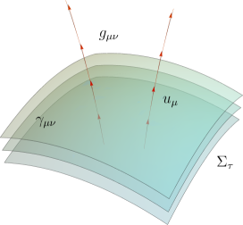
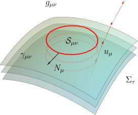
Figure 1: Schematic comparison between the 1+3 (left) and 1+2+1 (right) splittings. $\Sigma_{\tau}$ labels the three-dimensional constant-time hypersurfaces. The two-dimensional sheet ${\cal M}^{2}$ with metric $\mathcal{S}_{\mu\nu}$ is represented on the right panel by a closed (red) curve.

Given the vectors $u^{\mu}$ and $N^{\mu}$, and the metric $\mathcal{S}_{\mu\nu}$, we would like to carry an irreducible decomposition of general tensors in terms of scalars, 2-vectors, and traceless 2-tensors, where the tracefree condition is now defined with respect to $\mathcal{S}_{\mu\nu}$. We start by noting that any four-vector $v^{\mu}$ can be uniquely written in terms of two scalars and one 2-vector as

$$v^{\mu}=-Vu^{\mu}+\mathcal{U}N^{\mu}+\mathcal{V}^{\mu}\,,\qquad N_{\mu}\mathcal{V}^{\mu}=u_{\mu}\mathcal{V}^{\mu}=0\,,$$ (3.16)

where $V\equiv u_{\mu}v^{\mu}$, $\mathcal{U}\equiv N_{\mu}v^{\mu}$ and $\mathcal{V}^{\mu}\equiv\mathcal{S}_{\phantom{\mu}\nu}^{\mu}v^{\nu}$. A straightforward comparison with (3.3) reveals that $V^{\mu}=\gamma_{\phantom{\mu}\nu}^{\mu}v^{\nu}=\left(\mathcal{S}_{\phantom{\mu}\nu}^{\mu}+N^{\mu}N_{\nu}\right)v^{\nu}=\mathcal{V}^{\mu}+\mathcal{U}N^{\mu}$, as it should be, since the new splitting only affects spatially-projected quantities.

Moving forward, we can split any symmetric and rank-two tensor uniquely as

$$h_{\mu\nu}=2{\cal A}u_{\mu}u_{\nu}+{\cal B}\mathcal{S}_{\mu\nu}+2{\cal C}N_{\mu}N_{\nu}+2{\cal Q}N_{(\mu}u_{\nu)}+2\mathcal{E}_{(\mu}u_{\nu)}+2\mathcal{F}_{(\mu}N_{\nu)}+\mathcal{G}_{\mu\nu}$$ (3.17)

where, by force of our notation

$$u^{\mu}\mathcal{E}_{\mu}=N^{\mu}\mathcal{E}_{\mu}=u^{\mu}\mathcal{F}_{\mu}=N^{\mu}\mathcal{F}_{\mu}=0\,,\quad\text{and}\quad u^{\mu}\mathcal{G}_{\mu\nu}=N^{\mu}\mathcal{G}_{\mu\nu}=0=\mathcal{S}^{\mu\nu}\mathcal{G}_{\mu\nu}\,.$$ (3.18)

Looking to the right hand side of (3.18) we would be tempted to conclude that $\mathcal{G}_{\mu\nu}$ has only one independent d.o.f. However this conclusion is false since the condition $N^{\mu}\mathcal{G}_{\mu\nu}=0$ eliminates only three-variables once $u^{\mu}\mathcal{G}_{\mu\nu}=0$ is implemented. Thus we conclude that $h_{\mu\nu}$ splits as $1+1+1+1+2+2+2$ irreducible pieces in the 1+2+1 splitting. Contrarily, given $h_{\mu\nu},$ these irreducible components can be extracted as follows

$$\begin{aligned} \mathcal{E}_{\mu}&=-u^{\alpha}\mathcal{S}_{\mu}^{\phantom{\mu}\beta}h_{\alpha\beta}\,,\qquad\\ \mathcal{F}_{\mu}&=N^{\alpha}\mathcal{S}_{\mu}^{\phantom{\mu}\beta}h_{\alpha\beta}\,,\\ \mathcal{G}_{\mu\nu}&=\left(\mathcal{S}_{\mu}^{\phantom{\mu}\alpha}\mathcal{S}_{\nu}^{\phantom{\mu}\beta}-\frac{1}{2}\mathcal{S}_{\mu\nu}\mathcal{S}^{\alpha\beta}\right)h_{\alpha\beta}\equiv h_{\{\alpha\beta\}}\,.\\ \\ \end{aligned}$$ (3.19)

3.2.1 Kinematics

The introduction of the projectors $N^{\mu}$ and $\mathcal{S}_{\mu\nu}$ allow us to define two new projected derivatives [50]:

$$q_{\phantom{\mu}\,\nu_{1}\cdots}^{\,\prime\mu_{1}\cdots}\equiv N^{\lambda}D_{\lambda}q_{\phantom{\mu}\nu_{1}\cdots}^{\mu_{1}\cdots},\quad{\cal D}_{\rho}q_{\phantom{\mu}\nu_{1}\cdots}^{\mu_{1}\cdots}\equiv\mathcal{S}_{\rho}^{\phantom{\mu}\lambda}\mathcal{S}_{\phantom{\mu}\alpha_{1}}^{\mu_{1}}\cdots\mathcal{S}_{\nu_{1}}^{\phantom{\mu}\beta_{1}}\cdots D_{\lambda}q_{\phantom{\mu}\beta_{1}\cdots}^{\alpha_{1}\cdots}\,,$$ (3.20)

where $q_{\phantom{\mu}\nu_{1}\cdots}^{\mu_{1}\cdots}$ is an arbitrary spacetime tensor. It is important to note that these definitions are made with respect to the spatially projected operator $D_{\mu}$, and not to the full spacetime derivative $\mathbf{\nabla}_{\mu}$. Since $\mathcal{S}_{\mu\alpha}\gamma_{\phantom{\mu}\nu}^{\alpha}=\mathcal{S}_{\mu\nu}$, this has no effect on the definition of the operator ${\cal D}_{\mu}$. However, it does change the definition of the derivative along $N^{\mu}$ (here represented by a prime) since, for any spatial 3-vector $V_{\mu}$, one has

$$V^{\prime}_{\mu} =N^{\lambda}D_{\lambda}V_{\mu}$$

$$=N^{\lambda}\left(\gamma_{\lambda}^{\phantom{\mu}\alpha}\gamma_{\mu}^{\phantom{\mu}\beta}\nabla_{\alpha}V_{\beta}\right)$$

$$=N^{\alpha}\nabla_{\alpha}V_{\mu}+u_{\mu}u^{\beta}\left(N^{\alpha}\nabla_{\alpha}V_{\beta}\right)\,.$$

In other words, this definition ensures that $u^{\mu}V^{\prime}_{\mu}=0$, as one can easily check.

In analogy to (3.9), it will also be necessary to find the irreducible decomposition of the projected tensor $D_{\mu}N_{\nu}$. This is given by

$$D_{\mu}N_{\nu}=N_{\mu}{\cal A}_{\nu}+{\cal K}_{\mu\nu}\,,$$ (3.21)

where $\mathcal{A}_{\nu}\equiv N^{\prime}_{\nu}$ measures the observer’s acceleration along $N_{\nu}$, and $\mathcal{K}_{\mu\nu}\equiv\mathcal{D}_{\mu}N_{\nu}$ is the extrinsic curvature of ${\cal M}^{2}$. In analogy to $K_{\mu\nu}$, it measures deformations of a congruence of curves along the privileged direction. As before, such deformations can be separated into an expansion ($\mathcal{K}_{\phantom{\mu}\mu}^{\mu}$), a shear ($\mathcal{K}_{\{\mu\nu\}}$) and a torsion ($\mathcal{K}_{[\mu\nu]}$) of the bundle. However, it is important to stress that the quantities defined by $\mathcal{K}_{\mu\nu}$ are not in the exact same footing as those defined by $K_{\mu\nu}$, since the former define deformations of spacelike curves on the same surface $\Sigma_{\tau}$, whereas the latter defines deformation as time evolves, thus connecting $\Sigma_{\tau}$ to $\Sigma_{\tau+{\rm d}\tau}$. Moreover, we stress that the torsion term $\mathcal{K}_{[\mu\nu]}$ is identically zero by virtue of our choice of ${\cal S}_{\mu\nu}$ as the global metric on ${\cal M}^{2}$ (i.e., Frobenius theorem). Furthermore, since BIII and KS spacetimes are spatially homogeneous, we must have

$$\mathcal{K}_{\phantom{\mu}\mu}^{\mu}=0=\mathcal{K}_{\{\mu\nu\}}\,.$$ (3.22)

For the same reason, we should not experience any acceleration as we travel along $N^{\mu}$, for this would imply a preferred position in space. Thus we set

$${\cal A}_{\mu}=0\,.$$ (3.23)

Clearly, this conclusion would not be the same if we were working, for example, in a Schwarzschild spacetime, where radial accelerations do appear [50]. In conclusion, then, we have that

$$D_{\mu}N_{\nu}=0$$ (3.24)

for the BIII and KS models. Note however that this does not imply that $\nabla_{\mu}N_{\nu}$ is zero. Indeed we have

$$\nabla_{\mu}N_{\nu}=u_{\nu}N^{\alpha}K_{\mu\alpha}-u_{\mu}\dot{N}_{\nu}\,.$$ (3.25)

At last, it follows from eqs. (3.24) and (3.10) that

$$\dot{{\cal S}}_{\mu\nu}+2\dot{N}_{(\mu}N_{\nu)}=0={\cal S}^{\prime}_{\mu\nu}\,,\qquad D_{\alpha}S_{\mu\nu}=0={\cal D}_{\alpha}S_{\mu\nu}\,.$$ (3.26)

These results will be used in the next section to identify the gravitational waves d.o.f in such models.

3.3 1+3 to 1+2+1 dictionary

As a final task of this section we ask how the irreducible pieces of the 1+2+1 decomposition add up to give the components of the 1+3 splitting, and vice-versa. The answer can be easily obtained by applying the projectors implicitly defined in eqs. (3.6) in the decomposition (3.17). A straightforward computation gives

$$\begin{aligned} A&=\mathcal{A}\,,\qquad\\ B&=\frac{2}{3}\left(\mathcal{B}+\mathcal{C}\right),\quad\end{aligned}\begin{aligned} C_{\mu}&=\mathcal{Q}N_{\mu}+\mathcal{E}_{\mu}\,,\\ H_{\mu\nu}&=\frac{\left({\cal B}-2{\cal C}\right)}{3}\left(\mathcal{S}_{\mu\nu}-2N_{\mu}N_{\nu}\right)+2\mathcal{F}_{(\mu}N_{\nu)}+\mathcal{G}_{\mu\nu}\,.\end{aligned}$$ (3.27)

We can also obtain the inverse relations by applying the projectors implicitly defined in (3.19) into the tensor (3.4). This gives

$$\begin{aligned} \mathcal{E}_{\mu}&=\mathcal{S}_{\mu}^{\phantom{\mu}\alpha}C_{\alpha}\,,\quad\qquad\mathcal{G}_{\mu\nu}=\left[\mathcal{S}_{\mu}^{\phantom{\mu}\alpha}\mathcal{S}_{\nu}^{\phantom{\mu}\beta}-\frac{1}{2}\mathcal{S}_{\mu\nu}\mathcal{S}^{\alpha\beta}\right]H_{\alpha\beta}\,,\\ \mathcal{F}_{\mu}&=N^{\alpha}\mathcal{S}_{\mu}^{\phantom{\mu}\beta}H_{\alpha\beta}\,,\\ \\ \\ \end{aligned}$$ (3.28)

These relations are summarized in the diagram of figure 2.

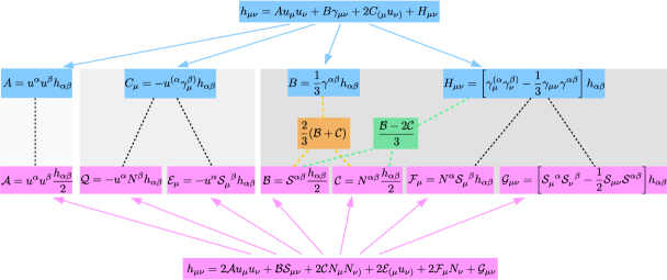
Figure 2: Relation between the degrees of freedom of the 1+3 and the 1+2+1 splittings. Capital upright letters refer to 1+3 splitting, while capital calligraphic letters refers to 1+2+1 spacetime splitting. Note that the variables ${\cal B}$ and ${\cal C}$ contribute both to a scalar mode ($B$) and to a transverse traceless mode $(H_{\mu\nu})$ of the 1+3 splitting. See the text for more details.

We call the reader’s attention to the algebraic mode coupling arising between the 1+2+1 scalars ${\cal B}$ and ${\cal C}$ and the 1+3 quantities $B$ and $H_{\mu\nu}$. Indeed, from (3.27) we see that two independent combinations of ${\cal B}$ and ${\cal C}$ will contribute to both $B$ and $H_{\mu\nu}$, which are quantities of rather different nature in the 1+3 splitting. We will come back to this issue in the next section since, as we shall see, it is central to our considerations.

We conclude this section by stressing that the above results are completely general, and can be applied to any spacetime whose topology of spatial sections are of the form $\Sigma_{\tau}={\cal M}^{2}\times\mathbb{R}$. For example, in ref. [50] the 1+2+1 splitting was used to investigate the evolution of gravitational waves in Schwarzschild spacetimes, where $\Sigma_{\tau}=\mathbb{S}^{2}\times\mathbb{R}$. Incidentally, note that the Schoolchild spacetime has the same spatial topology as the Kantowski-Sachs universe which we consider here. The main difference between these two spacetimes is in their set of isometries: the former describes an static and inhomogeneous spacetime, whereas the latter represents an expanding spatially homogeneous universe.

4 Gravitational waves

We now move on to one of our main tasks, which is the identification of the genuine tensor degrees of freedom in spacetimes with anisotropic curvature. As a warm up exercise — and also to elucidate the difficulties of this task — we briefly recall how this is done in FLRW universes in §4.2, after which we move to the more challenging cases of BIII and KS spacetimes in §4.3. Before that, though, we explore the conformally static character of the family of metrics (2.1) to simplify some of our calculations. More details can be found in Appendix §A.1.

4.1 Conformal transformation

Both spacetimes considered in this work are conformally related to a static (background) metric — see (2.1). In defining metric perturbations, it is wise to separate perturbations of the dynamic sector from those of the static one. We thus define

$$\delta g_{\mu\nu}\equiv h_{\mu\nu}\,,\qquad\text{and}\qquad\delta\widetilde{g}_{\mu\nu}\equiv a^{2}h_{\mu\nu}\,,$$ (4.1)

where $h_{\mu\nu}$ is given by either (3.4) or (3.17). Under a coordinate transformation of the form

$$x^{\mu}\rightarrow x^{\mu}-\xi^{\mu}\,,$$ (4.2)

where $\xi^{\mu}$ is the (infinitesimal) gauge vector,

$$\xi^{\mu}\equiv u^{\mu}T+J^{\mu}$$ (4.3)

each sector will transform as (see Appendix §A.1)

$$\delta g_{\mu\nu} \rightarrow\delta g_{\mu\nu}+2\nabla_{(\mu}\xi_{\nu)}\,,$$ (4.4)

$$\delta\widetilde{g}_{\mu\nu} \rightarrow\delta\widetilde{g}_{\mu\nu}+a^{2}\left(2\nabla_{(\mu}\xi_{\nu)}+2g_{\mu\nu}{\cal H}T\right)\,.$$ (4.5)

In the static sector many kinematical quantities are exactly zero, which makes the computation of (4.4) straightforward. The effect of the expansion can be later included by using (4.5). Indeed, in the static sector we have

$$K_{\mu\nu}=0=\dot{N}_{\mu}$$ (4.6)

which greatly simplifies the computation of gauge transformations. Once this is achieved, we can convert back to the dynamical sector by using (4.5) and the fact that (see §A.1)

$$\widetilde{K}_{\mu\nu} =a\left(K_{\mu\nu}+{\cal H}\gamma_{\mu\nu}\right)\,,$$

$$\widetilde{\nabla}_{\mu}\widetilde{N}_{\nu} =a\left(\nabla_{\mu}N_{\nu}+{\cal H}N_{\mu}u_{\nu}\right)\,.$$

4.2 FLRW case

In FLRW universes, the constant-time hypersurface $\Sigma_{\tau}$ describes a maximally symmetric submanifold and, as we have seen, the 1+3 spacetime splitting allow us to uniquely identify the tensor degrees of freedom of metric perturbations, $\delta g_{\mu\nu}$, with a traceless 3-tensor, such as $H_{\mu\nu}$ in (3.4). Note however that $H_{\mu\nu}$ has in general five degrees of freedom, three more than the two polarization states of gravitational waves. Such discrepancy, as is well known, is due to the fact that $H_{\mu\nu}$ is composed of fields of spin 0, 1 and 2, of which only the latter corresponds to true gravitational waves, while the other two correspond to pure gauge modes. Indeed, for a maximally symmetric subspace $\Sigma_{\tau}$, $H_{\mu\nu}$ can be uniquely decomposed as

$$H_{\mu\nu}=\left(D_{\mu}D_{\nu}-\frac{1}{3}\gamma_{\mu\nu}\nabla^{2}\right)2E+2D_{(\mu}E_{\nu)}+E_{\mu\nu}\,,$$ (4.7)

where

$$\nabla^{2}\equiv D^{\mu}D_{\mu}\,,\qquad D^{\mu}E_{\mu}=0=D^{\mu}E_{\mu\nu}\,.$$ (4.8)

This is the covariant formulation of the scalar-vector-tensor (SVT) decomposition, and is unique up to boundary conditions at infinity [53]. This decomposition splits the five components of $H_{\mu\nu}$ into one scalar $E$ (1 d.o.f), one divergence-free 3-vector $E_{\mu}$ (2 d.o.f) and one divergence-free and traceless 3-tensor $E_{\mu\nu}$ (2 d.o.f). The fact that both $E$ and $E_{\mu}$ are pure gauge modes can be seen by finding the 1+3 decomposition of the transformation (4.4). Using the conditions (3.10), plus the fact that $K_{\mu\nu}=0$ in the static sector of the metric, it is straightforward to show that

$$\delta g_{\mu\nu}\rightarrow\delta g_{\mu\nu}-2u_{\mu}u_{\nu}\dot{T}+2u_{(\mu}D_{\nu)}T+2D_{(\mu}J_{\nu)}-2u_{(\mu}\dot{J}_{\nu)}\,.$$ (4.9)

We now project both sides of this expression with $P_{\mu\phantom{\mu}\nu}^{\phantom{\mu}\alpha\phantom{\mu}\beta}$ (see eq. (3.7)) to find

$$H_{\mu\nu}\rightarrow H_{\mu\nu}+2D_{(\mu}J_{\nu)}-\frac{2}{3}\gamma_{\mu\nu}D^{\alpha}J_{\alpha}\,.$$ (4.10)

Next, we carry an SVT decomposition of the vector $J_{\alpha}$,

$$J_{\alpha}=D_{\alpha}L+L_{\alpha}\,,\quad\text{where}\quad D^{\alpha}L_{\alpha}=0\,,$$ (4.11)

and compare the result with (4.7). This gives

$$E \rightarrow E+L\,,$$

$$E_{\mu} \rightarrow E_{\mu}+L_{\mu}\,,$$ (4.12)

$$E_{\mu\nu} \rightarrow E_{\mu\nu}\,.$$

Finally, we need to change back to the dynamical perturbations $\delta\widetilde{g}_{\mu\nu}$ using (4.5). But since this is tantamount to adding a trace to (4.9), which goes away when projecting with $P_{\mu\phantom{\mu}\nu}^{\phantom{\mu}\alpha\phantom{\mu}\beta}$, we conclude that the transformations (4.12) hold in general. Clearly, $E$ and $E_{\mu}$ can be eliminated by going to a gauge where $L=-E$ and $L_{\mu}=-E_{\mu}$, whereas $E_{\mu\nu}$ remains gauge invariant. The 2 d.o.f in $E_{\mu\nu}$ represents the two polarizations of gravitational waves, and their equations of motion can be found by linearizing Einstein equations about the background metric. At this point it is convenient to adopt a comoving coordinate system given by

$$u_{\mu}=-\delta_{\mu}^{0}\,,\qquad\gamma_{\mu\nu}=\text{diag}\left(0,\gamma_{ij}\right)$$ (4.13)

and fix the gauge by choosing $E=0=E_{\mu}$, so that the most general line element for tensor perturbations about (2.1) reads

$${\rm d}s^{2} =a^{2}\left(g_{\mu\nu}+H_{\mu\nu}\right){\rm d}x^{\mu}{\rm d}x^{\nu}\,,$$

$$=a^{2}\left[-{\rm d}\eta^{2}+(\gamma_{ij}+E_{ij}){\rm d}x^{i}{\rm d}x^{j}\right]\,.$$

Note that we are allowed to focus on the evolution of $E_{\mu\nu}$ alone, since the other components of $\delta g_{\mu\nu}$ will not couple (either algebraically or dynamically) at first order. After a lengthy but well-known computation one then finds [52]

$$\ddot{E}{}_{ij}+2{\cal H}\dot{E}{}_{ij}-\nabla^{2}E_{ij}=0\,,$$ (4.14)

where, we remind the reader, dots represent derivatives with respect to conformal time.

Besides being damped by the expansion of the universe, the most remarkable feature of the equation above is that it holds for both polarization states. This is a direct consequence of the maximal symmetry of the background space, and, as we will see, no longer holds in the presence of anisotropic spatial curvature. For further reference, we note that in a radiation dominated universe where the scale factor evolves as $a=a_{0}\eta$, equation (4.14) has a regular solution at $\eta=0$ which in Fourier space is given by

$$E_{ij}(q,\eta)=C_{ij}\frac{\sqrt{q\eta}}{a(\eta)}J_{1/2}(q\eta)\,,$$ (4.15)

where $q$ is the Fourier wavenumber.

4.3 BIII and KS cases

The previous discussion relied on the identification of gravitational waves with the spin-2 and gauge-invariant components of metric perturbations. As we have seen, when $\Sigma_{\tau}$ is maximally symmetric we were able to define a unique component with these features (which we called $E_{\mu\nu}$), rendering the identification straightforward. If we tried to extend this program to the case $\Sigma_{\tau}=\mathcal{M}^{2}\times\mathbb{R}$, a naive guess would be to identify gravitational waves with $\mathcal{G}_{\mu\nu}$ since, as we have seen, it has 2 d.o.f and is the only traceless tensor related to $H_{\mu\nu}$ — which is known to contain gravitational waves d.o.f. There are however two serious problems with this approach. The first is that, in spacetimes with one privileged direction, the SVT decomposition (4.7) is no longer appropriate, and one has to resort instead to a scalar-vector (SV) decomposition which, by construction, cannot accommodate a divergence-free and traceless tensor like $E_{\mu\nu}$ [29]. This means that the two d.o.f originally contained in $E_{\mu\nu}$ have to be reallocated into the irreducible pieces of the SV decomposition, but a priori there is no way of guessing how to perform such task. Secondly, equations (3.27) and (3.28) show that there is an algebraic mode-coupling between 1+2+1 and 1+3 variables. This tell us that we cannot focus on the evolution of a particular mode and set the others to zero, as one does in deriving (4.14). In fact, a similar situation happens in Bianchi I spacetimes: when doing perturbation theory, one finds that vector perturbations have no dynamics, and arise only as a constraint between scalars and tensors [54]. Thus, even though vector modes do not grow as time evolves, they cannot be set to zero from the beginning, since this would lead to the wrong equations of motion for scalars and tensors.

In face of the above discussion, our approach here will be as follows: first, we move to the static sector and split (4.4) in the 1+2+1 fashion, keeping all its degrees of freedom. This will allow us to properly construct gauge-invariant variables and to find their correct equations of motion. Given these transformations we can use (3.19) to extract the transformation of the variables $(\mathcal{B}-\mathcal{C})$, ${\cal F}_{\mu}$ and ${\cal G}_{\mu\nu}$, which are directly related to $H_{\mu\nu}$ — see (3.28). This will tell us which of these behave as pure gauge modes, and which represent physical perturbations. Surprisingly, we will find that ${\cal G}_{\mu\nu}$ can be completely gauged away, which tell us that our naive guess aforementioned would be totally misplaced. We thus start by splitting (4.4) into 1+2+1 irreducible pieces. Actually, since (4.9) was already (1+3)-decomposed, all we need to do is to split its spatial components in its 2+1 pieces. To do that we write the gauge 3-vector $J_{\mu}$ as

$$J_{\mu}=\mathcal{J}N_{\mu}+\mathcal{J}_{\mu}\,,$$ (4.16)

where ${\cal J}_{\mu}N^{\mu}=0$. Next, we need to split the tensor $D_{(\mu}J_{\nu)}$ into its 2+1 components. First, we note that for any scalar field, and in particular for $\mathcal{J}$, we have $D_{\mu}\mathcal{J}=\mathcal{J}^{\prime}N_{\mu}+\mathcal{D}_{\mu}\mathcal{J}$ (recall the definitions made in (3.20)). Furthermore, we have

$$D_{\mu}\mathcal{J}_{\nu} =\gamma_{\mu}^{\phantom{\mu}\alpha}\gamma_{\nu}^{\phantom{\mu}\beta}D_{\alpha}\mathcal{J}_{\beta}\,,$$

$$=\mathcal{S}_{\mu}^{\phantom{\mu}\alpha}\mathcal{S}_{\nu}^{\phantom{\mu}\beta}D_{\alpha}\mathcal{J}_{\beta}+\mathcal{S}_{\mu}^{\phantom{\mu}\alpha}N_{\nu}N^{\beta}D_{\alpha}\mathcal{J}_{\beta}+N_{\mu}N^{\alpha}\gamma_{\nu}^{\phantom{\mu}\beta}D_{\alpha}\mathcal{J}_{\beta}\,,$$

$$=\mathcal{D}_{\mu}\mathcal{J}_{\nu}+N_{\mu}\mathcal{J}^{\prime}_{\nu}\,,$$

where we have used (3.24). Combining all the terms, using (3.23) and again (3.24), we find that

$$D_{\mu}J_{\nu}=\mathcal{J}^{\prime}N_{\mu}N_{\nu}+N_{\nu}\mathcal{D}_{\mu}\mathcal{J}+\mathcal{D}_{\mu}\mathcal{J}_{\nu}+N_{\mu}\mathcal{J}^{\prime}_{\nu}\,,$$ (4.17)

and, in particular, that $D_{\alpha}J^{\alpha}=\mathcal{J}^{\prime}+\mathcal{D}_{\alpha}\mathcal{J}^{\alpha}$. These equalities can now be used to rewrite (4.9) as

$$\delta g_{\mu\nu} \rightarrow\delta g_{\mu\nu}-2u_{\mu}u_{\nu}\dot{T}+2u_{(\mu}N_{\nu)}T^{\prime}+2u_{(\mu}{\cal D}_{\nu)}T-2u_{(\mu}N_{\nu)}\dot{{\cal J}}-2u_{(\mu}\dot{{\cal J}}_{\nu)}$$

$$\qquad\quad\;+2\mathcal{J}^{\prime}N_{\mu}N_{\nu}+2N_{(\mu}\mathcal{D}_{\nu)}\mathcal{J}+2\mathcal{D}_{(\mu}\mathcal{J}_{\nu)}+2N_{(\mu}\mathcal{J}^{\prime}_{\nu)}\,.$$

In deriving this transformation we have also used $\dot{N}_{\mu}=0$, which is true in the static sector. Using $\delta g_{\mu\nu}=h_{\mu\nu}$ and (3.19), the projection into 1+2+1 variables then gives

$${\cal A} \rightarrow{\cal A}-\dot{T}\,, \qquad{\cal E}_{\mu} \rightarrow{\cal E}_{\mu}+{\cal D}_{\mu}T-\dot{{\cal J}}_{\mu}\,,$$ (4.18)

$${\cal B} \rightarrow{\cal B}+{\cal D}_{\alpha}{\cal J}^{\alpha}\,, \qquad{\cal F}_{\mu} \rightarrow{\cal F}_{\mu}+\mathcal{D}_{\mu}\mathcal{J}+{\cal J}^{\prime}_{\mu}\,,$$

$${\cal C} \rightarrow{\cal C}+{\cal J}^{\prime}\,, \qquad{\cal G}_{\mu\nu} \rightarrow{\cal G}_{\mu\nu}+2{\cal D}_{(\mu}{\cal J}_{\nu)}-{\cal S}_{\mu\nu}{\cal D}_{\alpha}{\cal J}^{\alpha}\,.$$

$${\cal Q} \rightarrow{\cal Q}+T^{\prime}-\dot{{\cal J}}\,,$$

where we have also used ${\cal S}^{\prime}_{\mu\nu}=0$ and $\dot{{\cal S}}_{\mu\nu}=0$, the latter again being true for the static metric. At this point, the next logical step would be to carry the SVT decomposition of $\mathcal{E}_{\mu}$, $\mathcal{F}_{\mu}$, $\mathcal{J}_{\mu}$ and $\mathcal{G}_{\mu\nu}$. However $\mathcal{G}_{\mu\nu}$ cannot be decomposed in the same way as (4.7) since, in two dimensions, there is no nontrivial traceless and divergence-free 2-tensor. Nonetheless, we can still carry a SV decomposition as follows

$${\cal E}_{\mu} ={\cal D}_{\mu}\mathcal{E}+\widehat{\mathcal{E}}_{\mu}\,,\qquad\,\,\mathcal{D}_{\mu}\widehat{\mathcal{E}}^{\mu}=0\,,$$

$$\mathcal{J}_{\mu} =\mathcal{D}_{\mu}\mathcal{L}+\widehat{\mathcal{L}}_{\mu}\,,\qquad\,\mathcal{D}_{\mu}\widehat{\mathcal{L}}^{\mu}=0\,,$$

$$\mathcal{F}_{\mu} =\mathcal{D}_{\mu}\mathcal{F}+\widehat{\mathcal{F}}_{\mu}\,,\qquad\mathcal{D}_{\mu}\widehat{\mathcal{F}}^{\mu}=0\,,$$

$$\mathcal{G}_{\mu\nu} =2\Delta_{\mu\nu}\mathcal{G}+2\mathcal{D}_{(\mu}\widehat{\mathcal{G}}_{\nu)}\,,\qquad\mathcal{D}_{\mu}\widehat{\mathcal{G}}^{\mu}=0\,,$$

where $\Delta_{\mu\nu}\equiv\left(\mathcal{D}_{\mu}\mathcal{D}_{\nu}-\frac{1}{2}\mathcal{S}_{\mu\nu}\Delta^{2}\right)$ and $\Delta^{2}\equiv{\cal D}_{\alpha}{\cal D}^{\alpha}$. Plugging this decomposition into (4.18) and converting back to the dynamical perturbations $\delta\widetilde{g}_{\mu\nu}$, we finally find

$${\cal A} \rightarrow{\cal A}-\dot{T}-\mathcal{H}T\,, \widehat{\mathcal{E}}_{\mu} \rightarrow\widehat{\mathcal{E}}_{\mu}-\dot{\widehat{{\cal L}}}_{\mu}\,,$$ (4.19)

$${\cal B} \rightarrow{\cal B}+\Delta^{2}\mathcal{L}+2\mathcal{H}T\,, \widehat{\mathcal{F}}_{\mu} \rightarrow\widehat{\mathcal{F}}_{\mu}+\widehat{{\cal L}}^{\prime}_{\mu}\,,$$

$${\cal C} \rightarrow{\cal C}+{\cal J}^{\prime}+\mathcal{H}T\,, \widehat{\mathcal{G}}_{\mu} \rightarrow\widehat{\mathcal{G}}_{\mu}+\widehat{\mathcal{L}}_{\mu}\,.$$

$${\cal Q} \rightarrow{\cal Q}+T^{\prime}-\dot{{\cal J}}\,,$$

$${\cal E} \rightarrow{\cal E}+T-\dot{{\cal L}}\,,$$

$${\cal F} \rightarrow{\cal F}+\mathcal{J}+{\cal L}^{\prime}\,,$$

$${\cal G} \rightarrow{\cal G}+{\cal L}\,,$$

These completes the task of finding the general gauge transformation for 1+2+1 modes into scalar and vector components. From the above we can form the following gauge invariant variables:

$$\Phi \equiv-{\cal A}-\frac{1}{a}\left[a\left(\mathcal{E}+\dot{\mathcal{G}}\right)\right]^{\mbox{$\boldsymbol{\cdot}$}}\,, \;\Omega_{\mu} \equiv\widehat{\mathcal{F}}_{\mu}-\widehat{\mathcal{G}}^{\prime}_{\mu}\,,$$ (4.20)

$$2\Psi \equiv\mathcal{B}-2\mathcal{H}\left(\mathcal{E}+\dot{\mathcal{G}}\right)-\Delta^{2}\mathcal{G}\,, \Gamma_{\mu} \equiv\dot{\widehat{{\cal G}}}_{\mu}+\widehat{\mathcal{E}}_{\mu}\,,$$

$$\Pi \equiv\mathcal{Q}+\dot{\mathcal{F}}-\left(\mathcal{E}+2\dot{\mathcal{G}}\right)\,,$$

$$3X \equiv\left(\mathcal{B}-2\mathcal{C}\right)+2\left(\mathcal{F}-\mathcal{G}^{\prime}\right)^{\prime}-\Delta^{2}\mathcal{G}\,.$$

By the Stewart-Walker lemma [55], we know that (linearized) Einstein equations can be written in terms of these six variables. In practice, though, it is easier to work in the gauge where

$$\mathcal{E}=\mathcal{F}=\mathcal{G}=0=\widehat{\mathcal{G}}_{\mu}\,,$$ (4.21)

since the final equations can be trivially converted back to gauge invariant variables. Note also that this choice completely fix the gauge.

What about the gravitational waves d.o.f? From the last of eqs. (3.27) and the definitions (4.20), we can easily write $H_{\mu\nu}$ as a sum of gauge-dependent variables plus gauge-invariant terms:

$$H_{\mu\nu} =\frac{1}{3}\left[\Delta^{2}{\cal G}-2\left({\cal F}-{\cal G}^{\prime}\right)^{\prime}\right]\left(\mathcal{S}_{\mu\nu}-2N_{\mu}N_{\nu}\right)+2\left[{\cal D}_{(\mu}{\cal F}+\widehat{{\cal G}}^{\prime}_{\mu)}\right]N_{\nu}+{\cal G}_{\mu\nu}$$

$$+X\left(\mathcal{S}_{\mu\nu}-2N_{\mu}N_{\nu}\right)+2\Omega_{(\mu}N_{\nu)}\,.$$

This should be contrasted to (4.7). Clearly, $X$ and $\Omega_{\mu}$ represent the two physical perturbations we were looking for, whereas the remaining terms represent gauge (unphysical) modes. In the coordinate system defined by (4.21) we thus have

$$H_{\mu\nu}=X\left(\mathcal{S}_{\mu\nu}-2N_{\mu}N_{\nu}\right)+2\Omega_{(\mu}N_{\nu)}\,.$$ (4.22)

It is interesting to note that the mode ${\Gamma_{\mu}}$ does not contribute to gravitational waves. Indeed, it is not hard to convince oneself that the pairs $(\Phi,\Psi)$ on one hand and $(\Pi,\Gamma_{\mu})$ on the other correspond respectively to the two scalar and vector modes of standard (FLRW) perturbation theory. In fact, during inflation $\Pi$ and $\Gamma_{\mu}$ are dynamically suppressed while $\Psi$ and $\Phi$ become proportional to each other in the absence of anosotropic stress, just as in standard (FLRW) perturbation theory [29]. We have thus completed our first main task, which was to find the physical variables describing gravitational waves in BIII and KS spacetimes. It tell us that, when $\Sigma_{\tau}=\mathcal{M}^{2}\times\mathbb{R}$, the original spin-2 components of $H_{\mu\nu}$ now behaves as a spin-0 ($X$) and a spin-1 ($\Omega_{\mu}$) field. Qualitatively, this result is easy to understand. Since $\mathbb{R}$ is one dimensional, it only admits scalar propagating modes. Over $\mathcal{M}^{2}$ we can have both scalar and vector modes, but as we have seen, the scalar part turns out to be a pure gauge. Finally, note that there is no reason a priori to expect that these fields have the same dynamics and, as we shall see, they do not.

5 Dynamical equations and solutions

Equation (4.22) is the first main result of this work. Our second task is to find the equations of motion for $X$ and $\Omega_{\mu}$. As stressed before, because of algebraic couplings between scalar and vectors modes, these equations cannot be found by setting the other perturbations to zero, and we have to work with the most general metric perturbations. In the gauge (4.21), this is given by

$$\delta\widetilde{g}_{\mu\nu} =a^{2}h_{\mu\nu}$$

$$=-2\Phi u_{\mu}u_{\nu}+2\Psi{\cal S}_{\mu\nu}+(2\Psi-3X)N_{\mu}N_{\nu}+2\Pi N_{(\mu}u_{\nu)}+2\Gamma_{(\mu}u_{\nu)}+2\Omega_{(\mu}N_{\nu)}\,.$$

Adopting a coordinate system defined by

$$u_{\mu}=-\delta_{\mu}^{0}\,,\qquad\mathcal{S}_{\mu\nu}=\left(0,\mathcal{S}_{ab},0\right)\,,\qquad N_{\mu}=\delta_{\mu}^{z}\,,$$ (5.1)

where indices $a$, $b$ run from 1 to 2, the corresponding line element reads

$${\rm d}s^{2} =a^{2}\left[-(1+2\Phi){\rm d}\eta^{2}-2\Gamma_{a}{\rm d}^{a}x{\rm d}\eta-2\Pi{\rm d}z{\rm d}\eta\right.$$

$$\qquad\qquad\left.+\left(1+2\Psi\right)\mathcal{S}_{ab}{\rm d}x^{a}{\rm d}x^{b}+2\Omega_{a}{\rm d}x^{a}{\rm d}z+\left(1+2\Psi-3X\right){\rm d}z^{2}\right]\,.$$ (5.2)

This is the most general line element for linear perturbations in BIII and KS spacetimes, and it contains both scalar and vector perturbations. The linearized components of the Einstein tensor are presented in the Appendix A.3, together with the expressions for the linearized energy momentum tensor of the anisotropic scalar field, and we now focus on the construction of the equations of motion. Let us start by finding the equation for $X$. From eq. (A.20) we see that, in the absence of anisotropic stress in the perturbations of the perfect fluid, its scalar component obeys

$${\cal D}_{(a}{\cal D}_{b)}Z=0\,,\qquad\left(a\neq b\right)\,,$$ (5.3)

where $Z\equiv 2\Psi-3X+2\Phi$. Since this is the Killing equation, we can write ${\cal D}_{a}Z$ as

$${\cal D}_{a}Z=f_{i}(\eta,z)\zeta_{a}^{i}\,,$$ (5.4)

where the $\zeta_{a}^{i}$s are the three Killing vectors on ${\cal M}^{2}$. Given the explicit form of these vectors in a coordinate system, it is easy to show that partial derivatives of $Z$ will only commute if $f_{i}=0$, which then implies that $Z=0$ (see the appendix A.2 for a proof). We thus conclude that

$$2\Psi+2\Phi=3X\,.$$ (5.5)

Next, we subtract eq. (A.22) from the trace of eq. (A.20) and use (A.21) to eliminate $\Pi$. Using (5.5) this finally leads to

$$\ddot{X}+2{\cal H}\dot{X}-(\nabla^{2}+2\kappa)X=0\,,$$ (5.6)

which is the desired equation.

Next, we look for a dynamical equation for $\Omega_{a}$. From the vector component of eq. (A.20) we find ${\cal D}_{(a}Z_{b)}=0$, where $Z_{a}\equiv\Omega^{\prime}_{a}+\dot{\Gamma}_{a}+2{\cal H}\Gamma_{a}$ and $a\neq b$. Once more, this tell us that $Z_{a}=g_{i}(\eta,z)\zeta_{a}^{i}$ with arbitrary $g_{i}$. In the hyperbolic (BIII) case, the fact that cosmological perturbations go to zero at infinity fixes $g_{i}$ to zero, since there are no Killing vectors with this property [53]. In the spherical (KS) case there is no “spatial infinity” and $Z_{a}$ remains non-unique. However, it is clear that $g_{i}\zeta_{a}^{i}$ does not represent cosmological perturbations, and there is no loss of generality in again setting $g_{i}=0$. We thus use the constraint

$$\dot{\Gamma}_{a}+2{\cal H}\Gamma_{a}=-\Omega^{\prime}_{a}$$ (5.7)

in eq. (A.21), which allow us to obtain the following equation for the vector component:

$$\ddot{\Omega}_{a}+2{\cal H}\dot{\Omega}_{a}-\left(\nabla^{2}+\kappa\right)\Omega_{a}=0\,.$$ (5.8)

Equations (5.6) and (5.8) summarize our quest to find the dynamics of tensor perturbations in spacetimes with anisotropic curvature, and it is interesting at this point to compare them against eqs. (4.14). As we have anticipated, in the anisotropic case each mode has its own dynamics, the difference being more prominent at large cosmological scales, where the effect of the anisotropic curvature is larger. At small scales ($\nabla^{2}\gg\kappa$) the dynamics of the two modes become degenerate and we recover (4.14). Note however that this is not the only difference between these equations and the isotropic ones. In fact, the Laplacian in (5.6) and (5.8) have different spectra which appear as a different signatures in the power spectrum of each perturbation. We shall now investigate these issues in detail.

5.1 Spatial eigenfunctions

In order to solve the dynamical equations and evaluate the power spectra of gravitational waves we need to know how to perform Fourier analysis in spaces with anisotropic curvature. This requires knowledge of the eigenfunctions $\phi_{\mathbf{q}}$ of the Laplacian in these geometries, which are solutions of the eigenvalue problem

$$\nabla^{2}\phi_{\mathbf{q}}=-q^{2}\phi_{\mathbf{q}}\,,\qquad q\equiv\left|\mathbf{q}\right|\in\mathbb{R}^{+}\,.$$ (5.9)

For the metrics codified in (2.3) we have

$$\nabla^{2}=\kappa\left[\frac{1}{\sin\bar{\rho}}\partial_{\bar{\rho}}\left(\sin\bar{\rho}\,\partial_{\bar{\rho}}\right)+\frac{1}{\sin^{2}\bar{\rho}}\partial_{\varphi}^{2}+\partial_{\bar{z}}^{2}\right],$$ (5.10)

where $\bar{\rho}\equiv\sqrt{\kappa}\rho$ and $\bar{z}\equiv\sqrt{\kappa}z$. Note that for $\kappa=-\left|\kappa\right|$ this automatically gives the Laplacian of the BIII model. The eigenfunctions are given by [30, 33, 32]

$$\phi_{\mathbf{q}}\left(\mathbf{x}\right)=\begin{cases}N_{\ell m}P_{-1/2+i\ell}^{m}\left(\cosh\bar{\rho}\right)e^{im\varphi}e^{ik\bar{z}}\,,&\left(\text{BIII}\right)\\ N_{\ell m}P_{\ell}^{m}\left(\cos\bar{\rho}\right)e^{im\varphi}e^{ik\bar{z}}\,,&\left(\text{KS}\right)\end{cases}$$ (5.11)

where $k$ (not to be confused with the curvature parameter $\kappa$) is real, $m$ is an integer and $\ell$ is either real (BIII) or integer (KS), but always positive. These functions are orthonormal provided that we fix $N_{\ell m}$ as

$$N_{\ell m}=\frac{1}{2\pi}\begin{cases}\sqrt{(-1)^{m}\ell\tanh\pi\ell\frac{\Gamma\left(i\ell-m+1/2\right)}{\Gamma\left(i\ell+m+1/2\right)}}\,,&\left(\text{BIII}\right)\\ \sqrt{\frac{2\ell+1}{2}\frac{\left(\ell-m\right)!}{\left(\ell+m\right)!}}\,.&\left(\text{KS}\right)\end{cases}$$ (5.12)

One can also check that in the limit $\rho\ll 1$ and $\ell\gg 1$, $\phi_{\mathbf{q}}(\mathbf{x})$ becomes

$$\phi_{\mathbf{q}}(\mathbf{x})\approx\ell^{1/2}J_{m}(\ell\rho)\frac{e^{im\varphi}}{\sqrt{2\pi}}\frac{e^{ikz}}{\sqrt{2\pi}}$$ (5.13)

which, not surprisingly, are the eigenfunctions of a flat FLRW universe in cylindrical coordinates. Moreover, we notice that the eigenvalues $q^{2}$ are $m$-independent (reflecting the residual rotational symmetry of these geometries) and given by

$$q^{2}=\frac{1}{R_{c}^{2}}\begin{cases}\ell^{2}+k^{2}+\frac{1}{4}\,,&(\text{BIII},\,\ell\text{ real})\\ \left(\ell+1/2\right)^{2}+k^{2}-\frac{1}{4}\,,&(\text{KS},\,\ell\text{ integer})\end{cases}$$ (5.14)

where we have used (2.11). We thus see that, in both cases, $q$ has a fundamental lower bound given by

$$qR_{c}\equiv q_{*}\geq\begin{cases}(1/2)\,,&(\text{BIII})\\ \sqrt{2}\,.&(\text{KS})\end{cases}$$ (5.15)

As an aside, note that we can place observational bounds on $q$ using recent CMB data. The latest limits on the FLRW spatial curvature set by the Planck team and using CMB data alone gives $\Omega_{\kappa 0}=-0.005_{-0.017}^{+0.016}$ at 95% of confidence level [5]. This translates into

$$R_{c}\gtrsim 6.7H_{0}^{-1}\quad\text{(BIII)}\qquad\text{and}\qquad R_{c}\gtrsim 4.7H_{0}^{-1}\quad\text{(KS)}\,,$$ (5.16)

or, equivalently,

$$qH_{0}^{-1}\gtrsim 0.07\quad\text{(BIII)}\qquad\text{and}\qquad qH_{0}^{-1}\gtrsim 0.3\quad\text{(KS)}\,.$$ (5.17)

The fact that constraints on $R_{c}$ are weaker than those on $L_{c}$ (see eq. (2.11)) is a direct consequence of the (assumed) statistical anisotropy of the data. At large scales, where cosmic variance dominates, the temperature multipolar coefficients $a_{\ell m}$ with fixed $\ell$ and different $m$ become correlated [30], meaning that there is less constraining power in a given temperature spectrum $C_{\ell}$ than in the case of isotropic models

Given the eigenfunctions (5.11), any scalar perturbation $Q$ can be formally decomposed as

$$Q(\eta,\mathbf{x})=\int{\rm d}\mu_{\mathbf{q}}\,Q_{\mathbf{q}}(\eta)\phi_{\mathbf{q}}(\mathbf{x})\,,$$ (5.18)

with the inverse given by

$$Q_{\mathbf{q}}(\eta)=\int\sqrt{\gamma}{\rm d}^{3}\mathbf{x}\,Q(\eta,\mathbf{x})\phi_{\mathbf{q}}^{*}(\mathbf{x})\,.$$ (5.19)

Here, $\mu_{\mathbf{q}}$ formally represents the integration measure defined by the topology of each space (see [30] for the details). The decomposition of a transverse vector field $Q_{a}$ is essentially the same if we recognize that a transverse vector in two-dimensions is fundamentally a scalar field, and as such it can be written as

$$Q_{a}=\epsilon_{ab}{\cal D}^{b}Q$$ (5.20)

where $\epsilon_{ab}$ is the volume two-form on ${\cal M}^{2}$. Since $\epsilon_{ab}$ is covariantly conserved, this automatically ensures that ${\cal D}^{a}Q_{a}=0$. Thus, in practice we will always be working with scalars, and from now on we drop the index $a$ in any transverse vector. Before we proceed it is interesting to introduce two rescaled variables

$$x\equiv aX\,,\qquad\omega\equiv a\Omega\,,$$ (5.21)

in terms of which the equations of motion simplify (in Fourier space) to

$$\begin{split}\ddot{x}_{\mathbf{q}}+\left(q^{2}-\frac{\ddot{a}}{a}-2\kappa\right)x_{\mathbf{q}}&=0\,,\\ \ddot{\omega}_{\mathbf{q}}+\left(q^{2}-\frac{\ddot{a}}{a}-\kappa\right)\omega_{\mathbf{q}}&=0\,.\end{split}$$ (5.22)

Note that the frequency terms of these oscillators (i.e., the terms inside parenthesis) are fully isotropic, since they do not depend on $\mathbf{q}$, but only on its modulus. This is again a reflection of the isotropic background expansion, but also of the fact that the 1+2+1 splitting is adapted to the symmetries of the background space, so that no dynamical mode coupling arises. In particular, this implies that the quantization of the perturbations $x$ and $\omega$ during inflation will proceed along the same lines as the quantization of free fields in curved FLRW spaces [56], and that the power spectrum of each perturbation will only depend on $q$. We promptly stress, however, that the total power spectrum (i.e., the one defined through the complete tensor mode (4.22)) will certainly be a function of the full vector $\mathbf{q}$, rather than just $q$, since its definition requires that we fix the direction of the anisotropic curvature to some angle in the sky. In other words, we are still free to fix the orientation of $\mathbb{R}$ relative to ${\cal M}^{2}$. This will further imply in an anisotropic angular correlation function and in off-diagonal terms in, say, the CMB temperature covariance matrix [30]. We postpone a detailed analysis of these and other observables effects to a future work.

5.2 Solutions and power spectra

As a simple application of our results, let us find analytical solutions to eqs. (5.22) in some well known cosmological regimes. The simplest and most important case is that of radiation dominance for which $p_{f}=\rho_{f}/3$, for in that case equation (2.10) becomes simply

$$\frac{\ddot{a}}{a}=-\frac{\kappa}{2}=-\frac{\epsilon}{2R_{c}^{2}}\,,\qquad\epsilon=\text{sign}\left(\kappa\right)\,.$$ (5.23)

In this regime the scale factor evolves as

$$a(\eta)=a_{0}\begin{cases}\sqrt{2}R_{c}\sinh\left(\frac{\eta}{\sqrt{2}R_{c}}\right)&\left(\text{BIII, }\epsilon=-1\right)\,,\\ \sqrt{2}R_{c}\sin\left(\frac{\eta}{\sqrt{2}R_{c}}\right)&\left(\text{KS, }\epsilon=+1\right)\,,\end{cases}$$ (5.24)

where $a_{0}$ is an integration constant. Note that we have normalized these solutions so that $a(\eta)=a_{0}\eta$ when $R_{c}\gg 1$, which is the correct solution in the isotropic case. If we define $\beta^{2}\equiv 1-3\epsilon/2q_{*}^{2}$ and $\gamma^{2}\equiv 1-\epsilon/2q_{*}^{2}$, the regular solutions at $\eta=0$ are

$$X(q,\eta)=C_{1}\frac{\sqrt{q\eta}}{a(\eta)}J_{1/2}\left(\beta q\eta\right),\quad\Omega(q,\eta)=C_{2}\frac{\sqrt{q\eta}}{a(\eta)}J_{1/2}\left(\gamma q\eta\right),$$ (5.25)

where $C_{1,2}$ are integration constants. These solutions differ from those at eq. (4.15) in two aspects: first, the Bessel functions now have an explicit dependence on the curvature radius through the factors $\beta$ and $\gamma$, which in the isotropic case are both equal to one. Second, the scale factor now has a completely different behavior as the one of a flat FLRW radiation dominated universe. One particularly interesting consequence of these solutions is that, in a KS universe, the infinite wavelength perturbation of the tensor mode $X$ is constant in time. This happens because, in KS spaces, the largest wavelength has $q_{*}=\sqrt{2}$, which implies that $\beta=1/2$. Since $J_{1/2}(u/2)=2\sin\left(u/2\right)/(\sqrt{\pi u})$, we immediately find that $X=qC_{1}/a_{0}\sqrt{\pi}$ for all times. This is shown in figure (3) together with some other solutions for different values of the parameter $q_{*}$. For the sake of illustration we have adopted $qC_{1,2}/a_{0}=1$ in these plots.

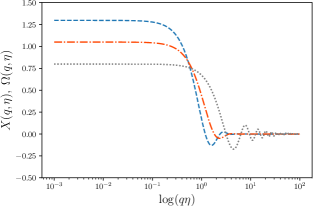
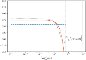
Figure 3: Evolution of the tensor modes $X$ (dashed line) and $\Omega$ (dot-dashed line) in BIII (left) and KS (right) models corresponding to the longest possible wavelength (see eq. (5.15)). The plots also show the evolution of the perturbations for $q_{*}=20$, in which case $X$ and $\Omega$ match the isotropic evolution. The vertical lines in the right panel represent the collapse time in the closed model for different curvature radii. Note that $X(q_{*}=\sqrt{2})$ is constant in the KS model for the whole evolution. See the text for details. For these plots we have set $qC_{1,2}/a_{0}=1$.

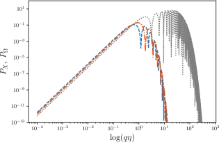
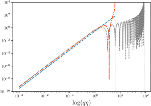
Figure 4: Power spectra $P_{X}$ and $P_{\Omega}$ of the tensor modes in BIII (left) and KS (right) models, with the same parameters values and coloring schemes as that of figure (3). Dashed vertical lines on the right panel represent the collapse time for each curvature radius. The amplitudes were arbitrarily set to one.

Because the dynamics of the modes $X$ and $\Omega$ is isotropic, we can define their power spectra simply as

$$P_{X}=q^{3}\left|X\left(q,\eta\right)\right|^{2}\,,\qquad P_{\Omega}=q^{3}\left|\Omega(q,\eta)\right|^{2}\,.$$ (5.26)

At large scales both $X$ and $\Omega$ are constant, and the power spectrum scales as $q^{3}$. As the mode crosses the Hubble horizon (i.e., at $q\eta\gtrsim 1$) the power at each perturbation scales nearly linearly with $q$. This goes on until the curvature affects the behavior of the scale factor, in which case the power will either decrease or increase, depending on whether the expansion goes on forever or faces a recollapse. This is shown numerically in figure (4).

6 Conclusions and final remarks

The detection of gravitational waves by the Ligo/Virgo collaboration opens a plethora of new opportunities for astrophysics and cosmology. While the direct detection of primordial gravitational waves might yet take a while, the impact of tensor perturbations in the temperature and polarization spectra of the CMB can already help us to constrain models of the early universe. In this work we have explored a particular class of models where the assumption of spatial isotropy is broken in such a way that the CMB remains isotropic at the background level. Such models offer an interesting example where the symmetries of the universe do not follow from the symmetries of the data, as one usually postulates. In particular, Bianchi type III and Kantowski-Sachs solutions with an imperfect-fluid matter content lead to the same expansion history as that of a curved Friedmann-Lemaître-Robertson-Walker universe. Here we have paid particular attention to the theoretical construction of linear gravitational waves in these models. In doing so, we found that the main difficulty is to separate physical from gauge degrees of freedom in the presence of anisotropic spatial curvature, which requires the use of a mode-splitting well adapted to the symmetries of the spacetime. Moreover, the presence of algebraic couplings between modes prevents one from ignoring perturbations not related to gravitational waves. In particular, had we kept only the $X$ and $\Omega_{a}$ variables in the expansion (5.2) we would end up with the wrong equations of motion.

Two specific signatures of gravitational waves arise in this context. First, the polarization modes of the wave behave as a spin-0 and spin-1 irreducible components of a transverse and traceless tensor, rather than two components of a spin-2 field. As such, each polarization has its own dynamics which differs from the usual (isotropic) case; the difference being larger at scales near the curvature radius. Second, the presence of a curvature radius in these models naturally implies in upper-limits to the size of a gravitational wave. In particular, we have found that the largest wave corresponding to the $X$-polarization mode in a KS universe is constant in time. However, such effect might easily be hidden in the stochastic background of gravitational radiation, and thus can be hard to detect.

We would like to conclude by commenting on a few applications of the formalism here presented. First, the integrated tensor Sachs-Wolfe effect predicts a variation in temperature given by $\Delta T/T=-\int e^{i}e^{j}\partial_{\eta}E{}_{ij}{\rm d}\eta$ [57]. Clearly, in the presence of anisotropic curvature it will get different contributions from the $X$- and $\Omega$-polarization modes, which will in turn affect the amplitude of the tensor spectrum at large CMB angles. Moreover, because there is an upper-limit to the maximum length of a wave, one should expect to find a deficit in the tensor spectrum at large angles, similarly to what happens with the tensor spectrum in closed FLRW universes [58]. Second, since the total power spectrum of tensor perturbations will depend on the direction of the vector $N^{\mu}$, one might expect anisotropies in the tensor/scalar ratio from inflation, which can be used as a further signature to discriminate these models. Lastly, one can also expect to find signatures coming from the direct effect of gravitational waves in the polarization of the $B$-modes of CMB. We postpone these analysis to a future work.

Appendix A Miscellanea

We gather here some useful formulae and results which were used in the main text.

A.1 Conformal transformations

We give here some details about the expressions involving conformal transformations. In the family of metrics in which we are interested, the dynamic (background) metric $\widetilde{g}_{\mu\nu}$ is conformally related to the static metric $g_{\mu\nu}$ through

$$\widetilde{g}_{\mu\nu}(x^{\lambda})=a^{2}g_{\mu\nu}(x^{\lambda})\,,\qquad\widetilde{g}^{\mu\nu}(x^{\lambda})=a^{-2}g^{\mu\nu}(x^{\lambda})\,,$$ (A.1)

where $a=a(\eta)$ is the scale factor and $x^{\lambda}=\left(\eta,\mathbf{x}\right)$. The proper time one-forms associated to each metric are related to each other through ${\rm d}\widetilde{\tau}=a{\rm d}\tau$. This further implies that

$$\widetilde{u}^{\mu}=\frac{dx^{\mu}}{d\widetilde{\tau}}=\frac{1}{a}\frac{dx^{\mu}}{d\tau}=a^{-1}u^{\mu}\,.$$ (A.2)

The following relations then follow from consistency

$$\widetilde{u}_{\mu}=au_{\mu}\,,\quad\widetilde{\gamma}_{\mu\nu}=a^{2}\gamma_{\mu\nu}\,,\quad\widetilde{N}_{\mu}=aN_{\mu}\,,\quad\widetilde{{\cal S}}_{\mu\nu}=a^{2}{\cal S}_{\mu\nu}\,.$$ (A.3)

However, note that $\widetilde{\gamma}_{\mu}^{\phantom{\mu}\nu}=\gamma_{\mu}^{\phantom{\mu}\nu}$ and $\widetilde{{\cal S}}_{\mu}^{\phantom{\mu}\nu}={\cal S}_{\mu}^{\phantom{\mu}\nu}$. Because both metrics describe homogeneous spacetimes, $\widetilde{\gamma}_{\mu}^{\phantom{\mu}\alpha}\widetilde{\nabla}_{\alpha}a=\widetilde{D}_{\mu}a=0$, which implies that

$$\widetilde{\nabla}_{\mu}a=-\widetilde{u}_{\mu}\widetilde{u}^{\alpha}\widetilde{\nabla}_{\alpha}a=-u_{\mu}u^{\alpha}\nabla_{\alpha}a=\nabla_{\mu}a\,.$$ (A.4)

In particular, in the comoving coordinate system of metric (2.1), $u^{\mu}=\left(1,0,0,0\right)$ and we have

$$\nabla_{\mu}a=-u_{\mu}\dot{a}\,,\quad\text{where}\quad\dot{a}=\frac{da}{d\eta}\,.$$ (A.5)

Given the gauge transformation of $\delta g_{\mu\nu}$, we can find that of $\delta\widetilde{g}_{\mu\nu}$ as follows:

$$\delta\widetilde{g}_{\mu\nu} \rightarrow\delta\widetilde{g}_{\mu\nu}+{\cal L}_{\xi}\left(\widetilde{g}_{\mu\nu}\right)\,,$$

$$=\delta\widetilde{g}_{\mu\nu}+a^{2}\left({\cal L}_{\xi}g_{\mu\nu}+2g_{\mu\nu}\frac{1}{a}\xi^{\alpha}\nabla_{\alpha}a\right)\,.$$

By writing $\xi^{\mu}=u^{\mu}T+J^{\mu}$ and using (A.4), it then follows that

$$\delta\widetilde{g}_{\mu\nu}\rightarrow\delta\widetilde{g}_{\mu\nu}+a^{2}\left({\cal L}_{\xi}g_{\mu\nu}+2g_{\mu\nu}\mathcal{H}T\right)\,,$$ (A.6)

where $\mathcal{H}=\dot{a}/a$ is the conformal Hubble function.

The derivatives $\widetilde{\nabla}_{\mu}$ and $\nabla_{\mu}$ will in general be different when acting on tensors, since

$$\widetilde{\Gamma}_{\mu\nu}^{\alpha} =\Gamma_{\mu\nu}^{\alpha}+\frac{1}{a}\left(2\delta_{(\mu}^{\alpha}\nabla_{\nu)}a-g_{\mu\nu}\nabla^{\alpha}a\right)\,,$$

$$=\Gamma_{\mu\nu}^{\alpha}-\left(2\delta_{(\mu}^{\alpha}u_{\nu)}-g_{\mu\nu}u^{\alpha}\right)\mathcal{H}\,.$$

In particular, this implies that the extrinsic curvature of the dynamic and static metric will be related by

$$\widetilde{K}_{\mu\nu}=\widetilde{\nabla}_{\mu}\widetilde{u}_{\nu}=a\left(K_{\mu\nu}+\mathcal{H}\gamma_{\mu\nu}\right)\,.$$ (A.7)

Likewise, the covariant derivative of vector $\widetilde{N}_{\mu}$ is given by

$$\widetilde{\nabla}_{\mu}\widetilde{N}_{\nu}=a\left(\nabla_{\mu}N_{\nu}+\mathcal{H}N_{\mu}u_{\nu}\right)\,.$$ (A.8)

A.2 Killing vectors on ${\cal M}^{2}$

Maximally symmetric two-dimensional manifolds of constant curvature can be represented by the following line element:

$${\rm d}s^{2}={\rm d}\rho^{2}+S_{\kappa}^{2}(\rho){\rm d}\varphi^{2}$$ (A.9)

where $S_{\kappa}(\rho)=\sin\left(\sqrt{\kappa}\rho\right)/\sqrt{\kappa}$. These spaces admit three Killing vectors:

$$\begin{split}\boldsymbol{\zeta}^{(1)}&=\partial_{\varphi}\,,\\ \boldsymbol{\zeta}^{(2)}&=\cos\varphi\partial_{\rho}-\sqrt{\kappa}\cot\left(\sqrt{\kappa}\rho\right)\sin\varphi\partial_{\varphi}\,,\\ \boldsymbol{\zeta}^{(3)}&=\sin\varphi\partial_{\rho}+\sqrt{\kappa}\cot\left(\sqrt{\kappa}\rho\right)\cos\varphi\partial_{\varphi}\,.\end{split}$$ (A.10)

Referring back to eq. (5.4) we see that

$$\partial_{\rho}Z=f_{2}\cos\varphi+f_{3}\sin\varphi\,,\qquad\partial_{\varphi}Z=f_{1}+\left(-f_{2}\sin\varphi+f_{3}\cos\varphi\right)\sqrt{\kappa}\cot\left(\sqrt{\kappa}\rho\right)\,.$$ (A.11)

Clearly, the equality $\partial_{\varphi}\partial_{\rho}Z=\partial_{\rho}\partial_{\varphi}Z$ will hold for arbitrary $\rho$ and $\varphi$ only when $f_{2}=f_{3}=0$. Moreover, since cosmological perturbations are defined as fluctuations above the mean, they don’t have a monopole. But $f_{1}$ is clearly a monopole, since it does not depend on $\rho$ and $\varphi$. Thus $f_{1}=0$. We thus conclude that $\partial_{\rho}Z=0=\partial_{\varphi}Z$, which implies that $Z$ is a constant. But since $Z$ cannot have a monopole, we conclude that $Z=0$.

A.3 Perturbed Einstein tensor

We give here a brief overview of linear perturbation theory. More details can be found in ref. [29]. As usual, we write the metric and its inverse as

$$g_{\mu\nu}\rightarrow g_{\mu\nu}+\delta g_{\mu\nu}\,,\qquad g^{\mu\nu}\rightarrow g^{\mu\nu}+\delta g^{\mu\nu}\,,$$ (A.12)

so that

$$\delta g^{\mu\nu}=-g^{\mu\alpha}g^{\nu\beta}\delta g_{\alpha\beta}\,.$$ (A.13)

In the coordinate system (2.3) we have

$$g_{00}=-a^{2}\,,\quad g_{ab}=a^{2}{\cal S}_{ab}\,,\quad g_{zz}=a^{2}$$ (A.14)

with inverse

$$g^{00}=-a^{-2}\,,\quad g^{ab}=a^{-2}{\cal S}^{ab}\,,\quad g^{zz}=a^{-2}\,.$$ (A.15)

Metric perturbations are parameterized as

$$\begin{split}\delta g_{00}&=-2a^{2}\Phi\,,\\ \delta g_{0a}&=-a^{2}\Gamma_{a}\,,\\ \delta g_{0z}&=-a^{2}\Pi\,,\\ \delta g_{ab}&=2a^{2}{\cal S}_{ab}\Psi\,,\\ \delta g_{az}&=a^{2}\Omega_{a}\,,\\ \delta g_{zz}&=a^{2}(2\Psi-3X)\,.\end{split}$$ (A.16)

These can be used to linearize all the tensors forming Einstein equations. The final result is

$$a^{2}\delta G_{\phantom{\mu}0}^{0} =6{\cal H}^{2}\Phi-2{\cal H}\Pi^{\prime}-3{\cal H}(2\dot{\Psi}-\dot{X})+\frac{1}{2}{\cal D}^{c}{\cal D}_{c}(4\Psi-3X)+2\kappa\Psi+2\Psi^{\prime\prime}$$

$$=a^{2}\delta T_{\phantom{\mu}0}^{0}\,,$$ (A.17)

$$a^{2}\delta G_{\phantom{\mu}a}^{0} ={\cal D}_{b}{\cal D}_{[a}\Gamma^{b]}-\frac{1}{2}\Gamma^{\prime\prime}_{a}-\kappa\Gamma_{a}-\frac{1}{2}\dot{\Omega}^{\prime}_{a}+\frac{1}{2}{\cal D}_{a}\Pi^{\prime}+\frac{1}{2}{\cal D}_{a}(4\dot{\Psi}-3\dot{X})-2{\cal H}{\cal D}_{a}\Phi$$

$$=a^{2}\delta T_{\phantom{\mu}a}^{0}\,,$$ (A.18)

$$a^{2}\delta G_{\phantom{\mu}z}^{0} =-2{\cal H}\Phi^{\prime}+2\dot{\Psi}^{\prime}-\frac{1}{2}{\cal D}^{a}{\cal D}_{a}\Pi=a^{2}\delta T_{\phantom{\mu}z}^{0}\,,$$ (A.19)

$$a^{2}\delta G_{\phantom{\mu}b}^{a} =\delta_{b}^{a}\left[2\Phi\left({\cal H}^{2}+2\dot{{\cal H}}\right)+2{\cal H}\dot{\Phi}+\Psi^{\prime\prime}-2{\cal H}\Pi^{\prime}-\frac{1}{2}(4\ddot{\Psi}-3\ddot{X})-{\cal H}(4\dot{\Psi}-3\dot{X})\right.$$

$$\left.+\Phi^{\prime\prime}-\dot{\Pi}^{\prime}+\frac{1}{2}{\cal D}^{c}{\cal D}_{c}(2\Psi-3X+2\Phi)\right]-\frac{1}{2}{\cal D}^{(a}{\cal D}_{b)}\left(2\Psi-3X+2\Phi\right)$$

$$+{\cal D}^{(a}\Omega^{\prime}_{b)}+{\cal D}^{(a}\dot{\Gamma}_{b)}+2{\cal H}{\cal D}^{(a}\Gamma_{b)}=a^{2}\delta T_{\phantom{\mu}b}^{a}\,,$$ (A.20)

$$a^{2}\delta G_{\phantom{\mu}a}^{z} =-{\cal D}_{a}\left(\Phi^{\prime}+\Psi^{\prime}\right)+{\cal H}{\cal D}_{a}\Pi+\frac{1}{2}{\cal D}_{a}\dot{\Pi}+{\cal H}\Gamma^{\prime}_{a}+\frac{1}{2}\dot{\Gamma}^{\prime}_{a}+\frac{1}{2}\ddot{\Omega}_{a}+{\cal H}\dot{\Omega}_{a}-\frac{\kappa}{2}\Omega_{a}-\frac{1}{2}{\cal D}^{c}{\cal D}_{c}\Omega_{a}$$

$$=a^{2}\delta T_{\phantom{\mu}a}^{z}\,,$$ (A.21)

$$a^{2}\delta G_{\phantom{\mu}z}^{z} =2\Phi({\cal H}^{2}+2\dot{{\cal H}})+2{\cal H}\dot{\Phi}+{\cal D}^{c}{\cal D}_{c}\left(\Phi+\Psi\right)-2\left(\ddot{\Psi}+2{\cal H}\dot{\Psi}-\kappa\Psi\right)$$

$$=a^{2}\delta T_{\phantom{\mu}z}^{z}\,.$$ (A.22)

We remind the reader that a dot and a prime means $\partial_{\eta}$ and $\partial_{z}$, respectively.

The non-zero perturbed components of the energy-momentum tensor are

$$a^{2}\delta T_{\phantom{\mu}0}^{0} =\kappa\left(-\Psi+3X/2+\delta\phi^{\prime}\right)\,,$$

$$a^{2}\delta T_{\phantom{\mu}z}^{0} =\kappa\left(\Pi+\delta\phi^{\prime}\right)\,,$$

$$a^{2}\delta T_{\phantom{\mu}b}^{a} =\kappa\left(-\Psi+3X/2+\delta\phi^{\prime}\right)\delta_{b}^{a}\,,$$

$$a^{2}\delta T_{\phantom{\mu}a}^{z} =-\kappa\,{\cal D}_{a}\delta\phi\,,$$

$$a^{2}\delta T_{\phantom{\mu}z}^{z} =\kappa\left(\Psi-3X/2-\delta\phi^{\prime}\right)\,.$$

Note that we are not perturbing the other components of the energy-momentum tensor. This is equivalent to the assumption that the perturbed anisotropic stress of the remaining fluids are negligible, which is a good approximation at large scales.

References

- [1] LIGO Scientific Collaboration and Virgo Collaboration collaboration, B. P. Abbott, R. Abbott, T. D. Abbott, M. R. Abernathy, F. Acernese, K. Ackley et al., Observation of gravitational waves from a binary black hole merger, Phys. Rev. Lett. 116 (Feb, 2016) 061102.
- [2] VIRGO, LIGO Scientific collaboration, B. P. Abbott et al., GW170104: Observation of a 50-Solar-Mass Binary Black Hole Coalescence at Redshift 0.2, Phys. Rev. Lett. 118 (2017) 221101, [1706.01812].
- [3] Virgo, LIGO Scientific collaboration, B. P. Abbott et al., GW151226: Observation of Gravitational Waves from a 22-Solar-Mass Binary Black Hole Coalescence, Phys. Rev. Lett. 116 (2016) 241103, [1606.04855].
- [4] WMAP collaboration, C. L. Bennett et al., Nine-Year Wilkinson Microwave Anisotropy Probe (WMAP) Observations: Final Maps and Results, Astrophys. J. Suppl. 208 (2013) 20, [1212.5225].
- [5] Planck collaboration, P. A. R. Ade et al., Planck 2015 results. XIII. Cosmological parameters, Astron. Astrophys. 594 (2016) A13, [1502.01589].
- [6] SPTpol collaboration, D. Hanson et al., Detection of B-mode Polarization in the Cosmic Microwave Background with Data from the South Pole Telescope, Phys. Rev. Lett. 111 (2013) 141301, [1307.5830].
- [7] BICEP2 collaboration, P. A. R. Ade et al., Detection of -Mode Polarization at Degree Angular Scales by BICEP2, Phys. Rev. Lett. 112 (2014) 241101, [1403.3985].
- [8] POLARBEAR collaboration, P. A. R. Ade et al., A Measurement of the Cosmic Microwave Background B-Mode Polarization Power Spectrum at Sub-Degree Scales with POLARBEAR, Astrophys. J. 794 (2014) 171, [1403.2369].
- [9] D. W. Hogg, D. J. Eisenstein, M. R. Blanton, N. A. Bahcall, J. Brinkmann, J. E. Gunn et al., Cosmic homogeneity demonstrated with luminous red galaxies, The Astrophysical Journal 624 (2005) 54.
- [10] Planck collaboration, P. A. R. Ade et al., Planck 2015 results. XVI. Isotropy and statistics of the CMB, Astron. Astrophys. 594 (2016) A16, [1506.07135].
- [11] P. Bull et al., Beyond CDM: Problems, solutions, and the road ahead, Phys. Dark Univ. 12 (2016) 56–99, [1512.05356].
- [12] J. García-Bellido and T. Haugboelle, Confronting Lemaitre-Tolman-Bondi models with observational cosmology, JCAP 0804 (2008) 003, [0802.1523].
- [13] S. Nadathur and S. Sarkar, Reconciling the local void with the CMB, Phys.Rev. D83 (2011) 063506, [1012.3460].
- [14] T. Biswas, A. Notari and W. Valkenburg, Testing the void against cosmological data: Fitting CMB, BAO, SN and H0, JCAP 1011 (2010) 030, [1007.3065].
- [15] C.-M. Yoo, K.-i. Nakao and M. Sasaki, CMB observations in LTB universes: Part I: Matching peak positions in the CMB spectrum, JCAP 1007 (2010) 012, [1005.0048].
- [16] L. Campanelli, P. Cea and L. Tedesco, Ellipsoidal universe can solve The CMB quadrupole problem, Phys.Rev.Lett. 97 (2006) 131302, [astro-ph/0606266].
- [17] A. Gümrükçüoğlu, C. R. Contaldi and M. Peloso, CMB anomalies from relic anisotropy, astro-ph/0608405.
- [18] A. Pontzen and A. Challinor, Bianchi model CMB polarization and its implications for CMB anomalies, Mon.Not.Roy.Astron.Soc. 380 (2007) 1387, [0706.2075].
- [19] D. C. Rodrigues, Anisotropic cosmological constant and the CMB quadrupole anomaly, Phys.Rev. D77 (2008) 023534, [0708.1168].
- [20] E. Martínez-González and J. Sanz, and the isotropy of the universe, Astron.Astrophys. 300 (1995) 346.
- [21] R. Maartens, G. F. Ellis and S. Stoeger, William R., Limits on anisotropy and inhomogeneity from the cosmic background radiation, Phys.Rev. D51 (1995) 1525, [astro-ph/9501016].
- [22] R. Maartens, G. F. Ellis and S. Stoeger, William R., Anisotropy and inhomogeneity of the universe from Delta(T) / T, Astron.Astrophys. 309 (1996) L7, [astro-ph/9510126].
- [23] C. Pitrou, T. S. Pereira and J.-P. Uzan, Predictions from an anisotropic inflationary era, JCAP 0804 (2008) 004, [0801.3596].
- [24] J. D. Barrow, R. Juszkiewicz and D. H. Sonoda, Universal rotation - How large can it be?, Mon. Not. Roy. Astron. Soc. 213 (1985) 917–943.
- [25] J. D. Barrow, P. G. Ferreira and J. Silk, Constraints on a primordial magnetic field, Phys. Rev. Lett. 78 (1997) 3610–3613, [astro-ph/9701063].
- [26] J. D. Barrow, Cosmological limits on slightly skew stresses, Phys. Rev. D55 (1997) 7451–7460, [gr-qc/9701038].
- [27] J. D. Barrow and R. Maartens, Anisotropic stresses in inhomogeneous universes, Phys. Rev. D59 (1999) 043502, [astro-ph/9808268].
- [28] J. D. Barrow and R. Maartens, Kaluza-Klein anisotropy in the CMB, Phys. Lett. B532 (2002) 153–158, [gr-qc/0108073].
- [29] T. S. Pereira, S. Carneiro and G. A. M. Marugan, Inflationary Perturbations in Anisotropic, Shear-Free Universes, JCAP 1205 (2012) 040, [1203.2072].
- [30] T. S. Pereira, G. A. M. Marugán and S. Carneiro, Cosmological Signatures of Anisotropic Spatial Curvature, JCAP 1507 (2015) 029, [1505.00794].
- [31] R. H. Brandenberger and C. Vafa, Superstrings in the Early Universe, Nucl. Phys. B316 (1989) 391–410.
- [32] J. J. Blanco-Pillado and M. P. Salem, Observable effects of anisotropic bubble nucleation, JCAP 1007 (2010) 007, [1003.0663].
- [33] J. Adamek, D. Campo and J. C. Niemeyer, Anisotropic Kantowski-Sachs Universe from Gravitational Tunneling and its Observational Signatures, Phys. Rev. D82 (2010) 086006, [1003.3204].
- [34] P. W. Graham, R. Harnik and S. Rajendran, Observing the Dimensionality of Our Parent Vacuum, Phys. Rev. D82 (2010) 063524, [1003.0236].
- [35] J. P. Mimoso and P. Crawford, Shear-free anisotropic cosmological models, Classical Quant. Grav. 10 (1993) 315.
- [36] A. A. Coley and D. J. McManus, On space-times admitting shear - free, irrotational, geodesic timelike congruences, Class. Quant. Grav. 11 (1994) 1261–1282, [gr-qc/9405034].
- [37] D. J. McManus and A. A. Coley, Shear - free irrotational, geodesic, anisotropic fluid cosmologies, Class. Quant. Grav. 11 (1994) 2045–2058, [gr-qc/9405035].
- [38] S. Carneiro and G. A. Mena Marugán, Anisotropic cosmologies containing isotropic background radiation, Phys.Rev. D64 (2001) 083502, [gr-qc/0109039].
- [39] S. Carneiro and G. A. Mena Marugán, An anisotropic cosmological model with isotropic background radiation, Lect. Notes Phys. 617 (2003) 302, [gr-qc/0203025].
- [40] J. Ehlers, P. Geren and R. K. Sachs, Isotropic solutions of the Einstein-Liouville equations, J. Math. Phys. 9 (1968) 1344.
- [41] C. A. Clarkson and R. Barrett, Does the isotropy of the CMB imply a homogeneous universe? Some generalized EGS theorems, Classical Quant. Grav. 16 (1999) 3781–3794, [gr-qc/9906097].
- [42] T. S. Koivisto, D. F. Mota, M. Quartin and T. G. Zlosnik, On the possibility of anisotropic curvature in cosmology, Phys.Rev. D83 (2011) 023509, [1006.3321].
- [43] S. Endlich, A. Nicolis and J. Wang, Solid Inflation, JCAP 1310 (2013) 011, [1210.0569].
- [44] N. Bartolo, S. Matarrese, M. Peloso and A. Ricciardone, Anisotropy in solid inflation, JCAP 1308 (2013) 022, [1306.4160].
- [45] M. Thorsrud, Balancing Anisotropic Curvature with Gauge Fields in a Class of Shear-Free Cosmological Models, to appear (2017).
- [46] V. Mukhanov, Physical Foundations of Cosmology. Cambridge University Press, Oxford, 2005.
- [47] S. W. Hawking, Perturbations of an expanding universe, Astrophys. J. 145 (1966) 544–554.
- [48] P. A. Hogan and G. F. R. Ellis, Propagation of information by electromagnetic and gravitational waves in cosmology, Classical and Quantum Gravity 14 (1997) A171.
- [49] P. K. S. Dunsby, B. A. C. C. Bassett and G. F. R. Ellis, Covariant analysis of gravitational waves in a cosmological context, Class. Quant. Grav. 14 (1997) 1215–1222, [gr-qc/9811092].
- [50] C. A. Clarkson and R. K. Barrett, Covariant perturbations of Schwarzschild black holes, Class. Quant. Grav. 20 (2003) 3855–3884, [gr-qc/0209051].
- [51] B. Osano, C. Pitrou, P. Dunsby, J.-P. Uzan and C. Clarkson, Gravitational waves generated by second order effects during inflation, JCAP 0704 (2007) 003, [gr-qc/0612108].
- [52] V. F. Mukhanov, H. A. Feldman and R. H. Brandenberger, Theory of cosmological perturbations. Part 1. Classical perturbations. Part 2. Quantum theory of perturbations. Part 3. Extensions, Phys. Rept. 215 (1992) 203.
- [53] J. M. Stewart, Perturbations of Friedmann-Robertson-Walker cosmological models, Classical Quant. Grav. 7 (1990) 1169.
- [54] T. S. Pereira, C. Pitrou and J.-P. Uzan, Theory of cosmological perturbations in an anisotropic universe, JCAP 0709 (2007) 006, [0707.0736].
- [55] J. M. Stewart and M. Walker, Perturbations of spacetimes in general relativity, Proc. Roy. Soc. Lond. A341 (1974) 49.
- [56] V. Mukhanov and S. Winitzki, Introduction to quantum effects in gravity. Cambridge University Press, 2007.
- [57] P. Peter and J.-P. Uzan, Primordial Cosmology . Oxford Graduate Texts. Oxford Univ. Press, Oxford, 2009.
- [58] B. Bonga, B. Gupt and N. Yokomizo, Tensor perturbations during inflation in a spatially closed Universe, JCAP 1705 (2017) 021, [1612.07281].