Reconstructing Generalized Staircase Polygons with Uniform Step Length

Abstract

Visibility graph reconstruction, which asks us to construct a polygon that has a given visibility graph, is a fundamental problem with unknown complexity (although visibility graph recognition is known to be in PSPACE). We show that two classes of uniform step length polygons can be reconstructed efficiently by finding and removing rectangles formed between consecutive convex boundary vertices called tabs. In particular, we give an $O(n^{2}m)$-time reconstruction algorithm for orthogonally convex polygons, where $n$ and $m$ are the number of vertices and edges in the visibility graph, respectively. We further show that reconstructing a monotone chain of staircases (a histogram) is fixed-parameter tractable, when parameterized on the number of tabs, and polynomially solvable in time $O(n^{2}m)$ under reasonable alignment restrictions.

1 Introduction

Visibility graphs, used to capture visibility in or between polygons, are simple but powerful tools in computational geometry. They are integral to solving many fundamental problems, such as routing in polygons, and art gallery and watchman problems, to name a few. Efficient, and even worst-case optimal, algorithms exist for computing a visibility graph from an input polygon [16]; however, comparatively little is known about the reverse direction: the so-called visibility graph recognition and reconstruction problems.

In this paper, we study vertex-vertex visibility graphs, which are formed by visibility between pairs vertices of a polygon. Given a graph $G=(V,E)$, the visibility graph recognition problem asks if $G$ is the visibility graph of some polygon. Similarly, the visibility graph reconstruction problem asks us to construct a polygon with $G$ as a visibility graph. Surprisingly, recognition of simple polygons is only known to be in PSPACE [13], and it is still unknown if simple polygons can be reconstructed in polynomial time. Therefore, current solutions are typically for restricted classes of polygons.

1.1 Special Classes

A well-known result due to ElGindy [11] is that every maximal outerplanar is a visibility graph and a polygon can be reconstructed from every such graph in polynomial time. Other special classes rely on a unique configuration of reflex and convex chains, which restrict visibility. For instance, spiral polygons [14], and tower polygons [7] (also called funnel polygons), can be reconstructed in linear time, and each consists of one and two reflex chains, respectively. $2$-spirals can also be reconstructed in polynomial time [3], as can a more general class of visibility graphs related to $3$-matroids [4].

For monotone polygons, Colley [8, 9] showed that if each face of a maximal outerplanar graph is replaced by a clique on the same number of vertices, then the resulting graph is a visibility graph of some uni-monotone polygon (monotone with respect to a single edge), and such a polygon can be reconstructed if the Hamiltonian cycle of the boundary edges is known. However, not every uni-monotone polygon (even those with uniformly spaced vertices) has such a visibility graph [12]. Finally, Evans and Saeedi [12] characterized terrain visibility graphs, which consist of a single monotone polygonal line.

For orthogonal polygons, orthogonal convex fans (also known as staircase polygons), which consist of a single staircase and an extra vertex, can be recognized in polynomial time [2]; however—strikingly—the only class of orthogonal polygons known to be reconstructible in polynomial time is the staircase polygon with uniform step lengths, due to Abello and Eğecioğlu [1]. Other algorithms for orthogonal polygons use different visibility representations such as vertex-edge or edge-edge visibility [18, Sect. 7.3], or “stabs” [17]. See Asano et al. [5] or Ghosh [15] for a thorough review of results on visibility graphs.

1.2 Our Results

In this work, we investigate reconstructing polygons consisting of multiple uniform step length staircases. We first show that orthogonally convex polygons can be reconstructed in time $O(n^{2}m)$. We further show that reconstructing orthogonal uni-monotone polygons is fixed-parameter tractable, when parameterized on the number of the horizontal convex-convex boundary edges in the polygon. We also provide an $O(n^{2}m)$ time algorithm under reasonable alignment assumptions. As a consequence of our reconstruction technique, we can also recognize the visibility graphs of these classes of polygons with the same running times.

2 Preliminaries

Let $P$ be a polygon on $n$ vertices. We say that a point $p$ sees a point $q$ (or $p$ and $q$ are visible) in polygon $P$ if the line segment $pq$ does not intersect the exterior of $P$. Under this definition, visibility is allowed along edges and through vertices.

For our visibility graph discussion, we adopt standard notation for graphs and polygons. In particular, for a graph $G=(V,E)$, we denote the neighborhood of a vertex $v\in V$ by $N(v)=\{u\mid(v,u)\in E\}$, and denote the number of vertices and edges by $n=|V|$ and $m=|E|$, respectively. For a visibility graph $G_{P}=(V_{P},E_{P})$ of a polygon $P$, we call an edge in $G_{P}$ that is an edge of $P$ a boundary edge. Other edges (diagonals in $P$) are non-boundary edges.

Finally, critical to our proofs is the fact that a maximal clique in $G_{P}$ corresponds to a maximal (in the number of vertices) convex region $R\subseteq P$ whose vertices are defined by vertices of $P$. A vertex $v$ is called simplicial if $N(v)$ forms a clique, or equivalently $v$ is in exactly one maximal clique. For our work here, we further adapt this definition for an edge. We say that an edge $(u,v)$ is $1$-simplicial if $N(u)\cap N(v)$ is a clique, or equivalently $(u,v)$ is in exactly one maximal clique. The intuition behind why we consider $1$-simplicial edges is that, in orthogonal polygons with edges of uniform length, boundary edges between convex vertices are $1$-simplicial, with the vertices of the clique forming a rectangle. (See Fig. 1.)

Our running times depend on the following observation for $1$-simplicial edges.

Observation 1

We can test if $(u,v)$ is $1$-simplicial and in a maximal $k$-clique in time $O(kn)$.

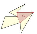
(a)

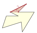
(b)

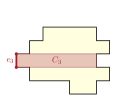
(c)

Figure 1: Maximal convex regions on vertices of polygons are maximal cliques in visibility graphs. (b)-(c) $1$-simplicial edges are in exactly one maximal clique.

3 Uniform-Length Orthogonally Convex Polygons

We first turn our attention to a restricted class of orthogonal polygons that have only uniform-length (or equivalently, unit-length) edges. Let $P$ be an orthogonal polygon with uniform-length edges such that no three consecutive vertices on $P$’s boundary are collinear, and further let $P$ be orthogonally convex. We call $P$ a uniform-length orthogonally convex polygon (UP). Note that every vertex $v_{i}$ on $P$’s boundary is either convex or reflex. We call boundary edges between two convex vertices in a uniform-length orthogonal polygon $P$ tabs and a tab’s endvertices tab vertices. We reconstruct the polygon by computing the clockwise ordering of vertices of the UP.

Note that the boundary of a UP consists of four tabs connected via staircases. For ease of exposition, we imagine the UP embedded in $\mathbb{R}^{2}$ with polygon edges axis-aligned. We call the tab with the largest $y$-coordinate the north tab, and we similarly name the others the south, east, and west tabs. We similarly refer to the four boundary staircases as northwest, northeast, southeast, and southwest.

We only consider polygons with more than $12$ vertices, which eliminates many special cases. Smaller polygons can be solved in constant time via brute force.

We first introduce several structural lemmas which help us identify convex vertices in a UP, which is key to our reconstruction.

Lemma 1

For every convex vertex $u$ in a UP there is a convex vertex $v$, such that $(u,v)\in E_{P}$ and $(u,v)$ is $1$-simplicial.

Proof

If $u$ is a tab vertex, then the other tab vertex $v$ is also convex and $(u,v)$ is $1$-simplicial. Otherwise, without loss of generality, suppose that $u$ is on the northwest staircase. Then there is a convex vertex $v$ on the southeast staircase that is visible from $u$. Edge $(u,v)$ is in exactly one maximal clique, consisting of $u$, $v$, the reflex vertices within the rectangle $R$ defined by $u$ and $v$ as the opposite corners, and any other corners of $R$ that are convex vertices of the polygon.

Lemma 2

In a UP, if $u$ or $v$ is a reflex vertex, then edge $(u,v)$ is not $1$-simplicial.

Proof (Sketch)

If both $u$ and $v$ are reflex, then $(u,v)$ is in one maximal clique consisting of only reflex vertices and another one that includes some convex vertex $w$. If one of $u$ or $v$ is convex, there exist two convex vertices $w$ and $w^{\prime}$, forming two distinct maximal cliques with $(u,v)$.

Lemma 2 states that only edges between convex vertices can be $1$-simplicial. Hence it allows us to identify all convex vertices, by checking for each edge $(u,v)$ if $N(u)\cap N(v)$ is a clique in $O(n^{2})$ time, leading to the following lemma.

Lemma 3

We can identify all convex and reflex vertices in a visibility graph of a UP in $O(n^{2}m)$ time.

We say a UP is regular if each of its staircase boundaries have the same number of vertices. Otherwise, we call it irregular, consisting of two long and two short staircases. We restrict our attention to irregular uniform-length orthogonally convex polygons (IUPs); however, similar methods work for their regular counterparts.

3.1 Irregular Uniform-Length Orthogonally Convex Polygons

Let $G_{P}$ be the visibility graph of IUP $P$. Our reconstruction algorithm first computes the four tabs, then assigns the convex and reflex vertices to each staircase. The following structural lemma helps us find the tabs. We assume that we have already computed the convex and reflex vertices in $O(n^{2}m)$ time.

Lemma 4

In every IUP there are exactly four $7$-vertex maximal cliques, each containing exactly three convex vertices. Each such clique contains exactly one tab, and each tab is contained in exactly one of these cliques.

Proof

First note that each of the four tabs are in exactly one such maximal $7$-clique. Further, any other clique that contains three convex vertices has at least nine vertices: each convex vertex and its two reflex boundary neighbors.

We note that it is not necessary to identify the four tabs explicitly to continue with the reconstruction. There are only $7^{4}=O(1)$ choices of tabs (one from each $7$-clique of Lemma 4), thus we can try all possible tab assignments, continue with the reconstruction and verify that our reconstruction produces a valid IUP $P$ with the same visibility graph. However, we can explicitly find the four tabs, giving us the following lemma.

Lemma 5

We can identify the four tabs of an IUP in $O(nm)$ time.

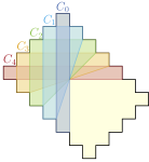
(a)

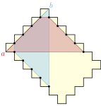
(b)

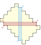
(c)

Figure 2: Elements of our reconstruction. (a) Elementary cliques $C_{0},\dots,C_{4}$ interlock along a short staircase. (b) Tab vertices $a$ and $b$ see unique reflex vertices on long staircases. (c) Reflex vertices (square) are discovered by forming rectangles with known vertices $u$, $v$ and $w$.

We pick one tab arbitrarily to be the north tab. We conceptually orient the polygon so that the northwest staircase is short and the northeast staircase is long. We do this by computing elementary cliques, which identify the convex vertices on the short staircase.

Definition 1 (elementary clique)

An elementary clique in an IUP is a maximal clique that contains exactly three convex vertices: one from a short staircase, and one from each of the long staircases. (See Fig. 2LABEL:sub@cliques.)

Lemma 6

We can identify the elementary cliques containing vertices on the northwest staircase in $O(nm)$ time.

Proof (Sketch)

Each elementary clique is constant size and contains a $1$-simplicial edge, and can therefore be discovered in $O(nm)$ time. Further, elementary cliques “interlock” along a staircase: each elementary clique shares exactly three reflex vertices with its at most two neighboring elementary cliques. Thus they can be computed starting from the elementary clique containing the north tab.

Note that, if our sole purpose is to reconstruct the IUP $P$, we have sufficient information. The number of elementary cliques gives us the number of vertices on a short staircase of the polygon, from which we can build a polygon. However, in what follows, we can actually map all vertices to their positions in the IUP, which we later use to build a recognition algorithm for IUPs.

First, we show how to assign all convex vertices from the elementary cliques to each of the three staircases, using visibility of the north and west tab vertices. Note, constructing the elementary cliques with Lemma 6 also gives us the west tab, since it is contained in the last elementary clique on the northwest staircase.

Lemma 7

We can identify the convex vertices on the northwest staircase in $O(n)$ time.

Proof

The northwest staircase contains the convex vertices of the elementary cliques from Lemma 6 that cannot be seen by any of the north or west tab vertices. The staircase further contains the left vertex of the north tab and the top vertex of the west tab (which can be identified by the fact that they are tab vertices that do not see either vertex of the other tab).

We can repeat the above process to identify the convex vertices of the southeast staircase. However, we might not yet be able to identify tabs as south or east. Thus, we will obtain two possible orderings of the convex vertices on the southeast staircase. Next, we show how to assign convex vertices to the long staircases. In the process we determine south and east tabs, and consequently, identify the correct ordering of convex vertices on the southeast staircase.

Lemma 8

We can assign the remaining convex vertices in $O(n^{2})$ time.

Proof (Sketch)

Let $v_{i},v_{i+1}$ be convex vertices on the same staircase, separated by a single reflex vertex. Let $u$ be the unique vertex on the opposite staircase, such that the angular bisector of $v_{i}$ goes through $u$. Then $u$ sees $v_{i+1}$. This likewise holds for the opposite staircase. Therefore, starting from one convex vertex on each staircase (such as a tab vertex), we can compute all convex vertices on each staircase.

Lemma 9

We can assign the reflex vertices to each staircase in $O(n^{2})$ time.

Proof (Sketch)

First we compare the reflex vertices seen by tab vertices, which gives us many vertices on the long staircases (see Fig. 2LABEL:sub@ab-visibility). The remaining reflex vertices are discovered by building vertical and horizontal rectangles that contain unassigned reflex vertices (see Fig. 2LABEL:sub@rectangles).

Observe that within each staircase, boundary edges are formed only between convex vertices and their reflex neighbors. Thus, we can order reflex vertices on each staircase by iterating over the staircase’s convex vertices (order of which is determined in Lemmas 6-8) and we are done. This gives us the following result:

Theorem 3.1

In $O(n^{2}m)$ time, we can reconstruct an IUP from its visibility graph.

4 Uniform-Length Histogram Polygons

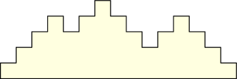
(a)

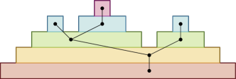
(b)

Figure 3: (a) A histogram $A$ with three tabs. (b) A decomposition of $A$ into touching rectangles with a contact graph that is a tree.

In this section we show how to reconstruct a more general class of uniform step length polygons: those that consist of a chain of alternating up- and down-staircases with uniform step length, which are monotone with respect to a single (longer) base edge. Such polygons are uniform-length histogram polygons [10], but we simply call them histograms for brevity (see Fig. 3LABEL:sub@monotone for an example). We refer to the two convex vertices comprising the base edge as base vertices. Furthermore, we refer to top horizontal boundary edges incident to two convex vertices as tab edges or just tabs and their incident vertices as tab vertices.

The case of two staircases.

We first note that in double staircase polygons (consisting of only two staircases) there is a simple linear-time reconstruction algorithm based on the degrees of vertices in the visibility graph. However, the construction relies on the symmetry of the two staircases and it is not clear whether any counting strategy works for arbitrary histograms.

4.1 Overview of the Algorithm

Every histogram can be decomposed into axis-aligned rectangles, whose contact graph is an ordered tree [10], as illustrated in Fig. 3LABEL:sub@tree. In Sect. 4.2, we show that we can construct the (unordered) contact tree $T$ from the visibility graph $G_{P}$ in $O(n^{2}m)$ time by repeatedly “peeling” tabs from the histogram. We then show that each left-to-right ordering of $T$’s $k$ leaves (as well as a left-to-right orientation of the rectangles in the leaves) induces a histogram $P^{\prime}$. For each candidate polygon $P^{\prime}$ (of $k!2^{k}$ candidates), we then compute its visibility graph $G_{P^{\prime}}$ in $O(n\log n+m)$ time [16] and check if $G_{P^{\prime}}$ is isomorphic to $G_{P}$. Instead of requiring an expensive graph isomorphism check [6], we show how to use the ordering of $T$ to quickly test if $G_{P}$ and $G_{P^{\prime}}$ are isomorphic.

In Sect. 4.4 we show how to reduce the number of candidate histograms from $k!2^{k}$ to $(k-2)!2^{k-2}$, leading to the main result of our paper:

Theorem 4.1

Given a visibility graph $G_{P}$ of a histogram $P$ with $k\geq 2$ tabs, we can reconstruct $P$ in $O(n^{2}m+(k-2)!2^{k-2}(n\log n+m))$ time.

Finally, we give a faster reconstruction algorithm when the histogram has a binary contact tree, solving these instances in $O(n^{2}m)$ time (Sect. 4.4).

4.2 Rectangular Decomposition and Contact Tree Construction

We construct the contact tree $T$ from $G_{P}$ by computing a set $\mathcal{T}$ of the $k$ tab edges of $G_{P}$ (Lemma 11). Each tab $(u,v)$ is $1$-simplicial and in a maximal $4$-clique, since $N(u)\cap N(v)$ is a $4$-clique representing a unit square at the top of the histogram. Given the set $\mathcal{T}$ of tab edges, our reconstruction algorithm picks an edge $t$ from $\mathcal{T}$ and removes the maximal $4$-clique containing $t$. This is equivalent to removing an axis-aligned rectangle in $P$, and, equivalently, removing a leaf node from $T$. Moreover, it associates that node of $T$ with four vertices of $P$: two top vertices that are convex and two bottom vertices that are either both reflex or are both convex base vertices. This process might result in a new tab edge, which we identify and add to $\mathcal{T}$.

4.2.1 Finding initial tabs.

We start by finding the $k$ tabs. Recall that every tab edge is $1$-simplicial and in a maximal $4$-clique. The converse is not necessarily true. Therefore, we begin by finding all $1$-simplicial edges that are in maximal $4$-cliques as a set of candidate edges, and later exclude non-tabs from the candidates.

Given a visibility graph $G_{P}=(V_{P},E_{P})$ of a histogram $P$ and a maximal clique $C\subseteq V_{P}$, we call a vertex $w\in C$ an isolated vertex with respect to $P$ if there exists a tab edge $(u,v)\in E_{P}$, such that $(N(u)\cup N(v))\cap C=\{w\}$, i.e., of all vertices of $C$, only $w$ is visible to some tab of $P$.

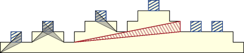
Figure 4: Illustrating all maximal $4$-cliques that contain $1$-simplicial edges. These include tab cliques (square regions) and non-tab cliques (triangular regions).

Lemma 10

In a histogram, every $1$-simplicial edge in a maximal $4$-clique contains either a tab vertex or an isolated vertex.

Proof (Sketch)

Figure 4 shows the only types of maximal $4$-cliques.

Lemma 11

In a visibility graph of a histogram, tabs can be computed in time $O(n^{2}m)$.

Proof (Sketch)

We find all maximal 4-cliques in $O(nm)$ by Observation 1 and detect and eliminate those containing isolated vertices in $O(n^{2}m)$ time.

Note that top vertices cannot see the vertices above them. Therefore, only bottom vertices see tab vertices. Moreover, every bottom vertex sees at least one tab vertex. Thus, identifying all tabs immediately classifies vertices of $G_{P}$ into top vertices and bottom vertices.

4.2.2 Peeling tabs.

Let $P^{\prime}$ be a polygon resulting from peeling tab cliques (rectangles) from a histogram $P$. We call $P^{\prime}$ a truncated histogram. See Fig. 5LABEL:sub@truncated for an example. After peeling a tab clique, the resulting polygon does not have uniform step length and the visibility graph may no longer have the properties on which Lemma 11 relied to detect initial tabs. Instead, we use the following lemma to detect newly created tabs during tab peeling.

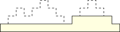
(a)

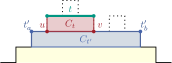
(b)

Figure 5: (a) A truncated histogram, created by iteratively removing six tabs (dashed) from a histogram. (b) When removing $C_{t}$: $t^{\prime}_{a},t^{\prime}_{b}$ form a tab iff $t^{\prime}_{a},t^{\prime}_{b}\in T\setminus C_{t}$, they see $u$ and $v$, and $|C_{t^{\prime}}|=4$.

Lemma 12

When removing a tab clique from the visibility graph of a truncated histogram, any newly introduced tab can be computed in time $O(n)$.

Proof

Denote the removed (tab) clique by $C_{t}$ and let $t$ be its tab. Let $u,v\not\in t$ be the non-tab vertices of $C_{t}$. Since $u$ sees $v$, $(u,v)$ is an edge in $G_{P}$.

Since top vertices can only see vertices at and below their own level, besides the vertices of $t$, there are exactly two other top vertices in (remaining) $G_{P}$ that see $u$ and $v$, namely, the top vertices $t^{\prime}_{a}$ and $t^{\prime}_{b}$ of $P$ on the same level as $u$ and $v$ (see Fig. 5LABEL:sub@tab-discovery). Since $t^{\prime}_{a},t^{\prime}_{b}$ are adjacent in $G_{P}$, let $t^{\prime}=(t^{\prime}_{a},t^{\prime}_{b})$.

When removing $C_{t}$ from $G_{P}$, we can compute $t^{\prime}_{a}$ and $t^{\prime}_{b}$ in time $O(n)$ by selecting the only two top vertices adjacent to both $u$ and $v$. Since $t^{\prime}_{a}$ and $t^{\prime}_{b}$ are the top vertices of a same rectangle $R_{t^{\prime}}$, edge $t^{\prime}$ is $1$-simplicial and is in exactly one maximal clique $C_{t^{\prime}}=N(t^{\prime}_{a})\cap N(t^{\prime}_{b})$, which corresponds to the convex region $R_{t^{\prime}}$. Finally, after $C_{t}$ is removed, $t^{\prime}$ is a newly created tab if and only if $|C_{t^{\prime}}|=4$, which can again be tested in time $O(n)$ by computing $N(t^{\prime}_{a})\cap N(t^{\prime}_{b})$.

With each tab clique (rectangle) removal, we iteratively build the parent-child relationship between the rectangles in the contact tree $T$ as follows. Using an array $A$, we maintain references to cliques being removed whose parents in $T$ have not been identified yet. When a tab clique $C_{t}$ is removed from $G_{P}$, the reference to $C_{t}$ is inserted into $A[u]$, where $u$ is one of the rectangle’s bottom vertices. If the removal of $C_{t}$ creates a new tab $t^{\prime}=(t^{\prime}_{a},t^{\prime}_{b})$, we identify $C_{t^{\prime}}$ in $O(n)$ time using Lemma 12. Recall that $t^{\prime}$ sees all bottom vertices on the same level. Thus, for every bottom vertex $u\in N(t^{\prime}_{a})$ (in the original graph $G_{P}$), if $A[u]$ is non-empty, we set $C_{t^{\prime}}$ as the parent of the clique stored in $A[u]$ and clear $A[u]$. This takes at most $O(n)$ time for each peeling of a clique. We get the following lemma, where the time is dominated by the computation of the initial tabs:

Lemma 13

In $O(n^{2}m)$ time we can construct the contact tree $T$ of $P$, associate with each $v\in T$ the four vertices that define the rectangular region of $v$, and classify vertices of $G_{P}$ as top vertices and bottom vertices.

4.3 Mapping Candidate Polygon Vertices to the Visibility Graph

Let $\hat{T}$ correspond to $T$ with some left-to-right ordering of its leaves and let $\hat{P}$ be the polygon corresponding to $\hat{T}$. We will map the vertices of $G_{P}$ to the vertices of $\hat{P}$ by providing for each vertex of $G_{P}$ the $x$- and $y$-coordinates of a corresponding vertex of $\hat{P}$. Let $t_{1},t_{2},\dots,t_{k}$ be the order of the tabs in $\hat{P}$. Since $\hat{T}$ unambiguously defines the polygon $\hat{P}$, each node $v$ of $\hat{T}$ is associated with a rectangular region on the plane, and the four vertices of $G_{P}$ are associated with the four corners of the rectangular region. Since by Lemma 13 every vertex of $G_{P}$ is classified as a top vertex or a bottom vertex, the $y$-coordinate can be assigned to all vertices unambiguously, because there are two top vertices and two bottom vertices associated with each node $v$ of $\hat{T}$. For every pair $p,\bar{p}$ of top vertices or bottom vertices associated with a node in $\hat{T}$ (we call them companion vertices) there is a choice of two $x$-coordinates: one associated with the left boundary and one associated with the right boundary of the rectangular region. Thus, determining the assignment of each top vertex and bottom vertex in $G_{P}$ to the left or the right boundary is equivalent to defining $x$-coordinates for all vertices in $G_{P}$. Although there appears to be $2^{n/2}$ possible such assignments, there are many dependencies between the assignments due to the visibility edges in $G_{P}$. In fact, we will show that by choosing the $x$-coordinates of the tab vertices, we can assign all the other vertices. Thus, in what follows we consider each of the $2^{k}$ possible assignments of $x$-coordinates to the $2k$ tab vertices.

At times we must reason about the assignment of a vertex to the left (right) staircases associated with some tab $t_{j}$. Given $\hat{T}$, the $x$-coordinates of each vertex in the left and right staircase associated with every tab $t_{j}$ is well-defined. Therefore, assigning a vertex $p$ to a left (right) staircase of some tab $t_{j}$ defines the $x$-coordinate of $p$.

In a valid histogram, companion vertices $p$ and $\bar{p}$ must be assigned distinct $x$-coordinates. Therefore, after each assignment below, we check the companion vertex and if they are both assigned the same $x$-coordinate, we exclude the current polygon candidate $\hat{P}$ from further consideration.

We further observe that in a valid histogram, if a bottom vertex $p$ is not in the tab clique, then it sees exactly one tab vertex, which lies on the opposite staircase associated with that tab. Thus, we assign every such bottom vertex the left (right) $x$-coordinate if it sees the right (left) tab vertex.

Next, consider any node $v$ of the contact tree $\hat{T}$ and let $R_{v}$ define the rectangle associated with $v$ in the rectangular decomposition of a valid histogram. Let $p$ be a top vertex in $R_{v}$ and let $S(p)$ be the set of vertices visible from $p$ that are not in $R_{v}$ ($S(p)$ can be determined from the neighborhood of $p$ in $G_{P}$). Observe that if $p$ is assigned the left (right) $x$-coordinate, then every vertex in $S(p)$ is a bottom vertex to the right (left) of the rectangle $R_{v}$, none of them belongs to a tab clique (i.e., all of them are already assigned $x$-coordinates), and all of them are assigned a right (left) $x$-coordinate. Since the $x$- and $y$-coordinates of the boundaries of $R_{v}$ are well-defined by $\hat{T}$ (regardless of vertex assignment), if $S(p)$ is non-empty, we check all of the above conditions and assign $p$ an appropriate $x$-coordinate. If a condition is violated, then the current polygon candidate is invalid and we exclude it from further consideration.

Let $p$ be one of the remaining top vertices without an assigned $x$-coordinate. If the companion $\bar{p}$ is assigned an $x$-coordinate, we assign $p$ the other choice of the $x$-coordinate. Otherwise, both $p$ and $\bar{p}$ see only the vertices inside their rectangle. In this case, the neighborhoods $N(p)$ and $N(\bar{p})$ are the same and we can assign $p$ and $\bar{p}$ to the opposite staircases arbitrarily.

Thus, the only remaining vertices without assigned $x$-coordinates are bottom vertices in tab cliques. Let $R$ be the rectangle defined by the tab and $S_{right}(p)$ (resp., $S_{left}(p)$) denote the set of vertices that $p$ sees among the vertices to the right (resp., left) of $R$. Consider a companion pair $p$ and $\bar{p}$ of bottom vertices that are in a tab clique. Observe that if $p$ is on the left boundary, then $S_{right}(\bar{p})\subseteq S_{right}(p)$ or $S_{left}(p)\subseteq S_{left}(\bar{p})$. Symmetrically, if $\bar{p}$ is on the left boundary then $S_{right}(p)\subseteq S_{right}(\bar{p})$ or $S_{left}(\bar{p})\subseteq S_{left}(p)$. Thus, if $|S_{right}(\bar{p})|\not=|S_{right}(p)|$ and $|S_{left}(p)|\not=|S_{left}(\bar{p})|$, we can assign $p$ and $\bar{p}$ appropriate $x$-coordinates. Otherwise, the neighborhoods $N(p)$ and $N(\bar{p})$ are the same, and we can assign $p$ and $\bar{p}$ to the opposite boundaries arbitrarily.

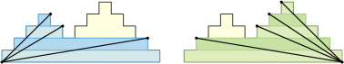
Figure 6: Visibility from the left (right) base vertex determines the left- (right-)most tab, and orients all rectangles on the left (right) spine of the contact tree.

4.4 Reducing the Number of Candidate Histograms

We can reduce the number of possible orderings of tabs and staircases by considering only those that meet certain visibility constraints on the vertices that form the corners of each rectangle. In particular, we say that two rectangles $R_{1}\neq R_{2}$ in the decomposition are orientation-fixed if a bottom vertex $v_{\mathrm{bot}}$ from one can see a top vertex $v_{\mathrm{top}}$ of another. Then these rectangles must be oriented so that $v_{\mathrm{bot}}$ and $v_{\mathrm{top}}$ are on opposite staircases (an up-staircase and a down-staircase). Thus, fixing an orientation of one rectangle fixes the orientation of the other.

Note that every rectangle is orientation-fixed with some leaf rectangle (as its bottom vertex can see a tab vertex). Therefore, ordering (and orienting) the leaves induces an ordering/orientation of the tree. There are $O(k!2^{k})$ such orderings (and orientations) for all leaf rectangles, where $k$ is the number of tabs.

For double staircases, $T$ is a path and the root rectangle is orientation-fixed with every other rectangle (a base vertex is seen by every top vertex). Hence, orienting the base rectangle determines the positions of the top vertices on the double staircase. Likewise, for the histogram, the spines of $T$ are fixed:

Lemma 14

The base rectangle of a histogram is orientation-fixed with all rectangles on the left and right spines of $T$.

Moreover, the only tab vertices visible from a base vertex are incident to the left-most or right-most tab. Thus, we can identify the left-most and right-most tabs based on the neighborhood of the base vertices. Note that removing a base rectangle of the histogram produces one or more histograms. Then we can apply this logic recursively, leading to the following algorithm:

1. Fix the orientation of the base rectangle. This identifies the rectangles on the left and right spines of $T$ and their orientations. (See Fig. 6.)

2. The remaining subtrees collectively contain the remaining rectangles, which still must be ordered and oriented. We recursively compute the ordering and orientation of the rectangles in these subtrees.

Note if we compute the left and right spines of $T$, we identify the first and last tabs, and the orientations of their tab edges. Thus, we have $(k-2)!2^{k-2}$ remaining orderings of $T$ and orientations of the tab edges to check, as $k-2$ tabs remain. This results in the overall reconstruction of a histogram with $k\geq 2$ tabs in $O(n^{2}m+(k-2)!2^{k-2}(n\log n+m))$ time, proving Theorem 4.1.

We now generalize the number of orderings to consider by defining a recurrence on the tree structure. Let $v\in T$, and define $C(v)$ be $v$’s children in $T$ and $d(v)=|C(v)|$. Then if we have a fixed orientation of $v$’s corresponding rectangle, fixing the rectangles on the left-most and right-most paths from $v$ limits the number of possible orderings/orientations of $v$’s descendants to

$$F(v)\leq\begin{cases}2^{d(v)-2}\prod_{u\in C(v)}{F(u)}&\text{if $d(v)>1$},\\ F(u)&\text{if $|C(v)|=1$, s.t. $C(v)=\{u\}$},\\ 1&\text{if $v$ is a leaf}.\end{cases}$$

Note that $F(root)=1$ for a binary tree $T$. That is, the orientation of the base rectangle completely determines the histogram. Furthermore, we can find such an orientation by fixing the orientation of the base edge, determining the left- and right-most paths, ordering and orienting them to match the base edge, and then repeating this for each subtree whose root is oriented and ordered (but its children are not), which acts as a base rectangle for its subtree. This process can be done in time $O(n+m)$ by traversing $T$ and orienting each rectangle exactly once by looking at its vertices neighbors in its base rectangle in $T$.

Theorem 4.2

Histograms with a binary contact tree can be reconstructed in $O(n^{2}m)$ time.

5 From Reconstruction to Recognition

We note that all of our reconstruction algorithms assign each vertex to a specific position in the constructed polygon. Let such an algorithm be called a vertex assignment reconstruction. As a result, we get recognition algorithms for these visibility graphs as well: we run our reconstruction until it fails or completes successfully, verify that the resulting polygon has the same visibility graph in time $O(n\log n+m)$ time [16], and verify that it is a polygon of the given type in linear time. Thus, we conclude that our reconstruction algorithms imply recognition algorithms with the same running times.

Appendix 0.A Omitted Proofs: Uniform-Length Orthogonally Convex Polygons

0.A.1 Proof of Lemma 2

To prove Lemma 2 we start with the following observations:

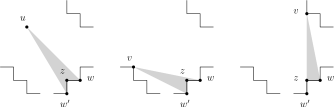
Figure 7: Illustration of the proofs of Observations 2 (left figure) and Observation 3 (middle and right) figures. Vertex $u$ on the northwest staircase can be reflex or convex.

Observation 2

If a vertex $u$ on the northwest staircase of an UP sees a reflex vertex $z$ on the southeast staircase and the slope of the line supporting the line segment $\overline{uz}$ is non-positive, then $u$ sees both (convex) boundary neighbors $w$ and $w^{\prime}$ of $z$.

Proof

We will prove that $w$, the horizontal boundary neighbor of $z$, is visible from $u$. Proof for visibility of $w^{\prime}$, the vertical boundary neighbor of $z$ is symmetric. See Fig. 7 (left) for an illustration.

First, observe that in an UP, no boundary edge on the northeast and the southwest staircases blocks visibility between the vertices of the northwest staircase and the vertices of the southeast staircase, and, consequently, between $u$ and $w$.

Next, by viewing $u$ as the origin of the Cartesian coordinate system, $z$ lies in the southeast quadrant (inclusive of the axis), because the slope of the line supporting $\overline{uz}$ is non-positive. And since $\overline{zw}$ is a horizontal edge, $w$ also lies in the southeast quadrant. Therefore, no boundary edge of the northwest staircase blocks the visibility between $u$ and $w$ (recall that our definition of visibility allows visibility along the polygon edges).

Finally, by viewing $w$ as the origin, we can similarly see that no edge of the southeast staircase blocks the visibility between $u$ and $w$.

Observation 3

Let a reflex vertex $v$ be on the southwest or northeast staircase of an UP and a reflex vertex $z$ be on the southeast staircase. If the slope of the line supporting the line segment $\overline{vz}$ is non-positive, then $v$ sees both (convex) boundary neighbors $w$ and $w^{\prime}$ of $z$.

Proof

Consider the case when $v$ is on the southwest staircase (the proof of the case when $v$ is on the northeast staircase is symmetric). See Fig. 7 (middle and right) for illustration.

First, observe that no boundary edge on the northwest and northeast staircase blocks the visibility between the vertices of the southwest staircase and the vertices of the southeast staircase, and, consequently, between $v$ and $w$.

Next, observe that the slope of the line supporting the edges from any reflex vertex on the southwest staircase and any vertex on the southeast staircase is at least $-\tan(\pi/4)$ and, therefore, no vertex on the southwest staircase can block the visibility between them.

Finally, by viewing $w$ (resp., $w^{\prime}$) as the origin of the Cartesian coordinate system, we can see that $v$ is in the northwest quadrant (inclusive of axis) and, therefore, no boundary edge on the southeast staircase can block the visibility between $w$ (resp., $w^{\prime}$) and $v$.

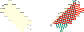
Figure 8: Illustration of the proof that an edge $(u,v)$ is non-simplicial, when both $u$ and $v$ are reflex. The proof demonstrates the existence of a convex vertex $w$ visible from both $u$ and $v$.

We are ready to prove Lemma 2.

Lemma 2.  In a UP, if $u$ or $v$ is a reflex vertex, then edge $(u,v)$ is not $1$-simplicial.

Proof

Let $(u,v)\in E_{P}$ and suppose that at least one of $u$ and $v$ is reflex.

Case 1: Both $u$ and $v$ are reflex. Then they belong to a maximal clique consisting of all reflex vertices and no convex vertices. We will show that both $u$ and $v$ also see some convex vertex $w$, therefore, $u,v$ and $w$ are part of another maximal clique. For concreteness of exposition, we orient the polygon so $u$ is always on the northwest staircase. There are two cases to consider:

1. Both $u$ and $v$ are on the short staircases. (See Fig. 8 (left)). Observe, that every reflex vertex on a short staircase sees all vertices on the other short staircase. Then, if $u$ and $v$ are on the same (northeast) staircase, there is a convex vertex $w$ on the southeast staircase, visible to both $u$ and $v$. If $v$ is on the southwest staircase, $w$ is either of the two convex boundary neighbors of $v$. Since $w$ is a boundary neighbor of $v$, clearly it is visible from $v$.

2. At least one of $u$ and $v$ is on a long staircase. (See Fig. 8 (right)). Without loss of generality, let it be $u$, which is on the northwest staircase. Vertex $u$ sees the right tab vertex $t_{r}$ of the north tab and the bottom tab vertex $t_{b}$ of the west tab. Since northwest staircase is long, the union of reflex vertices visible from $t_{r}$ and $t_{b}$ is the set of all reflex vertices in the polygon. Therefore, every reflex vertex $v$ must see at least one of $t_{r}$ or $t_{b}$.

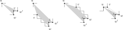
Figure 9: Illustration of the proof that an edge $(u,v)$ is non-simplicial, when one vertex, $u$, is convex and another, $v$, is reflex. For each of the four cases of when $v$ is on the four different staircases, there is a pair of convex vertices $w$ and $w^{\prime}$ on the southeast staircase, which are visible to both $u$ and $v$, but not to each other.

Case 2: One of the vertices is convex. Without loss of generality, let it be $u$ (again, on the northwest staircase), and let $v$ be reflex. Let $P_{u}$ be a polygon, which consists of $u$ and all reflex vertices visible from $u$. For every reflex vertex $v$ in $P_{u}$, we will identify two convex vertices $w$ and $w^{\prime}$ on the southeast staircase, which are visible to both $u$ and $v$. Since $w$ and $w^{\prime}$ are convex vertices on the same staircase, they are invisible to each other and, therefore, $u,v,w$ and $u,v,w^{\prime}$ will be part of two distinct maximal cliques.

Let us consider the four possible locations for $v$ (see Fig. 9 for illustrations):

1. $v$ is on the southeast staircase. Let $w$ and $w^{\prime}$ be the two convex boundary neighbors of $v$. Clearly, $v$ sees $w$ and $w^{\prime}$. Moreover, since $u$ sees $v$ and $v$ is on the opposite staircase from $u$, the slope of the line supporting the segment $\overline{uv}$ is non-positive. Then, by Observation 2, $u$ must also see $w$ and $w^{\prime}$.

2. $v$ is on the southwest staircase. Let $z$ be the lowest reflex vertex on the southeast staircase (adjacent to the south tab’s right vertex) and let $w$ and $w^{\prime}$ be the two convex boundary neighbors of $z$. Vertex $z$ is visible from $v$ because both $v$ and $z$ are reflex. Since $z$ is the lowest reflex vertex, the slope of the line supporting the segment $\overline{vz}$ is non-positive (the slope is 0 if $v$ is the lowest reflex vertex on the southwest staircase). Thus, by Observation 3, $w$ and $w^{\prime}$ are visible from $v$. Moreover, since $u$ sees $v$ and $v$ is on the southwest staircase, $z$ must be visible from $u$ with even smaller slope of the line supporting segment $\overline{uz}$, i.e., the slope is also non-positive. Therefore, by Observation 2, $w$ and $w^{\prime}$ are also visible from $u$.

3. $v$ is on the northeast staircase. Let $z$ be the highest reflex vertex on the southeast staircase (adjacent to the east tab’s bottom vertex) and let $w$ and $w^{\prime}$ be the two convex boundary neighbors of $z$. Again, vertex $z$ is visible from $v$ because both $v$ and $z$ are reflex. We can see that the slope of the line supporting the segment $\overline{vz}$ is negative by viewing $v$ as the origin of the Cartesian coordinate system and observing that $z$ is in the southeast quadrant. Thus, by Observation 3, $w$ and $w^{\prime}$ are visible from $v$. At the same time, $z$ is visible from $u$ because $v$ is visible from $u$ and $z$ is below and to the right of (or directly below) $v$. Moreover, the slope of the line supporting segment $uz$ is also non-positive. Therefore, by Observation 2, $w$ and $w^{\prime}$ are also visible from $u$.

4. $v$ is on the northwest staircase. Since $v$ is visible from $u$, $v$ must a reflex boundary neighbor of $u$. Observe, that because $P_{u}$ is bounded from all sides, it must contains a non-empty subset $Z$ of reflex vertices from the southeast staircase. Moreover, there exists a vertex $z\in Z$, which is not axis-aligned with $u$, i.e., the slope of the line supporting the segment $\overline{uz}$ is strictly negative. Let $w$ and $w^{\prime}$ be the two convex boundary neighbors of $z$. By definition of $P_{u}$, $z$ is visible from $u$, therefore, by Observation 2, $w$ and $w^{\prime}$ are visible from $u$. Again, $z$ is visible from $v$ because both $v$ and $z$ are reflex. Since the slope of the line supporting segment $\overline{uz}$ is strictly negative and the polygon has uniform length boundaries, the slope of the line supporting segment $\overline{vz}$ must be non-positive. Therefore, by Observation 2, $w$ and $w^{\prime}$ are also visible from $v$.

0.A.2 Proof of Lemma 5

Lemma 5.  We can identify the four tabs of an IUP in $O(nm)$ time.

Proof

We compute the four $7$-vertex maximal cliques of Lemma 4 in $O(nm)$ time using Observation 1. These cliques have exactly three convex vertices each, and tabs are incident to two convex vertices, narrowing our choice of tab down to $4\cdot\binom{3}{2}=12$ edges. Four of these are vertical or horizontal (non-boundary) edges, which we can detect and eliminate, as they are not $1$-simplicial: these edges are in both a clique with both tab vertices, and a clique containing a tab vertex, another convex vertex, and reflex vertices not in the tab clique. We have eight remaining edges to consider. These eight edges form four disjoint paths on two edges, and the middle vertex on each path is a tab vertex.

Note that these middle tab vertices are on the long staircases. Let one of them be called $u$. Now it remains to find $u$’s neighbor on its tab. Vertex $u$ has two candidate neighbors; let’s call them $v$ and $w$. Just for concreteness, let’s say $u$ is the vertex of the north tab on the northeast staircase.

Suppose, without loss of generality, that $v$ has more reflex neighbors than $w$, then $v$ is $u$’s neighbor on a tab, because it sees reflex vertices on the whole northeast and southeast staircases, while $w$ sees only a subset of those. Otherwise $v$ and $w$ have the same number of reflex neighbors, which only happens when $w$ sees every reflex vertex on the southeast and northeast staircases. Then either $v$ or $w$ has more convex neighbors. Suppose, without loss of generality, that $v$ is a tab vertex, then $v$ has fewer convex neighbors than $w$. To see why, note that since $u$ is on northeast (long) staircase, $v$ is on the northwest (short) staircase. Vertex $v$ has convex neighbors $u$, $w$, and every convex vertex on the southeast (short) staircase. Likewise, $w$ has convex neighbors $v$, $u$, every convex vertex on the northeast (long) staircase (including $u$) and one vertex on the southeast (short) staircase.

We can do these checks for all such pairs $v$ and $w$, giving us all tabs. Note that, if we have already distinguished convex and reflex vertices, this step takes time $O(nm)$: $O(nm)$ time to compute the four cliques containing tabs, and $O(n)$ to count the number of reflex and convex vertices visible from each tab vertex candidate.

0.A.3 Proof of Lemma 6

Lemma 6.  We can identify the elementary cliques containing vertices on the northwest staircase in $O(nm)$ time.

Proof

Each elementary clique $C$ contains a $1$-simplicial edge, as $C$ is maximal and two convex vertices in $C$ must be on opposite staircases. Using Observation 1 we compute all $1$-simplicial edges in maximal cliques on seven or nine vertices in $O(nm)$ time, and keep the cliques that are elementary cliques—those that contain three convex and either four or six reflex vertices.

Let $k_{NW}$ be the number of convex vertices on the northwest staircase. We number these convex vertices from $v_{0}$ to $v_{k_{NW}-1}$ in order along the northwest staircase from the north tab to the west tab. We denote by $C_{i}$ the unique elementary clique containing $v_{i}$. Note that $C_{0}$ is the unique maximal (elementary) clique containing the north tab. Furthermore, each clique $C_{i}$ contains a set of reflex vertices $R_{i}$ such that $|R_{i}\cap C_{i+1}|=3$, and for $j\not\in\{i-1,i,i+1\}$, $R_{i}\cap C_{j}=\emptyset$. Therefore, from elementary clique $C_{i}$, we can compute elementary clique $C_{i+1}$ by searching for the only other elementary clique containing reflex vertices $R_{i}$. Once we reach an elementary clique containing a tab, then we have computed all elementary cliques on the northwest staircase. This tab is the west tab and we are finished.

0.A.4 Proof of Lemma 8

Lemma 8.  We can assign the remaining convex vertices in $O(n^{2})$ time.

Proof

Let $\mathcal{W}$ and $\mathcal{E}$ be all the convex vertices on the southwest and northeast staircases (which we are computing) and let $\mathcal{W}_{0}$ and $\mathcal{E}_{0}$ be the convex vertices on the southwest and northeast staircases that are already known from the elementary cliques from Lemma 7. Let $N_{c}(v)$ denote the set of convex neighbors on the opposite staircase of some vertex $v$. Then, for each vertex $w_{0}\in\mathcal{W}_{0}$, $N_{c}(w_{0})\subseteq\mathcal{E}$, i.e., the convex neighbors of the (convex) vertices in $\mathcal{W}_{0}$ are on the northeast staircase. Similarly, for each vertex $e_{0}\in\mathcal{E}_{0}$, $N_{c}(e_{0})\subseteq\mathcal{W}$. Then we can iteratively define sets $\mathcal{E}_{i}=(\cup_{w\in\mathcal{W}_{i-1}}N_{c}(w))\setminus\mathcal{E}_{i-1}$ and $\mathcal{W}_{i}=(\cup_{e\in\mathcal{E}_{i-1}}N_{c}(e))\setminus\mathcal{W}_{i-1}$ and identify all vertices of the southwest and northeast staircases as $\mathcal{W}=\cup_{i}\mathcal{W}_{i}$ and $\mathcal{E}=\cup_{i}\mathcal{E}_{i}$.

To order the vertices along the southwest staircase, note that the sets $\mathcal{W}_{i}$ should appear in order of increasing $i$ from top to bottom. Also note that if one were to assign the vertices of $\mathcal{W}_{i}$ to a staircase from top to bottom, each vertex $w_{i}$ in this order would see fewer vertices of $\mathcal{E}_{i-1}$. Thus, we can order the vertices within each $\mathcal{W}_{i}$. The argument for ordering vertices of $\mathcal{E}_{i}$ is symmetric.

Computing set $\mathcal{E}_{i}$ takes time $O(|\mathcal{W}_{i-1}|\cdot n)$: we evaluate all $O(n)$ neighbors of each neighbor in $\mathcal{W}_{i-1}$. Likewise, computing $\mathcal{W}_{i}$ takes time $O(|\mathcal{E}_{i-1}|\cdot n)$. Thus, overall it takes $O((|\mathcal{W}|+|\mathcal{E}|)\cdot n)=O(n^{2})$ time to construct (and order) sets $\mathcal{W}$ and $\mathcal{E}$.

0.A.5 Proof of Lemma 9

Lemma 9.  We can assign the reflex vertices to each staircase in $O(n^{2})$ time.

Proof

Once the convex vertices are ordered on the staircases, we can compare the reflex vertices that are seen from the tab vertices. Let $a$ and $b$ be vertices on different tabs visible along a short staircase (see Fig. 2LABEL:sub@ab-visibility). Let $\mathcal{R}$ be the set of all reflex vertices of the IUP, and $N(v)$ be a set of all neighbors of vertex $v$ in the visibility graph of IUP. Then $\mathcal{R}_{0}=N(a)\cap N(b)\cap\mathcal{R}$ contains all reflex vertices from the short staircase, plus two extra reflex vertices from its neighboring long staircases. The remaining vertices $N(a)\setminus\mathcal{R}_{0}$ are on one long staircase (and $N(b)\setminus R_{0}$ are on the other long staircase).

Thus, we can find many reflex vertices on the long staircases in $O(n)$ time, except the endvertices and potentially those in the middle of the staircases. To find the remaining ones, we build rectangles (maximal cliques) consisting of two convex vertices $u$ and $v$ on the opposite staircases and a known reflex vertex $w$, such that $(u,w)$ forms a boundary edge of the IUP (see Fig. 2LABEL:sub@rectangles). These rectangles define new reflex vertices on the staircase opposite from $w$. Thus, we iteratively discover all new reflex vertices.

Given the two convex vertices of the rectangle, it takes $O(n)$ to compute the maximal $6$-clique of the rectangle, and $O(1)$ to determine the new reflex vertex. We must do this for $O(n)$ rectangles. Hence, the total time to discover these new reflex vertices is $O(n^{2})$.

Appendix 0.B Omitted Proofs: Histograms

0.B.1 Reconstructing a Double Staircase Polygon in Linear Time

Every double staircase polygon can be decomposed into $k$ axis-aligned rectangles for some integer $k\geq 1$. Note that the number of vertices in such polygon is $4k$, with each vertex $u$ on one of $k+1$ levels $l_{u}=0,\dots,k$. With the exception of levels $l_{u}=0$ and $l_{u}=k$, which contain only two vertices (pairs of tab and base vertices), there are four vertices per level (two top and two bottom vertices).

Observe that the degree $deg(u)$ of each vertex $u\in G_{P}$ exhibits the following pattern:

1. $u_{k}$ is a tab vertex (on level $k$). $deg(u_{k})=k+2$: $u_{k}$ is a neighbor to $k$ bottom vertices on the opposite staircase and two boundary vertices of $u$.

2. $u_{l}$ is a top vertex on level $l=1,\dots,k-1$. $deg(u_{l})=l+4$: $u_{l}$ is a neighbor to $l+1$ bottom vertices on the opposite staircase, 1 convex vertex on the same level as $u_{l}$ on the opposite staircase, and two boundary vertices of $u_{l}$.

3. $u_{l}$ is a bottom vertex on level $l=1,\dots,k-1$. $deg(u_{l})=3k-l+2$: $u_{l}$ is a neighbor to $k$ bottom vertices on the opposite staircase, $k-l+1$ top vertices on the opposite staircase, $k-1$ bottom vertices on the same staircase and two boundary vertices of $u_{l}$.

4. $u_{0}$ is a base vertex (on level $0$). $deg(u_{0})=3k$: $u_{0}$ is a neighbor to $2k$ vertices on the opposite staircase, $k-1$ bottom vertices on the same staircase, and one boundary vertex of $u_{0}$.

Observe, that most of the above values for degrees come in pairs: one vertex per staircase. For positive integer $k$, the only two exceptions are $deg(u)=k+2$ and $deg(u)=3k$, each of which appears four times: two tab vertices $u_{k}$ and $u^{\prime}_{k}$ and two top vertices $u_{k-2}$ and $u^{\prime}_{k-2}$ (on level $k-2$), and two base vertices $u_{0}$ and $u^{\prime}_{0}$ and two bottom vertices $u_{2}$ and $u^{\prime}_{2}$ (on level $2$). However, we can easily differentiate tab vertices $u_{k}$ and $u^{\prime}_{k}$ from top vertices $u_{k-2}$ and $u^{\prime}_{k-2}$, because $u_{k}$ and $u^{\prime}_{k}$ are neighbors to the two bottom vertices on level $k-1$ (of degree $2k+3$), while $u_{k-2}$ and $u^{\prime}_{k-2}$ are not. Similarly, we can differentiate the two base vertices $u_{0}$ and $u^{\prime}_{0}$ from bottom vertices $u_{2}$ and $u^{\prime}_{2}$, because $u_{0}$ and $u^{\prime}_{0}$ are neighbors to the two top vertices on level one (of degree $5$), while $u_{2}$ and $u^{\prime}_{2}$ are not.

Thus, we can identify the levels of each vertex by their degrees (or the degrees of their neighbors). Finally, an arbitrary left-right assignment of the two base vertices to the two staircases, defines the assignment of all top (convex) vertices (including tab vertices) to the staircase. The assignment of tab vertices to the staircases defines the assignment of all reflex vertices to staircases. Such assignment can be performed in linear time using the classification of the vertices into top and bottom vertices based on their degrees.

0.B.2 Proof of Lemma 10

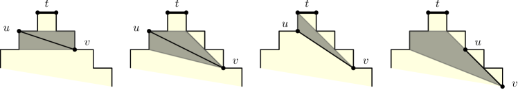
Figure 10: Edges between $u,v$ on a tab $t$’s staircases, but disjoint from $t$, are in a clique of size at least $5$.

Lemma 10.  In a histogram, every $1$-simplicial edge in a maximal $4$-clique contains either a tab vertex or an isolated vertex.

Proof

Let $\ell_{u}$ denote the level of vertex $u$ in $P$, which is its $y$-coordinate assuming all uniform edges have unit length, where the base vertices are at level 0. Consider an arbitrary $1$-simplicial edge $(u,v)$ that is part of a maximal $4$-clique $C$. We assume that neither $u$ nor $v$ is a tab vertex, otherwise we are done. Note that if $|\ell_{u}-\ell_{v}|\leq 1$ then $u$ and $v$ are in an axis-aligned rectangle in $P$ defined by at least six vertices of $G_{P}$ and thus $|C|\geq 6$. Thus, suppose that $\ell_{u}-\ell_{v}\geq 2$ and, without loss of generality, $u$ lies to the right of $v$ (the case of $u$ lying to the left of $v$ can be proven symmetrically). Since a top vertex does not see any vertices above it, $v$ must be a bottom vertex. Thus, $v$ sees a vertex of some tab $t$. We will show that $t$ cannot see any other vertex of $C$. Let $R$ be a set of reflex vertices on $v$’s staircase on levels $\ell_{v}+1$ up to and including $\ell_{u}$. Observe, that $v$ cannot be part of the maximal $4$-clique that contains both vertices of $t$, hence, $1\leq|R|\leq\ell_{u}-\ell_{v}$ ($|R|<\ell_{u}-\ell_{v}$ when the vertices of $t$ are below $u$).

Case 1: $u$ and $v$ are vertices of an up- and down-staircase of $t$. (See Fig. 10.)

1. $u$ is a top vertex: $u$ and $v$ must lie on different staircases, and $(u,v)$ is in a clique consisting of $u$, $(\ell_{u}-\ell_{v})$ reflex vertices on $v$’s staircase, $v$, and $u$’s two (reflex) boundary neighbors and thus $|C|\geq 6$.

2. $u$ is a bottom vertex: Then $(u,v)$ is in a convex quadrilateral (clique) consisting of at least five vertices: $(\ell_{u}-\ell_{v}+1)\geq 3$ bottom vertices on $v$’s (up-)staircase from levels $\ell_{v}$ through $\ell_{u}$, and on the opposite (down-)staircase: a bottom vertex on level $\ell_{u}$ and top vertex on level $\ell_{u}+1$.

Case 2: Vertices $u$ and $v$ belong to up- and down-staircases of different tabs. Then we call $(u,v)$ a crossing edge. Consider the following cases:

1. $u$ is reflex: Let $(u,u^{\prime})$ be a horizontal boundary edge.

   1. $u^{\prime}$ is convex: Let $(u^{\prime},u^{\prime\prime})$ be a vertical boundary edge. Then $v$ sees $u^{\prime\prime}$, $C=\{v,u,u^{\prime},u^{\prime\prime}\}$ and $t$ does not see $u,u^{\prime},$ or $u^{\prime\prime}$.

   2. $u^{\prime}$ is reflex: Either some vertex in $R$ sees $u$ and $u^{\prime}$ (and, consequently, is in $C$) or there is a vertex $w\in C$, such that line segments $\overline{vw}$ and $\overline{wu}$ define the boundary of the convex region of $C$ which exclude the vertices of $R$. At the same time, there must be at least one vertex $w^{\prime}\in C$, bounding the convex region of $C$ on the right (e.g. by line segments $\overline{u^{\prime}w^{\prime}}$ and $\overline{w^{\prime}v}$. Either way, $|C|>4$.

2. $u$ is convex: Let $(u,u^{\prime})$ and $(u^{\prime\prime},u)$ be the vertical and horizontal boundary edges, respectively. Since $v$ sees $u$ and $u^{\prime}$ is below $u$, $v$ must see $u^{\prime}$, i.e. $u^{\prime}\in C$, but $t$ does not see $u^{\prime}$.

   1. $v$ does not see $u^{\prime\prime}$: There must be a reflex vertex $w\in C$, that blocks $v$ from seeing $u^{\prime\prime}$. Note that $u$ sees both $v$ and $u^{\prime\prime}$ and consequently cannot belong to $v$’s double staircase, i.e. $t$ does not see $w$. Thus $C=\{v,u,u^{\prime},w\}$ and $t$ sees $v$, but not $u$, $u^{\prime}$, or $w$.

   2. $v$ sees $u^{\prime\prime}$: In this case, either some vertices of $R$ are in $C$ or there is some other vertex $w\in C$ blocking them from $u$, $u^{\prime}$ or $u^{\prime\prime}$. In either case, since $\{v,u,u^{\prime},u^{\prime\prime}\}\subsetneq C$, $|C|>4$.

0.B.3 Proof of Lemma 11

Lemma 11.  In a visibility graph of a histogram, tabs can be computed in time $O(n^{2}m)$.

Proof

See Fig. 4. We begin by computing all $1$-simplicial edges in maximal $4$-cliques, which takes time $O(n^{2}m)$ by Observation 1. Call this set of edges $E_{\mathrm{sim}}$, and the set of their maximal cliques $\mathcal{C}_{\mathrm{sim}}$. Then $E_{\mathrm{sim}}$ contains the tabs, some edges that share a vertex with the tabs, and edges between staircases of different tabs (crossing edges) (which contain isolated vertices by Lemma 10). For all (non-incident) pairs of $1$-simplicial edges $e_{1}$ and $e_{2}$ in maximal $4$-cliques $C_{1}$ and $C_{2}$, respectively, we check if exactly one vertex of $C_{2}$ can be seen by an endvertex of $e_{1}$. That is, we compute the set $V_{12}=\{v\in C_{2}\mid(u,v)\in E\text{ and }u\in e_{1}\}$ and verify that $|V_{12}|=1$. If $e_{1}$ is a tab, then $C_{2}$ contains an isolated vertex, and is detected as a non-tab clique. Thus, if we compare all pairs of edges and cliques, all $4$-cliques containing crossing edges will be eliminated. We can do this check in $O(nm)$ time by first storing, for each vertex $u$, the edges $\{(u,v)\in E_{\mathrm{sim}}\}$ and cliques $\{C\in\mathcal{C}_{\mathrm{sim}}\mid u\in C\}$. Then for each edge $(u,v)$ in $G_{P}$, we run the isolated vertex check for each pair of edges and cliques stored at the endvertices $u$ and $v$. Each check of all pairs takes $O(n^{2})$, and we do this for $|E_{\mathrm{sim}}|=O(m)$ edges.

If only disjoint cliques remain after the previous step, then we have computed exactly all $k$ tabs. Otherwise, we need to eliminate non-tab edges that share a tab vertex. Note that non-tab edges form cliques along the staircase incident to the tab. Since staircases in a histogram are disjoint, non-tab cliques only intersect where they intersect a tab clique. Therefore, the remaining set of cliques can be split into $k$ mutually disjoint sets, where $k$ is the number of top tabs, and each set has at most three cliques that intersect (see Fig. 4), of which exactly one is a tab clique, and the other at most two cliques contain a tab vertex, and its non-tab neighbors on the opposite staircase. Let $S$ be one of these $k$ sets. We can compute the tab in $S$ as follows (three cases):

1. ($|S|=1$) Then the tab vertices see fewer vertices than non-tab (reflex) vertices. We can see this as follows: tab vertices see the vertices in their tab clique, plus the bottom vertices on the tab’s staircases. The non-tab reflex vertices see the same vertices, plus at least two other vertices at their same level, which tab vertices cannot see.

2. ($|S|=2$) The two cliques in $S$ share three vertices, and two vertices $u$ and $v$ that are in exactly one unique clique each. One of these vertices (say $u$) is on the tab, and sees fewer vertices than the other non-tab vertex ($v$) does. We can see this as follows: assume without loss of generality that $u$ is on the left of its double staircase. Then $u$ sees the three vertices of its tab clique, and all reflex vertices on the left staircase. Meanwhile $v$ is on the same side (left) as $u$, and sees the same vertices as $u$, plus a (convex) boundary neighbor, which is on the level between $u$ and $v$, which $u$ cannot see. The remaining tab vertex is adjacent to $v$ along its $1$-simplicial edge forming the clique in $S$.

3. ($|S|=3$) The cliques intersect in a symmetric pattern. The tab edge is formed between the two vertices that are in exactly two of these maximal cliques.

There are at most $3k=O(n)$ of these overlapping cliques in total, and they can be separated into their respective $k$ disjoint sets in time $O(k)$ by marking the vertices of each set, and collecting the intersecting sets. Then within each set, it takes $O(1)$ time to find the tab. Thus the running time is dominated by the time to detect crossing edges in $E_{\mathrm{sim}}$: $O(n^{2}m)$.

References

- [1] J. Abello and Ö. Eğecioğlu. Visibility graphs of staircase polygons with uniform step length. International Journal of Computational Geometry & Applications, 03(01):27–37, 1993.
- [2] J. Abello, Ö. Eğecioğlu, and K. Kumar. Visibility graphs of staircase polygons and the weak Bruhat order, I: From visibility graphs to maximal chains. Discrete Comput. Geom., 14(3):331–358, 1995.
- [3] J. Abello and K. Kumar. Visibility graphs of 2-spiral polygons (extended abstract). In R. Baeza-Yates, E. Goles, and P. V. Poblete, editors, Proc. 2nd Latin American Symposium, volume 911 of LNCS, pages 1–15. Springer, 1995.
- [4] J. Abello and K. Kumar. Visibility graphs and oriented matroids. Discrete & Computational Geometry, 28(4):449–465, 2002.
- [5] T. Asano, S. K. Ghosh, and T. C. Shermer. Chapter 19–visibility in the plane. In J.-R. S. J. Urrutia, editor, Handbook of Computational Geometry, pages 829–876. North-Holland, Amsterdam, 2000.
- [6] L. Babai. Graph isomorphism in quasipolynomial time [extended abstract]. In Proc. 48th ACM Symposium on Theory of Computing, STOC ’16, pages 684–697, New York, NY, USA, 2016. ACM.
- [7] S.-H. Choi, S. Y. Shin, and K.-Y. Chwa. Characterizing and recognizing the visibility graph of a funnel-shaped polygon. Algorithmica, 14(1):27–51, 1995.
- [8] P. Colley. Visibility graphs of uni-monotone polygons. Master’s thesis, Department of Computer Science, University of Waterloo, Waterloo, Canada, 1991.
- [9] P. Colley. Recognizing visibility graphs of unimonotone polygons. In Proc. 4th Canad. Conf. Comput. Geom., pages 29–34, 1992.
- [10] S. Durocher and S. Mehrabi. Computing partitions of rectilinear polygons with minimum stabbing number. In J. Gudmundsson, J. Mestre, and T. Viglas, editors, Proc. 18th Annual International Conference on Computing and Combinatorics (COCOON 2012), volume 7434 of LNCS, pages 228–239. Springer, 2012.
- [11] H. ElGindy. Hierarchical decomposition of polygons with applications. PhD thesis, McGill University, Montreal, Canada, 1985.
- [12] W. Evans and N. Saeedi. On characterizing terrain visibility graphs. J. Comput. Geom., 6(1):108–141, 2015.
- [13] H. Everett. Visibility graph recognition. PhD thesis, University of Toronto, 1990.
- [14] H. Everett and D. Corneil. Recognizing visibility graphs of spiral polygons. J. Algorithms, 11(1):1–26, 1990.
- [15] S. K. Ghosh. Visibility Algorithms in the Plane. Cambridge University Press, 2007.
- [16] S. K. Ghosh and D. M. Mount. An output-sensitive algorithm for computing visibility. SIAM J. Comput., 20(5):888–910, Oct. 1991.
- [17] L. Jackson and S. Wismath. Orthogonal polygon reconstruction from stabbing information. Comp. Geom.-Theor. Appl., 23(1):69–83, 2002.
- [18] J. O’Rourke. Art Gallery Theorems and Algorithms. Oxford University Press, New York, 1987.