From the reaction
to the production of pairs
in ultraperipheral ultrarelativistic heavy-ion collisions at the LHC
Mariola Kłusek-Gawenda
Mariola.Klusek@ifj.edu.plInstitute of Nuclear Physics Polish Academy of Sciences, Radzikowskiego 152, PL-31-342 Kraków, Poland
Piotr Lebiedowicz
Piotr.Lebiedowicz@ifj.edu.plInstitute of Nuclear Physics Polish Academy of Sciences, Radzikowskiego 152, PL-31-342 Kraków, Poland
Otto Nachtmann
O.Nachtmann@thphys.uni-heidelberg.deInstitut für Theoretische Physik, Universität Heidelberg,
Philosophenweg 16, D-69120 Heidelberg, Germany
Antoni Szczurek
111Also at Faculty of Mathematics and Natural Sciences, University of Rzeszów, Pigonia 1, PL-35-310 Rzeszów, Poland.Antoni.Szczurek@ifj.edu.plInstitute of Nuclear Physics Polish Academy of Sciences, Radzikowskiego 152, PL-31-342 Kraków, Poland
Abstract
In this paper we consider the production of proton-antiproton pairs
in two-photon interactions in electron-positron and heavy-ion collisions.
We try to understand the dependence of the total cross section
on the photon-photon c.m. energy as well as corresponding angular
distributions measured by the Belle Collaboration
for the process.
To understand the Belle data we include the proton-exchange,
the and -channel exchanges,
as well as the hand-bag mechanism.
The helicity amplitudes for the
process are written explicitly based on a Lagrangian approach.
The parameters of vertex form factors are adjusted to the Belle data.
Having described the angular distributions
for the process
we present first predictions for the ultraperipheral, ultrarelativistic, heavy-ion reaction
.
Both, the total cross section and several differential distributions
for experimental cuts corresponding to the ALICE, ATLAS, CMS, and LHCb
experiments are presented.
We find the total cross section 100 b for the ALICE cuts,
160 b for the ATLAS cuts, 500 b for the CMS cuts,
and 104 b taking into account the LHCb cuts.
This opens a possibility to study the process at the LHC.
pacs:
25.75.-q,25.75.Dw,13.60.Rj,13.90.+i
I Introduction
The baryon pair production via fusion was measured at
electron-positron colliders by various experimental groups:
CLEO Artuso:1993xk at CESR,
VENUS Hamasaki:1997cy at TRISTAN,
OPAL Abbiendi:2002bxa and L3 Achard:2003jc at LEP,
and Belle Kuo:2005nr at KEKB.
In the latter experiment the cross sections
were extracted from the reaction
for the center-of-mass (c.m.)
energy range of GeV
and in the c.m. angular range of .
QCD predictions for
were first calculated in Farrar:1985gv ; Farrar:1988vz
using the leading twist nucleon wave functions determined
from QCD sum rules, see e.g. Chernyak:1984bm .
The calculated cross sections from the leading-twist QCD terms
turned out to be about one order of magnitude smaller than the experimental data.
To explain these experimental observations,
various phenomenological approaches were suggested.
For example, in the diquark model,
which is a variant of the leading-twist approach,
see e.g. Berger:2002vc and references therein,
the proton was considered to be a quark-diquark system
and a diquark form factor was introduced.
In the hand-bag approach, see e.g. Diehl:2002yh ,
the amplitude
was factorized into a hard
subprocess and form factors describing a soft transition.
The transition form factors could not be calculated from first
principles in QCD and were, therefore, determined phenomenologically.
The pQCD-inspired phenomenological models have more chances to describe
the absolute size of the cross section for GeV,
however, they contain a number of free parameters that are fitted to data.
Moreover, most data were taken at energies which are rather low for
the kinematic requirements of large , ,
in the hand-bag approach.
The low center-of-mass energy region of
may be dominated by -channel resonance contributions.
One of the effective approaches used for this region
is the Veneziano model Odagiri:2004mn .
While a reasonable dependence was obtained
without adjustable parameters,
the agreement of the model with
the angular distributions was only qualitative.
In a recent calculation Ahmadov:2016sdg only the proton exchange
contribution was considered.
But we think that this calculation has some problems
as we shall discuss below in Sec. II.1.
In our approach we wish to include all important theory ingredients
in order to achieve a quantitative description of the Belle data.
Then we present our predictions for the production of pairs
in the ultraperipheral, ultrarelativistic, heavy-ion collisions at the LHC.
To describe the dynamics of the process
we take into account not only the nonresonant proton exchange
contribution but also the -channel tensor meson exchange contributions
and the hand-bag mechanism.
A measurement of the reaction
will provide further information on the two-photon interactions involved
and, thus, will allow further tests of existing theoretical approaches.
where the momenta, the polarization vectors of the photons, and
the helicity indices for proton and antiproton
are indicated in brackets.
In the following we shall calculate the -matrix element
for the reaction (1),
(2)
for nonresonant proton exchange, exchange of spin 2 mesons in the -channel,
and for the hand-bag mechanism.
We note that gauge invariance requires
(3)
Since the photons are bosons we must have
(4)
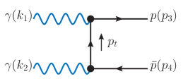
(a)
(b)
(c)
(d)
Figure 1: Diagrams for the production of in collisions.
We consider the - and -channel proton exchange
(diagrams (a) and (b), respectively),
the exchange of meson in the -channel (diagram (c)),
and the hand-bag mechanism (diagram (d)
plus the one with the photon vertices interchanged).
Here stands generically for a meson.
The kinematical variables used in the present paper are
(see Fig. 1)
(5)
(6)
(7)
We shall work in the c.m. frame of the reaction (1);
see Fig. 18 in Appendix A.
For the incoming photons we use the polarization vectors (65)
and the helicity spinors for the proton are as in (40) – (42)
with , .
The helicity spinors for the antiproton
are obtained from (58) and (48), (49),
with , .
There are 16 helicity amplitudes
(8)
Here ,
and ,
are the helicity labels of proton, antiproton and the photons,
respectively. We have also introduced
a convenient shorthand notation for the amplitudes.
Using rotational, parity and charge-conjugation invariance
one finds that only 6 of the 16 helicity amplitudes
are independent which we denote by , …, ;
see (77) and Table 5 of Appendix A.
The unpolarized differential cross section
for the reaction (1) is given by
(9)
where is the invariant mass squared of the system,
denotes the angle of the outgoing nucleon relative to the beam
direction in the c.m. frame, see Fig. 18
in Appendix A,
and and are the c.m. 3-momenta
of the initial photon and final nucleon, respectively; see (64).
II.1 Nonresonant proton exchange contribution
The amplitude for the proton exchange mechanism
[see the diagrams (a) and (b) in Fig. 1]
is written as
(10)
Here we use the free proton propagator for the internal proton lines
and the photon-proton vertex function
as for on-shell protons respectively antiprotons.
This photon-proton vertex function is,
with , given by
(11)
see e.g. (3.26) of Ewerz:2013kda .
In (11) ,
and are the Dirac and Pauli form factors of the proton,
respectively. For real photons we have
and ,
where is the anomalous magnetic moment of the proton.
The amplitude (10) satisfies the gauge-invariance relations (3) and the Bose-symmetry relation (4).
Of course, the virtual protons in the diagrams of Fig. 1 (a) and (b)
are off shell. Their propagators will, in general, not be the ones of free protons
and the photon-proton vertex functions also will have an off-shell dependence.
We take these off-shell dependences into account
via multiplication of the amplitude (10)
by an extra form factor.
We adopt here the scheme used in previous works
Poppe:1986dq ; Szczurek:2002bn ; Klusek-Gawenda:2013rtu ; Lebiedowicz:2014bea
and set
(12)
with the exponential parametrizations
(13)
The parameter should be fitted to the experimental data.
Note that the form factor is normalized to unity for .
Our complete result for the nonresonant proton exchange contribution reads, therefore,
(14)
The multiplication of the “bare” amplitude with a common form factor
guarantees that the gauge-invariance relations (3)
are satisfied for .
Also the Bose-symmetry relation (4)
is satisfied
222The amplitude for
considered in Eqs. (8) - (10) of Ahmadov:2016sdg
does not satisfy the Bose-symmetry relation (4).
Therefore, this amplitude and the corresponding cross section,
(16) and (20) of Ahmadov:2016sdg , cannot correspond to reality.
by (14) since
satisfies (4)
and the form factor is symmetric under the exchange
; see (10) and (12).
II.2 meson contributions
In this section we discuss the contributions from the -channel exchange
of mesons, generically denoted by in diagram (c)
of Fig. 1.
In the following we shall take into account
the and resonances.
That is, in the formulas stands for any of these resonances.
In the final calculations their contributions are summed.
The amplitude for the production through
the -channel exchange of a tensor meson
[the corresponding diagram is shown in Fig. 1 (c)]
is written as
(15)
The vertex is given as
(16)
with two rank-four tensor functions,
(17)
(18)
see (3.39) and (3.18) – (3.22) of Ewerz:2013kda .
In our case we have .
For the meson, the coupling constants
and
are estimated in Secs. 5.3 and 7.2 of Ewerz:2013kda .
In the case of the meson the numerical values of the and parameters
will be obtained here from a fit to the Belle data Kuo:2005nr .
In (16) we have introduced form factors
describing the dependence of the coupling.
These form factors will be particularly important for the diagram
Fig. 1 (c) with exchange
since in production this meson significantly contributes
but only far off shell.
Let us now discuss in detail the vertex.
From the - analysis, presented in Appendix B,
we know that there are two independent couplings
corresponding to and .
In accord with this we choose two coupling Lagrangians, (19) and (20) below,
which correspond to two linearly independent combinations of the two possibilities;
see Appendix B. We set
(19)
(20)
where and are the proton and meson field operators, respectively.
The corresponding vertices, including form factors, are
(21)
(22)
Here () are dimensionless coupling constants
and GeV.
The complete vertex function is given by
(23)
For the propagator we use the simple formula
(24)
where .
is the total decay width of the resonance
and its mass.
For a more detailed analysis we should use a model for the propagator
along the lines considered in Ewerz:2013kda ;
see (3.6) – (3.8) and Appendix A of Ewerz:2013kda .
With the expressions from Appendix A
we get the helicity amplitudes
for the reaction ,
using the notation of (74)
and
as defined in (54), as follows
(25)
(26)
Note the different dependences in (25) and (26)
that are due to the different dimensions of
and .
Using different functional forms for the form factors and
these dependences could be adjusted to experimental data.
In the calculation we assume the same form for and
(27)
A convenient ansatz for such a form factor is the exponential one
(see (4.22) of Lebiedowicz:2016ioh )
(28)
with a parameter of the order 1 – 2 GeV.
Alternatively, we can use
(29)
The form factors (28) and (29)
are normalized to .
For the form factors we assume
(30)
The numerical values of the form factor parameters will be adjusted to the Belle
experimental data.
II.3 Hand-bag approach
The hand-bag contribution to processes
was described in detail in Diehl:2002yh .
The hand-bag amplitude can be written in terms of the hard scattering
kernel for
and a soft matrix element describing the transition.
Their c.m. helicity amplitudes, which we denote by ,
are written in terms of the light-cone helicity amplitudes
(see Eq. (30) in Diehl:2002yh ) as
(31)
The light-cone helicity amplitudes,
including terms suppressed only by ,
read Diehl:2002yh
(32)
The authors of Diehl:2002yh argue that
the amplitudes with identical photon helicities
will be nonzero only at next-to-leading order in ,
in analogy to the photon helicity flip transitions
in large-angle Compton scattering Huang:2001ej .
Note that for zero mass the light-cone helicity amplitudes (32)
are identical with the helicity amplitudes (31),
but not if the mass is finite.
The transition form factors
, and
were determined phenomenologically in Diehl:2002yh .
In our calculation we neglect the term with
and assume
(see formula (45) from Diehl:2002yh ).
In addition we take and as real and positive.
We parametrize (in parameter set A)
with a parameter of dimension GeV2 or
(in parameter set B)
with a parameter of dimension GeV4
which we shall determine from a fit to the Belle data in Sec. IV.3;
see Table 2.
Note that the -dependence of with is different (less steep)
than in Diehl:2002yh , where only the hand-bag contribution
was fitted to rather old experimental data.
In Diehl:2002yh different phase conventions compared to ours are used.
Taking this into account we find
The hand-bag helicity amplitudes (33)
must be added coherently within our approach (see previous subsections).
At small momentum transfer or
the hand-bag and proton-exchange mechanisms compete
and it would be a double counting to include both of them simultaneously.
We emphasize, however, that in regions of small or
the hand-bag approach has to be taken with a grain of salt.
To avoid in addition double counting
(we include explicitly the proton-exchange mechanism) we suggest
to multiply the hand-bag amplitudes by a purely phenomenological factor:
(34)
with an extra free parameter .
Its role is to cut off the region of small and
where the hand-bag approach does not apply.
As a consequence it also reduces the hand-bag contribution
to the cross section at low in the whole angular range.
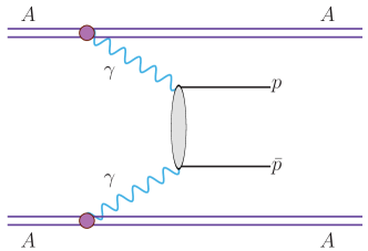
III Nuclear reaction
Now we will present theoretical formulas for the nuclear reaction
(35)
Figure 2: Diagram representing proton-antiproton production in ultrarelativistic
ultraperipheral collisions (UPC) of heavy ions.
We focus on the processes for ultraperipheral collisions (UPC) of heavy ions,
see the diagram shown in Fig. 2.
The nuclear cross section is calculated in the equivalent photon approximation (EPA)
in the impact parameter space.
This approach allows to take into account the transverse distance between the colliding nuclei.
The total (phase space integrated) cross section
is expressed through the five-fold integral
(36)
Above, is the impact parameter, i.e., the distance between colliding nuclei
in the plane perpendicular to their direction of motion.
is the invariant
mass of the system and , ,
is the energy of the photon which is emitted from the first or second nucleus, respectively.
is the rapidity of the system.
The quantities
,
are given in terms of , which are the components of
the and vectors
which mark a point (distance from first and second nucleus)
where photons collide and particles are produced.
The diagram illustrating these quantities in the impact parameter
space can be found in KlusekGawenda:2010kx .
In Ref. KlusekGawenda:2010kx the dependence of the photon flux
on the charge form factors of the colliding nuclei
was shown explicitly.
In our calculations we use the so-called realistic form factor
which is the Fourier transform of the charge distribution in the nucleus.
A more detailed discussion of this issue is given in KlusekGawenda:2010kx .
The presence of the absorption factor in (36)
assures that we consider only peripheral collisions,
when the nuclei do not undergo nuclear breakup.
In the first approximation this geometrical factor
can be expressed as
(37)
where the sum of the radii of the two nuclei occurs.
In our present study we calculate also distributions in kinematical variables
of each of the produced particles (for details
how it is handled see Klusek-Gawenda:2016euz ).
Then one can impose easily experimental cuts on (pseudo)rapidities and transverse momenta.
IV Results for the reaction
First we will show some features of the
proton-exchange mechanism and the -channel tensor meson exchanges.
We will show the dependence of the cross section on the photon-photon energy
and the angular distributions of individual helicity components.
Then we will confront the model results with the experimental data
and adjust the model parameters.
IV.1 Proton exchange mechanism
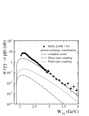
In Fig. 3 we show that the proton exchange mechanism alone
cannot describe the energy-dependence of the cross sections measured by Belle Kuo:2005nr .
We show results for the Dirac- or Pauli-type couplings separately
and when both couplings in the vertices are taken into account.
We can see that the complete result indicates a large interference effect
of Dirac and Pauli terms in the amplitudes.
Clearly, the proton exchange contribution is not sufficient to describe the Belle data.
Figure 3: The cross section as
a function of photon-photon energy .
We present the results for the nonresonant contribution (see Sec. II.1)
for GeV in (II.1).
The solid line represents the complete result with both Dirac- and Pauli-type couplings
included in the amplitude.
Other combinations of electromagnetic couplings in the vertices
are also shown: only Dirac couplings, and only Pauli couplings
at the two vertices in Figs. 1 (a) and (b).
The Belle experimental data from Kuo:2005nr are shown for comparison.
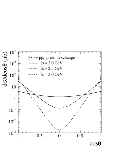
In Fig. 4 we show
the unpolarized differential cross section
for three different c.m. energies.
As one gets closer to , the threshold energy,
the angular distributions become flatter and flatter.
Figure 4: The angular distributions for = 2.0, 2.5 and 3.0 GeV
for the nonresonant proton-exchange mechanism.
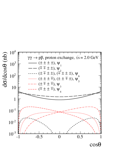
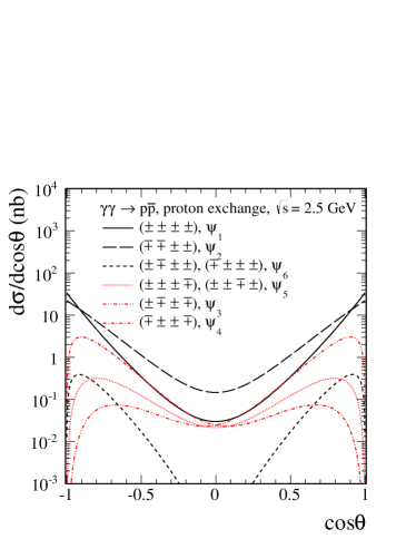
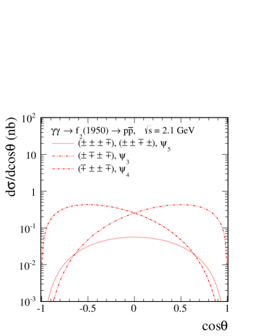
In Fig. 5 we present
the helicity dependence of the differential cross section.
We label the results for different helicity terms as
for
as defined in (74).
One can see the dominance of the
and contributions
over the ones (see the red lines).
In terms of the () from (77)
and Table 5 of Appendix A
we find dominance of the amplitudes and .
Furthermore we see that the contributions of the amplitudes
, , and
are suppressed in the forward and backward directions, .
This is clear from angular momentum conservation.
For , , and ,
the state of the two photons has .
This cannot be reached by proton-antiproton produced in the
forward or backward direction where we only get or .
For the two-photon state has
and the two-baryon state in forward and backward direction has and -1,
respectively. We have again a mismatch.
The contributions of four helicity states
, , ,
vanish when only the Dirac-type coupling in the vertices is included.
That is, the amplitude vanishes in this case.
Figure 5: The helicity components of as a function of
for the proton exchange mechanism
for (the left panel) and 2.5 GeV (the right panel).
Contributions of different helicities
of the photons and baryons are shown.
IV.2 meson contributions
The Belle experimental angular distributions Kuo:2005nr ,
at least at low energies,
cannot be described solely with the proton-exchange mechanism
discussed in Sec. II.1.
It seems that a mechanism is missing.
A resonant -channel contribution is a reasonable option
for a second mechanism (see also Klusek-Gawenda:2013rtu
for the reactions).
In Table 1 we have listed resonances that
decay into and and which,
therefore, may contribute to the reaction (1).
In principle, also subthreshold resonances,
such as , may play some, even an important, role.
It is worth to mention that our knowledge
about the resonance comes from the BES Ablikim:2006pt
and the CLEO Alexander:2010vd analyses
for radiative decays.
In Alexander:2010vd the authors include also the contribution
in order to describe
the and invariant mass distributions.
For a stringent upper limit
for the threshold resonance
at 90% confidence level was found Alexander:2010vd .
Table 1: A list of resonances that may contribute to the reaction.
Here we listed also the subthreshold resonance.
The meson masses, their total widths and branching fractions
are taken from PDG Olive:2016xmw .
Meson
(MeV)
(MeV)
seen
seen
In our paper we consider only the meson exchanges in the -channel.
In general also the mesons (e.g. , )
may contribute to the reaction (1).
The charmonium states have rather small total widths (see Table 1)
thus they will appear in the invariant mass distribution as rather narrow peaks;
see Lebiedowicz:2017cuq for the reaction.
Even interference effects with other mechanisms may be important in this context.
This goes, however, beyond the scope of the present paper and will be studied elsewhere.
Now we will discuss the helicity structure of
from the contribution of the -channel
(below-threshold or above-threshold) resonances in our
Lagrangian approach; see Sec. II.2.
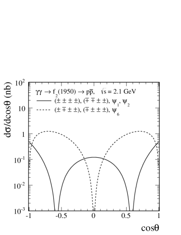
In Fig. 6 we show the contributions of
different helicities for the two couplings in (16),
(left panel)
and (right panel).
There are five independent helicity contributions
since here the contributions of the amplitudes and
turn out to be the same; see (25),
(77) and Table 5 of Appendix A.
Only the distributions that are proportional to ,
see (25) and (26),
(this corresponds to the solid line in the left panel)
are favored by the Belle experimental data;
see Figs. 8 and 9 below.
Here the cutoff parameter of form factors () and
the products of coupling constants ( and
)
are fixed arbitrarily.
Figure 6: The helicity components of the differential cross sections
for the reaction
for GeV.
Here, the coupling constants are fixed arbitrarily, for :
GeV-3 (the left panel) and
GeV-1 (the right panel).
The calculations have been done for GeV
in (29).
IV.3 Comparison with the Belle data
Here we wish to demonstrate that it is possible
to describe the Belle data taking into account
the - and -channel proton exchanges,
the -channel tensor meson exchanges,
and the hand-bag mechanism
discussed in Sec. II.
In the following we shall take in our calculation
a coherent sum of all the above amplitudes.
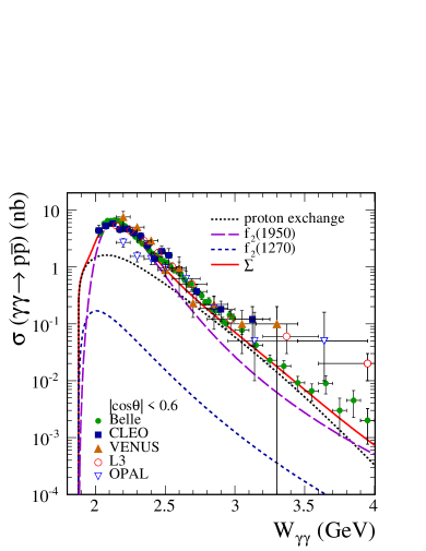
In Fig. 7 we show the energy dependence of the cross section
for the reaction.
In the panel (a) we present results for the proton exchange and
the and -channel exchanges
together with the experimental data of the CLEO Artuso:1993xk ,
VENUS Hamasaki:1997cy ,
OPAL Abbiendi:2002bxa ,
L3 Achard:2003jc ,
and Belle Kuo:2005nr experiments.
An agreement between the Belle experimental data Kuo:2005nr
and the earlier measurements Artuso:1993xk ; Hamasaki:1997cy ; Achard:2003jc
with the exception of the OPAL experiment Abbiendi:2002bxa
in the low mass region GeV can be observed
(within the quoted uncertainties); see also Fig. 11 below.
For the contribution the coupling constants
and are relatively well known and
taken from Ewerz:2013kda .
We take into account only one coupling
()
and neglect the term with .
For the contribution we take
only the term with GeV-3.
In the vertices for the meson exchange contributions we assume
the same type of the form factors (29)
and GeV;
see Eqs. (27) and (30).
We take GeV for the proton-exchange contribution; see (II.1).
One can observe the dominance of the resonance term at low energies.
We slightly underestimate the Belle data from to GeV.
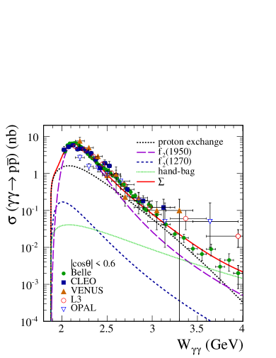
The panels (b) and (c) show results including also the hand-bag contribution.
The hand-bag contribution is important at GeV.
To illustrate uncertainties of our model we take
in the calculation two sets of parameters.
For the convenience of the reader we collect in Table 2
the parameters of our model and their numerical values
used here and in the following.
Table 2: Model parameters and their numerical values used.
The second column indicates the equation numbers where
the parameter is defined.
Figure 7: Energy dependence of the total cross section for
for .
The experimental data are from the CLEO Artuso:1993xk ,
VENUS Hamasaki:1997cy ,
OPAL Abbiendi:2002bxa ,
L3 Achard:2003jc ,
and Belle Kuo:2005nr experiments.
In the panel (a) we show the results
for the tensor meson exchanges and the proton-exchange contributions,
and their coherent sum (see the red solid line).
In the panels (b) and (c) we show the results including, in addition, the hand-bag contribution.
In the panels (a) and (b) we used the parameter set A
while in the panel (c) we used the parameter set B; see Table 2.
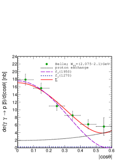
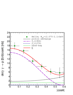
In Figs. 8 and 9,
we show our fits to the Belle angular distributions
333The cross section , , was calculated
for the Belle angular range of ,
but plotted for after multiplication by a factor 2..
Here we use the same parametrization as in Fig. 7 (a)
(see set A of Table 2).
In Fig. 8 we present results
for the , and proton-exchange contributions separately,
as well as their coherent sum.
At large angles, ,
the inclusion of the contribution
lowers the cross section compared to the case when
only the and proton-exchange are taken into account.
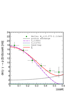
In Fig. 9 we show results including the hand-bag contribution.
The parameter obtained from the fit is GeV2.
In Fig. 10
we use, as in Fig. 7 (c), the parameter set B of Table 2.
The parameter obtained from the fit is GeV4.
In Ref. Diehl:2002yh was estimated
to be in the range GeV4
which is the same order of magnitude as we find.
Experimentally the angular distributions were
averaged over rather large intervals of (sub)process energies.
For a better comparison with the experimental data
we use the formula, with ,
(38)
instead of .
(a)
(b)
(c)
(d)
(e)
(f)
(g)
(h)
(i)
(j)
(k)
Figure 8: Differential cross sections for the reaction
as a function of for different ranges.
For the Belle data Kuo:2005nr
both statistical and systematic uncertainties are included.
Calculations were done with
GeV
in (29),
and GeV in (II.1).
The hand-bag model contribution is not included here.
Here we used the parameter set A from Table 2.
(a)
(b)
(c)
(d)
(e)
(f)
(g)
(h)
(i)
(j)
(k)
Figure 9: The same as in Fig. 8 but here
the hand-bag contribution is included.
The green dotted line shows the contribution of the hand-bag mechanism.
Here we used the parameter set A from Table 2.
(a)
(b)
(c)
(d)
(e)
(f)
(g)
(h)
(i)
(j)
(k)
Figure 10: The same as in Fig. 9
but here we used the parameter set B from Table 2.
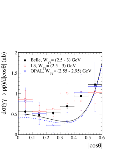
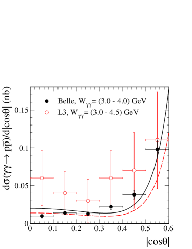
In Fig. 11 we compare the Belle data Kuo:2005nr
and the earlier OPAL and L3 data Abbiendi:2002bxa ; Achard:2003jc
with our model results.
Due to the large error bars of the OPAL and L3 data
only the comparison of the model results with the Belle data
gives significant information.
Figure 11: Differential cross sections for the reaction
as a function of
for different ranges.
We compare our total model results (including the hand-bag contribution)
with the Belle data Kuo:2005nr ,
the L3 data Achard:2003jc ,
and the OPAL data Abbiendi:2002bxa ;
see the black solid line, the red long-dashed line,
and the blue short-dashed line, respectively.
Here we used the parameter set A from Table 2.
Heaving shown that the results of our approach,
including three mechanisms, describe the Belle experimental data reasonably well
we shall present our predictions for the nuclear reaction (35)
in the next section.
V Predictions for the nuclear ultraperipheral collisions
Having described the Belle angular distributions
we go to the predictions for the nuclear collisions.
In this section we show the integrated cross sections
and several differential distributions
for the nuclear process (35)
calculated as described in Sec. III
including three mechanisms
discussed in Secs. II and IV.
In the calculations below we used the parameter set A
from Table 2.
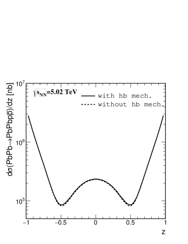
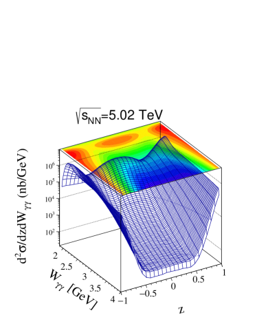
Figure 12: The distribution in , integrating over
GeV,
for the reaction
at the collision energy TeV.
Figure 13: Distribution in ()
for the reaction (35)
at the LHC energy TeV.
In Fig. 12 we present
the angular distribution
( in the c.m. system)
at the collision energy TeV.
Here we show the nuclear results when the hand-bag mechanism
is included (solid line) and excluded (dotted line).
One can conclude that the hand-bag contribution does not play an important role
in the angular distribution.
We wish to emphasize that the enhancements at are the consequence
of our model presented in Sec. II.
One can better visualize this behavior with the help of
the two dimensional distribution .
From Fig. 13 we clearly see that
the result for the nuclear reaction corresponds to
that for elementary reaction
discussed in the previous section.
The contribution dominates at smaller and
at and .
This coincides with the result which was presented
in Fig. 6 (left panel, solid line).
In contrast to the resonant contribution,
the proton-exchange one is concentrated mostly at larger invariant masses
and around .
(a)
(b) (c)
(d)
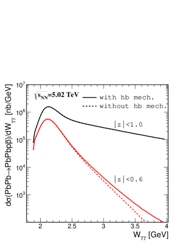
Figure 14: The differential nuclear cross sections
for the reaction (35)
at TeV.
Results for the full range of (the black lines)
and for (the red lines) are presented.
In panels (b) - (d) we integrate for GeV.
No other cuts have been imposed here.
In Fig. 14 we present
the nuclear differential cross sections for two ranges of :
the red lines are for , as in the Belle measurement,
the black lines are for (full range).
Panel (a) shows the distribution in proton-antiproton invariant mass
().
The distribution for the full -range extends
to much larger invariant masses
while for the Belle -range it falls steeply down.
Similar as for the elementary cross section (Fig. 7),
the hand-bag mechanism contributes significantly at GeV.
Simultaneously, the difference between the results with (solid lines)
and without (dotted lines) hand-bag contribution appears
more pronounced for the case
when the angular phase space is narrowed.
In the present calculations we integrate
for GeV.
The transverse momentum distributions of protons and antiprotons
shown in panel (b) are identical. Therefore we label them by .
For large the distributions fall steeply.
The limitation on the phase space ()
has a significant impact for smaller values of
and has no influence for GeV.
In the panel (c) we show distributions
in rapidity of the proton or antiproton (which are identical).
Here we see only a difference in the normalization,
and not in the shape for the two different ranges of .
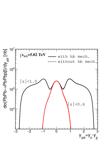
Finally, in the panel (d) we show the distribution in rapidity
distance between proton and antiproton .
The larger the range of phase space
the broader is the distribution in .
There are three maxima when no extra cuts are imposed.
The broad peak at corresponds to the region .
It seems that observation of the broader distribution,
in particular identification of the outer maxima, could be a good test of our model.
As we see from Fig. 12 the cross section
decreases quickly with
for , but stays large for .
Thus, extending the integration to GeV
should not change the distributions of Fig. 14 (b) - (d)
for but could have a sizeable influence on
those for .
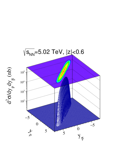
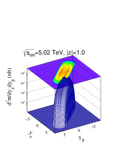
Figure 15: The two-dimensional distributions in proton and antiproton rapidities
for the reaction (35) at TeV
for two different -ranges of outgoing nucleons.
The results include the hand-bag contribution.
The results are integrated for GeV.
In Fig. 15 we show
the two-dimensional distributions in ()
again for two ranges of (left panel relates to the Belle angle limitation
and right panel is for full phase space).
The cross section is concentrated along the diagonal .
The ALICE Collaboration can measure in - collisions
for ;
see Kryshen:2017jfz where the decay was observed.
444We thank E. L. Kryshen for some information on the recent ALICE measurement.
We predict 46 events for and GeV
for our contribution,
including three mechanisms,
for ALICE integrated luminosity b-1Kryshen:2017jfz .
On the other hand the coherent photoproduction Klusek-Gawenda:2015hja
in the channel gives 583 events
assuming approximately isotropic decay of .
This strongly suggests dominance of the coherent photoproduction mechanism of
over the contribution.
With such a transverse momentum cut
as for the ALICE preliminary result
a lot of the contribution
is lost (with respect to the full phase space)
but considerably less of coherent contribution,
where the maximum of the emission occurs
at GeV
(sharp Jacobian peak associated with the fact that
transverse momentum of the coherent is very small).
Generally, the range covered by the ATLAS and CMS detectors
for pairs in UPC is somewhat larger, .
The LHCb Collaboration can measure production in nuclear collisions
for and GeV.
555We thank R. McNulty and T. Shears for some information on the recent LHCb measurement.
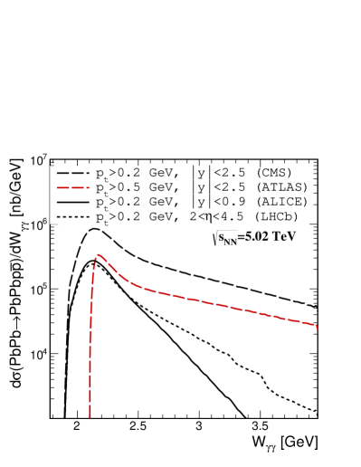
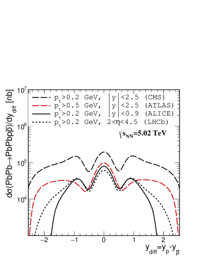
Figure 16: The differential nuclear cross sections as a function of invariant mass
(the left panel) and (the right panel)
for the reaction (35).
The results for different experimental cuts are presented.
In Fig. 16 we present distributions in
(the left panel) and
(the right panel)
imposing cuts on rapidities and transverse momenta of outgoing baryons.
From the left panel, we can observe that
the dependence on invariant mass of the pair
is sensitive to the (pseudo)rapidity cut imposed.
Note that due to the cut on GeV
the distribution begins with a larger value of 2.1 GeV
(compare also with Fig. 14 (a)).
The distribution in the difference of proton and antiproton rapidities is interesting.
Again (comparing with Fig. 14 (d), )
the -distributions show three maxima.
The experimental cuts imposed on do not remove the external
maxima predicted by our model.
Such characteristic features can be checked by future experiments.
For completeness, we give the cross sections
for the
reaction for the contribution
for various experimental cuts on proton and antiproton (pseudo)rapidities
and transverse momenta at TeV.
We find the cross section of 100 b taking into account the ALICE cuts
(, GeV),
160 b for the ATLAS cuts (, GeV),
500 b for the CMS cuts (, GeV),
and 104 b for the LHCb cuts (, GeV).
VI Conclusions
We have discussed in detail the production of proton-antiproton pairs
in photon-photon collisions. Previous theoretical papers on the subject
tried to pick up only one simple mechanism out of many in principle possible ones.
In our work we have tried to incorporate the known mechanisms,
such as proton exchange, -channel resonance exchange and the hand-bag contribution.
In our calculation of the nonresonant proton exchange
we have included both Dirac- and Pauli-type couplings of the photon to the nucleon
and form factors for the exchanged off-shell protons.
We have found that the Pauli-type coupling is very important,
enhances the cross section considerably, and cannot therefore be neglected.
We have shown that the Belle data Kuo:2005nr for low photon-photon energies
can be nicely described by including in addition to the proton exchange
the -channel exchange of the resonance,
which was observed to decay into the and channels Olive:2016xmw .
We include in the calculation also the -channel meson exchange contribution.
These two tensor mesons were also needed to describe the Belle data
for the and
processes Uehara:2009cka ; Klusek-Gawenda:2013rtu .
Our simple model has a few parameters; see Table 2.
Adjusting the parameters of the vertex form factors for the proton exchange,
of the tensor meson -channel exchanges,
and of the form factor (34) in the hand-bag contribution
we have managed to describe both total cross section
and differential angular distributions of the Belle Collaboration
with significantly better agreement with the data than in all previous trials.
Having described the Belle data we have used the
cross section to calculate
the integrated cross section and differential distributions
for production of pairs in
ultraperipheral, ultrarelativistic, collisions (UPC) of heavy ions
at TeV.
We have presented distributions in rapidity
and transverse momentum of protons and antiprotons,
invariant mass of the system as well as
in the difference of rapidities for protons and antiprotons.
We have presented results for the full angular range of
as well as for the Belle range .
The integrated cross section for the full phase space
is by a factor 5 larger than the one corresponding to the Belle angular coverage.
The larger the range of phase space
the broader is the distribution in ,
the rapidity difference between proton and antiproton.
We have also made predictions for - collisions at
TeV and experimental cuts for
the ALICE, ATLAS, CMS, and LHCb experiments.
Corresponding total cross sections and differential distributions have been presented.
The UPC of heavy ions may provide
new information compared to the presently available data from
collisions, in particular, if the structures
of the distributions shown in Figs. 14
and 16 can be observed.
Acknowledgements.
The authors are grateful to Markus Diehl for correspondence and
comments and to Carlo Ewerz for discussions.
This research was partially supported by
the Polish National Science Centre Grant No. DEC-2014/15/B/ST2/02528 (OPUS),
the MNiSW Grant No. IP2014 025173 (Iuventus Plus),
and by the Center for Innovation and Transfer of Natural Sciences
and Engineering Knowledge in Rzeszów.
Appendix A Helicity states for protons and antiprotons and helicity amplitudes
The general theory of helicity amplitudes
for collisions of particles with spin was developed in Jacob:1959at .
To make our article selfcontained and to fix the phases
of our states we discuss in the following the construction of helicity states
for protons and antiprotons as we found convenient for our purposes.
These states are then used to determine
the independent helicity amplitudes
for the reaction (1).
We consider protons and antiprotons in a fixed reference frame;
see Fig. 17.
Let be the 3-momentum of the proton and
(39)
We use throughout our paper a boldface notation for 3-vectors, , etc.
Figure 17: Coordinate system and momentum vector .
For ()
we define the spinors of definite helicity of type as
(40)
where
(41)
This gives
(42)
(43)
Let us denote the usual spinors with spin in direction as
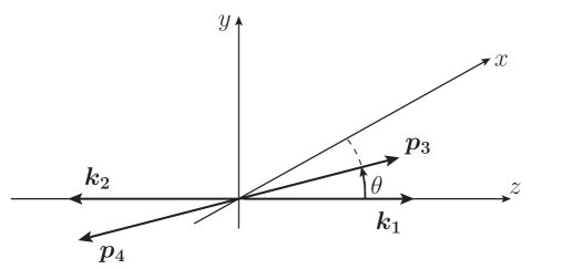
Now we come to the reaction (1).
We consider (1) in the c.m. system
with the - plane giving the reaction plane; see Fig. 18.
Figure 18: The reaction in the c.m. system.
The usual kinematic variables are given by (5).
Let , , be the Cartesian unit vectors
in the reference system of Fig. 18.
Then
and the momenta of the particles are
(64)
As polarization vectors for the incoming photons of definite helicity
we choose
(65)
The corresponding photon creation operators are
(66)
For the proton we choose the helicity basis , for the antiproton
the basis . From (46) and (61)
we have for the corresponding creation operators
(67)
(68)
Note that in calculating from (45)
we have to make the replacements
, .
Calculating from (51)
we have to make the replacements
, .
The symmetries of the reaction (1) are the following.
The parity () transformation followed by a rotation by
around the positive -axis:
(69)
The charge-conjugation () transformation followed by a rotation
by around the positive -axis:
(70)
From the transformation laws of the standard creation operators (see e.g. Nachtmann:1990ta )
and from the relations (see (45), (51))
(71)
(72)
we get the transformation laws for the helicity creation operators shown in Table 3.
Table 3: Transformation properties of creation operators for protons,
antiprotons, and photons under the transformations (69) and (70).
We define now the helicity states for the reaction (1)
using (66), (67) and (68) as
(73)
The transformation laws of these states are shown in Table 4.
Table 4: Transformation laws of the states
(A) under the transformations (69) and (70).
Finally we come to the helicity amplitudes for the reaction (1)
(74)
where we use the convenient shorthand notation of (8).
There are 16 helicity amplitudes.
The symmetry (69) gives the relation,
using Table 4,
The relations (75) and (76)
are written explicitly for the helicity amplitudes in Table 5.
From this we find that there are only 6 independent helicity amplitudes
for (1) which we choose as follows:
(77)
Table 5: Helicity amplitudes for (1)
and their symmetry relations.
With this we have obtained a complete overview of the general constraints
of the helicity amplitudes of
following from rotational, parity, and charge-conjugation invariance
of strong and electromagnetic interactions.
Finally we note that the same analysis applies to any reaction
(78)
where stands for a spin baryon.
We only have to replace in all our formulas by .
Interesting examples may be , .
666The baryon has a magnetic moment
Olive:2016xmw .
Thus, the reaction
can proceed through the analogue of the diagrams
of Fig. 1 (a) and (b).
The polarization of these baryons can be
obtained from their decay distributions.
Appendix B The coupling scheme and helicity amplitudes for the reaction
In this Appendix we discuss the relation of couplings
to the helicity amplitudes for the reaction .
Here stands for the orbital angular momentum and
for the total spin of the system.
Let us see in how many ways one can construct a state
with .
The partial-wave analysis (which is perfectly relativistic)
says that we can combine the spins
of and to give the total spin .
Now we must combine this with the orbital angular momentum to
the total angular momentum .
This gives the four possibilities listed in Table 6.
In general we have the parity of state
( and have opposite intrinsic parity)
and charge-conjugation .
There are, thus, two possible couplings for :
and .
2
0
1
1
2
1
3
1
Table 6: The and values leading to states with .
We shall now analyze the content of the couplings
(19) and (20).
Let , be the usual Dirac spinors with
spin in direction for ;
see (44) and (56).
For these we find in the c.m. system of reaction (1)
the matrix elements of the vertex functions
()
(see (21), (22))
with
the spin 2 projector (the term in square brackets in (24)) as follows.
For we get
(79)
(80)
Here and in the following we set ;
see (44) and (56). For we get
(81)
(82)
The - amplitudes are as follows.
For , we have
(83)
The traceless symmetric () tensor is
(84)
This gives, for instance, with as defined in Fig. 18
and the Legendre polynomial
(85)
The , the amplitude is
(86)
From (80), (82), (83) and (86)
we get the - decomposition of our couplings and 2 as follows:
(87)
(88)
Note that – for and
not depending on –
clearly has only
and clearly has only ;
see (83) and (86), respectively.
But now we can go to the helicity amplitudes.
All we have to do is to replace the two-component spinors
as follows
(89)
Note that these spinors depend on .
We get
(90)
Inserting these expressions in (80) and (82)
we see that the dependence, that is,
the dependence of the amplitudes
will in general be changed.
Take, for instance, (82)
which is a combination of plus ;
see (83) and (86).
With the replacements (89) we get from (90)
(91)
From plus we go, effectively, to .
The replacements (89) lead from (80) and (82),
using the expression for the diagram for
[see Fig. 1 (c)],
to the helicity amplitudes (25) and (26).
Appendix C Phase conventions
For the hand-bag contribution, Sec. II.3,
we must take into account different phase conventions
used in Diehl:2002yh relative to ours,
as explained in Appendix A.
In Diehl:2002yh the orientation of the particle
momenta corresponds to a rotation by
relative to the momenta in Fig. 18.
Considering this we find that their spinors for
proton and antiproton correspond to our
and , respectively.
The phase conventions for the photons are not stated explicitly in Diehl:2002yh .
From a comparison
777We thank M. Diehl for correspondence on this point.
of the calculations (22) and (23) of Diehl:2002yh
with the corresponding ones with our conventions we conclude that
the states of Diehl:2002yh
have an extra minus sign compared to ours.
Taking everything together we obtain (33) for the amplitudes.
(2)
H. Hamasaki et al., (VENUS Collaboration), Measurement of the
proton-antiproton pair production from two-photon collisions at TRISTAN,Phys. Lett. B407 (1997) 185–192.
(6)
G. R. Farrar, E. Maina, and F. Neri, QCD Predictions for
Annihilation to Baryons,Nucl. Phys. B259 (1985) 702–720.
[Erratum: Nucl. Phys.B263,746(1986)].
(7)
G. R. Farrar, H. Zhang, A. A. Ogloblin, and I. R. Zhitnitsky, Baryon Wave
Functions and Cross-sections for Photon Annihilation to Baryon Pairs,Nucl. Phys. B311 (1989) 585–612.
(8)
V. L. Chernyak and I. R. Zhitnitsky, Nucleon wave function and nucleon
form factors in QCD,Nucl. Phys. B246 (1984) 52–74.
(17)
P. Lebiedowicz, O. Nachtmann, and A. Szczurek, and
Drell-Söding contributions to central exclusive production of pairs in proton-proton collisions at high energies,Phys. Rev. D91 (2015) 074023,
arXiv:1412.3677 [hep-ph].
(18)
P. Lebiedowicz, O. Nachtmann, and A. Szczurek, Central exclusive
diffractive production of the continuum, scalar, and tensor
resonances in and scattering within the tensor Pomeron
approach,Phys. Rev.
D93 (2016) 054015,
arXiv:1601.04537 [hep-ph].
(20)
M. Kłusek-Gawenda and A. Szczurek, Exclusive muon-pair productions in
ultrarelativistic heavy-ion collisions: Realistic nucleus charge form factor
and differential distributions,Phys. Rev. C82 (2010) 014904,
arXiv:1004.5521 [nucl-th].
 (b)
(b)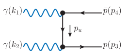 (c)
(c)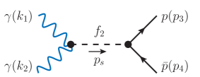 (d)
(d)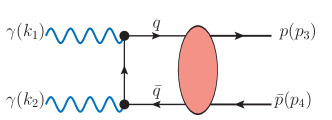
 (c)
(c)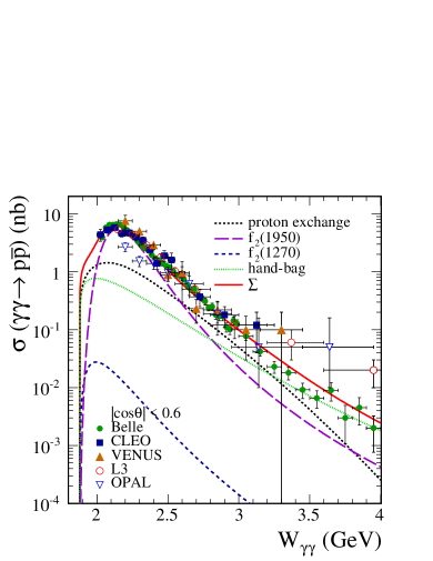
 (b)
(b)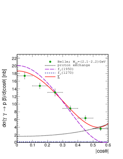 (c)
(c)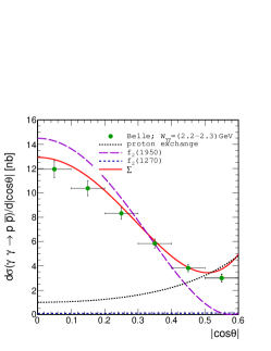 (d)
(d) (e)
(e)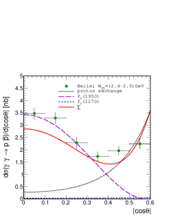 (f)
(f)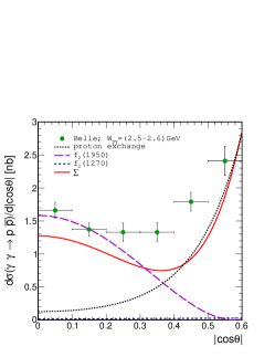 (g)
(g)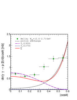 (h)
(h)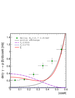 (i)
(i)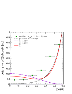 (j)
(j)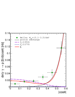 (k)
(k)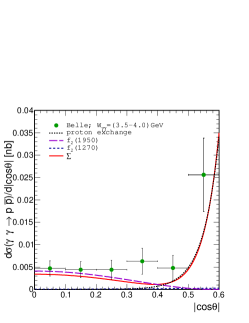
 (b)
(b)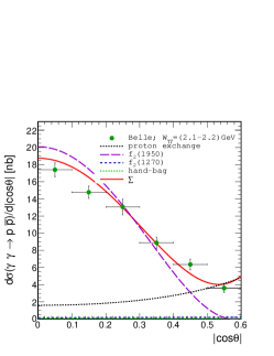 (c)
(c)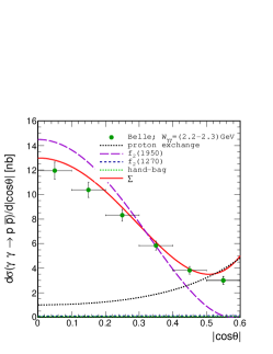 (d)
(d)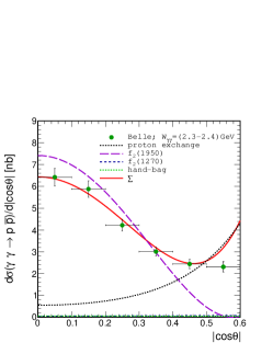 (e)
(e)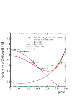 (f)
(f)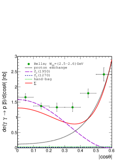 (g)
(g)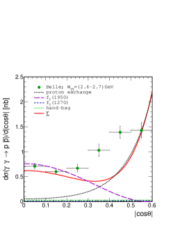 (h)
(h) (i)
(i)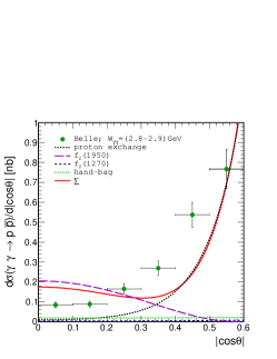 (j)
(j) (k)
(k)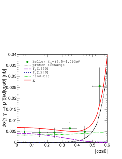
 (b)
(b)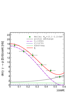 (c)
(c)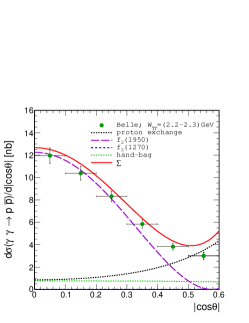 (d)
(d)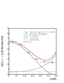 (e)
(e)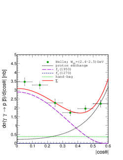 (f)
(f)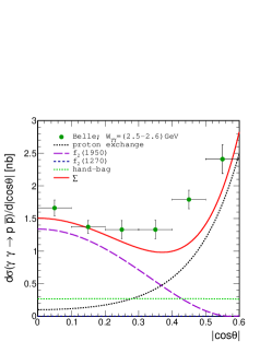 (g)
(g)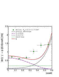 (h)
(h)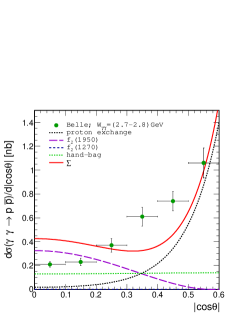 (i)
(i) (j)
(j)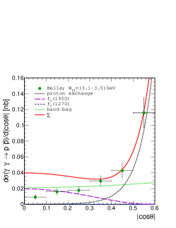 (k)
(k)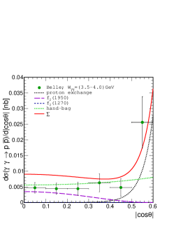

 (b)
(b)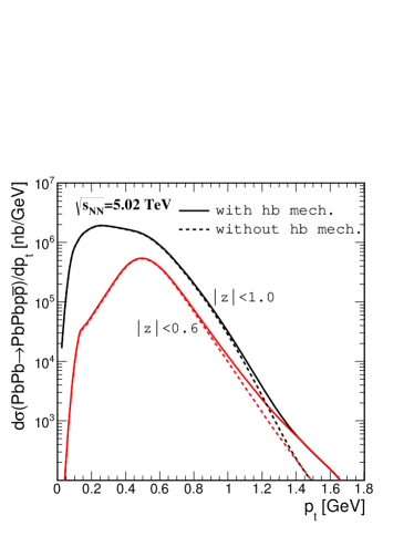
 (d)
(d)